A Comprehensive Numerical Overview of the Performance of Godunov Solutions Using Roe and Rusanov Schemes Applied to Dam-Break Flow

Abstract

As open channel simulations are of great economic and human significance, many numerical approaches have been developed, with the Godunov schemes showing particular promise. To evaluate, confirm, and extend the simulation results of others, a variety of first- and second-order FVMs are available, with Rusanov and Roe schemes being used here to simulate the demanding case of 1D and 2D flows following a dam break. The virtual boundary cells approach is shown to achieve a monotonic solution for both interior and boundary cells, and while flux computation is employed at boundary cells, a refinement is only rarely used in existing models. A number of variations are explored, including the TVD MUSCL-Hancock (monotone upwind scheme for conservation laws) numerical scheme with several slope limiters in a quest to avoid spurious oscillations. The sensitivity of the results to both channel length and the ratio of downstream to initial upstream water depth is explored using 1D and 2D models. The Roe scheme with a Van Leer limiter as a slope limiter is shown to be both fast and slightly more accurate than other slope limiters for this problem, but the Rusanov scheme with different slope limiters works well for 1D simulations. Significantly, the selection of an appropriate slope limiter is shown to be best based on the ratio of the downstream to upstream water depth. However, this study focuses on the special case where the ratio of the initial depth downstream to upstream of the dam is equal to or less than 0.5, and these outcomes are compared to theoretical results. The 2D dam-break problem is used to further explore first- and second-order methods using different slope limiters, and the results show that the Superbee limiter can be problematic due to an observed large dispersion in depth contours. However, the most promising approaches from previous studies are confirmed to deserve the high regard given to them by many researchers.

1. Introduction and Background

Open channel calculations have huge significance in many contexts, from flood studies to power system applications to dam-break problems. The dam-break issue has gained global recognition due to the adverse and often severe effects that flooding can have environmentally and economically, or even to human life. Intense rain, the role of sea-level rise, inadequately controlled urban development, and the possible severity of dam-break events have all increased associated flooding concerns [1]. As tsunamis move along the coast, for example, their wave height often increases, along with their consequences [2,3]. The sudden release of water from a dam break can produce untold human misery and environmental damage [4], sometimes resulting in thousands of lost lives and billions of dollars in damages [5,6,7,8]. For example, the 1889 failure of the South Fork Dam near Johnstown, Pennsylvania (US) occurred after heavy rain, and over 2000 lives were lost [9]. In 2005, a dam collapsed in Brazil and led to a mammoth mud slide that killed 19 people and contaminated a 668 km stretch of river.

Given this importance, many open channel models have been developed with an on-going quest for reliability, accuracy, and stability. Even with inevitable model uncertainty in terms of initial and boundary values and the initiating event, such simulations are often a mandated requirement. Early on, the dam-break problem was studied analytically using a lagrangian description [10]. Unfortunately, early modelling results were approximate and ignored key parameters. Enhanced methods employed the shallow-water form of the Saint-Venant equations [11], an approach that had already been found useful for river forecasting, canal operations, sewer modeling, irrigation, and dam-break simulations [12,13,14,15].

Several numerical models based on shallow-water equations have modeled free surface flow to predict hydraulic failures. A key goal has been to establish a numerical model capable of avoiding spurious results while achieving accurate, stable, and efficient predictions. The approaches included using the finite element method (FEM), an approach that had been used successfully in structural applications. For example, Yang [13] computed one-dimensional unsteady free surface flows resulting from a dam break, specifically by using various characteristics-based high-resolution nonoscillatory shock-capturing finite difference and Petrov-Galerkin finite element methods. From comparisons between the computed results and analytic solutions, researchers demonstrated that accurate predictions of high-speed open channel flows are obtainable. Previous computational solutions to the shallow-water equations have included the finite difference method (FDM) by Hirsch [16], the method of characteristic (MOC) for the kinematic wave equation [17], and the finite volume method (FVM) [18]. Even aside from the need to evaluate the potential consequences of a dam failure, the sudden release of water and the consequent evaluation of flow depth is a crucial numerical test for the evaluation of open channel flow models.

Finite volume schemes have been shown to better resolve the shallow-water equations particularly when they are associated with Godunov-type schemes. Thus, the FVM Godunov-type schemes have proved excellent for solving hyperbolic equations and have been shown to have improved computation of the momentum and mass fluxes [19,20,21]. For example, Hirsch [19] introduced the FVM Godunov-type scheme for shallow-water equations and used a Riemann solver for the fluxes at cell interfaces along with the monotone upwind scheme conservation law (MUSCL) method to achieve second-order spatial accuracy. Subsequently, Vila [22] used a simplified Godunov scheme [23] and achieved second-order accuracy by considering generalized Riemann problems. A physical model of the partial dam break has been developed by Fennema [24]. These authors compared their results with the explicit methods of McCormack and Gabutti. Similarly, a semi-implicit MacCormack scheme allowed adaptation to morphological variation on an alluvial erodible bed [25]. Alcrudo [26] proposed the Riemann problem associated with Roe-type approximation to evaluate inter-flux cell transfers in the 2D dam-break simulations. Sanders [27] used the same approach to solve one-dimensional (1D) shallow-water equations for non-rectangular and non-prismatic channels. The multi-slope concept was recently introduced to solve the problem of MUSCL reconstruction of triangular and tetrahedral unstructured meshes in cell-centered finite volume environments. Unlike the single-slope method, which uses a unique bounded gradient, special scalar slopes are used to compute the interpolation on each side of a given element [28].

Moreover, the high-resolution FVM-Godunov type scheme associated with various limiters is used by Sanders and Bradford [18,20] to analyze the wave propagation near the coastal zone and in the 1D dam-break problem. The total variation diminishing (TVD) schemes are widely applied to the physical problem of moving shocks due to their reduced spurious oscillations [29,30]. In the case of wave propagation near the coastal zone, Gao [31] numerically investigated transient harbor oscillations induced by various incident N-waves. Four years later, Gao [32] studied the influences of a fringing reef on harbor oscillations triggered by N-waves. They simulated both the propagation of N-waves over the reef and the subsequently induced harbor oscillations using a Boussinesq-type numerical model, FUNWAVE-TVD. In the case of the dam break, Bai [29] developed the TVD scheme to solve the two-dimensional (2D) shallow-water model and investigated the effects of different limiters on the numerical accuracy of the dam-break flow. Ata [33] applied a weighted-average flux (WAF) approximation to the shallow-water equations with friction and detailed bathymetry on unstructured two-dimensional grids. The general and efficient discretization of the topographic source term and friction is also presented in this study. Additionally, Hu [34] investigated the performances of four typical TVD slope limiters, namely the minmod, van Leer, monotonized central (MC), and superbee limiters, on modelling stratified shear flows based on the open-source non-hydrostatic model, NHWAVE. All the limiters were, respectively applied in two classical test cases, namely, for the shear instability and the lock-exchange problem.

Furthermore, in the current work, an approximation using the HLLC Riemann solver within a vertex-centered finite volume framework is applied. The results from the comparison between the WAF-HLLC scheme and the several other well-known schemes such as HLLC and Roe- and kinetic-type schemes confirm that the behavior of the scheme is well-balanced, shows strict mass conservation, provides positive water depths, has efficient treatment of wetting and drying phenomena, and has good shock-capturing characteristics with low numerical diffusion. ENO (Essentially Non-Oscillatory) schemes are developed in Harten’s classic paper [35]. Later, a simple fifth-order weighted essentially non-oscillatory (WENO) scheme was presented in the finite difference framework for the hyperbolic conservation laws by Zhu [36]. The study used the convex combination of a fourth-degree polynomial with two linear polynomials for the reconstruction of fluxes. The experimentally observed wave patterns depend on the initial depths downstream (hd) and upstream (h0) of the dam. Values of hd/h0 between 0.45 and 0.55 must be considered in a transition zone, which depends on several factors (friction, slope, dam breaking duration, type of dam breaking, etc.). This is confirmed both experimentally and numerically in, for example, José [37] and Christos [38], for the special case of partial rupture with hd/h0 = 0.51.

Recently, Zhuang [39] proposed a hybrid weighted essentially non-oscillatory (WENO) scheme in the finite difference framework by combining the simple WENO scheme and the modified WENO scheme of Zhu [40] for solving hyperbolic conservation laws. They found that the hybrid WENO scheme is easily implemented and uses less CPU time than the simple WENO scheme, and can be utilized to simulate the rather extreme test cases such as the Sedov blast wave problem, the Leblanc problem, and the high Mach number astrophysical jet problem, and others, with a normal CFL number, without any additional need to preserve positivity. Extensive numerical results for both one- and two-dimensional equations have confirmed a consistently strong performance. Abdou [41] used the finite volumes–Godunov-type method associated with the Riemann HLL scheme approach solver. By considering non-structured meshes obtained using the emc² mesh generator and thanks to the property of invariance through rotating the flow of the shallow-water equations, they show that the performance of the 2D case arose from the perfect resolution of the one-dimensional system of the shallow-water equations. Furthermore, Bai [29] investigated the effects of different limiters on the numerical accuracy of the 1D and circular dam break. They used the Finite volume method combined with the MUSCL-Hancock scheme, and the Harten-Lax-Van Leer-Contact (HLLC) approximate Riemann solver was integrated to compute the flux.

Later, Yang [42] proposed a family of second- and third-order new temporal discretization methods obtained from a combination of the traditional Runge–Kutta method (for non-stiff equations) and the exponential Runge–Kutta method (for stiff equations), and they combined it with the well-balanced discontinuous Galerkin spatial discretization to solve the nonlinear shallow-water equations with non-flat bottom topography and (stiff) friction terms, with good one- and two-dimensional outcomes. Guanlan [43] proposed a high-order semi-implicit well-balanced and asymptotic preserving finite difference WENO scheme coupled with a stiffly accurate implicit–explicit (IMEX) Runge–Kutta time discretization for the shallow-water equations with non-flat bottom topography. They conclude that both one- and two-dimensional numerical results are accurate and nicely capture small perturbations in the steady-state solution. Moreover, Gonzalez [44] used the finite volume scheme to solve the hyperbolic part of the governing system, computing the numerical flux in three ways: the Q-scheme of van Leer, the HLLCS approximate Riemann solution, with the final one considering the presence of non-conservative terms. The comparative study showed good agreement between experimental and numerical results. Eleuterio [45] presented a flux vector splitting method for the one- and two-dimensional shallow-water equations following the approach first proposed by Toro and Vazquez for the compressible Euler equations. The technique splits the full system into two subsystems, namely an advection system and a pressure system; as to the source terms, there is potential for treating general source terms by incorporating them into either subsystem. They found that a discontinuous bottom could be incorporated in the computation of the pressure system, and these results can be extended to 2D unstructured meshes.

Among the different numerical approaches developed previously, some of them offer a range of promising research directions. For example, Bai [29] uses the HLL scheme in a comparative study of the impact of various limiters on the accuracy of the numerical flow model with dam break including a short channel (50 m) for both a dry and wet bed. In the same manner, Darwis [46] compared the capability of Roe, RHLL, and Rusanov flux functions in capturing shock phenomena. The authors used the computational fluid dynamics in the simulation of one-dimensional and two-dimensional cases. Furthermore, Delis [47] used the finite difference method for calculating numerical solutions for the two-dimensional shallow-water system of equations. The methods were based on classical relaxation models combined with TVD Runge–Kutta time-stepping mechanisms where neither Riemann solvers nor characteristic decompositions were needed. But, a comprehensive comparison has not yet been fully achieved.

To this end, the current paper provides a broad and systematic comparison of a wide range of numerical choices, using the dam-break case to compare and contrast the performance of many schemes. The dam-break problem is a strong choice for this because it is (i) a challenging numerical problem (sudden change of channel length, dry bed and wet bed issue, dam break with triangular obstacle, computation of the water depth for the points located throughout the dam, etc.) and is (ii) independently important, particularly since dam-break studies are routinely mandated. Thus, five (5) slope limiters are employed to demonstrate and confirm the quality and accuracy of the dam-break simulations. Little attention has yet been paid to the role of flow depth and its relation to both channel length variation and the ratio between downstream and upstream water height. Most approaches used in the dam-break simulation consider conventional cells and do not capture what is called the “ghost or virtual cell”. These latter variations help to achieve second-order accuracy in the upstream and downstream cells of the computational domain. Hence, the virtual boundary cell can be defined as an approach to calculate the flux in different cells by assuming the flow information in the boundaries is the same as in the virtual cells and by coupling the Riemann invariant with a head-flow boundary at time n [48]. Thus, so-called ghost cells are used to compute uniform solutions for both the interior and boundary cells. The current study develops a 2D numerical simulation model based on the TVD MUSCL-Hancock scheme and examines the impact of the various limiters on the accuracy of dam-break flow with wet and dry beds. Due to its simplicity and ease of its implementation, the structured grid has been chosen. The slope limiter is used in the data-reconstruction step, and the Riemann fluxes are calculated based on this reconstruction. This study focuses on the effect of suppressing the spurious numerical oscillations near the discontinuity of different slope limiters.

The next section briefly reviews the governing equations of the dam-break problem. After this, the performance of various numerical solution approaches is explored in 1D and 2D dam-break applications.

2. Description of the Numerical Model

The water depth and velocity downstream of the assumed sudden dam-break event shown in the following sections are based on numerical simulations of 1D and 2D shallow-water equations. The numerical model used in this study is based on computational fluid dynamic principles, specifically through the finite volume method associated with the Godunov type. The Roe and Rusanov schemes have been integrated in the numerical resolution of the shallow-water equations, and the comparison between the results uses a variety of first- and second-order schemes that are detailed in the next section. More specifically, to evaluate the importance of slope limiters, the second-order finite volume method uses five different approaches to limit gradients (Minmod, Superbee, Van Leer, Van Albada, and double Minmod) with each scheme featuring in the computation of the water depth downstream of the failed dam.

3. Numerical Resolution of the Shallow-Water Equation

The matrix form of two-dimensional shallow-water equations can be expressed in the Cartesian coordinate system as follows:

$$\frac{\partial U}{\partial t}+\frac{\partial F}{\partial x}+\frac{\partial G}{\partial y}=S$$

(1)

where t denotes time; x and y are Cartesian coordinates; U represents the conservative variables; F and G are the flux vectors in the x and y directions, respectively; and the vector source is expressed by S. In particular, U, F, G, and S are expressed as

$$U=\left[\begin{array}{c}h\\ hu\\ hv\end{array}\right]; F=\left[\begin{array}{c}hu\\ h{u}^2+0.5g{h}^2\\ huv\end{array}\right]; G=\left[\begin{array}{c}hv\\ huv\\ h{v}^2+0.5g{h}^2\end{array}\right]; S=\left[\begin{array}{c}0\\ gh\left(S_{ox}-S_{fx}\right)\\ gh\left(S_{oy}-S_{fy}\right)\end{array}\right]$$

(2)

where h is water depth; u and v are velocity components in the x and y directions; ${(S}_{ox}=-\partial z/\partial x)$ and ($S_{oy}=-\partial z/\partial y)$ are the bed slopes in two directions; and g is the gravitational acceleration. F and G are the flux a vector in the x and y directions, respectively, and the vector source is expressed by S. The two friction terms $S_{fx}$ and $S_{fy}$ are computed through the Manning equation as

$$S_{fx}=\frac{{nm}^{2}u\sqrt{u^2+v^2}}{h^{4/3}} ; S_{fy}=\frac{{nm}^{2}v\sqrt{u^2+v^2}}{h^{4/3}}$$

(3)

where nm is the Manning coefficient.

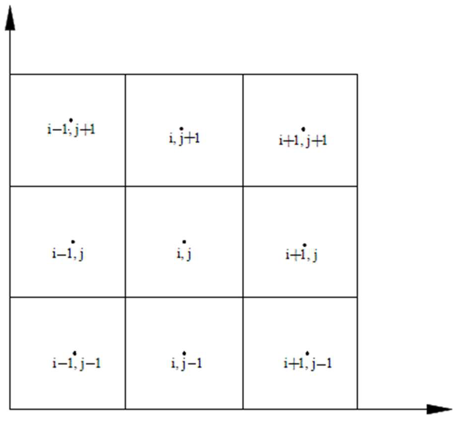
3.1. Discretization of the Shallow-Water Equation

Previous work led by Ferrari [49] demonstrates that the influence of the bed friction and source terms on the simulation of the dam-break problem is often negligible in the 2D dam break, but in 1D, its significance depends on the specifics of the case. The two-dimensional homogeneous equation is

$$U_t+F{\left(U\right)}_x+G{\left(U\right)}_y=0$$

(4)

The general integral form of Equation (4) is expressed as follows:

$$∯(Udxdy-Fdtdy-Gdtdx)=0$$

(5)

By applying the Green’s theorem to Equation (4) and adding the source term, the result becomes

➢

In the x-direction

$$U_{i,j}^{n+1/4}=U_{i,j}^n+\frac{\Delta t}{\Delta x}\left[F_{i+1/2,j}^n-F_{i-1/2,j}^n\right]+\frac{\Delta t}{2}(gh{(S_{ox}-S_{fx})}_i^n+gh{(S_{ox}-S_{fx})}_i^{n+1/4})$$

(6)

➢

In the y-direction

$$U_{i,j}^{n+2/4}=U_{i,j}^{n+1/4}-\frac{\Delta t}{\Delta y}\left[G_{i,j+1/2}^n-G_{i,j-1/2}^n\right]\frac{\Delta t}{2}(gh{(S_{oy}-S_{fy})}_j^{n+1/4}+gh{(S_{oy}-S_{fy})}_j^{n+2/4})$$

(7)

where $U_{i,j}^n$, $U_{i,j}^{n+1/4}$ denote the average solution of U in cells i and j at time level n and n + 1/4, respectively, and $\Delta t$ is the time-step. The spatial intervals $\Delta x$ and $\Delta y$ are the width of the cells i,j in the x and y direction, respectively. $F_{i\pm 1/2,j}^n$ and $G_{i,j\pm 1/2}^n$ are the approximations to the physical fluxes function F(U) and G(U), respectively, from Equation (4).

Godunov-type methods use the Riemann problem to compute the approximations of the fluxes function $F_{i\pm 1/2,j}^n$ and $G_{i,j\pm 1/2}^n.$

3.2. The Riemann Problem

The Riemann problem is solved using Roe’s numerical method, a method widely used in 1D and 2D shallow equations to determine the flow [50]. Roe and Toro [51,52] propose the following formula:

$$F=\frac{1}{2}\left(F_L+F_R-\left|A_e\right|\Delta U\right)$$

(8)

The fluxes computed at the left and right sides are expressed by $F_L$ and $F_{R,}$ respectively; A_e is the Jacobian matrix of F vector at the vertical direction in the boundary and can be evaluated as

$$\left|A_e\right|=\frac{\partial F}{\partial U}=R\left|A\right|W$$

(9)

Matrices R, W, and A can be expressed as

$$R=\left[\begin{array}{ccc}0& 1& 1\\ -n_y& \widehat{u}+\widehat{c}{n}_x& \widehat{u}+\widehat{c}{n}_x\\ n_x& \widehat{v}+\widehat{c}{n}_y& \widehat{v}+\widehat{c}{n}_y\end{array}\right]$$

(10)

$$A=\left[\begin{array}{ccc}\left|\widehat{{\beta }_1}\right|& 0& 0\\ 0& \left|\widehat{{\beta }_2}\right|& 0\\ 0& 0& \left|\widehat{{\beta }_3}\right|\end{array}\right]$$

(11)

$$W=\frac{1}{2\widehat{c}}\left[\begin{array}{ccc}2\widehat{c}\left(\widehat{u}{n}_y-\widehat{v}{n}_x\right)& -2\widehat{c}{n}_y& 2\widehat{c}{n}_y\\ \widehat{c}-\widehat{u}{n}_x-\widehat{v}{n}_y& n_x& n_y\\ \widehat{c}+\widehat{u}{n}_x+\widehat{v}{n}_y& -n_x& -n_y\end{array}\right]$$

(12)

where $n_x$ and $n_y$ are components of the external unit vector in the x and y directions; the eigenvalues are expressed as

$$\widehat{{\beta }_1}=n_x\widehat{u}+n_y\widehat{v}; \widehat{{\beta }_2}=\widehat{{\beta }_1}+\widehat{c}; \widehat{{\beta }_3}=\widehat{{\beta }_1}-\widehat{c}$$

(13)

The average values $\widehat{h},\widehat{u},\mathrm{and}\widehat{v}$ are defined as

$$\widehat{c}=\sqrt{\frac{1}{2}g\left(h_L+h_R\right)}; \widehat{h}=\sqrt{h_R{h}_L} ; \widehat{u}=\frac{\sqrt{{g.h}_L}{U}_L+\sqrt{g.h_R}{U}_R}{\sqrt{{g.h}_R}+\sqrt{{g.h}_L}};\widehat{v}=\frac{\sqrt{{g.h}_L}{v}_L+\sqrt{g.h_R}{v}_R}{\sqrt{{g.h}_R}+\sqrt{{g.h}_L}}$$

(14)

(1)

The MUSCL-Hancock Scheme

The MUSCL-Hancock approach is itself determined via three key steps involving a data-reconstruction step, a step solving the Riemann problem following a direct determination of how the solution evolves in time.

(2)

Data Reconstruction

The data-reconstruction step assesses at the cell’s left and right sides the water depth and velocity. Sanders [27] proposed the following equations:

$$h_L=h_{i,j}+\frac{1}{2}\left(\overline{\Delta h_{i,j}}\right); h_R=h_{i+1,j}-\frac{1}{2}\left(\overline{\Delta h_{i+1,j}}\right)$$

(15)

$$V_L=V_{i,j}+\frac{1}{2}\left(\overline{\Delta V_{i,j}}\right) ; V_R=V_{i+1,j}-\frac{1}{2}\left(\overline{\Delta V_{i+1,j}}\right)$$

(16)

here $V_L$ and $V_R$ are the average cell velocity of the left and right of interface, respectively, and $h_L$ and $h_R$ are the average cell height of the left and right of interface, respectively.

(3)

Time Evolution

The computation grid for the 1D and 2D shallow-water equations consist of boundary and interior cells discretized in the flow direction x and y. The x and y direction are labeled by i = 1, 2, 3 … M and j = 1, 2, 3, … N (see Figure 1). This approach takes into account two ghost cells at all sides, for i = −1, 0 and i = M + 1 and j = −1, 0 and j = N + 1; also, the computation made in the ghost cell should be based on data in the interior cells, namely

$$\begin{gathered} U_{-1,j}^{n+1}=U_{0,j}^{n+1}=U_{1/2,j}\mathrm{and} U_{M+1,j}^{n+1}=U_{M+2,j}^{n+1}=U_{M+1/2,j}, \\ {U}_{i,-1}^{n+1}=U_{i,0}^{n+1}=U_{i,1/2}\mathrm{and} U_{i,N+1}^{n+1}=U_{i,M+2}^{n+1}=U_{i,M+1/2}, \end{gathered}$$

(17)

The head-flow boundary is expressed using $U_{M+1,j}^{n+1}=U_{M+2,j}^{n+1}=\left(\begin{array}{c}{H}_{M+1/2,j}\\ V_{M+1/2,j}\end{array}\right)$ and $U_{i,N+1}^{n+1}=U_{i,N+2}^{n+1}=\left(\begin{array}{c}{H}_{i,N+1/2}\\ V_{i,N+1/2}\end{array}\right)$.

3.2.1. Rusanov Scheme

The resolution of the Riemann problem in edge space steps the solution forward using the Rusanov Scheme as

$$F=\frac{1}{2}\left(F_L+F_R-S_{max}(U_R-U_L\right)$$

(18)

On each side of the edge, namely $U_L$ and $U_R$ are the left and right states of the conservative variables and where the parameter S_max has been developed in [52] as

$$S_{max}=max\left(\left[\left|u_L+\sqrt{g{h}_L}\right|, \left|u_R+\sqrt{g{h}_R}\right|\right]\right)$$

(19)

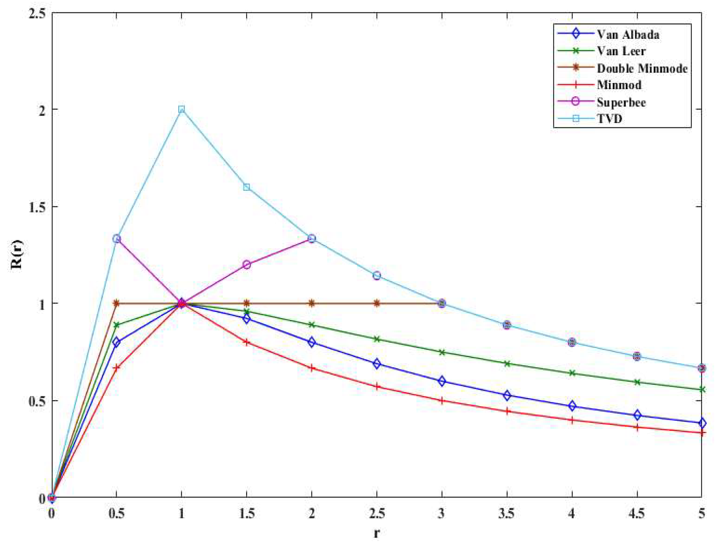
3.2.2. Slope Limiter

The intermediate boundary extrapolation in both the x and y directions is used to compute the conservative variables at the left and right side of the cell as follows:

$$\begin{gathered} U_{i+1/2,j}^L=U_{i,j}+\frac{1}{2}R\left(r_{i+1/2,j}\right)\left(U_{i,j}-U_{i-1,j}\right) \\ {U}_{i+1/2,j}^R=U_{i+1,j}-\frac{1}{2}R\left(r_{i+1/2,j}\right)\left(U_{i+2,j}-U_{i+1,j}\right) \end{gathered}$$

(20)

Here, the subscripts L and R represent the left and right side of the cell, respectively; the cell indices are expressed using the subscripts i and j; $R\left(r_{i+1/2,j}\right)$ is the slope limiter; and $r_{i+1/2,j}$ is computed as

$$r_{i+1/2,j}=\frac{\Delta U_{i+1/2,j}}{\Delta U_{i-1/2,j}}$$

(21)

with

$$\Delta U_{i-1/2,j}=U_{i,j}^n-U_{i-1,j}^n; \Delta U_{i+1/2,j}=U_{i+1,j}^n-U_{i,j}^n$$

(22)

where n denotes the time level.

The resolution of the second-order shallow-water equation through the finite volume method is required by the use of the slope limiters. These slope limiters play an important role in that resolution [33,53,54,55]. Sanders [54] pointed out that the slope limiter evaluates the cell-average gradients of the variables to preserve the monotonicity of the solution at discontinuities (Figure 2). They defined R(r) as the slope limiter; r = $r_{i+1/2,j}$ is the dimensionless ratio between $\Delta U_{i+1/2,j}$ and $\Delta U_{i-1/2,j}$ Equation (21) and gave the following condition for r ≥ 0, then $R\left(r\right)\le \mathit{min}\left(4r/\left(1+r\right),4/\left(1+r\right)\right)$ which satisfies the TVD. When r < 0, all limiters are equal to zero [55]. The expressions of the slope limiter’s formula are as follows:

(1)

Van Albada

$$R\left(r\right)=\frac{2(r+\left|r\right|)}{{\left(1+r\right)}^2}$$

(23)

(2)

Van Leer

$$R\left(r\right)=\frac{2r}{1+r^2}$$

(24)

(3)

Double Minmod

$$R\left(r\right)=\mathit{min}\left(1, \frac{4r}{1+r}, \frac{4}{1+r}\right)$$

(25)

(4)

Minmod

$$R\left(r\right)=\mathit{min}\left(\frac{2}{1+r}, \frac{2r}{1+r}\right)$$

(26)

(5)

Superbee

$$R\left(r\right)=max\left[\mathit{min}\left(\frac{4r}{1+r},\frac{2}{1+r}\right), min\left(\frac{2r}{1+r},\frac{4}{1+r}\right)\right]$$

(27)

The overall numerical process is obviously quite involved with several possible choices to be made along the way. However, the simulation is quite robust even with a challenging problem such as that associated with dam break, as the following results make clearer.

3.2.3. Courant Number

The Courant number is a dimensionless value, representing the time a particle stays in one mesh cell and should be less than or equal to 1. It is computed as follows:

$$CFL=\frac{\Delta t}{min\left\{\frac{\Delta x,\Delta y}{{(C+\sqrt{u^2+v^2})}_{i,j}}\right\}}$$

(28)

where $u$ and v are the characteristic wave speed, $\Delta t$ is the time-step of the numerical model, and $\Delta x$, $\Delta y$ are again the grid spacing. $C=\sqrt{gh}$ is the celerity, and the CFL number is fixed at 1 for the simulation.

4. Results and Discussion

4.1. 1D Dam-Break Simulation

A comparative study is conducted between the numerical models and the theoretical results for different case studies. The first case presents a simulation of a dam break with a dry bed on a short channel (50 m), while the second case analyzes a simulation of a dam break with a dry and wet bed on a long channel (2000 m). The third case presents a simulation of a dam break with a trapezoid obstacle located at the downstream of the dam, which involves the source term.

4.1.1. Computation of the Water Depth: Test 1

To explore the properties of the proposed computational framework, a frictionless horizontal channel with 50 m length is first considered. The dam is located 20 m upstream of the channel. The thickness of the dam is initially neglected, while the upstream water depth is set to 10 m, with a computational space step of 0.5 m and a time step of 0.8 s. With nominal values 0.1 m of the downstream water height is considered as dry. Note that in this section the “theoretical results” are obtained from Bai [29].

Figure 3 shows the comparisons between the theoretical results (solid line) and the two numerical schemes. With a Minmod limiter, an inflection (x = 18 m) and discontinuity point at 31 m can be seen in the simulation (Figure 3a). Van Leer (Figure 3c) and Van Albada (Figure 3d) limiters highlight better results than others; a strong agreement between the two numerical models is observed. The gap between the theoretical and the other two models is very small at the inflection and discontinuity points.

The Superbee (Figure 3b) and double Minmod (Figure 3e) limiters display good agreement between the two models and the theoretical results at the inflection point, but a small difference appears at the discontinuity. The concavity obtained with the Roe scheme is smaller than Rusanov (0.18 and 0.17 m respectively) in the Van Leer limiter (Figure 3c). The simulation based on the first-order equation reveals that the Rusanov scheme is poorer than the Roe scheme (Figure 3f).

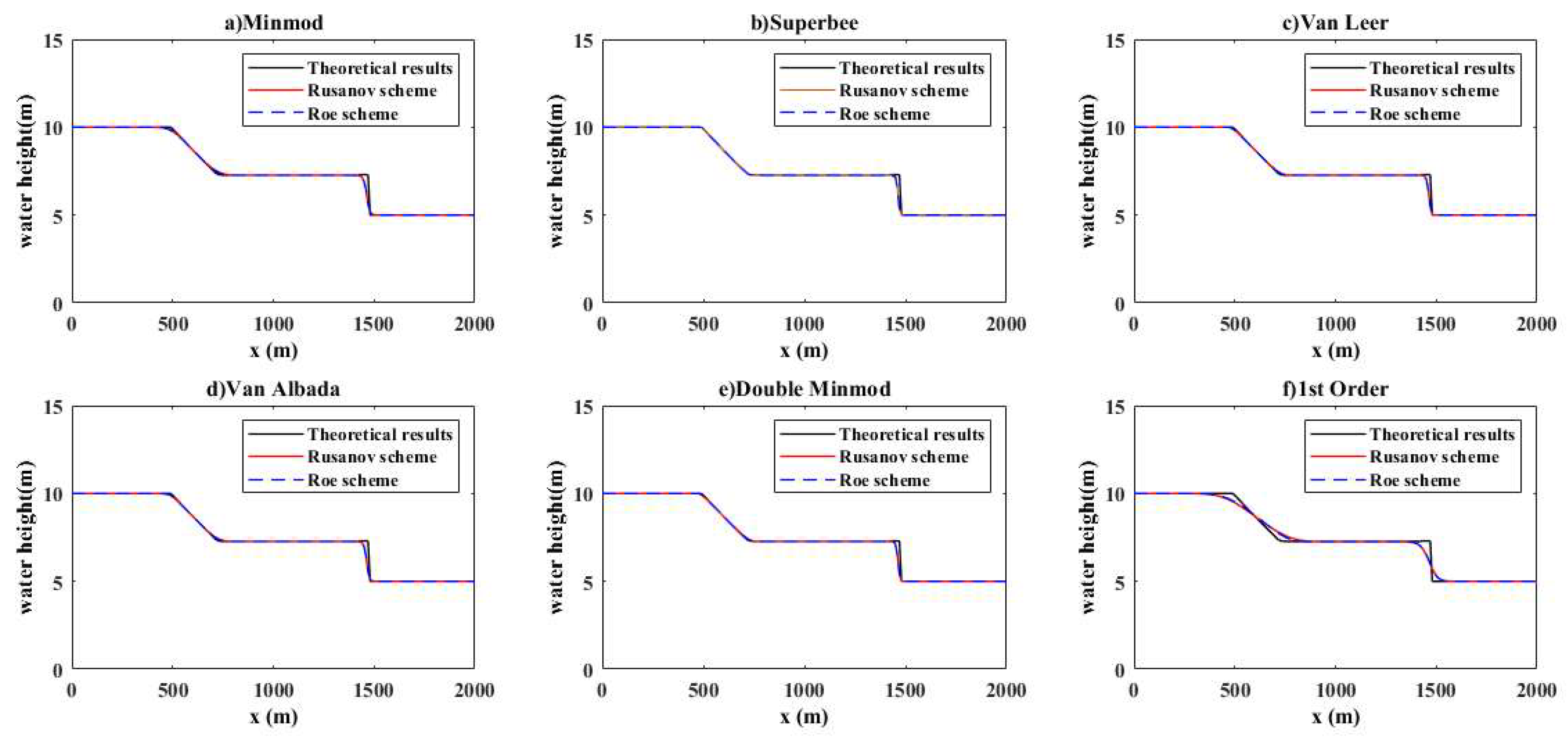
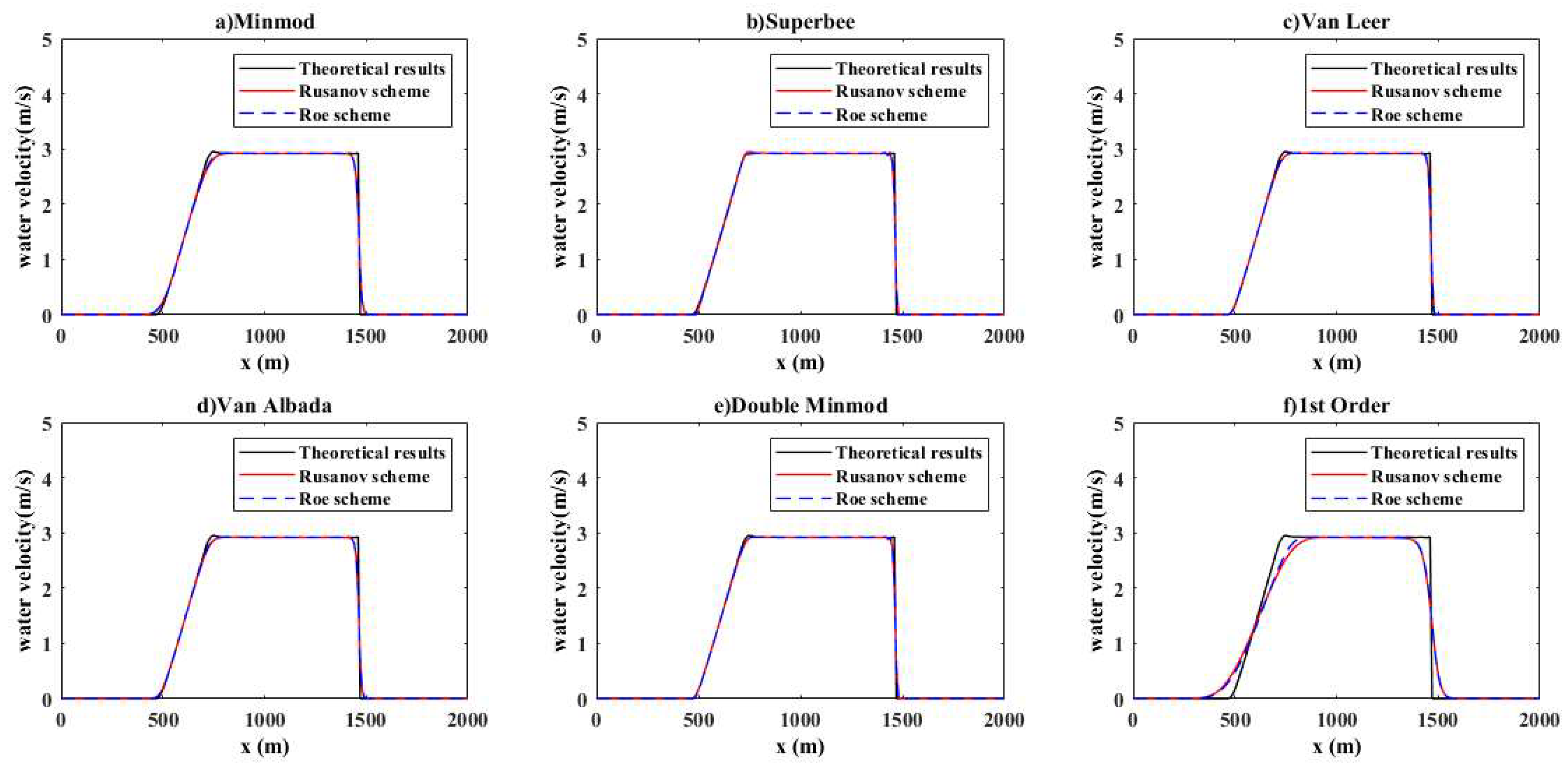
4.1.2. Computation of the Water Depth and Velocity: Test 2

A horizontal channel with friction is simulated, with L = 2000 m and the dam located at 1000 m. The water height upstream was 10 m, with the downstream values varying from 5 m (wet bed case) to 0.1 m for the dry bed [56].

(1)

Water depth

Considering different limiters, the simulations conducted in the case of the wet bed (5 m) with 2000 m as a channel length give the following results: the Minmod limiter (Figure 4a) indicates a slight difference between the two models and the theoretical results at the first (x = 500 m) and second (x = 550 m) inflection points, but the gap widens at the third inflection point (x = 1500 m).

The two models show good agreement with the theoretical results for both the Superbee (Figure 4b) and double Minmod (Figure 4e); a small difference is observed at the third inflection (x = 1500 m).

The limiters of Van Leer and Van Albada (Figure 4c,d) also show good agreement with the theoretical results, although a small gap appears at the third inflection. The gap observed at the third point between the same solution and the two models is higher with Van Leer and Van Albada than the ones using double Minmod and Superbee. The two models do not fully reproduce the theoretical results of the first-order equation (Figure 4f). The gaps are observed at different inflection points. The case of the dry bed (0.1 m) with the channel length which remains 2000 m is analyzed in this part. Firstly, it can be observed that Roe and Rusanov schemes do produce reasonable results with different slope limiters for the 2000 m long channel.

Simulations display a small gap, with the Minmod limiter (Figure 5a) at the inflection point (x = 600 m) and the third inflection (x = 1700 m). The Van Leer and Van Albada limiters (Figure 5c,d) show excellent agreement between the two numerical models with the theoretical results. The results retain their accuracy until the third inflection point, where a small discrepancy arises.

In Figure 5b,e, reasonable results are obtained with Superbee and double Minmod. The difference between the two models and the theoretical results can be observed at the second inflection, and that gap is more significant with the Superbee than the double Minmod limiter. The Roe scheme presents a better result than the Rusanov scheme when the equations are solved in the first order (Figure 5f).

The simulations reveal small discrepancies with the Minmod limiter (Figure 5a) at the inflection point (x = 600 m) and the third inflection (x = 1700 m). The Van Leer and Van Albada limiters (Figure 5c,d) show an excellent pairing between the two numerical models and the theoretical results. The results are quite accurate until the third inflection point, where a small gap appears between the numerical models and the theoretical ones. In Figure 5b,e, strong results can also be obtained with the Superbee and double Minmod methods. The difference between the two models and the theoretical results can be observed at the second inflection point, and that gap is somewhat more significant with the Superbee than the double Minmod limiter. The Roe scheme is slightly better than the Rusanov scheme, at least for first-order models (Figure 5f).

(2)

Water velocity

In the case of a wet bed with different limiters, consistent results are summarized in Figure 6. The flow velocity computed with the second-order of the shallow-water equation at different slope limiters shows strong agreement between the Roe scheme, the Rusanov scheme, and the theoretical results.

Figure 6b,e, reveals that the Superbee and double Minmod provide quite good results. Some minimal discrepancies can be observed at the second (x = 700 m) and third (x = 1500 m) inflection points. The gap between the models and theoretical results at different inflection (4) points are more prominent with the Minmod limiter (Figure 6a).

Van Leer and Van Albada limiters used in (Figure 6c,d) also show quite good results with some minimal gaps at the second and third inflection between the models and the theoretical results. The resolution of the first-order equation does not provide good results but suggests a fair adhesion between the theoretical results and the Roe scheme (Figure 6f).

In a dry bed case (h_l = 0.1 m), the flow velocity is also determined, and the results are displayed in Figure 7, again with good agreement between the two models. In these different figures, Van Leer and Van Albada limiters (Figure 7c,d) reasonably reproduce the theoretical results. A strong agreement between the models and the theoretical results is also observed with Superbee and double Minmod (Figure 7b,e) despite the appearance of an oscillation at the second inflection (x = 1400 m). The height of the oscillation is higher with Superbee than the one with double Minmod. The results are also acceptable with Minmod limiters (Figure 7a), although a small gap is observed at the second (x = 1400 m) and third (x = 1700 m) inflection.

The difference between the two models is more substantial for the case of the dam break with a shorter channel length (50 m). In the case of a dam break with a fairly long channel length (2000 m), the results obtained from the simulation, based on the theoretical results, are accurate and reliable. The simulated height and water velocity compare nicely with the theoretical results. But the model presents defaults for the short lengths (50 m) of the canal, especially for the dry beds (0.1 m). The difference between the simulated value and the theoretical results are greater when the dry bed becomes smaller (0.01 m). The reason for this difference may result from not considering certain parameters such as the friction coefficient or infiltration or the number of cells.

The determination of the CPU time for the case study not only highlights the differences between the two models but also confirms that the Roe scheme tends to be more accurate than the Rusanov approach. The hardware used in calculating the different CPU times is a laptop Asus i7-3537U CPU at 2.00 GHz 2.50 GHz, a 64-bit operating system, and an x64-based processor and that computer was purchased in Nanjing, Jiangsu province in the People’s Republic of China.

Table 1. Computation of the CPU time (s) for test 2.

Limiter	Roe Scheme (hr = 5 m)	Roe Scheme (hr = 0.1 m)	Rusanov Scheme (hr = 5 m)	Rusanov Scheme (hr = 0.1 m)
Minmod	8.249	7.926	8.208	8.048
Superbee	8.139	7.907	8.106	8.130
Van Leer	7.967	7.969	8.104	8.017
Van Albada	7.987	8.119	8.174	8.091
Double Minmod	8.257	8.321	7.931	8.289
1st Order	8.037	8.225	8.147	8.237

summarizes the CPU time for test 2.

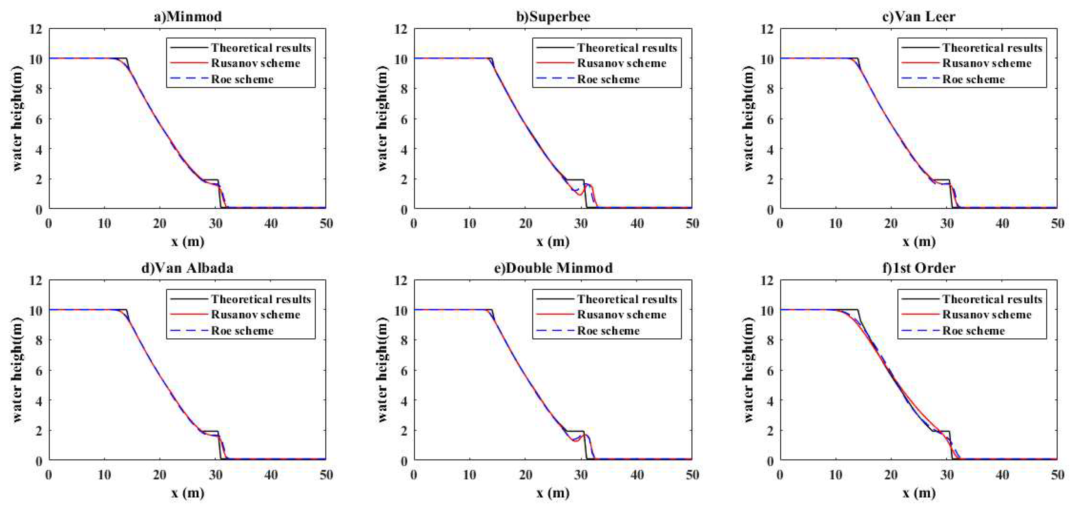
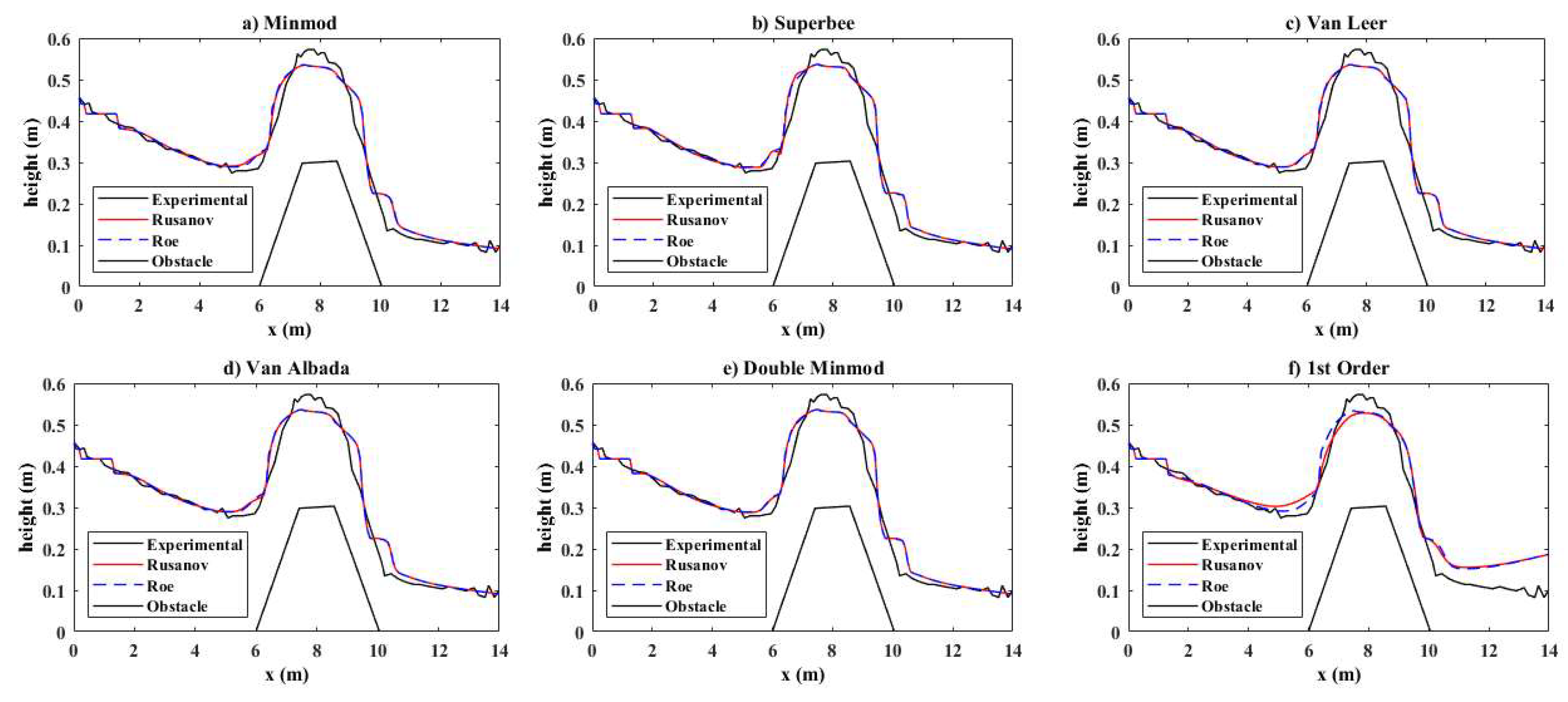
4.1.3. Dam Break over a Trapezoid Obstacle: Test 3

This third test addresses a comparative study between the numerical model and the experimental data of dam-break flow over a dry bed with a trapezoid bottom as an obstacle. The dam is located right at the upstream boundary of the channel where the spatial domain is defined as [−465, 425], the simulation duration has been chosen as T = $41.84/\sqrt{g/h_l}$, and the initial water height is

$$h\left(x,0\right)=\left\{\begin{array}{c}{h}_l=25, if 465\le x\\ h_r=0, otherwise\end{array}\right.$$

(29)

and

$$u\left(x,0\right)=0.$$

(30)

Additionally, $\Delta x=2.5$; $\Delta t=0.002\Delta x$ and the topography is defined using an isosceles trapezoid which has 30 m as its length, a height of 7.5 m, and a base length of 100 m. The topography equation is expressed as follows [57,58]:

$$z\left(x\right)=\left\{\begin{array}{c}\frac{7.5}{35}\left(x-153\right), if 153\le x\le 188\\ 7.5, if 188\le x\le 218\\ 7.5-\frac{7.5}{35}\left(x-218\right), if 218\le x\le 253\\ 0, otherwise \end{array}\right.$$

(31)

The water depth h and the horizontal distance x are non-dimensionalized by the initial water depth ho. The duration of the simulation has been chosen as T = 11.9 s, and the results are illustrated in the Figure 8.

The Rusanov and Roe schemes show a shift compared to the experimental data when the first wave from the dam impacts the base of the obstacle. A second discrepancy is observed after impact in which the experimental curve is generally higher than the simulated values.

The CPU time (

Table 2. CPU time (s) for the dam break with trapezoidal obstacle.

Limiters	Roe Scheme	Rusanov Scheme
Minmod	50.384	50.646
Superbee	50.311	51.093
Van Leer	50.378	50.800
Van Albada	50.337	50.349
Double Minmod	50.968	50.392
First Order	51.188	50.889

) computed for the two models shows that the second-order Roe scheme with Minmod (Figure 8a), Superbee (Figure 8b), Van leer (Figure 8c), and van albada (Figure 8d) is slightly faster than with the Rusanov results. The two models show additional divergence with experimental values after the obstacle particularly for the first-order models (Figure 8f).

The results obtained during the CPU Time calculation for the case of dam break with an obstacle, shows that the Roe scheme is much better than the Rusanov scheme. Table 2 presents the results of the CPU time for a dam break with a trapezoidal obstacle.

The results related to the dam break obtained in the framework of the first part are all for one dimension. The first study on the partial failure of a dam with an asymmetric breach was carried out by Alcrudo [24]. This study has been referenced by many researchers to validate their models.

Having considered one-dimensional simulation results, a two-dimensional study of dam failure is addressed in the next section by again using the Finite volume method–Godunov type with the Roe scheme.

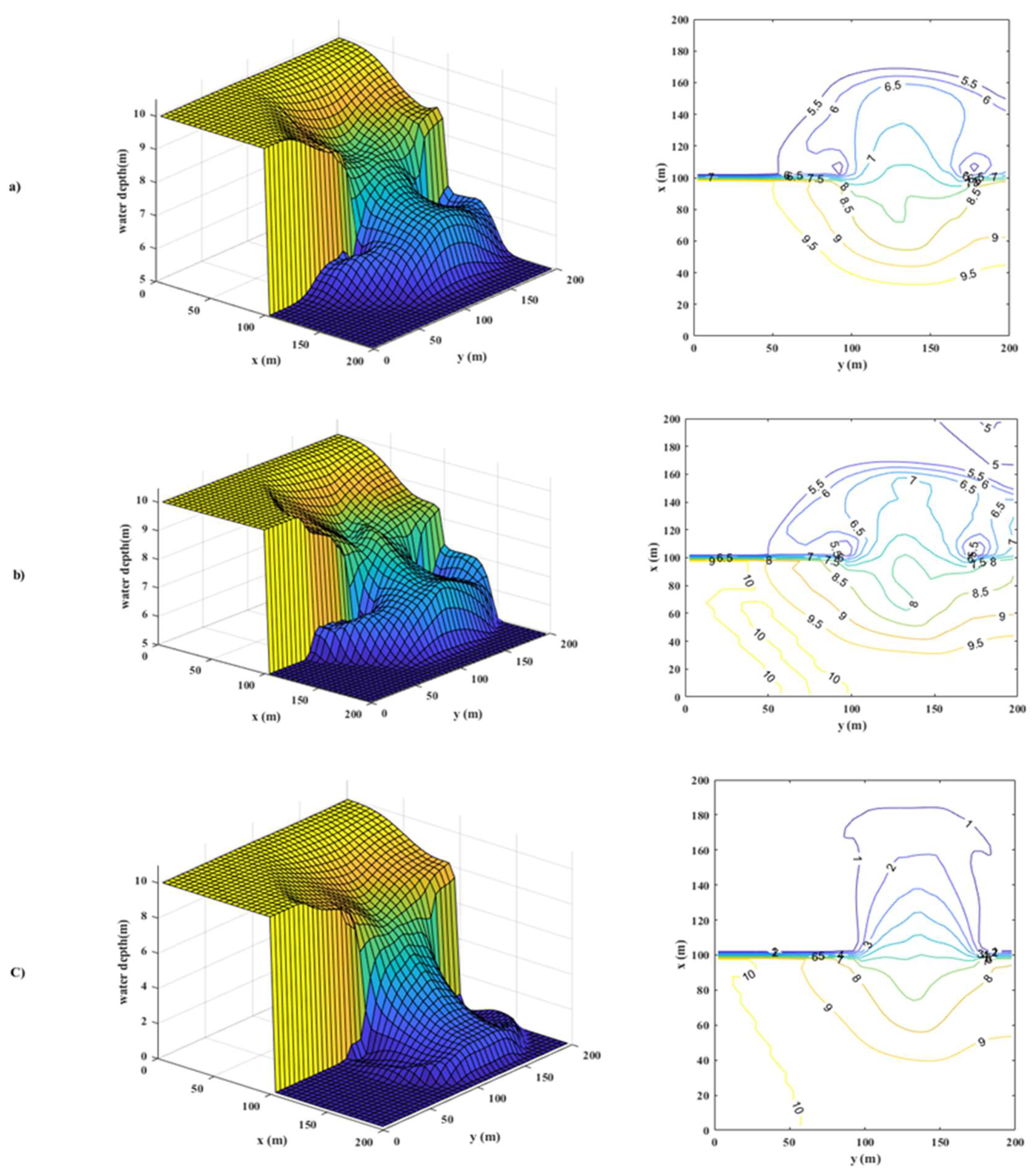
4.2. 2D Dam-Break Simulation

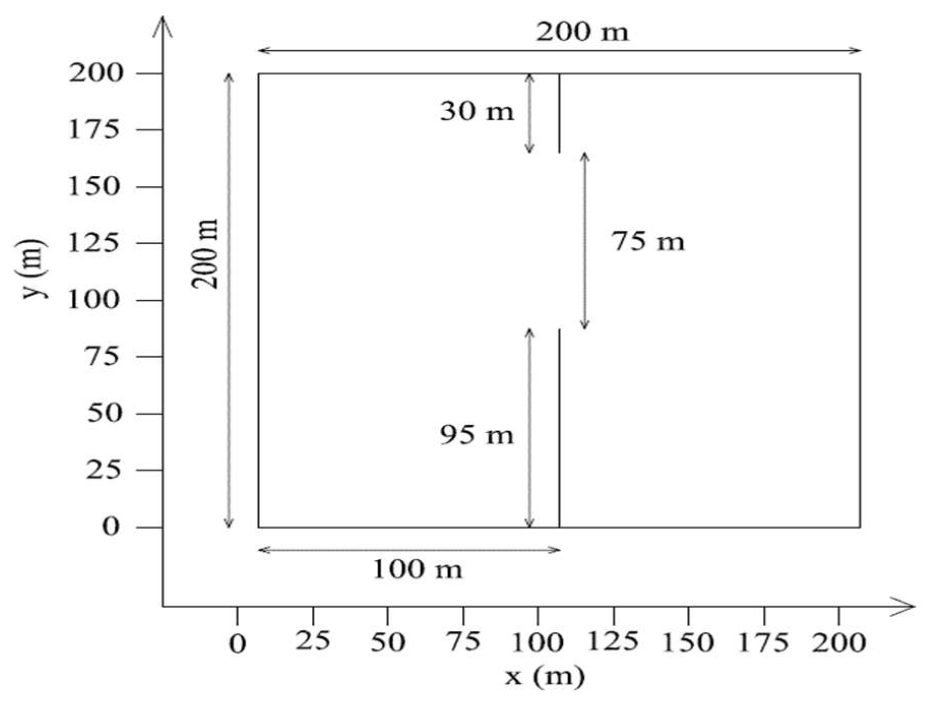
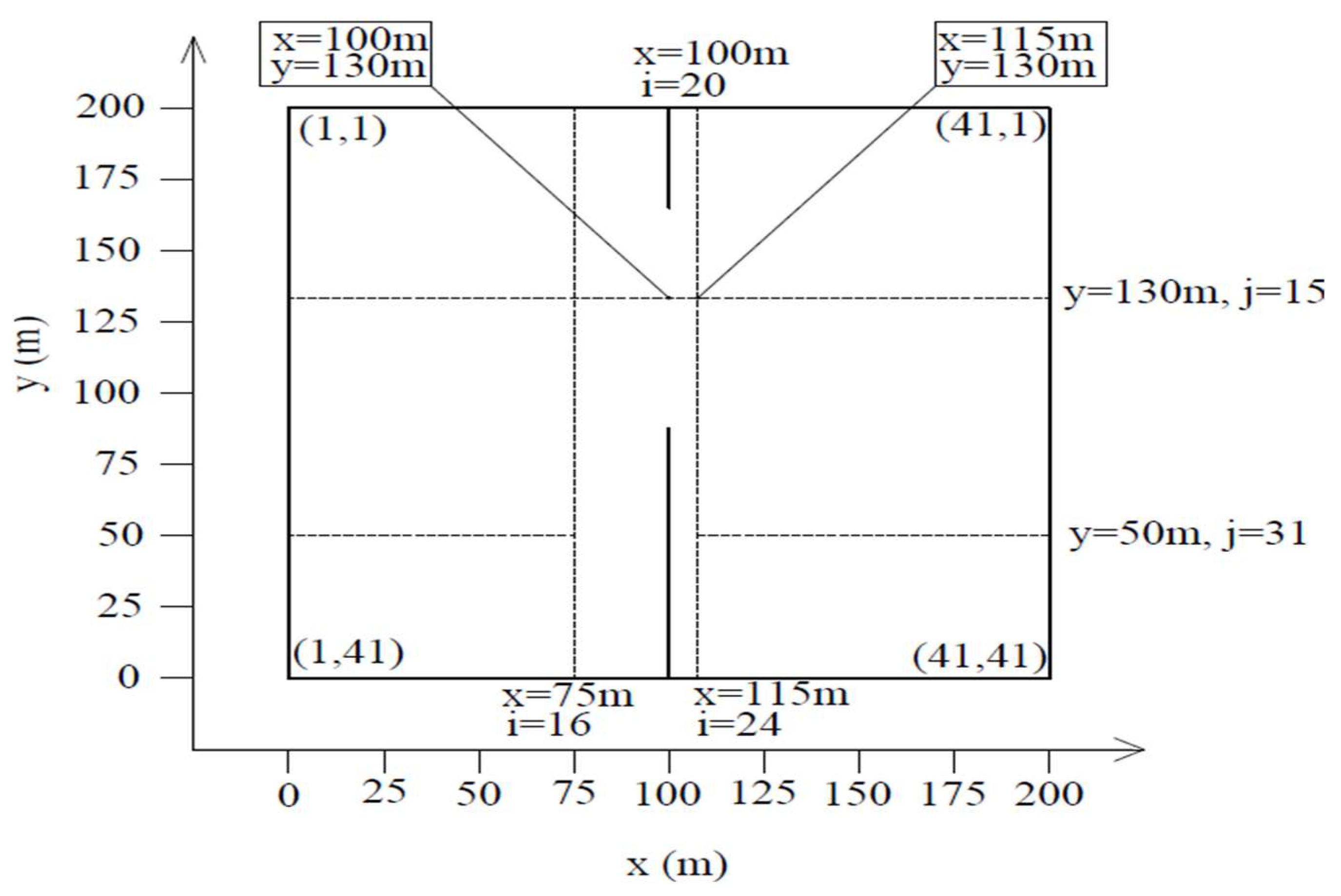
4.2.1. Description of the Study Case

A study is carried out on a dam 200 m wide, 200 m long, and with a frictionless bottom (nm = 0). The water is retained upstream of the dam, namely 200 m in width and 100 m in length. After a sudden rupture of the dam, the breach is 75 m in length which is 30 m from the left bank and 95 m from the right. Figure 9 gives an illustration.

4.2.2. Initial and Boundaries Conditions

The water depth upstream of the dam is H = 10 m; downstream is assumed to be either h = 5 m for the wet bed and 0.1 and 0 m for the dry. The computational domain is a 200 m × 200 m region which has been subdivided into 40 × 40 rectangular grids. A “non-slip” condition is imposed on all walls. The time of the simulation is settled as 7.2 s.

➢

The reflective boundary condition is applied at i + 1/2 of the cell and the equations are given using

$$h\left(i+1,j\right)=h(i,j)u\left(i+1,j\right)=-u(i,j)$$

(32)

$$h\left(i+2,j\right)=h(i-1,j)u\left(i+2,j\right)=-u(i-1,j)$$

(33)

where h, u, and v are the water height, the velocity at the x and y direction, respectively.

➢

In the liberty boundary condition, the borders do not enforce any coercion. That means

$$u\left(i-1,j\right)=u(i,j)$$

(34)

➢

In the periodicity boundary condition, the left and right borders are connected.

$$u\left(1,j\right)=u(n+1,j)$$

(35)

$$u\left(i,1\right)=-u(i,n+1)$$

(36)

✓

First-Order partial Dam Break

The 2D partial-dam-break problem is solved using the Roe scheme and the results are compared to those collected by Zoppou, Delis, and Vosoughifar [7,47,59]. Although the calculation methods are different, the emphasis should be on the contour lines and the shape of the dam.

In the case of rupturing dams with a wet bed (5 m) and a dry bed (0.1 m), the contours are nearly identical to those obtained by Vosoughifar [59] for the first case, but were not previously published for the case of a dry bed (0 m). Meanwhile, the shape of the dam after sudden rupture is similar to that proposed by Zoppou and Delis [7,47] for the three cases (Figure 10a–c), namely wet (5 m) and dry bed (0.1 m and 0 m). The first-order 2D dam-break simulation was conducted for wet bed and dry bed cases. During the simulation, the CPU time was calculated, and the results are presented in

Table 3. CPU time (s) for the first-order 2D dam-break simulation.

Water Depth at Downstream	CPU Time (s)
Wet bed (5 m)	30.534
Dry bed (0.1 m)	30.765
Dry bed (0 m)	30.875

.

The CPU times recapitulated in Table 3 show an increase with the water height downstream of the dam. The maximum value of the CPU time is obtained when the water level downstream of the dam is high and that decreases with a reduction in this water level.

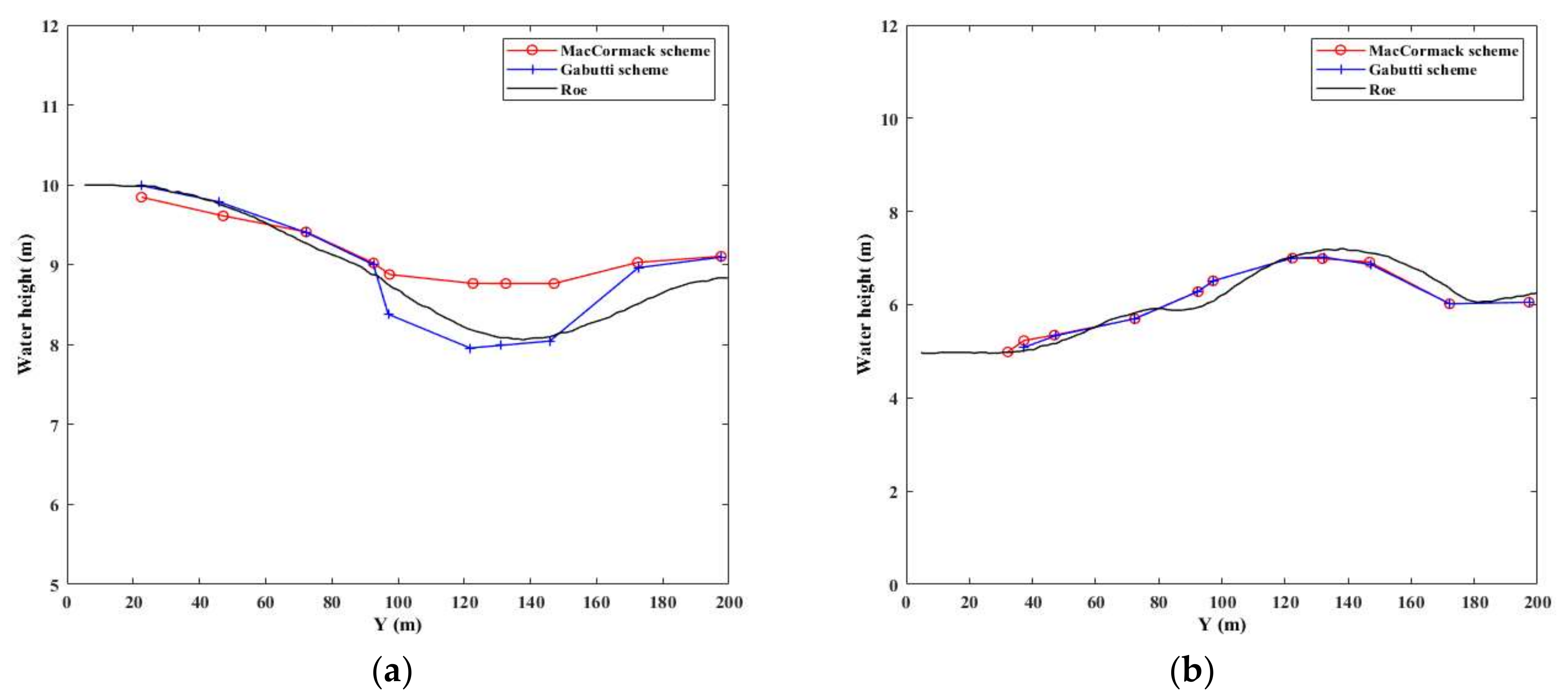
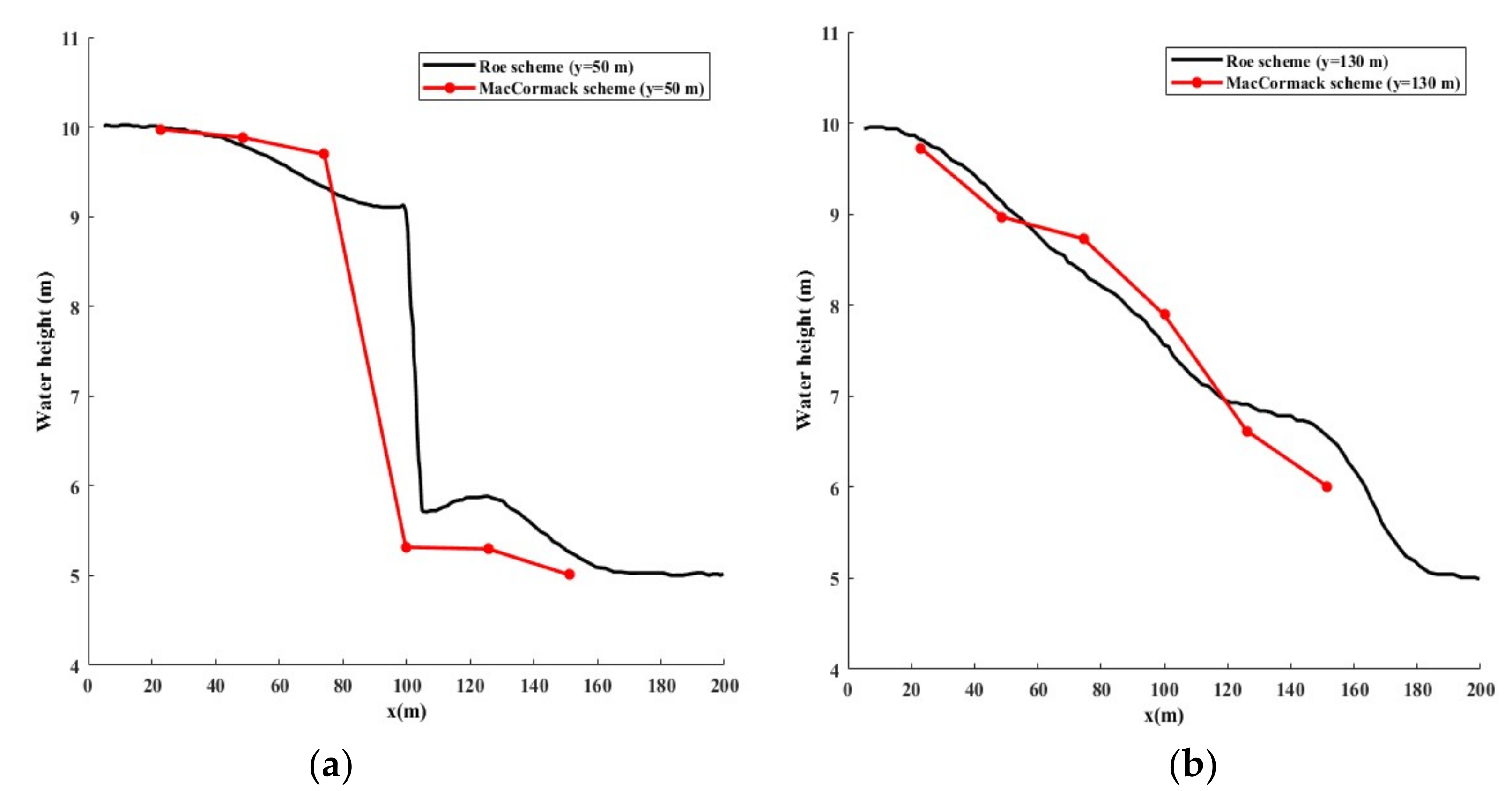
4.3. Transverse and Longitudinal Profiles

In this study, the profiles of some points located throughout the dam are analyzed. A few points are chosen with coordinates and are mentioned in Figure 11.

The results of the cross-sectional profiles obtained as a result of the simulation for a duration of 7.2 s are illustrated in Figure 12. The red line shows the MacCormack’s results, the blue line Gabutti’s, and the black line the Roe scheme results. A comparison between the three simulated results is conducted when the ratio of downstream/upstream is very small. The published literature suggests that Gabutti provides very good results until the downstream/upstream ratio is < 0.2, while MacCormack is generally accurate until a downstream/upstream ratio falls less than 0.25. The current comparison is for the case of a wet bed, and the simulation agrees closely with Gabutti’s results; it is the most robust approach between the two schemes [24,60].

Figure 12a shows the results obtained for a point located at x = 75 m. The figure suggests a fairly good comparison between Gabutti’s result and the Roe scheme results. The results of MacCormack are very close to the Roe scheme results at the start of the simulation, up to y = 110 m before deviating completely. At point x = 115 m (Figure 12b), the results of MacCormack and Gabutti are almost identical and are alternatively close to the Roe scheme results.

Figure 13 illustrates the results of a comparative study between the longitudinal profiles of two points located, respectively, at y = 50 m (Figure 13a) and y = 130 m (Figure 13b), obtained with the Roe scheme simulation (black line), and those produced using the MacCormack scheme (red line).

For y = 50 m (Figure 13a), it appears that the two schemes are identical at the start of the simulation and then diverge at x = 50 m and meet again at the point x = 90 m; the trend of the two curves is in good agreement. When y = 130 m (Figure 13b), the two curves alternately cross throughout the simulation but have an almost identical trend. Strong similarity between the results is obtained from the simulation of two schemes (the Roe and the MacCormack scheme), with slight differences depending on the details of the method of calculation, including the size and shape of the grids.

✓

Second-Order partial Dam Break

The results of the second-order model are shown and compared, with various slope limiters, will be compared to those developed by Delis [47] as follows: Superbee and Minmod limiters for a wet bed (5 m) and Van Leer limiter for two dry bed cases (0.1 m and 0 m).

Figure 14a,b shows the water height as well as the height contours after a simulation of 7.2 s for the case of a dam break with a wet bed (5 m); the Minmod and Superbee are taken as slope limiters. The results obtained within the framework of this study present some differences from those in the literature, particularly in the level of contours. The shapes of the curves are almost identical, but there are some small differences in the trend. Figure 14c present the water height and contours obtained after a simulation of 7.2 s for the case of a dam break with a dry bed (0.1 m). The case is analyzed with Van Leer as the slope limit. The water height obtained from the simulation is similar to those produced by the researchers in their previous studies on the same subject, but the difference always arises in the level of the tendency of the contours. The CPU time from the second-order 2D dam-break simulation is shown in

Table 4. CPU time (s) for the second-order 2D dam-break simulation.

Slope Limiters	Water Depth of Downstream (m)	CPU Time (s)
Minmod	5	10.645
Superbee	5	12.321
Van Leer	0.1	9.564

. This table presents the results for the cases of the Minmod, Superbee, and Van Leer methods.

The results of Table 4 show that the Superbee as the slope limiter provides the greatest value compared to the others; the Van Leer appears much better than the Minmod, although the cases are different, particularly when comparing the wet and dry beds.

The origin of this difference can arise, not only from the calculation method, and the size and shape of the grids, but particularly from the boundary conditions used which can be reflective only, or transmissive, or a combination of both. Within the framework of this study, the rectangular grids of 40 × 40 were considered with a non-slip condition applied to the walls as well as a slip condition permitted at the breach.

Overall, the presented models can simulate the cases of dam failure with a wet bed (5 m) and dry bed (0.1 and 0) as well as to better track the shock wave which arises from the start of the break until the end of the simulation. Simulations relating to the physical form as well as the related contours are approximately similar to those obtained in past studies. The ratio between the downstream/upstream heights for points located on either side of the dam are accurately calculated with excellent agreement with those of existing models such as the Gabutti and MacCormack models.

5. Conclusions

Open channel simulations are critically important, whether they are used for ecological, economic, or legal purposes; thus, many numerical procedures have been developed to address the issues of water depth, velocity, and event sequencing. Some of the most promising of these methods are tested here, using the challenging and important dam-break problem. The dam-break problem is itself important and an excellent numerical test case of the various proposed approaches for solving the flow equations. This work considers the influence of various slope limiters on the dam-break simulation and of the finite volume method with a Godunov-type model with both first- and second-order precision. Theoretical data are compared to simulated results and the stability and calculation accuracy of the second-order model of both the Roe and Rusanov schemes are explored. The dam-break problem admits many possible variations: long and short channel lengths; dry and wet beds; and being with or without an obstacle at the downstream position. The influence of the different slope limiters is analyzed for each case. Moreover, the comparison between the theoretical and the Roe and Rusanov schemes is explored in the case of a 1D dam break. Furthermore, the Roe scheme is then used to simulate the 2D dam break.

The simulations allow the following conclusions to be provisionally stated:

(1)

It is established that the proposed second-order approaches with Rusanov and Roe schemes accurately reproduce the theoretical results better than the first-order model. However, the Roe scheme with Van Leer schemes is slightly more accurate when predicting flow events in various combinations of the two schemes and five slope limiters. The Roe scheme with Van Leer is robust and is recommended for further investigations of the dam-break flow.

(2)

It confirmed that as the channel length and the ratio of downstream water height increase Van Leer, Minmod, and Van Albada do not distort the results; however, in the case of Superbee and double Minmod some non-physical oscillations are observed at the second inflection point.

(3)

When the channel is relatively long, the proposed second-order Godunov–finite volume method with Roe and Rusanov schemes accurately reproduce the water height and velocity for a dam-break flow for both dry and wet bed cases. When using the first-order Godunov–finite volume method, the Roe scheme appears to be more accurate and thus seems ideal for predicting the dam-break flow, and by extension many other less-demanding flows that are highly significance.

(4)

Two models only weakly reproduce the theoretical results when using the second-order schemes with Minmod, Superbee, Van Leer, Van Albada, and double Minmod. This is true both at the level of the first point of contact between the obstacle and the failure wave but also at the top of the obstacle. Not surprisingly, the results in the second order are better than those of the first-order schemes. The Roe scheme appears to be slightly more numerically efficient than the Rusanov scheme.

(5)

The case of the 2D dam-break simulation reveals a greater approximation with the results obtained using the Gabutti scheme than with those of MacCormack. This reflects the capacity of the model to track the shock wave resulting from the sudden dam rupture.

(6)

The second-order precision of the 2D partial dam-break problem with Minmod, Superbee, and Van Leer as slope limiters reveals that the Minmod, Van Leer, and Van Albada slope limiters can be more strongly recommended for further investigations than the Superbee approach.

Future work might include other variations. For example, infiltration might be considered, as well as wider variations in boundary conditions and, crucially, in the dam-failure mechanism. Numerical extensions such as the multilayer shallow-water equations or hyperbolic shallow-water moment equations are possible avenues for further study. However, the overriding consideration is that the dam-break realities pose a much greater risk to humans and property than could ever be captured using a numerical model.

References

1. Wilby, R.L.; Keenan, R. Adapting to flood risk under climate change. Prog. Phys. Geogr. 2012, 36, 348–378. [Google Scholar] [CrossRef]
2. Gao, J.; Ji, C.; Liu, Y.; Gaidai, O.; Ma, X.; Liu, Z. Numerical study on transient harbor oscillations induced by solitary waves. Ocean Eng. 2016, 126, 467–480. [Google Scholar] [CrossRef]
3. Gao, J.; Ma, X.; Chen, H.; Zang, J.; Dong, G. On hydrodynamic characteristics of transient harbor resonance excited by double solitary waves. Ocean. Eng. 2021, 219, 108345. [Google Scholar] [CrossRef]
4. Yanmaz, A.M.; Beser, M.R. On the Reliability-Based Safety Analysis of the Porsuk Dam. Turkish. J. Eng. Environ. Sci. 2005, 29, 309–320. [Google Scholar]
5. Singh, V. Dam Breach Modelling. In Technology; Springer: Dordrecht, The Netherlands, 1996; Volume 17. [Google Scholar]
6. Feng, Z.Y. The seismic signatures of the surge wave from the 2009 Xiaolin landslide-dam breach in Taiwan. Hydrol. Process 2012, 26, 1342–1351. [Google Scholar] [CrossRef]
7. Zoppou, C.; Roberts, S. Numerical solution of the two-dimensional unsteady dam break. Appl. Math. Model. 2000, 24, 457–475. [Google Scholar] [CrossRef]
8. Cornwall, W. Catastrophic failures raise alarm about dams containing muddy mine wastes. Science 2020, 20. [Google Scholar] [CrossRef]
9. American Society of Civil Engineers. Report of the Committee on the Cause of the Failure of the South Fork Dam. Trans. Am. Soc. Civ. Eng. 1890, 24, 448–451. [Google Scholar]
10. Pohle, F.V. The Lagragian Equations of Hydrodynamics: Solutions Which Are Analytic Functions of Time. Ph.D. Thesis, New York University, New York, NY, USA, 1950. [Google Scholar]
11. Saint-Venant, A.B. Théorie et equations générales du movement nonpermanent des eaux courantes. Comptes Rendus Séances l’Académie Sci. Paris Fr. Séance 1871, 17, 147–154. [Google Scholar]
12. Cunge, J. Practical Aspects of Computational River Hydraulics; Pitman Publishing Ltd.: London, UK, 1980; Volume 420. [Google Scholar]
13. Yang, J.; Hsu, C.; Chang, S. Computations of free surface flows Part 1: One-dimensional dam-break flow. J. Hydraul. Res. 1993, 31, 19–34. [Google Scholar] [CrossRef]
14. Scardovelli, R.; Zaleski, S. Direct numerical simulation of free-surface and interfacial flow. Ann. Rev. Fluid. Mech. 1999, 31, 567–603. [Google Scholar] [CrossRef]
15. Chanson, H. The Hydraulics of Open Channel Flow. An Introduction, 2nd ed.; Elsevier: London, UK, 2004. [Google Scholar]
16. Hirsch, C. Numerical Computation of Internal and External Flows, Fundamentals of Numerical Discretization; John Wiley & Sons: New York, NY, USA, 1988; Volume 2. [Google Scholar]
17. Shi, H.D.; Liu, Z. Review and progress of research in numerical simulation of dam-break water flow. Adv. Water Sci. 2006, 17, 129–135. [Google Scholar]
18. Sanders, B.F.; Bradford, S.F. Impact of limiters on accuracy of high-resolution flow and transport models. J. Eng. Mech. 2006, 132, 87–98. [Google Scholar] [CrossRef]
19. Hirsch, C. Numerical computation of internal and external flows. In Computational Methods for Inviscid and Viscous Flows; John Wiley & Sons: Chichester, UK, 1990; Volume 2. [Google Scholar]
20. Bradford, S.F.; Sanders, B.F. Finite-Volume Model for Shallow-Water Flooding of Arbitrary Topography. J. Hydraul. Eng. 2002, 128, 289–298. [Google Scholar] [CrossRef]
21. Zhou, L.; Wang, H.; Bergant, A.; Tijsseling, A.S.; Liu, D.; Guo, S. Godunov-type solution with discrete gas cavity model for transient cavitating pipe flow. J. Hydraul. Eng. 2018, 144, 04018017. [Google Scholar] [CrossRef]
22. Vila, J.P. Schemas Numeriques en Hydraulique des Ecoulements avec Discontinuities. In Proceedings of the XII Congress IAHR, Lausanne, Switzerland, 5 November 1987. [Google Scholar]
23. Godunov, S.K. A Finite Difference Method for the Numerical Computation of Discontinuous Solutions of the Equations to Fluid Dynamics. Mat. Sb. 1959, 47, 271–290. [Google Scholar]
24. Fennema, R.J.; Chaudhry, M.H. Explicit methods for 2-D transient free-surface flows. J. Hydraul. Eng. 1990, 116, 1013–1034. [Google Scholar] [CrossRef]
25. Valiani, A. Un modello numerico semiimplicito per la trattazione di bruschi transitori in moti a superficie libera e fondo mobile. In Proceedings of the 23_ Convegno di Idraulica e Costruzioni Idrauliche, Florence, Italy, 31 August–4 September 1992; Volume E, pp. 261–276. [Google Scholar]
26. Alcrudo, F.; Garcia-Navarro, P. A high-resolution Godunov-type scheme in Finite Volume for the 2D shallow-water equations. Int. J. Numer. Meth. Eng. 1993, 16, 489–505. [Google Scholar] [CrossRef]
27. Sanders, B.F. High-resolution and non-oscillatory solution of the St. Venant equations in non-rectangular and non-prismatic channels. J. Hydraul. Res. 2001, 39, 321–330. [Google Scholar] [CrossRef]
28. Le Touze, C.; Murrone, A.; Guillard, H. Multislope MUSCL method for general unstructured meshes. J. Comput. Phys. 2015, 284, 389–418. [Google Scholar] [CrossRef]
29. Bai, F.P.; Yang, Z.H.; Zhou, W.G. Study of total variation diminishing (TVD) slope limiters in dam-break flow simulation. Water Sci. Eng. 2018, 11, 68–74. [Google Scholar] [CrossRef]
30. Nogueira, X.; Cueto-Felgueroso, L.; Colominas, I.; Navarrina, F.; Casteleiro, M. A new shock-capturing technique based on Moving Least Squares for higher-order numerical schemes on unstructured grids. Comput. Meth. Appl. Mech. Eng. 2010, 199, 2544–2558. [Google Scholar] [CrossRef]
31. Gao, J.; Ji, C.; Gaidai, O.; Liu, Y.; Ma, X. Numerical investigation of transient harbor oscillations induced by N-waves. Coast. Eng. 2017, 125, 119–131. [Google Scholar] [CrossRef]
32. Gao, J.; Chen, H.-Z.; Ma, X.-Z.; Dong, G.-H.; Zang, J.; Liu, Q. Study on Influences of Fringing Reef on Harbor Oscillations Triggered by N-Waves. China Ocean Eng. 2021, 35, 398–409. [Google Scholar] [CrossRef]
33. Ata, R.; Pavan, S.; Khelladi, S.; Toro, E.F. A Weighted Average Flux (WAF) scheme applied to shallow water equations for real-life applications. Adv. Water Resour. 2014, 62, 155–172. [Google Scholar] [CrossRef]
34. Hu, L.; Xu, J.; Wang, L.; Zhu, H. Effects of Different Slope Limiters on Stratified Shear Flow Simulation in a Non-hydrostatic Model. J. Mar. Sci. Eng. 2022, 10, 489. [Google Scholar] [CrossRef]
35. Harten, A.; Engquist, B.; Osher, S.; Chakravarthy, S. Uniformly high order essentially nonoscillatory schemes, III. J. Comput. Phys. 1987, 71, 231–303. [Google Scholar] [CrossRef]
36. Zhu, J.; Qiu, J. A new fifth order finite difference WENO scheme for solving hyperbolic conservation laws. J. Comput. Phys. 2016, 318, 110–121. [Google Scholar] [CrossRef]
37. do Carmo, J.S.A.; Ferreira, J.A.; Pinto, L. On the accurate simulation of nearshore and dam break problems involving dispersive breaking waves. Wave Motion 2019, 85, 125–143. [Google Scholar] [CrossRef]
38. Papoutsellis, C.E.; Yates, M.L.; Simon, B.; Benoit, M. Modelling of depth-induced wave breaking in a fully nonlinear free-surface potential flow model. Coast. Eng. 2019, 154, 103579. [Google Scholar] [CrossRef]
39. Zhuang, Z.; Jun, Z.; Chen, Y.; Qiu, J. A new hybrid WENO scheme for hyperbolic conservation laws. J. Comput. Fluids. 2018, 179, 422–436. [Google Scholar] [CrossRef]
40. Zhu, J.; Qiu, J. A new type of modified WENO schemes for solving hyperbolic conservation laws. SIAM J. Sci. Comput. 2017, 39, A1089–A1113. [Google Scholar] [CrossRef]
41. Bello, A.W.; Djara, T.; Assogba, M.K. Solveur de Riemann HLLC pour les équations 2D de Saint Venant et application a l’écoulement dans la lagune de Cotonou. Afr. Sci. 2017, 13, 445–456. [Google Scholar]
42. Yang, R.; Yang, Y.; Xing, Y. High order sign-preserving and well-balanced exponential Runge-Kutta discontinuous Galerkin methods for the shallow water equations with friction. J. Comput. Phys. 2021, 444, 110543. [Google Scholar] [CrossRef]
43. Huang, G.; Xing, Y.; Xiong, T. High order well-balanced asymptotic preserving finite difference WENO schemes for the shallow water equations in all Froude number. J. Comput. Phys. 2022, 463, 111255. [Google Scholar] [CrossRef]
44. Gonzalez-Aguirre, J.C.; Gonzalez Vazquez, J.A.; Alavez-Ramirez, J.; Silva, R.; Vazquez-Cendon, M.E. Numerical Simulation of Bed Load and Suspended Load Sediment Transport Using Well-Balanced Numerical schemes. Commun. Appl. Math. Comput. 2022, 5, 885–922. [Google Scholar] [CrossRef]
45. Toro, E.F.; Castro, C.E.; Vanzo, D.; Siviglia, A. A flux-vector splitting scheme for the shallow water equations extended to high-order on unstructured meshes. Int. J. Numer. Methods Fluids 2022, 94, 1679–1705. [Google Scholar] [CrossRef]
46. Darwis, M.; Abdullah, K.; Mohammed, A.N. Comparative study of Roe, RHLL and Rusanov flux for shock-capturing schemes. Mater. Sci. Eng. 2017, 243, 012007. [Google Scholar] [CrossRef]
47. Delis, A.I.; Katsaounis, T. Numerical solution of the two-dimensional shallow water equations by the application of relaxation methods. Appl. Math. Model. 2005, 29, 754–783. [Google Scholar] [CrossRef]
48. Zhou, L.; Wang, H.; Liu, D.; Ma, J.; Wang, P.; Xia, L. A second-order Finite Volume Method for pipe flow with column. J. Hydro-Environ. Res. 2017, 17, 47–55. [Google Scholar] [CrossRef]
49. Ferrari, A.; Fraccarollo, L.; Doumbser, M.; Toro, E.; Amanini, A. Three-dimensional flow evolution after a dam break. J. Fluids Mech. 2010, 663, 456. [Google Scholar] [CrossRef]
50. Glaister, P. Approximate Riemann solutions of the shallow water equations. J. Hydraul. Res. 1988, 26, 293–306. [Google Scholar] [CrossRef]
51. Roe, P.L. Approximate Riemann solvers, parameter vectors, and differences schemes. J. Comput. Phys. 1981, 43, 357–372. [Google Scholar] [CrossRef]
52. Toro, E.F. Riemann Solvers and Numerical Methods for Fluid Dynamics: A Practical Introduction; Springer: Berlin/Heidelberg, Germany, 2013. [Google Scholar]
53. Wu, W.M.; Marsooli, R. A depth-averaged 2D shallow water model for breaking and non-breaking long waves affected by rigid vegetation. J. Hydraul. Res. 2014, 50, 557–575. [Google Scholar] [CrossRef]
54. Sanders, B.F.; Bradford, S.F. High-resolution, monotone solution of the adjoint shallow-water equations. Inter. J. Numer. Meth. Fluids 2002, 38, 139–161. [Google Scholar] [CrossRef]
55. Van Albada, G.D.; Van Leer, B.; Roberts, W. A comparative study of computational methods in cosmic gas dynamics Upwind and high-resolution schemes. In Upwind and High-Resolution Schemes; Springer: Berlin/Heidelberg, Germany, 1997; pp. 95–103. [Google Scholar]
56. Behiye, N.I. Computer Code Development for Numerical Solution of the Depth-Integrated Shallow Water Equations to Study Flood Waves. Master’s Thesis, Middle East Technical University, Ankara, Turkey, 2015; pp. 47–49. [Google Scholar]
57. Ozmen-Cagatay, H.; Kocaman, S. Dam-Break Flow in the Presence of Obstacle: Experiment and CFD Simulation. Eng. Appl. Comput. Fluid. Mech. 2011, 5, 541–552. [Google Scholar] [CrossRef]
58. Magdalena, I.; Pebriansyah, M.F.E. Numerical treatment of finite difference method for solving dam break model on a wet-dry bed with an obstacle. Results Eng. 2022, 14, 100382. [Google Scholar] [CrossRef]
59. Vosoughifar, H.R.; Dolatshah, A.; Sadat Shokouhi, S.K. Discretization of Multidimensional Mathematical Equations of Dam Break Phenomena Using a Novel Approach of Finite Volume Method. J. Appl. Math. 2013, 2013, 642485. [Google Scholar] [CrossRef]
60. Garcia-Navarro, P.; Alcrudo, F.; Saviron, J.M. 1-D open-channel flow simulation using TVD McCormack scheme. J. Hydraul. Eng. 1992, 118, 1359–1372. [Google Scholar] [CrossRef]
Figure 1. Computational grid. The black dot (*) represents the center of the grid.
Water 16 00950 g001
Figure 2. Curve of the slope limiters.
Water 16 00950 g002
Figure 3. Comparative study of the water height between the Roe and Rusanov schemes and the theoretical results made within the various limiters at t = 0.8 s with a downstream hl = 0.1 m (1st and 5th slope limiters).
Water 16 00950 g003
Figure 4. Comparative study of the water height between the Roe and Rusanov schemes and the theoretical results made within different limiters at t = 50 s with a downstream hl = 5 m (1st and 5th slope limiters).
Water 16 00950 g004
Figure 5. Comparative study of water height between the Roe and Rusanov schemes and the theoretical results data with various limiters at t = 50 s with a downstream hl = 0.1 m (1st and 5th slope limiters).
Water 16 00950 g005
Figure 6. Comparative study of the velocity between the Roe and Rusanov schemes and the theoretical results made within the various limiters at t = 50 s with a downstream hl = 5 m (1st and 5th slope limiters).
Water 16 00950 g006
Figure 7. Comparative study of the velocity between the Roe and Rusanov schemes and the theoretical results data made within the various limiters at t = 50 s with a downstream hl = 0.1 m (1st and 5th slope limiters).
Water 16 00950 g007
Figure 8. Simulation result of dam break over a trapezoid obstacle after T = 11.9 s.
Water 16 00950 g008
Figure 9. Structure of dam break.
Water 16 00950 g009
Figure 10. Water height and height contours for the 2D dam break with (a) wet bed (5 m); (b) dry bed (0.1 m); and (c) dry bed (0 m).
Water 16 00950 g010
Figure 11. Projection of the dam structure in an orthonormal landmark.
Water 16 00950 g011
Figure 12. Cross-sectional profiles at 7.2s for (a) x = 75 m and (b) x = 115 m.
Water 16 00950 g012
Figure 13. Longitudinal profiles at 7.2 s for (a) y = 50 m and (b) y = 130 m.
Water 16 00950 g013
Figure 14. Water height and contours for a dam break with (a) wet bed (5 m) for Minmod limiter; (b) wet bed (5 m) for Superbee; and (c) dry bed (0.1 m) for Van Leer.
Water 16 00950 g014