Abstract
We analyzed hydrological responses to changing climate and land use/land cover (LULC) for the past (1985–2020) and future (2021–2080) in the Chemoga watershed of the Upper Blue Nile Basin. The watershed comprises four agroecological environments: Moist Kolla, Moist Weyna Dega, Moist Dega, and Wet Wurch. Past and projected LULC changes under business-as-usual (BAU) and land conservation (LC) scenarios were utilized. Climate projections from 2021 to 2080, under two Shared Socioeconomic Pathways (SSP2-4.5 and SSP5-8.5), were downscaled from Global Climate Models. Utilizing the Soil and Water Analysis Tool, we assessed impacts on mean annual surface runoff (SR) and evapotranspiration (ET). Maximum and minimum temperatures increased significantly in the past and future climate scenarios, with a significant rainfall increase observed under SSP5-8.5. Historical trends revealed a 16.6% increase in SR and 7% in ET from 1983–2002 to 2003–2020. Under BAU LULC with the SSP2-4.5 (SSP5-8.5) climate scenario, SR increased by 24% (26.1%) and ET by 3.1% (4.4%) from 2003–2020 to 2021–2050, followed by a subsequent SR rise of 13.7% (14.0%) and ET increase of 6.0% (5.7%) from 2021–2050 to 2051–2080. Conversely, the LC LULC with SSP2-4.5 (SSP5-8.5) resulted in a 5.3% (4.2%) SR decrease and ET increase of 9.7% (11.3%) from 2003–2020 to 2021–2050 and a further SR decrease of 1% (0.7%) and 6.1% (6.9%) ET increase from 2021–2050 to 2051–2080. The Moist Kolla agroecology experienced the highest SR increase due to vegetation clearances for commercial farming. Meanwhile, the LC scenario indicated substantial decreases in SR and marginal increases in ET in the Moist Weyna Dega agroecology due to forest restoration on steep slopes. Overall, SR showed greater sensitivity to LULC changes, while ET was more responsive to climate changes. The results emphasize considering diverse agroecological contexts for effective water resource management under changing climate and LULC scenarios.
1. Introduction
The change in land use/land cover (LULC) and the climate are widely recognized as the key drivers that affect watershed hydrological processes [1,2]. Given the increasing global scarcity of water resources, the hydrological responses to LULC dynamics and climate change have become a major focus for the hydrological community [3,4,5]. These drivers can have complex interactions that influence the quantity, quality, and timing of water flows within watersheds [6]. The continued temporal and spatial variations in LULC and climate significantly influence various aspects of the water balance, such as surface runoff, evapotranspiration, groundwater, and sediment load [7].
Alterations in LULC have been noted to substantially impact surface runoff [8,9], streamflow [10,11], flood frequency [12], base flow [8], groundwater replenishment [13], and evapotranspiration [3,8] within a watershed and hydrological cycles in general [14]. The climate also substantially influences the various components of the hydrologic cycle [15]. Variations in precipitation patterns, temperature, and extreme weather events substantially affect water availability, quality, and the natural hydrological balance [16]. In recent decades, global surface temperatures have risen markedly, witnessed through a 1.1 °C increase in surface temperature in 2011–2020 compared to the average for 1850–1900 [17]. From 1991 to 2021, Africa experienced an average warming rate of approximately +0.3 °C/decade, which was more rapid than the +0.2 °C/decade observed from 1961 to 1990 [18]. These increased temperatures contribute to increased evaporation and alterations in precipitation patterns, potentially causing droughts or floods [19].
General circulation models (GCMs) derived from the Coupled Model Intercomparison Project Phase 6, incorporating socioeconomic development scenarios and emission trends have been widely utilized for predicting climate conditions [20]. While these models provide credible projections, their spatial resolution is insufficient for detailed impact assessments [21,22]. Spatial downscaling methods, such as statistical downscaling models [23,24], bridge the resolution gap between GCMs and localized impact models by utilizing large-scale climate variables to condition local climate variables, thereby enhancing the accuracy of downscaled data [25,26]. These downscaled projections are crucial for evaluating the effect of climate change on agriculture and water resources [25].
The Upper Blue Nile Basin (UBNB) is a geographically and hydrologically important region in East Africa, predominantly in Ethiopia. Characterized by diverse geography and high agricultural potential, the UBNB is a crucial source of the Nile River system, providing more than 60% of the Nile River’s water [27]. Indeed, the increasing water demand in the basin [28], combined with anthropogenic activities and climate change impacts, poses complex challenges for water resource management in the region [29,30]. The basin faces challenges such as soil erosion [31] and water-related issues [32]. Numerous studies in the UBNB have examined the impact of either LULC change [33,34,35] or climate change alone on the water balance [36,37,38]. Some recent studies have investigated the separate and combined impacts of change in LULC and climate on the water resources of the UBNB and reported contrasting findings. Studies by [3,39] indicate that the hydrological processes, particularly surface runoff, are affected by the combined effects of LULC change and climate variability, with LULC change being the dominant factor. Conversely, other studies [4,11,40,41] showed that more hydrological impacts from the combination of LULC with climate than the isolated impacts with the impacts of climate change are predominant. These studies collectively emphasize that the impact of changes in climate and LULC on watershed hydrology varies spatially and may either act synergistically or offset depending on watershed characteristics. The hydrological responses to varying climate and LULC changes in the Chemoga watershed, located in the UBNB, have not been studied in detail despite the spatial variations observed in other regions. Moreover, improvements in climate data and projection scenarios of climate models facilitate further investigation.
Here, we examined the hydrological responses to the separate and combined impacts of climate and LULC changes in the Chemoga watershed. We used statistical downscaling models to develop future climate change scenarios, Cellular Automata–Markov models to project future LULC changes, Mann–Kendall and Pettitt tests for climate trends and change point detection, and a Soil and Water Assessment Tool (SWAT) model to examine the separate and combined impact of LULC and climate changes on watershed hydrology.
2. Material and Methods
2.1. Description of Study Area
The Chemoga watershed is situated within the UBNB of Ethiopia. The study watershed is a part of the Choke Mountain watershed, which is a water tower of the UBNB and is renowned as the origin of over 60 rivers and 270 springs [42]. The study watershed encompasses an approximate area of 714 km2, featuring elevations that vary between 1160 and 4000 m above sea level (m a.s.l.). A study area’s geographical coordinates span from 10°0′46″ N to 10°38′43″ N latitude and 37°30′14″ E to 37°50′24″ E longitude. The Chemoga watershed is characterized by complex topography, heterogeneous land features, and diverse agroecological environments [42,43]. The Chemoga watershed consists of four distinct agroecologies, namely Moist Kolla, Moist Weyna Dega, Moist Dega, and Wet Wurch, each characterized by diverse land features such as varying elevations, slopes, local climates, soil types, and the local dynamics of LULC. The areas of these respective agroecological environments are 83 km2, 205 km2, 359 km2, and 67 km2, as depicted in Figure 1. The agroecologies of the watershed under investigation (Figure 1) were derived from the agroecological zonation outlined for the purpose of deciding on soil and water conservation strategies in Ethiopia [44].
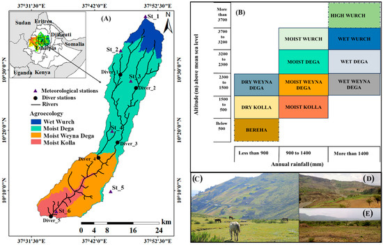
Figure 1.
(A) The location of the study area along with hydrometeorological stations; (B) agroecological zonation system adopted from [44]; (C) photo showing cultivation and settlements on steep terrain in Wet Wurch agroecology; (D) photo showing cultivation over the undulating topography in Moist Weyna Dega; and (E) photo showing the deforestation in the Moist Kolla agroecology.
The long-term mean annual rainfall varied from 1108 mm in Moist Kolla to 1513 mm in Wet Wurch agroecological environments (average 1252 mm). The daily minimum temperature ranged from −1.0 to 8.7 °C at the meteorological stations in Wet Wurch (MS-1) and Moist Kolla (MS-6), respectively (Figure 1). The daily maximum temperature ranged from 15.6 °C at MS-1 to 40 °C at MS-6. The typical characteristics within the four agroecological environments are presented in Table S1 and Figure S1 of the Supplementary Materials.
2.2. Data and Methodology
2.2.1. Land Use/Land Cover Data
LULC datasets were obtained from [42]; see the Supplementary Materials for more detail. The datasets were generated from Landsat satellite images supplemented by 12 aerial photographs with a base scale of about 1:50,000 through the application of a hybrid classification technique that combines unsupervised and supervised techniques. Six LULC types—cropland, woodland, forest, grassland, built-up, and water body—were classified for the years 1985, 1995, 2013, and 2020. Additionally, projections for the years 2040 and 2060 were made using a hybrid Cellular Automata–Markov model under two alternative scenarios: business-as-usual (BAU) and land conservation (LC). These historical and projected thematic maps of LULC were used as the input for the hydrological model (Figure S2). More details concerning LULC classification and future scenario projections of LULC changes are in the Supplementary Materials Sections 1A and 1B, respectively.
2.2.2. Climate Change Scenarios
The majority of climate and hydrological analyses conducted in Ethiopia, particularly in various regions of the UBNB, have relied on existing ground station climate datasets from within the region and neighboring stations. However, these ground stations are often sparse and obtaining meteorological data within small- to medium-sized watersheds (<1000 km2) can be challenging. Fortunately, in the middle of our study watershed (near MS-4 of our installed station), there is one meteorological station that provides long-term climate data. Nevertheless, the agroecological conditions in the watershed vary over short distances [42,43], which complicates the characterization of the entire study area based solely on a single meteorological station.
To validate the presence of varying agroecological settings (Figure 1) and analyze local climate fluctuations in the environments of the various agroecological settings within the study watershed, six automatic weather stations were strategically installed in various watershed areas, taking into consideration the spatial differences in local climate patterns (Figure 1). These weather stations have recorded essential climate data such as rainfall, temperature, and humidity since 2020. We detected spatially diverse climate variables through our installed weather stations (Figure 2). This variability in local climate poses a challenge to utilizing data from established ground stations with long historical records (Figure 2) for drawing conclusions regarding climate and hydrology. For such problems, using satellite climate products is a solution [45]. Therefore, to capture climate variability across different agroecological environments, we utilized spatially gridded datasets from the Enhanced National Climate Time-series Service (ENACTS) in addition to the available climate data from ground stations. ENACTS provides quality-controlled and high-resolution (4 km × 4 km) datasets developed by merging data from ground stations and satellites for Africa [46]. These datasets are more highly correlated both spatially and temporally with ground station data than other available merged datasets including CHIRPS, ARC, and TAMSAT [47]. Abebe [48] evaluated several high-resolution climate data products (i.e., IMERG6, MSWEP2.2, CHIRPS2, and SM2RAIN-ASCAT1.1) within various elevation ranges and reported that the ENACTS dataset develops stronger correlations with ground station data and is more suitable for climate and hydrological studies in UBNB. The observed daily rainfall, minimum and maximum temperature, wind speed, relative humidity, and hours of sunshine as well as the ENACTS grided daily rainfall and maximum and minimum temperature (1983–2018) data were acquired from the National Meteorological Agency of Ethiopia.
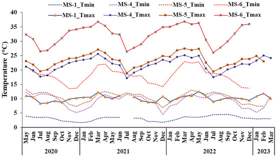
Figure 2.
Local climate variability within different agroecological environments from installed automatic weather stations (MS-1, MS-4, MS-5, and MS-6) (Figure 1). Tmin and Tmax indicate minimum and maximum temperature, respectively.
Future climate data from 2021 to 2080 were downscaled statistically from ten General Circulation Models (GCMs) in the sixth phase of the Coupled Model Intercomparison Project of the Intergovernmental Panel on Climate Change for two Shared Socioeconomic Pathways (SSPs), the SSP2–4.5 and SSP5–8.5 scenarios. The SSP2–4.5 scenario represents a moderate path in which global and national institutions aim for sustainable development goals without exceeding a nominal radiative forcing level of 4.5 W/m2. In contrast, SSP5–8.5 represents a business-as-usual or fossil-fueled development scenario, leading to a nominal radiative forcing level of 8.5 W/m2 by 2100 [20]. From a thorough evaluation of over 31 available GCMs, 10 were carefully selected for downscaling and ensemble use (Table S3), with the primary criteria being the availability on a daily basis of historical and future climate variables, precipitation, and minimum and maximum temperatures, for both SSP2–4.5 and SSP5–8.5 scenarios. For additional details about the General Circulation Models (GCMs) and the methodology employed for downscaling, please refer to Section 2A in the Supplementary Materials.
2.2.3. Streamflow Data
The 1983–2009 streamflow data were obtained from the Ethiopian Ministry of Water, Irrigation and Energy (https://mowe.gov.et/). The streamflow gauging station was located in the middle part of the watershed flow gauging (FG) station (FG-2 in Figure 1). Additionally, we installed four automatic pressure transducer water level recorders called “TD-Divers” (Schlumberger Water Services, The Netherlands) along the Chemoga River and its tributaries labeled FG-1 to -4 (Figure 1). Staff gauges for manual readings were positioned at the same locations as the FG stations. To ensure accuracy, the water levels measured by the pressure sensors were adjusted using the manually recorded water levels from the staff gauges. The current meters and floating method were used for flow velocity measurement at various water stages. Subsequently, discharge rating curves were developed for each station, and the water levels recorded from 2020 to 2023 were converted into discharge values.
Thereafter, the transfer of the long-term streamflow data from station FG-2 to FG-4 was performed. Numerous techniques are available for estimating river flows at ungauged sites, such as regional regression, the area-ratio method, and physically based models. Given the topographical heterogeneity, varying soil types, complex land use dynamics, and other characteristics within the study watershed across the various agroecological environments [42,43], utilizing the abovementioned transfer methods may yield inaccurate results. Hence, instead of relying solely on these transfer methods, we opted to transfer streamflow data by establishing correlation factors derived from recorded data at two stations within the same time spans. These correlation coefficients were then utilized to transfer long-term historical flow data from station FG-2 to FG-4, with separate coefficients developed for the rainy season and dry season (Figure S11).
2.2.4. Spatial Data
A Digital Elevation Model (DEM) with a 30 m resolution was obtained from the USGS website (https://earthexplorer.usgs.gov (accessed on 10 February 2021)) and then projected onto UTM zone 37 using the WGS 1984 data. The DEM was subsequently employed to delineate the study watershed and analyze drainage patterns.
The soil map of the Chemoga watershed with six major soil types (i.e., Haplic Luvisols, Haplic Alisols, Eutric Leptosols, Eutric Cambisols, Eutric Vertisols, and Urban) was acquired from the Ethiopian Ministry of Water, Irrigation and Energy (Figure S1). The physio-chemical properties and textural classes of soil were acquired from soil property maps of Africa with 250 m resolution at six standard depths (0–5, 5–15, 15–30, 30–60, 60–100, and 100–200 cm) accessed from ISRIC–World Soil Information (https://www.isric.org/projects/soil-property-maps-africa-250-m-resolution (accessed on 25 May 2022)). These datasets are high-resolution, reliable, and suitable products available for Africa that have been used by various researchers for the current study region [37,38] and others.
2.2.5. Trend and Change Point Detection of Climatic Variables
The non-parametric Mann–Kendall (MK) [49] test for trend analysis, Sen’s slope estimator [50] for estimation of trend magnitude, and the Pettitt test [51] for change point detection were applied. These models were chosen because of their suitability for non-normally distributed data of hydroclimatic time series [52].
The existence of autocorrelation in time series data may cause the MK test to reject the null hypothesis of no trend detection [53]. To mitigate the influence of autocorrelation when conducting MK trend analysis, we employed a method known as trend-free prewhitening before performing the MK trend test, the most suitable and widely applied technique to remove autocorrelation in hydroclimatic data [54]. The S statistic used for the MK trend test and its variance [49] were calculated as follows:
where xi denotes the independent observations, i is the range from 1 to n, and n is the total number of observations.
The trend magnitude was estimated using the following equation (1968):
where and are the sequential data values. β is considered the median among all conceivable pair combinations within the entire dataset. A β value that is positive indicates an upward trend, whereas a negative β value suggests a downward trend in the time series.
The Pettitt test is used to identify the time at which the shift (change point) occurs by comparing two segments of a time series and evaluating the change in their means. It calculates a test statistic based on the total number of times one observation in the series is greater than another, considering different split points in the data [55]. If the time series data of has a distribution function of the second time series data (, then the data series has a change point.
2.2.6. Hydrological Model Setup
The SWAT model is a spatially distributed, process-based, physically based model designed to analyze how hydrological systems respond to changes in climate, land use, and land management practices within watersheds that vary in size and complexity [56]. The setup and data preprocessing for the SWAT model were carried out utilizing the ArcSWAT2012 tool within the ArcGIS platform (Figure S7). Utilizing the DEM and stream networks, the watershed under investigation was divided into 138 sub-basins, which were then further subdivided into 1872 hydrological response units (HRUs). These HRUs were defined by their consistent attributes related to LULC, soil type, and slope. This detailed subdivision aimed to specifically accommodate hydrological simulations for various agroecological settings within the study watershed. The modified Soil Conservation Service Curve Number method [57] and the Penman–Monteith method were utilized for surface runoff and potential evapotranspiration estimation, respectively. To simulate the hydrological processes, SWAT uses a water balance equation [3,11]:
where (t) is time in days; SW0 (mm) is the content of soil water at the initial time; SWt (mm) is the water content of the soil at the final time; and R, ET, P, and QR are the daily amounts of precipitation, evapotranspiration, percolation, and return flow, respectively; all units are in mm. Qsurf represents the quantity of surface runoff or the surplus rainfall for day i, measured in (mm) (Equation (5)):
S represents the retention parameter (mm):
where CN denotes the curve number for the day. The evapotranspiration was estimated through the Penman–Monteith method.
2.2.7. Hydrological Model Calibration and Validation
Parameter sensitivity analysis, calibration, and validation were conducted using the SWAT-CUP model, employing the Sequential Uncertainty Fitting (SUFI-2) algorithm [58]. The global sensitivity analysis option [59] was utilized to identify the parameters most sensitive to model calibration and validation (Figure S7). Following the selection of these sensitive parameters, adjustments to input parameters were made during the calibration process, with the goal of reducing prediction uncertainty [11].
The daily weather data and monthly streamflow from 1983–2023 were divided into three periods: 1983–1985 for the warm-up period, 1986–2009 for the calibration period, and 2015–2023 for the validation period. Note the absence of streamflow data between 2009 and 2014. We used an extended calibration period to incorporate a wide range of meteorological and hydrological conditions, including both wet and dry years [60]. Calibration was carried out at the watershed outlet. Due to the short-term flow data for stations FG-1–3, we utilized the flow data from these stations for validation purposes. During both the calibration and validation periods, the model’s performance was assessed with essential goodness-of-fit evaluation criteria. The methodological framework we employed for land use/land cover and climate change impact studies on water balance and details of model performance evaluation are found (Figure S7; Section 2A) in the Supplementary Materials.
2.2.8. Evaluation of LULC and Climate Change Impacts on Surface Runoff
To assess the effects on both separate and combined impacts in comparison to the baseline condition, we formulated twenty-eight scenarios by partitioning the climate period into four intervals (Table 1). The criteria to divide the climate periods was based on an analysis of the results obtained from the Pettitt test change point detection applied to both past and future climate variables: the long-term climate dataset was segmented into period-1 (1983–2002), period-2 (2003–2020), period-3 (2021–2050), and period-4 (2051–2080). The details of the change point detection are further discussed in Section 3.1.

Table 1.
Simulated scenarios within the Soil and Water Assessment Tool. The scenarios labeled S-10, S-12, S-14, … correspond to the SSP2–4.5 climate projection scenarios, while S-11, S-13, S-15, … correspond to the SSP5–8.5 scenarios. BAU and LC represent the land use/land cover changes associated with business-as-usual and land conservation scenarios, respectively.
The combined impact of LULC and climate change was assessed by running the calibrated SWAT model using both historical climate data 1983–2002 and 2003–2020 with LULC 1995 and LULC 2013, respectively, and the future ensemble mean of climate variables 2021–2050 and 2051–2080 under the SSP2–4.5 and SSP5–8.5 scenarios with LULC 2040 and 2060, respectively, under the BAU and LC scenarios.
The separate impact analysis was conducted through a “one-factor-at-a-time” method, in which individual factors were modified one at a time while keeping the other conditions constant [3]. The separate impacts from climate and land use/land cover and their combined ( impacts on hydrological processes were estimated using Equations (7), (8), and (9), respectively:
where i represents the simulation numbers (i.e., i = 1, 2, 3, 4, 5 …n) and n denotes the simulation periods.
While there was limited focus on SWC practices in the study watershed, we observed SWC measures like soil bunds in some sub-basins. To address this, SWC practices within the study area were mapped from Google Earth imagery and subsequently validated through on-site field surveys (Figure S8). The parameter values related to the management practices in the SWAT model, specifically curve number (CN2.mgt) values for sub-basins with SWC practices, were modified based on results from the experimental plots [7,61].
3. Results
3.1. Climate Projection and Trend Analysis
The ensemble means of climate variables downscaled from ten GCMs for SSP2–4.5 and SSP5–8.5 scenarios were utilized for trend analysis and to evaluate their impacts on hydrology. The Mann–Kendall trend test was conducted at the 5% significance level on areal average at the watershed level (Table 2) and each of the four agroecological environments was separately considered (Table S4). We found significant increases in maximum temperature and minimum temperature both in the past and future scenarios. Over the last 35 years, maximum and minimum temperatures revealed a significant upward trend, with increases reaching 0.7 °C and 1.7 °C, respectively. The warmer climate in the future is expected to be reflected in 2080 by increases of up to 1.8 °C (2.4 °C) for maximum temperature and 1.8 °C (3 °C) for minimum temperature under SSP2–4.5 (SSP5–8.5). Precipitation did not show consistent patterns in the past and future under SSP2–4.5 while a notable increase by 2080 of 231.6 mm was observed under the SSP5–8.5 climate scenario (Table 2). The patterns and trends of climate variables, both in the past and future climate projections were relatively similar across the agroecological environments with the exception of Moist Kolla agroecology for the past study periods. Moist Kolla agroecology experienced an insignificant trend of maximum temperature with a significant rise in minimum temperature and precipitation in the past.
Table 2.
Mann–Kendall test of trends and Pettitt test of change points in the areal average for Chemoga watershed precipitation and mean, maximum, and minimum temperatures.
For both historical and future climate variables, change points were detected in the annual minimum, maximum, and mean temperatures, and rainfall data (Table 2). In the case of historical climate variables, these change points occurred in 2002, while they occurred in 2050 in the future scenarios (Table 2). Additional information about the results of the MK trend test, Pettitt test, and Sen’s slope estimator can be found in the Supplementary Materials (Table S4; Figures S4–S6).
3.2. SWAT Model’s Sensitivity Analysis, Calibration, and Validation
The SWAT model was initially set up with a 1995 LULC map and climate data for 1983–2020. A global sensitivity analysis was carried out using the SWAT-CUP model on 18 flow parameters (Table S5), resulting in the identification of 10 parameters that were found to be more sensitive for the Chemoga watershed (Table S6). The calibration process utilized monthly observed streamflow data for 1983–2009 with the 1995 LULC map at the FG-4 station (outlet point) (Figure 1), whereas validation was performed for multiple stations (i.e., FG-1, FG-2, FG-3, and FG-4) using streamflow records for 2015–2023 with the 2020 LULC map. The calibration results indicate that the SWAT model can capture the observed flow with R2, NSE, and PBIAS values of 0.83, 0.83, and 5.50, respectively (Table 3, Figure 3). Additionally, the validation results demonstrate favorable agreement with the observed streamflow (Table 3, Figure 4).
Table 3.
Goodness-of-fit statistics for streamflow simulation results during both the calibration period (1983–2009) and the validation period (2015–2023).
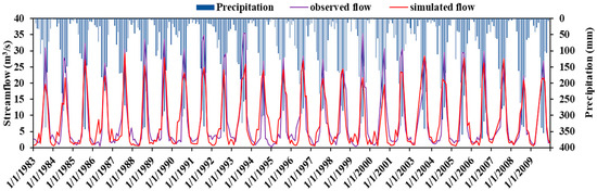
Figure 3.
The monthly streamflow data for both observed and simulated values during the calibration period (1983–2009) of the Chemoga watershed.
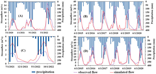
Figure 4.
Observed and simulated streamflow during the validation period (2015–2023) across stations FG-1 (A), FG-2 (B), FG-3 (C), and FG-4 (D).
3.3. Combined Effect of LULC and Climate Change on Surface Runoff and Evapotranspiration
The combined effects of the changes in LULC and climate on surface runoff (SR) and evapotranspiration (ET) were assessed at the watershed scale (Table 4) and across four distinct agroecological environments (Table 5 and Table 6). The watershed-level analysis revealed a substantial increase in mean annual SR of 16.6% from period-1 (1983–2002) to period-2 (2003–2020). This continued with a 24% (26.1%) increase from period-2 to period-3 (2021–2050) and an additional 13.7% (14.0%) increase from period-3 to period-4 (2051–2080) in the SSP2–4.5 (SSP5–8.5) climate combined with the BAU LULC scenario (Table 4; Figure S9). In contrast, with the LC LULC scenario combined with the SSP2–4.5 (SSP5–8.5) climate scenario, the mean annual SR declined by 5.3% (4.2%) from period-2 to period-3 and by an additional 1.0% (0.7%) from period-3 to period-4 (Table 4). ET increased by 7.0% from period-1 to period-2, by 3.1% (4.4%) from period-2 to period-3, and by 6.0% (5.7%) from period-3 to period-4 under the SSP2–4.5 (SSP5–8.5) climate scenarios with the BAU LULC scenario. Under the LC LULC scenario combined with the SSP2–4.5 (SSP5–8.5) climate scenarios, ET increased by 9.7% (11.3%) from period-2 to period-3 and by 6.1% (6.9%) from period-3 to period-4 (Table 4; Figure S10).
Table 4.
Combined and isolated effects of climate change and LULC on mean annual SR (upper) and ET (lower) in the Chemoga watershed. The study periods, labeled as Periods-1, -2, -3, and -4, correspond to the years 1983–2002, 2003–2020, 2021–2050, and 2051–2080, respectively.
Table 5.
The separate and combined effects of climate and LULC change on mean annual runoff within four agroecological environments of the Chemoga watershed. The study periods labeled as Periods-1, -2, -3, and -4 correspond to the years 1983–2002, 2003–2020, 2021–2050, and 2051–2080, respectively.
Table 6.
The separate and combined effects of climate and LULC change on mean annual evapotranspiration within four agroecological environments of the Chemoga watershed. The study periods labeled as Periods-1, -2, -3, and -4 correspond to the years 1983–2002, 2003–2020, 2021–2050, and 2051–2080, respectively.
The analysis considering the four agroecological environments revealed varying trends in the mean annual SR for different LULC and climate change scenarios. The mean annual SR increased when the BAU LULC changes were combined with the two climate scenarios across all the agroecologies; Moist Kolla experienced the highest increase in SR followed by Wet Wurch (Table 5; Figure S9). In Moist Kolla under the BAU LULC change scenario combined with SSP2–4.5 (SSP5–8.5), the mean annual SR substantially increased by 315.9% from period-1 to period-2, by 56.6% (62.8%) from period-2 to period-3, and by an additional 35.2% (38.6%) from period-3 to period-4. Likewise, under the SSP2–4.5 (SSP5–8.5) climate scenarios combined with the BAU LULC change scenario, SR in Wet Wurch increased by 19.2% from period-1 to period-2, by 22.9% (26.1%) from period-2 to period-3, and by an additional 12.1% (14.7%) from period-3 to period-4. In contrast, under the LC LULC change scenario, the mean annual SR substantially decreased across the four agroecological zones with the exception of Moist Kolla. Under the LC LULC scenario, the reduction in SR in Moist Weyna Dega was the highest followed by Moist Dega: in Moist Weyna Dega under the SSP2–4.5 (SSP5–8.5) climate scenarios, SR decreased by 17% (14%) from period-2 to period-3 and by an additional 0.9% (0.7%) from period-3 to period-4. Under the SSP2–4.5 (SSP5–8.5) climate scenarios, SR in Moist Dega decreased by 13.5% (11.6%) from period-2 to period-3 (Table 5; Figure S9).
The combined Impact of LULC and climate change increased ET in all four agroecological environments (Table 6; Figure S10). This rise was observed for both BAU and LC LULC change scenarios and both the SSP2–4.5 and SSP5–8.5 climate scenarios. The increases were greater in the SSP5–8.5 scenario than in the SSP2–4.5 scenario. Moreover, the ET increases under the LC LULC change scenario were greater than under the BAU LULC change scenario (Table 6; Figure S10).
3.4. Isolated Impacts of LULC and Climate Change on SR and ET
At the watershed level, the mean annual SR increased under the separate impact of the BAU LULC change scenario by 12.9% from period-1 to period-2, by 22.6% from period-2 to period-3, and further by 9.5% from period-3 to period-4 (Table 4). In contrast, under the LC LULC scenario, SR decreased by 11.3% from period-2 to period-3 and further decreased by 3.4% from period-3 to period-4. ET decreased in the past and under the BAU LULC change scenario and increased under the LC LULC change scenario. Under the BAU LULC change scenario, ET decreased by 1.8% from period-2 to period-3 and increased by 0.1% from period-3 to period-4. ET increased under the LC LULC change scenario by 5.2% from period-2 to period-3 and by 0.5% from period-3 to period-4.
The separate impacts of climate change on SR and ET showed positive trends both in the past and future study periods. SR increased by 1.2% from period-1 to period-2, by 2.9% (4.3%) from period-2 to period-3, and further increased by 3% (3.7%) from period-3 to period-4 under the SSP2–4.5(SSP5–8.5) climate scenarios. Similarly, ET showed an increase of 9.3% from period-1 to period-2, of 6.5% (7.7%) from period-2 to period-3, and a further increase of 7.6% (6.8%) from period-3 to period-4 under the SSP2–4.5(SSP5–8.5) climate scenarios (Table 4).
The increase in mean annual SR was revealed across the distinct agroecological environments with each exhibiting varying rates of increase under the BAU LULC change scenario (Table 5). The rate of change in the mean annual SR in Moist Kolla agroecology was a severe surge, with a substantial increase of 164.8% from period-1 to period-2, of 41.9% from period-2 to period-3, and a further increase of 23.9% from period-3 to period-4. Following the severe surge in SR in Moist Kolla, Wet Wurch agroecology also witnessed a substantial rise in SR, with a 14% increase from period-1 to period-2, a 16.7% increase from period-2 to period-3, and a subsequent increase of 9.7% from period-3 to period-4. In contrast, SR exhibited a decrease across the distinct agroecological environments under the LC LULC change scenario with the exception of in Moist Kolla agroecology. In Moist Kolla agroecology, the SR increased by 16% from period-2 to period-3, and then slightly decreased by 1.4% from period-3 to period-4 under the separate impact of the LC LULC change scenario. Under this LULC change scenario, Moist Weyna Dega agroecology experienced a substantial reduction in SR with a rate of 24.5% from period-2 to period-3 and a further decrease of 3.3% from period-3 to period-4 compared to other agroecologies.
Considered separately from climate change, the impact of BAU LULC on the mean annual ET was negative for all agroecological environments (Table 6), with the decreases greater in the Moist Kolla agroecological environment than those in the other agroecological zones. In Moist Kolla, ET decreased by 1.2%, 2.6%, and 3.2% from period-1 to period-2, period-2 to period-3, and period-3 to period-4, respectively. In contrast, the mean annual ET increased under the LC LULC change scenario across all agroecological environments (Table 6).
Under the impact of climate change considered separately from changes in LULC, the mean annual SR increased consistently across all four agroecological environments, with higher increases under the SSP5–8.5 climate scenario compared to SSP2–4.5 (Table 5). Likewise, the mean annual ET increased under the separate impacts of the climate change scenarios, with the increases under the SSP5–8.5 climate scenario being greater (Table 6). More information on the hydrological model simulation results for separate and combined impacts of climate and LULC change scenarios on SR and ET both at watershed and distinct agroecological levels is in Tables S7 and S8 of the Supplementary Materials.
4. Discussion
4.1. SR and ET Responses to the Combined Impact of LULC and Climate Change
The combined impact of LULC and climate change differed from their separate impacts depending on the scenarios and hydrological components. The BAU LULC change scenario combined with climate change resulted in a synergistic impact on SR and an offsetting impact on ET. In contrast, the effects of the LC LULC change scenario combined with climate change were offsetting for SR and synergistic for ET. Furthermore, the rate of SR change was predominantly affected by LULC change, rather than climate change. Meanwhile, ET was more impacted by climate change, rather than LULC change scenarios.
The agroecological analysis of the combined impact of BAU LULC and climate change on SR and ET revealed synergistic effects on SR and offsetting effects on ET consistently across the distinct agroecological environments. More specifically, the increased rate of SR under the BAU LULC scenario combined with climate change in Moist Kolla was higher than in the other agroecological environments. The rates of SR increases in Moist Kolla were intense from period-1 to period-2 and then continued increasing. This rapid change is due to the fact that this environment was fully covered with woodland until 1995, after which a dramatic expansion of cropland, particularly for commercial agriculture, led to substantial increases in SR rates. Although the rate of change in SR was high in the Moist Kolla followed by the Wet Wurch agroecological environment, in fact, Moist Dega is characterized by little vegetative cover and extensive cultivated areas subject to high SR over the past long history. The increased SR causes sheet erosion to intensify and rills and gullies to widen and deepen, as observed in the field [42].
The effects of the LC LULC change scenario combined with climate change were offsetting for SR and synergistic for ET across the distinct agroecological environments. Under this combination, the rate of decrease in SR in the Moist Weyna Dega was substantially higher than those in the other agroecological environments, because Moist Weyna Dega is characterized by steep slopes comprising more than 62% of the total area. The synergistic impact of the LC LULC scenario combined with climate change caused ET to increase consistently across all four agroecological environments. Our findings align with those of prior studies conducted in various regions of the UBNB: as the extent of cropland increases, SR increases and ET decreases [3,4,10,41,62,63]. The research conducted by Berihun [3] in lowland, midland, and highland environments in the UBNB found that the counterbalance (offsetting) effect of LULC change to climate change led to a decrease in the ET. Their findings also revealed that the change in LULC change had the dominant role for SR and ET were highly correlated with climate change which is in agreement with our findings. Similarly, the study by Wedajo [63] on the separate and combined impacts of climate and LULC on hydrological components in the Dhidhessa River basin of the UBNB revealed an increase in both SR and ET under their combined effects. SR was more affected by LULC changes, whereas ET was more affected by climate changes. Their study also reported that the combined effects were synergistic and offsetting for SR and ET, respectively. Teklay et al. [41], in their study of hydrological responses to the climate and LULC change in the Gumara watershed of the UBNB under three alternative LULC scenarios (BAU, expansion of forestland, and expansion of irrigated crops) and two climate change scenarios, reported that SR increased under BAU and decreased with increased ET under the other two alternative scenarios. Another study on the projected climate and LULC with alternative scenarios reported that the combined effects of climate and LULC increase both SR and ET under the BAU scenario and reduce SR under management scenarios [62].
4.2. SR and ET Responses to the Impact of LULC Changes
The major changes in LULC were the substantial increases in cropland and built-up areas, accompanied by reductions in grassland and woodland. Future projected LULC change under the BAU scenario indicates a further increase in cropland and built-up areas at the expense of woodland and grassland. The intensive cultivation and reduction in vegetation cover in this watershed have contributed substantially to land degradation, leading to increased SR and decreased ET. As vegetation cover decreases, SR increases, simultaneously reducing transpiration, and leading to decreased ET. With the complex topography of steep to very steep slopes covering more than 30% of the study watershed, SR has substantially increased in the past and is projected to continue increasing into the future. In contrast, the rise in vegetation coverage under the LC LULC change scenario leads to a decrease in SR and an increase in ET. This scenario projects an increase in vegetation cover, particularly over steep and very steep slopes, which would intercept SR, increase transpiration from plants to the atmosphere, and increase ET.
The agroecological-based hydrological analysis revealed more detailed information that can help in designing and implementing effective and sustainable water resource management strategies at the local level. The separate impact of LULC shows a consistent trend of increasing SR and a slight decrease in ET across distinct agroecological environments in the past and continued into the future with projected LULC changes under the BAU scenario. More specifically, the rate of increase in SR was higher in the Moist Kolla followed by the Wet Wurch agroecological environments compared to the other agroecological environments. This intensified SR in the Moist Kolla was aggravated by a substantial increase in cropland at the expense of woodland. This change occurred because of the introduction of commercial farming into the hotter, and less populated areas. Similarly, in the Wet Wurch agroecology, the expansion of cropland over steep and very steep slopes increased the SR change. ET was impacted negatively by LULC changes under the BAU scenario across the four agroecological environments. The substantial reduction in woodland resulted in a decrease in transpiration from plants and decreased ET.
In the LC LULC change scenario, SR decreased in all agroecological environments except in Moist Kolla. The SR decreased because the LC scenario promotes increased vegetation cover over steep and very steep slopes (>15% slope) to facilitate sustainable land management. In Moist Kolla, approximately 82.7% of the area is flat to sloping (<15% slope; Table S1), making it suitable for cropland expansion. This leads to the expansion of commercial farming to this agroecological environment causing the increase in SR under this LC scenario; however, the rate of the SR increase was noticeably lower than that under the BAU scenario. The Moist Weyna Dega agroecological environment experienced the most substantial reduction in SR compared to others under the LC scenario. This agroecology is characterized by 62.8% of its area being under steep to very steep slopes (>15% slope) and the LC scenario projects to increase in vegetation cover over this steep area rather than agricultural use. Moreover, the increase in SR under BAU and the decrease under the LC scenario from period-2 to period-3 were higher compared to the changes from period-3 to period-4. These findings are in accordance with those of previous studies in various parts of the UBNB [7,33,35]. Gashaw [33] studied the hydrological impact of the projected LULC changes under the BAU scenario by 2030 and 2045 in the Andassa watershed of the UBNB; they found increases in both SR and ET. A similar study by Leta [64] in the Nashe watershed of the UBNB reported increases in SR and decreases in ET in the future to 2050. Another study by Bekele [65] in the Ketela watershed of Ethiopia also reported an increase in SR under the impact of LULC changes.
4.3. SR and ET Responses to the Impact of Climate Changes
Both minimum and maximum temperatures in the study watershed have significantly and consistently increased from 1983 to 2020, and they are projected to continue to increase in the future (2021–2080) under the SSP2–4.5 and SSP5–8.5 climate scenarios. Rainfall patterns have been highly variable, with a non-significant increase in the past (1983–2020) and a significant increasing trend in the future, particularly under the SSP5-8.5 climate scenario. Climate change has been observed to be positively correlated with SR and ET. Looking ahead, the projected impact of future climate change on both SR and ET is more pronounced under the SSP5–8.5 climate scenario than SSP2–4.5. In both past and future study periods, there was a consistent relationship between the impact of climate on SR and ET across the studied agroecological environments. Previous studies of the impact of climate change scenarios on watershed hydrology in the UBNB [36,37,60] agreed that SR and ET will consistently increase [38]. Teklay et al. [37] observed significant hydrological changes in the Lake Tana Basin of the UBNB in response to climate change. Their study, conducted under RCP 4.5 and RCP 8.5 climate scenarios, revealed that by 2055, temperatures and rainfall are projected to substantially increase, particularly under the RCP 8.5 emission scenario. Additionally, they noted a significant rise in ET. A similar study by Mengistu [60] in the UBNB also projected a significant increase in temperature with inconsistent patterns of rainfall attributed to an increase in SR of 14% and 27% in ET by the end of the twenty-first century. In contrast, a study by Worku [38] in the Jemma sub-basin of the UBNB revealed a consistent decrease in SR and an increase in ET under both the RCP 4.5 and RCP 8.5 climate scenarios in the twenty-first century. These contrasting results are mainly due to the spatial heterogeneity of LULC changes and climate variability.
5. Conclusions
This study presents an integrated modeling approach for assessing the separate and combined effects of LULC and climatic changes on hydrologic processes in four varied agroecological regions of the Chemoga watershed in Ethiopia. The study used an ensemble mean from ten GCM outputs downscaled for the SSP2–4.5 and SSP5–8.5 climate scenarios. LULC maps from 1985, 1995, 2013, and 2020 along with projected LULC for 2040 and 2060 under BAU and LC LULC scenarios were employed to understand their impacts on hydrological processes across these four distinct agroecological environments.
Both the minimum and maximum temperatures significantly increased, evident in both historical (1983–2020) and future (2021–2080) periods under the SSP2–4.5 and SSP5–8.5 climate scenarios, ranging from 0.02 to 0.05 °C/year. A slight increase in mean annual rainfall was observed in the past, with more substantial increases projected under SSP5–8.5. The combined impact of climate and LULC change during the historical period reveals SR increases of 316%, 15%, 9%, and 19% in Moist Kolla, Moist Weyna Dega, Moist Dega, and Wet Wurch agroecologies, respectively. Similarly, ET increased by 5%, 7%, 8%, and 2%, respectively, in the corresponding agroecological environments. Further SR increases are projected in the near future (2021–2050) and far future (2051–2080). In the respective agroecological environments under the BAU LULC coupled with the SSP2–4.5 (SSP5–8.5) climate scenario, SR in the far future is projected to increase by 38% (45%), 24% (29%), 30% (33%), and 112% (126%) compared to the recent past (2013–2020), while ET is projected to increase by 8% (9%), 9% (11%), 18% (21%), and 16% (22%).
In contrast, the LC LULC scenario combined with the SSP2–4.5 (SSP5–8.5) climate change scenarios result in decreasing SR by 18% (15%), 14% (11%), and 10% (9%), in the Moist Weyna Dega, Moist Dega, and Wet Wurch agroecological environments, respectively, in the far future compared to the observed recent past SR. In general, the LULC changes under BAU combined with the climate change scenarios were synergistic for SR and offsetting for ET, and the LC LULC scenario combined with climate change scenarios had offsetting impacts for SR and synergistic ones for ET. These findings provide essential insights for the sustainable management of natural resources in the Chemoga watershed and other regions facing similar challenges from changes in climate and LULC.
Supplementary Materials
The following supporting information can be downloaded at https://www.mdpi.com/article/10.3390/w16071037/s1: Figure S1. Major soil textures (A), types (B), and slope classes (C) within distinct agroecological regions in Chemoga watershed. Figure S2. Land use land cover maps (left) and areal extent of land use and land cover (LULC) categories (right) at the watershed level and in four different agroecological environments. Figure S3. Suitability map for land allocation to (A) built-up, (B) cropland, (C) forest, (D) grassland, (E) water body, and (F) woodland in the Chemoga watershed. Figure S4. Pettitt’s test for change point detection in historical rainfall (A–D) and future downscaled rainfall under the SSP2-4.5 climate scenario (E–H) and under the SSP5-8.5 climate scenario (I–L) in the Wet Wurch, Moist Dega, Moist Weyna Dega, and Moist Kolla agroecological environments, respectively. Figure S5. Pettitt’s test for change point detection in historical maximum temperature (A–D) and future downscaled maximum temperature under the SSP2-4.5 climate scenario (E–H) and under the SSP5-8.5 climate scenario (I–L) in the Wet Wurch, Moist Dega, Moist Weyna Dega, and Moist Kolla agroecological environments respectively. Figure S6. Pettitt’s test for change point detection in historical minimum temperature (A–D) and future downscaled minimum temperature under the SSP2-4.5 climate scenario (E–H) and under the SSP5-8.5 climate scenario (I–L) in the Wet Wurch, Moist Dega, Moist Weyna Dega, and Moist Kolla agroecological environments, respectively. Figure S7. Methodological framework employed for land use/land cover and climate change impact studies on water balance. The land use/land cover (LULC) datasets utilized in this study were obtained from [2]. Figure S8. Soil and Water Conservation (SWC) practices (bunds with/out grass) identified, along with the corresponding images captured from Google Earth. Figure S9. Mean annual surface runoff (SR) both at the watershed level (on the left) and across four distinct agroecological environments (on the right). Figure S10. Mean annual Evapotranspiration (ET) both at the watershed level (on the left) and across four distinct agroecological environments (on the right). Figure S11. Correlation of streamflow between stations FG-2 and FG-4 in the rainy and dry seasons. Table S1. Typical characteristics of four agroecological environments in Chemoga watershed. Table S2. Factors and constraints considered and their weights for predicting LULC conditions in the Chemoga watershed. Table S3. Global climate models used in this study. Table S4. Mann–Kendall and Sen’s slope results for rainfall (mm/year) and maximum and minimum temperature (°C/year) trends. Table S5. SWAT model parameters with their initial values. Table S6. Final optimized parameter values within the parameter range during the last iteration of calibration. Table S7. The SWAT model simulated results of hydrological responses to the separate and combined impacts of climate and land use/land cover (LULC) changes. Table S8. SWAT model simulated results of hydrological responses to the separate and combined impacts of climate and land use/land cover (LULC) changes in four agroecological environments. References [66,67,68,69,70,71,72,73] are cited in the supplementary materials.
Author Contributions
T.M.M.: Conceptualization; Data Curation; Formal Analysis; Investigation; Methodology; Software; Validation; Visualization; Roles/Writing—Original Draft; Writing—Review and Editing. A.T., N.H., and M.T.: Conceptualization; Funding acquisition; Methodology; Project Administration; Resources; Supervision; Writing—Review and Editing. A.A.F. and M.L.B.: Conceptualization; Data Curation; Writing—Review and Editing. A.M., A.S.B., D.S., K.E., T.A.S., S.B.K., Y.B.H. and, T.A.: Writing—Review and Editing. All authors have read and agreed to the published version of the manuscript.
Funding
This study received collaborative funding from the Science and Technology Research Partnership for Sustainable Development under Grant Number JPMJSA1601, provided by the Japan Science and Technology Agency and Japan International Cooperation Agency. Additionally, support was obtained from Grants-in-Aid for Scientific Research (KAKENHI) under Grant Number JP19K13434, awarded by the Japan Society for the Promotion of Science.
Data Availability Statement
Data are contained within the article and Supplementary Materials.
Conflicts of Interest
The authors declare that they have no known competing financial interests or personal relationships that could have appeared to influence the work reported in this paper.
References
- Chanapathi, T.; Thatikonda, S. Investigating the impact of climate and land-use land cover changes on hydrological predictions over the Krishna River basin under present and future scenarios. Sci. Total Environ. 2020, 721, 137736. [Google Scholar] [CrossRef] [PubMed]
- Chawanda, C.J.; Nkwasa, A.; Thiery, W.; van Griensven, A. Combined impacts of climate and land-use change on future water resources in Africa. Hydrol. Earth Syst. Sci. 2024, 28, 117–138. [Google Scholar] [CrossRef]
- Berihun, M.L.; Tsunekawa, A.; Haregeweyn, N.; Meshesha, D.T.; Adgo, E.; Tsubo, M.; Masunaga, T.; Ayele Almaw Fenta, A.A.F.; Dagnenet Sultan, D.S.; Mesenbet Yibeltal, M.Y.; et al. Hydrological responses to land use/land cover change and climate variability in contrasting agro-ecological environments of the Upper Blue Nile basin, Ethiopia. Sci. Total Environ. 2019, 689, 347–365. [Google Scholar] [CrossRef] [PubMed]
- Getachew, B.; Manjunatha, B.R.; Bhat, H.G. Modeling projected impacts of climate and land use/land cover changes on hydrological responses in the Lake Tana Basin, upper Blue Nile River Basin, Ethiopia. J. Hydrol. 2021, 595, 125974. [Google Scholar] [CrossRef]
- Tsegaye, L.; Bharti, R. The impacts of LULC and climate change scenarios on the hydrology and sediment yield of Rib watershed, Ethiopia. Environ. Monit. Assess. 2022, 194, 717. [Google Scholar] [CrossRef] [PubMed]
- Li, X.; Zhang, Y.; Ma, N.; Li, C.; Luan, J. Contrasting effects of climate and LULC change on blue water resources at varying temporal and spatial scales. Sci. Total Environ. 2021, 786, 147488. [Google Scholar] [CrossRef]
- Berihun, M.L.; Tsunekawa, A.; Haregeweyn, N.; Tsubo, M.; Fenta, A.A.; Ebabu, K.; Sultan, D.; Dile, Y.T. Reduced runoff and sediment loss under alternative land capability-based land use and management options in a sub-humid watershed of Ethiopia. J. Hydrol. Reg. Stud. 2022, 40, 100998. [Google Scholar] [CrossRef]
- Das, P.; Behera, M.D.; Patidar, N.; Sahoo, B.; Tripathi, P.; Behera, P.R.; Srivastava, S.K.; Roy, P.S.; Thakur, P.; Agrawal, S.P.; et al. Impact of LULC change on the runoff, base flow and evapotranspiration dynamics in eastern Indian river basins during 1985–2005 using variable infiltration capacity approach. J. Earth Syst. Sci. 2018, 127, 19. [Google Scholar] [CrossRef]
- Guzha, A.C.; Rufino, M.C.; Okoth, S.; Jacobs, S.; Nóbrega, R.L.B. Impacts of land use and land cover change on surface runoff, discharge and low flows: Evidence from East Africa. J. Hydrol. Reg. Stud. 2018, 15, 49–67. [Google Scholar] [CrossRef]
- Fenta, A.A.; Yasuda, H.; Shimizu, K.; Haregeweyn, N. Response of streamflow to climate variability and changes in human activities in the semiarid highlands of northern Ethiopia. Reg. Environ. Change 2017, 17, 1229–1240. [Google Scholar] [CrossRef]
- Mekonnen, D.F.; Duan, Z.; Rientjes, T.; Disse, M. Analysis of combined and isolated effects of land-use and land-cover changes and climate changes on the upper Blue Nile River basin’s streamflow. Hydrol. Earth Syst. Sci. 2018, 22, 6187–6207. [Google Scholar] [CrossRef]
- Abdulkareem, J.H.; Sulaiman, W.N.A.; Pradhan, B.; Jamil, N.R. Relationship between design floods and land use land cover (LULC) changes in a tropical complex catchment. Arab. J. Geosci. 2018, 11, 376. [Google Scholar] [CrossRef]
- Lamichhane, S.; Shakya, N.M. Alteration of groundwater recharge areas due to land use/cover change in Kathmandu Valley, Nepal. J. Hydrol. Reg. Stud. 2019, 26, 100635. [Google Scholar] [CrossRef]
- Xiao, F.; Wang, X.; Fu, C. Impacts of land use/land cover and climate change on hydrological cycle in the Xiaoxingkai Lake Basin. J. Hydrol. Reg. Stud. 2023, 47, 101422. [Google Scholar] [CrossRef]
- Allan, R.P.; Barlow, M.; Byrne, M.P.; Cherchi, A.; Douville, H.; Fowler, H.J.; Gan, T.Y.; Pendergrass, A.G.; Rosenfeld, D.; Swann, A.L.S.; et al. Advances in understanding large-scale responses of the water cycle to climate change. Ann. New York Acad. Sci. 2020, 1472, 49–75. [Google Scholar] [CrossRef] [PubMed]
- Koutsoyiannis, D. Revisiting the global hydrological cycle: Is it intensifying? Hydrol. Earth Syst. Sci. 2020, 24, 3899–3932. [Google Scholar] [CrossRef]
- IPCC. Climate Change 2023: Synthesis Report. Contribution of Working Groups I, II and III to the Sixth Assessment Report of the Intergovernmental Panel on Climate Change; IPCC: Geneva, Switzerland, 2023. [Google Scholar]
- WMO. State of the Global Climate 2021; WMO: Geneva, Switzerland, 2022. [Google Scholar]
- Conway, D.; Vincent, K. Climate Risk in Africa: Adaptation and Resilience; Springer Nature: Berlin/Heidelberg, Germany, 2021. [Google Scholar]
- Tebaldi, C.; Debeire, K.; Eyring, V.; Fischer, E.; Fyfe, J.; Friedlingstein, P.; Knutti, R.; Lowe, J.; O’Neill, B.; Sanderson, B.; et al. Climate model projections from the scenario model intercomparison project (ScenarioMIP) of CMIP6. Earth Syst. Dyn. Discuss. 2020, 12, 253–293. [Google Scholar] [CrossRef]
- Kotamarthi, R.; Hayhoe, K.; Wuebbles, D.; Mearns, L.O.; Jacobs, J.; Jurado, J. Downscaling Techniques for High-Resolution Climate Projections: From Global Change to Local Impacts; Cambridge University Press: Cambridge, UK, 2021. [Google Scholar]
- Musau, J.; Gathenya, J.; Sang, J. General circulation models (GCMs) downscaling techniques and uncertainty modeling for climate change impact assessment. In Proceedings of the 2013 Mechanical Engineering Conference on Sustainable Research and Innovation, Kitui, Kenya, 24–26 April 2013. [Google Scholar]
- Cannon, A.J.; Sobie, S.R.; Murdock, T.Q. Bias correction of GCM precipitation by quantile mapping: How well do methods preserve changes in quantiles and extremes? J. Clim. 2015, 28, 6938–6959. [Google Scholar] [CrossRef]
- Wilby, R.L.; Dawson, C.W. The statistical downscaling model: Insights from one decade of application. Int. J. Climatol. 2013, 33, 1707–1719. [Google Scholar] [CrossRef]
- Enayati, M.; Bozorg-Haddad, O.; Bazrafshan, J.; Hejabi, S.; Chu, X. Bias correction capabilities of quantile mapping methods for rainfall and temperature variables. J. Water Clim. Change 2021, 12, 401–419. [Google Scholar] [CrossRef]
- Holthuijzen, M.; Beckage, B.; Clemins, P.J.; Higdon, D.; Winter, J.M. Robust bias-correction of precipitation extremes using a novel hybrid empirical quantile-mapping method: Advantages of a linear correction for extremes. Theor. Appl. Climatol. 2022, 149, 863–882. [Google Scholar] [CrossRef]
- Conway, D. The climate and hydrology of the Upper Blue Nile River. Geogr. J. 2000, 166, 49–62. [Google Scholar] [CrossRef]
- Coffel, E.D.; Keith, B.; Lesk, C.; Horton, R.M.; Bower, E.; Lee, J.; Mankin, J.S. Future hot and dry years worsen Nile Basin water scarcity despite projected precipitation increases. Earth’s Future 2019, 7, 967–977. [Google Scholar] [CrossRef]
- Aryal, J.P.; Sapkota, T.B.; Rahut, D.B.; Marenya, P.; Stirling, C.M. Climate risks and adaptation strategies of farmers in East Africa and South Asia. Sci. Rep. 2021, 11, 10489. [Google Scholar] [CrossRef] [PubMed]
- Haile, G.G.; Tang, Q.; Hosseini-Moghari, S.; Liu, X.; Gebremicael, T.G.; Leng, G.; Kebede, A.; Xu, X.; Yun, X. Projected impacts of climate change on drought patterns over East Africa. Earth’s Future 2020, 8, e2020EF001502. [Google Scholar] [CrossRef]
- Haregeweyn, N.; Tsunekawa, A.; Poesen, J.; Tsubo, M.; Meshesha, D.T.; Fenta, A.A.; Nyssen, J.; Adgo, E. Comprehensive assessment of soil erosion risk for better land use planning in river basins: Case study of the Upper Blue Nile River. Sci. Total Environ. 2017, 574, 95–108. [Google Scholar] [CrossRef] [PubMed]
- Haregeweyn, N.; Tsunekawa, A.; Tsubo, M.; Meshesha, D.; Adgo, E.; Poesen, J.; Schütt, B. Analyzing the hydrologic effects of region-wide land and water development interventions: A case study of the Upper Blue Nile basin. Reg. Environ. Change 2016, 16, 951–966. [Google Scholar] [CrossRef]
- Gashaw, T.; Tulu, T.; Argaw, M.; Worqlul, A.W. Modeling the hydrological impacts of land use/land cover changes in the Andassa watershed, Blue Nile Basin, Ethiopia. Sci. Total Environ. 2018, 619, 1394–1408. [Google Scholar] [CrossRef] [PubMed]
- Getachew, B.; Manjunatha, B.R. Impacts of Land-Use Change on the Hydrology of Lake Tana Basin, Upper Blue Nile River Basin, Ethiopia. Glob. Chall. 2022, 6, 2200041. [Google Scholar] [CrossRef] [PubMed]
- Woldesenbet, T.A.; Elagib, N.A.; Ribbe, L.; Heinrich, J. Hydrological responses to land use/cover changes in the source region of the Upper Blue Nile Basin, Ethiopia. Sci. Total Environ. 2017, 575, 724–741. [Google Scholar] [CrossRef] [PubMed]
- Gebre, S.L.; Ludwig, F. Hydrological response to climate change of the upper Blue Nile River Basin: Based on IPCC fifth assessment report (AR5). J. Climatol. Weather Forecast. 2015, 3, 1–15. [Google Scholar]
- Teklay, A.; Dile, Y.T.; Asfaw, D.H.; Bayabil, H.K.; Sisay, K.; Ayalew, A. Modeling the impact of climate change on hydrological responses in the Lake Tana basin, Ethiopia. Dyn. Atmos. Ocean. 2022, 97, 101278. [Google Scholar] [CrossRef]
- Worku, G.; Teferi, E.; Bantider, A.; Dile, Y.T. Modelling hydrological processes under climate change scenarios in the Jemma sub-basin of upper Blue Nile Basin, Ethiopia. Clim. Risk Manag. 2021, 31, 100272. [Google Scholar] [CrossRef]
- Kidane, M.; Tolessa, T.; Bezie, A.; Kessete, N.; Endrias, M. Evaluating the impacts of climate and land use/land cover (LU/LC) dynamics on the Hydrological Responses of the Upper Blue Nile in the Central Highlands of Ethiopia. Spat. Inf. Res. 2019, 27, 151–167. [Google Scholar] [CrossRef]
- Belete, M.; Deng, J.; Abubakar, G.A.; Teshome, M.; Wang, K.; Woldetsadik, M.; Zhu, E.; Comber, A.; Gudo, A. Partitioning the impacts of land use/land cover change and climate variability on water supply over the source region of the Blue Nile Basin. Land Degrad. Dev. 2020, 31, 2168–2184. [Google Scholar] [CrossRef]
- Teklay, A.; Dile, Y.T.; Asfaw, D.H.; Bayabil, H.K.; Sisay, K. Impacts of climate and land use change on hydrological response in Gumara Watershed, Ethiopia. Ecohydrol. Hydrobiol. 2021, 21, 315–332. [Google Scholar] [CrossRef]
- Meshesha, T.M.; Tsunekawa, A.; Haregeweyn, N.; Tsubo, M.; Fenta, A.A.; Berihun, M.L.; Mulu, A.; Setargie, T.A.; Kassa, S.B. Agroecology-based land use/land cover change detection, prediction, and its implications for land degradation: A case study in the Upper Blue Nile Basin. Int. Soil Water Conserv. Res. 2024, 12, 1–12. [Google Scholar] [CrossRef]
- Simane, B.; Zaitchik, B.F.; Ozdogan, M. Agroecosystem analysis of the choke mountain watersheds, Ethiopia. Sustainability 2013, 5, 592–616. [Google Scholar] [CrossRef]
- Hurni, K.; Zeleke, G.; Kassie, M.; Tegegne, B.; Kassawmar, T.; Teferi, E.; Moges, A.; Tadesse, D.; Ahmed, M.; Degu, Y.; et al. Economics of Land Degradation (ELD) Ethiopia Case Study: Soil Degradation and Sustainable Land Management in the Rainfed Agricultural Areas of Ethiopia: An Assessment of the Economic Implications; Water and Land Resource Centre (WLRC); Centre for Development and Environment (CDE); Deutsche Gesellschaft für Internationale Zusammenarbeit (GIZ): Bonn, Germany, 2015. [Google Scholar]
- Fenta, A.A.; Yasuda, H.; Shimizu, K.; Ibaraki, Y.; Haregeweyn, N.; Kawai, T.; Belay, A.S.; Sultan, D.; Ebabu, K. Evaluation of satellite rainfall estimates over the Lake Tana basin at the source region of the Blue Nile River. Atmos. Res. 2018, 212, 43–53. [Google Scholar] [CrossRef]
- Dinku, T.; Thomson, M.C.; Cousin, R.; del Corral, J.; Ceccato, P.; Hansen, J.; Connor, S.J. Enhancing national climate services (ENACTS) for development in Africa. Clim. Dev. 2018, 10, 664–672. [Google Scholar] [CrossRef]
- Dinku, T.; Faniriantsoa, R.; Cousin, R.; Khomyakov, I.; Vadillo, A.; Hansen, J.W.; Grossi, A. ENACTS: Advancing climate services across Africa. Front. Clim. 2022, 3, 176. [Google Scholar] [CrossRef]
- Abebe, S.A.; Qin, T.; Yan, D.; Gelaw, E.B.; Workneh, H.T.; Kun, W.; Liu, S.; Dong, B. Spatial and temporal evaluation of the latest high-resolution precipitation products over the Upper Blue Nile River Basin, Ethiopia. Water 2020, 12, 3072. [Google Scholar] [CrossRef]
- Yue, S.; Pilon, P. A comparison of the power of the t test, Mann-Kendall and bootstrap tests for trend detection/Une comparaison de la puissance des tests t de Student, de Mann-Kendall et du bootstrap pour la détection de tendance. Hydrol. Sci. J. 2004, 49, 21–37. [Google Scholar] [CrossRef]
- Sen, P.K. Estimates of the regression coefficient based on Kendall’s tau. J. Am. Stat. Assoc. 1968, 63, 1379–1389. [Google Scholar] [CrossRef]
- Pettitt, A.N. A non-parametric approach to the change-point problem. J. R. Stat. Soc. Ser. C Appl. Stat. 1979, 28, 126–135. [Google Scholar] [CrossRef]
- Malik, A.; Kumar, A. Spatio-temporal trend analysis of rainfall using parametric and non-parametric tests: Case study in Uttarakhand, India. Theor. Appl. Climatol. 2020, 140, 183–207. [Google Scholar] [CrossRef]
- Zwiers, F.W.; Von Storch, H. Taking serial correlation into account in tests of the mean. J. Clim. 1995, 8, 336–351. [Google Scholar] [CrossRef]
- Yue, S.; Pilon, P.; Phinney, B.; Cavadias, G. The influence of autocorrelation on the ability to detect trends in hydrological series. Hydrol. Process. 2002, 16, 1807–1829. [Google Scholar] [CrossRef]
- Xie, H.; Li, D.; Xiong, L. Exploring the ability of the Pettitt method for detecting change point by Monte Carlo simulation. Stoch. Environ. Res. Risk Assess. 2014, 28, 1643–1655. [Google Scholar] [CrossRef]
- Tuppad, P.; Douglas-Mankin, K.R.; Lee, T.; Srinivasan, R.; Arnold, J.G. Soil and Water Assessment Tool (SWAT) hydrologic/water quality model: Extended capability and wider adoption. Trans. ASABE 2011, 54, 1677–1684. [Google Scholar] [CrossRef]
- Howell, T.A.; Evett, S.R. The Penman-Monteith Method; USDA-Agricultural Research Service, Conservation & Production Research Laboratory: Washington, DC, USA, 2004; Volume 14. [Google Scholar]
- Jajarmizadeh, M.; Harun, S.; Abdullah, R.; Salarpour, M. Using soil and water assessment tool for flow simulation and assessment of sensitive parameters applying SUFI-2 algorithm. Casp. J. Appl. Sci. Res. 2012, 2, 37–47. [Google Scholar]
- Wu, H.; Chen, B.; Li, P. Comparison of Sequential Uncertainty Fitting Algorithm (SUFI-2) and Parameter Solution (ParaSol) Method for Analyzing Uncertainties in Distributed Hydrological Modeling—A Case Study. GEN 2013, 309, 1. [Google Scholar]
- Mengistu, D.; Bewket, W.; Dosio, A.; Panitz, H.-J. Climate change impacts on water resources in the upper blue nile (Abay) river basin, ethiopia. J. Hydrol. 2021, 592, 125614. [Google Scholar] [CrossRef]
- Ebabu, K.; Tsunekawa, A.; Haregeweyn, N.; Adgo, E.; Meshesha, D.T.; Aklog, D.; Masunaga, T.; Tsubo, M.; Sultan, D.; Fenta, A.A.; et al. Effects of land use and sustainable land management practices on runoff and soil loss in the Upper Blue Nile basin, Ethiopia. Sci. Total Environ. 2019, 648, 1462–1475. [Google Scholar] [CrossRef] [PubMed]
- Mengistu, A.G.; Woldesenbet, T.A.; Dile, Y.T.; Bayabil, H.K.; Tefera, G.W. Modeling impacts of projected land use and climate changes on the water balance in the Baro basin, Ethiopia. Heliyon 2023, 9, e13965. [Google Scholar] [CrossRef] [PubMed]
- Wedajo, G.K.; Muleta, M.K.; Awoke, B.G. Impacts of combined and separate land cover and climate changes on hydrologic responses of Dhidhessa River basin, Ethiopia. Int. J. River Basin Manag. 2022, 22, 57–70. [Google Scholar] [CrossRef]
- Leta, M.K.; Demissie, T.A.; Tränckner, J. Hydrological Responses of Watershed to Historical and Future Land Use Land Cover Change Dynamics of Nashe Watershed, Ethiopia. Water 2021, 13, 2372. [Google Scholar] [CrossRef]
- Bekele, D.; Alamirew, T.; Kebede, A.; Zeleke, G.; Melesse, A.M. Modeling the impacts of land use and land cover dynamics on hydrological processes of the Keleta watershed, Ethiopia. Sustain. Environ. 2021, 7, 1947632. [Google Scholar] [CrossRef]
- Boori, M.S.; Paringer, R.; Choudhary, K.; Kupriyanov, A. Supervised and unsupervised classification for obtaining land use/cover classes from hyperspectral and multi-spectral imagery. In Proceedings of the Sixth International Conference on Remote Sensing and Geoinformation of the Environment (RSCy2018), Paphos, Cyprus, 26–29 March 2018; Volume 10773, pp. 191–201. [Google Scholar]
- Eastman, J.R. TerrSet 2020–Geospatial Monitoring and Modeling System Manual; Clark Labs, Clark University: Worcester, MA, USA, 2020. [Google Scholar]
- Bunyangha, J.; Majaliwa, M.J.G.; Muthumbi, A.W.; Gichuki, N.N.; Egeru, A. Past and future land use/land cover changes from multi-temporal Landsat imagery in Mpologoma catchment, eastern Uganda. Egypt. J. Remote Sens. Space Sci. 2021, 24, 675–685. [Google Scholar] [CrossRef]
- Kindu, M.; Schneider, T.; Döllerer, M.; Teketay, D.; Knoke, T. Scenario modelling of land use/land cover changes in Munessa-Shashemene landscape of the Ethiopian highlands. Sci. Total Environ. 2018, 622–623, 534–546. [Google Scholar] [CrossRef] [PubMed]
- Jagger, P.; Pender, J. Policies for Sustainable land management in the highlands of Ethiopia: The role of trees for sustainable management of less favored lands: The case of eucalyptus in Ethiopia. In Summary of Papers and Proceedings of a Seminar Held at the International Livestock Research Institute, Addis Ababa, Ethiopia, 22–23 May 2000; International Livestock Research Institute: Nairobi, Kenya, 2000. [Google Scholar]
- Krause, P.; Boyle, D.P.; Bäse, F. Comparison of different efficiency criteria for hydrological model assessment. Adv. Geosci. 2005, 5, 89–97. [Google Scholar] [CrossRef]
- Nash, J.E.; Sutcliffe, J.V. River flow forecasting through conceptual models’ part I—A discussion of principles. J. Hydrol. 1970, 10, 282–290. [Google Scholar] [CrossRef]
- Moriasi, D.N.; Arnold, J.G.; Van Liew, M.W.; Bingner, R.L.; Harmel, R.D.; Veith, T.L. Model evaluation guidelines for systematic quantification of accuracy in watershed simulations. Trans. ASABE 2007, 50, 885–900. [Google Scholar] [CrossRef]
Disclaimer/Publisher’s Note: The statements, opinions and data contained in all publications are solely those of the individual author(s) and contributor(s) and not of MDPI and/or the editor(s). MDPI and/or the editor(s) disclaim responsibility for any injury to people or property resulting from any ideas, methods, instructions or products referred to in the content. |
© 2024 by the authors. Licensee MDPI, Basel, Switzerland. This article is an open access article distributed under the terms and conditions of the Creative Commons Attribution (CC BY) license (https://creativecommons.org/licenses/by/4.0/).