Evaluation of the Offsets of Artificial Recharge on the Extra Run-Off Induced by Urbanization and Extreme Storms Based on an Enhanced Semi-Distributed Hydrologic Model with an Infiltration Basin Module

Abstract

Urbanization and climate change exacerbate groundwater overexploitation and urban flooding. The infiltration basin plays a significant role in protecting groundwater resources because it is a prevalent technology of managed aquifer recharge. It could also be utilized as a retention pond to mitigate city waterlogging. The goal of this study was to explore the offsets of artificial recharge on the extra runoff induced by urbanization and extreme storms via infiltration basins. To achieve this objective, a lumped infiltration basin module was developed and integrated into a semi-distributed hydrologic model. Then, the enhanced model was applied to an agriculture watershed with urban areas. Finally, the functionalities of the infiltration basins were evaluated under the scenarios of the predicted urbanization and extreme storms. The results demonstrated the capability of the infiltration basins to influence both artificial recharge and flood mitigation. To mitigate floods, especially peak flows, larger areas are needed for infiltration basins than for artificial recharge purposes only. Based on different demands, the intermittent regulation of infiltration basins according to different hydrologic periods is recommended. The offsets of artificial recharge on the extra surface runoff provide insight into the comprehensive preservation and management of surface water resources and groundwater resources.

1. Introduction

Climate change has induced increasingly extreme weather phenomena (such as droughts) [1,2,3], and population growth has escalated groundwater overexploitation [4]. Both issues have led to a rapid groundwater decline globally and threaten groundwater resources [5,6]. In response, managed aquifer recharge has emerged as a promising water resource management technique to address existing challenges and meet the heightened water demand in the latter half of the twenty-first century under more severe drought conditions [5,6,7,8,9]. Moreover, it has been widely adopted worldwide [10]. Among the various methods of managed aquifer recharge, the recharge well, riverbank filtration, and the infiltration basin are the most common [11]. Although modeling studies have predominantly focused on recharge well technology [11], the infiltration basin, because of its lower costs [12,13], is the most prevalent artificial recharge technique globally [11,14,15].

On the other side, climate change, in connection with declining impervious areas due to urbanization, will affect surface hydrological processes, particularly surface runoff [16,17,18,19]. Previous studies have investigated the influence of climate change and urbanization on surface runoff, projecting an increase in streamflow resulting from the combined impact of these factors [16,17,18]. For instance, Franczyk and Chang [16] utilized the AVSWAT hydrological model in the Portland metropolitan area, Oregon, USA, and projected a 1.2 °C temperature increase and a 2% increase in precipitation by 2040. They observed a 2.7% increase in mean annual runoff, indicating that climate change and urban development led to a substantial increase in mean annual runoff depth [17]. Similarly, a study in the Beijiang River Basin, southern China, projected how changes in the runoff response will be affected by future climate and land use/land cover (LULC) changes during the 2011–2050 period [17]. They noted that runoff changes were primarily driven by climate change, with warmer temperatures and increased precipitation leading to higher runoff [17].

Additionally, research has explored the impacts of climate change and land use changes on groundwater recharge [20]. For instance, Bucton and Grace [20] assessed the combined impacts of climate and land use changes on groundwater recharge in Siem Reap, Cambodia, using three climate models (CanESM5, EC_Earth3, and MIROC6). The study revealed that urban settlements in the study area are likely to expand by 369% in 2090 under SSP2, with future projections indicating further expansion and a rise in average annual maximum temperatures (AAMTs). Specifically, AAMTs are expected to increase by 0.024 °C/year to 0.049 °C/year [20]. They projected groundwater recharge to rise during the wet season and decrease during the dry season. The study noted very high recharge in areas where most wetlands are situated; these areas are characterized by eutric gleysol soils that promote waterlogged conditions.

Both Global Circulation Models (GCMs) and the Soil and Water Assessment Tool (SWAT) have been employed to study the impacts of climate and land use changes [21,22]. Utilizing four Global Circulation Models (GCMs) to project climate change impacts, Wang and Kalin [21] examined changes in streamflow, surface runoff, total suspended solids, and nutrient loadings within the Wolf Bay watershed in Alabama, USA. The research observed that, under the climate change scenario only, there was a significant and notable increase in surface runoff and monthly average streamflow during the fall and winter months, with no clear change anticipated in summer [21]. Mahdian et al. [22] developed a methodological approach using the Soil and Water Assessment Tool (SWAT) to simulate discharge and sediment inputs in a wetland watershed in Iran under the combined effects of climate and LULC changes. They employed downscaled and bias-corrected General Circulation Models (GCMs) data for different Shared Socio-economic Pathway (SSP) scenarios (SSP1-2.6, SSP2-4.5, and SSP5-8.5) and observed decreasing precipitation and increasing air temperature by 2100 [22].

To address future challenges, infiltration basins can mitigate excess surface runoff during heavy rainfall events, reducing downstream flood risks. However, to the best of our knowledge, there is a lack of literature on the impacts of managed aquifer recharge technology under climate and land use change conditions on excess surface runoff. To bridge this research gap, this study aims to evaluate the offsets of artificial recharge via infiltration basins on the extra runoff induced by urbanization and extreme storms. To achieve this objective, a lumped infiltration basin module was developed and integrated into SWAT. As a semi-distributed hydrologic model, SWAT has been employed to model various watershed hydrologic processes [23,24,25]. İn SWAT, there are several impoundment modules to assess different types of surface depressions, including reservoir, pond, wetland, and pothole [24,26]. However, they are not capable of modeling the hydrologic processes in artificial infiltration basins. First, the area–storage relationship (i.e., shape) is depicted using exponential equations or assuming a cone [26], while infiltration basins are shallow and wide [7,27]. Second, there are two thresholds for the outflow of impoundment [26]. Third, the effects of the vadose zone on the infiltration through impoundments are ignored [26], while clogging during artificial recharge always decreases the hydraulic conductivities [28,29]. In this case, our new infiltration basin module considered unique features of infiltration basins compared to other impoundments. Subsequently, the enhanced SWAT model was applied to an agricultural watershed with urban areas, and the functionality of infiltration basins was evaluated under scenarios of predicted urbanization and extreme storms.

2. Materials and Methods

2.1. Modeling Framework

To assess the offsets of artificial recharge via infiltration basins on the extra runoff induced by urbanization and extreme storms, a two-step modeling framework was performed: (1) development of the infiltration basin module and (2) testing on artificial recharge scenarios. The impoundment modules at the sub-basin level in SWAT were employed and modified as the infiltration basin module and then integrated into SWAT. Specifically, the source codes of SWAT2022 Rev. 692 were modified and compiled as an executable file of the new Infiltration Basin-SWAT (IB-SWAT). Various artificial recharge scenarios were set up under the predicted urbanization and climate conditions. The calibrated enhanced SWAT model was employed to assess the functionalities of the infiltration basins for both artificial recharge and flood mitigation.

2.2. Artificial Recharge Infiltration Basin Module

A lumped infiltration basin module was developed on the basis of water budget analysis. The water balance terms included water storage of the infiltration basin, runoff from upstream into the infiltration basin, precipitation falling in the infiltration basin, infiltrated water under the infiltration basin bottom, evaporation from the infiltration basin, and extra water flowing out of the infiltration basin. The stored water in the infiltration basin is given by:

S(t) = S(t − 1) + In(t) + P(t) − Inf(t) − E(t) − Out(t)

(1)

where S(t) is water storage of the infiltration basin at time step t [L³]; S(t − 1) is water storage of the infiltration basin at time step (t − 1) [L³]; In(t) is collected runoff from upstream into the infiltration basin at time step t [L³]; P(t) is precipitation falling in the infiltration basin at time step t [L³]; Inf(t) is infiltrated water under the infiltration basin bottom [L³]; E(t) is evaporation from the infiltration basin at time step t [L³]; and Out(t) is extra water flowing out of the infiltration basin [L³].

The infiltration basin was assumed as shallow and wide. The area–storage relationship is dipicted by:

$$\mathrm{S}\left(\mathrm{t}\right)=\mathrm{A}\times \mathrm{D}\left(\mathrm{t}\right)$$

(2)

where A is the infiltration basin area [L²] and D(t) is water depth in the infiltration basin at time step t [L].

The collected runoff from upstream into the infiltration basin is estimated by:

$$\mathrm{In}\left(\mathrm{t}\right)=\mathrm{Fr} \times \mathrm{R}\left(\mathrm{t}\right)\times ({\mathrm{A}}_{\mathrm{sub}}-\mathrm{A})$$

(3)

where Fr is the proportion of the upstream surface runoff flowing into the infiltration basin [-]; R(t) is the generated surface runoff at time step t [L]; and A_sub is the sub-basin area [L²].

The precipitation falling in the infiltration basin is estimated by:

$$\mathrm{P} \left(\mathrm{t}\right)=\mathrm{A}\times \mathrm{pcp}\left(\mathrm{t}\right)$$

(4)

where pcp(t) is precipitation at time step t [L].

The infiltrated water under the infiltration basin bottom is estimated by:

$$\mathrm{Inf} \left(\mathrm{t}\right)=\mathrm{r} \times \left({\mathrm{D}}_{\mathrm{gw}}\right(\mathrm{t})-\mathrm{Dmx}+\mathrm{D}(\mathrm{t}\left)\right)/\left({\mathrm{D}}_{\mathrm{gw}}\right(\mathrm{t})-\mathrm{Dmx})\times \mathrm{A} \times {\mathrm{Ksol}}_{\min }\times \mathrm{T}$$

(5)

where r is a coefficient accounting for the impacts of logging [-]; D_gw(t) is the depth of the water table [L]; Dmx is the maximum water depth in the infiltration basin [L]; Ksol_min is the minimum saturated hydraulic conductivity of soil layers under the infiltration basin [L/T]; and T is the time step size [T].

The evaporation from the infiltration basin is estimated by:

$$\mathrm{E}\left(\mathrm{t}\right)={\mathrm{E}}_0\left(\mathrm{t}\right)\times \mathrm{A}$$

(6)

where E₀ (t) is potential evaporation from the infiltration basin at time step t [L].

The extra water flowing out of the infiltration basin is estimated by:

Out(t) = max {S(t − 1) + In(t) + P(t) − Inf(t) − E(t) − Smx, 0}

(7)

where Smx is the maximum storage of the infiltration basin [L³].

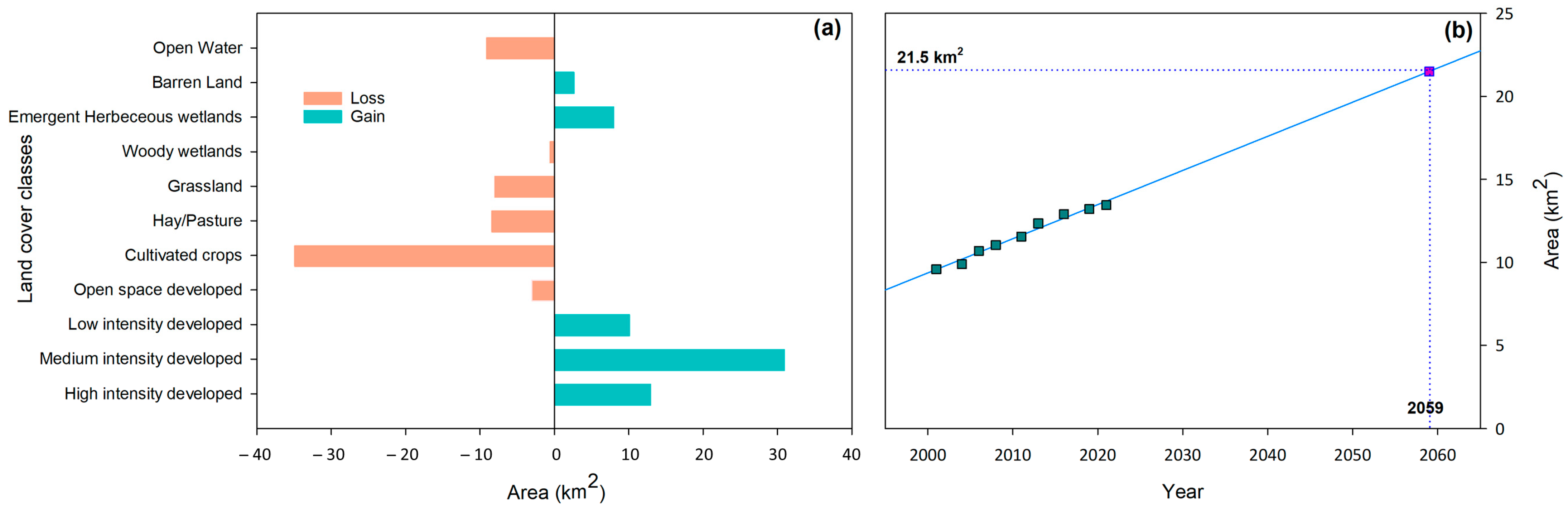
2.3. Climate Change and Urbanization

Two different scenarios, ‘Present’ and ‘Future’, were compared to assess the impacts of climate change and urbanization on hydrology, especially surface runoff. The ‘Present’ scenario corresponds to the period 2005–2014, while the ‘Future’ scenario reflects the period 2054–2063.

For our future projections of climate in the mid-21st century, Coupled Model Intercomparison Project Phase 5 (CMIP-5) projected climate data were downloaded from the Downscaled CMIP3 and CMIP5 Climate and Hydrology Projections (https://gdo-dcp.ucllnl.org/downscaled_cmip_projections/dcpInterface.html (accessed on 10 January 2024)). The BCCAv2-CMIP5-Climate-daily precipitation data from the RCP8.5 projections were employed. Data generated by csiro-mk3-6-0 were selected from the available 21 General Circulation Models (GCM) employing the 1/8-degree daily bias-correction and constructed analogs (BCCA) projections. Urbanization was predicted using the EVA tool (https://www.mrlc.gov/eva/ (accessed on 10 January 2024)) from the Multi-Resolution Land Characteristics (MRLC) Consortium data.

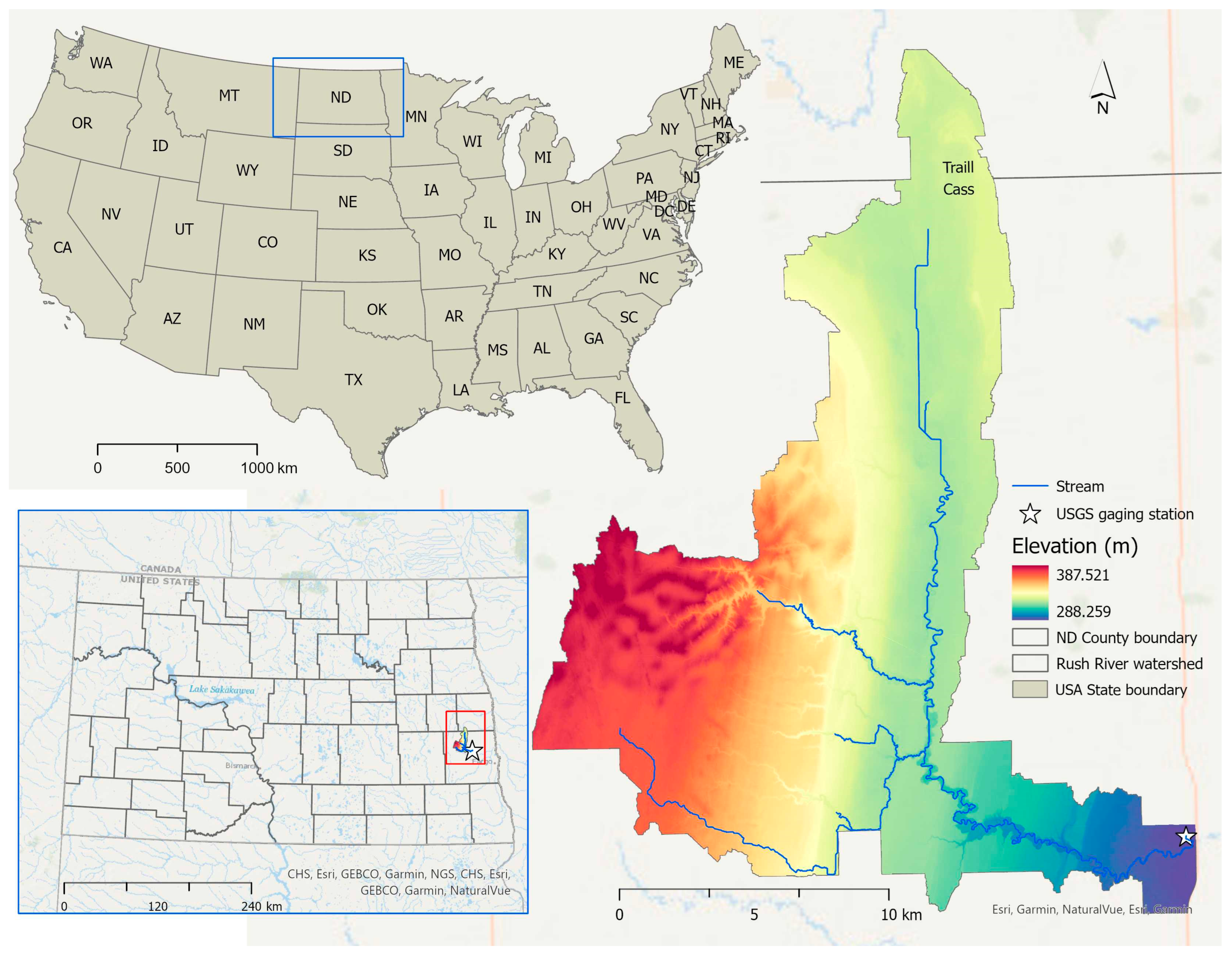
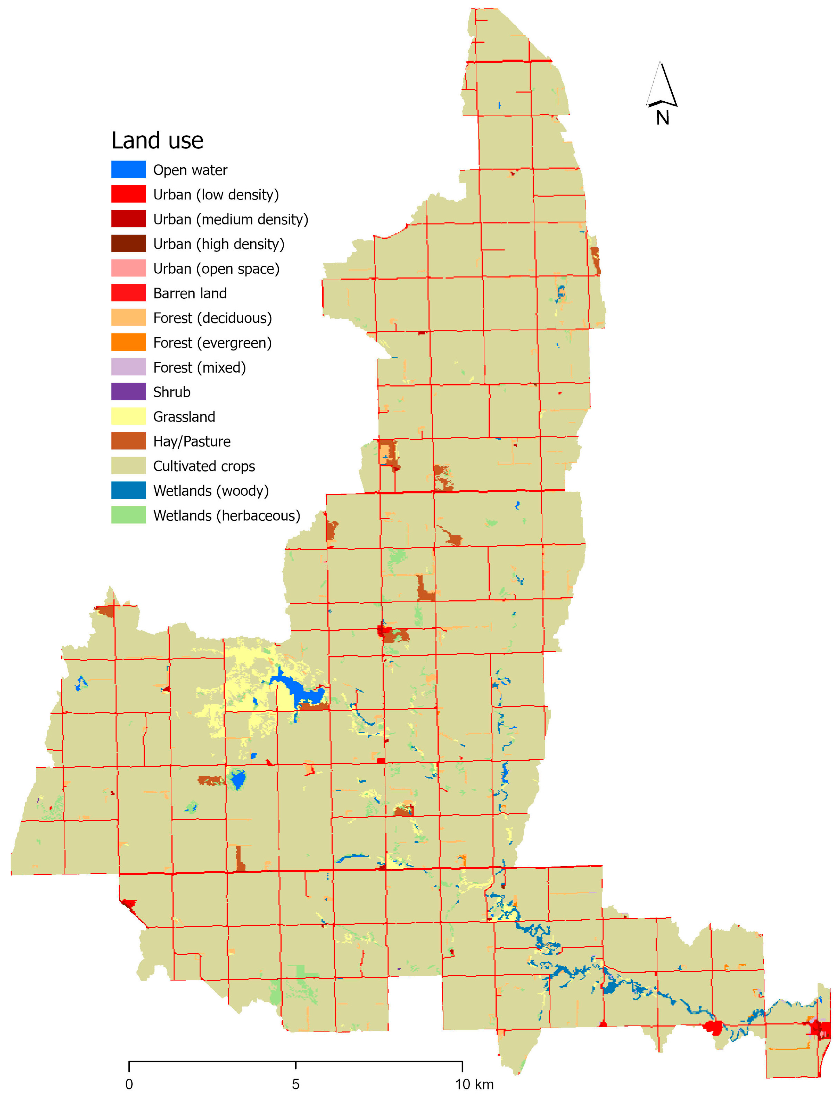
2.4. Study Area and Model Setup

The Rush River Watershed is in the southeastern region of North Dakota, USA (Figure 1). The watershed area is 297.92 km², and it is 330 m above sea level, on average. The highest elevation (i.e., 387 m) in the watershed is in the western portion, while the lowest elevation (i.e., 288 m) is in the southeastern portion. This agricultural watershed comprises 11 various soil types according to the Soil Survey Geographic (SSURGO) Database. The USGS 05060500 Rush River at the Amenia, ND gaging station (latitude 47°01′00″, longitude 97°12′50″) was considered as the watershed outlet.

A 10 m Digital Elevation Model (DEM) downloaded from the NRCS Geospatial data gateway was utilized for watershed delineation. In ArcSWAT, the default method for delineation was selected. After delineation, the whole watershed was divided into 11 sub-basins eventually. To perform HRU analysis, the Land Use and Land Cover (LULC) data were downloaded from the NRCS Geospatial data gateway. The soil types were obtained from the Soil Survey Geographic (SSURGO) Database. The terrain slopes were generated on the basis of the DEM in ArcSWAT. The selected thresholds for LULC, soil types, and slopes were 2%, 15%, and 15%, respectively. Eventually, 53 HRUs were defined. The temperature data (i.e., maximum and minimum temperatures) and precipitation data at daily time steps were downloaded from the Parameter-elevation Regressions on Independent Slopes Model (PRISM). In addition, other climate data including wind speed, solar radiation, and relative humidity, were downloaded from the Prediction Of Worldwide Energy Resources (POWER) Data Access Viewer.

The SWAT-CUP (Calibration Uncertainty Program) [30] was utilized for the calibration and validation of the enhanced SWAT model using the observed discharges at the selected USGS gaging station from the USGS National Water Information System. The SUFI-2 (Sequential Uncertainty Fitting, version 2) algorithm [31] in SWAT-CUP was employed for sensitivity and uncertainty analysis. During the simulation period, three years (i.e., 2002–2004) were selected for the warm-up. Five years (i.e., 2005–2009) were selected for the calibration. After the calibration period, the following 5-year period (i.e., 2010–2014) was selected for validation. To evaluate the performance of the enhanced SWAT model, three popular statistical metrics were selected: (1) Nash–Sutcliffe efficiency (NSE), (2) root mean square error (RMSE)–observations standard deviation ratio (RSR), and (3) coefficient of determination (R²) [32]. The NSE, RSR, and R², respectively, are given by:

$$\mathrm{N}\mathrm{S}\mathrm{E}=1-\frac{{\sum }_{\mathrm{i}=1}^{\mathrm{n}}{({\mathrm{O}}_{\mathrm{i}}-{\mathrm{S}}_{\mathrm{i}})}^2}{{\sum }_{\mathrm{i}=1}^{\mathrm{n}}{({\mathrm{O}}_{\mathrm{i}}-{\mathrm{O}}_{\mathrm{m}\mathrm{e}\mathrm{a}\mathrm{n}})}^2}$$

(8)

$$\mathrm{R}\mathrm{S}\mathrm{R}=\frac{\sqrt{{\sum }_{\mathrm{i}=1}^{\mathrm{n}}{({\mathrm{O}}_{\mathrm{i}}-{\mathrm{S}}_{\mathrm{i}})}^2}}{\sqrt{{\sum }_{\mathrm{i}=1}^{\mathrm{n}}{({\mathrm{O}}_{\mathrm{i}}-{\mathrm{O}}_{\mathrm{m}\mathrm{e}\mathrm{a}\mathrm{n}})}^2}}$$

(9)

$${\mathrm{R}}^2={[\frac{{\sum }_{\mathrm{i}=1}^{\mathrm{n}}({\mathrm{O}}_{\mathrm{i}}-{\mathrm{O}}_{\mathrm{m}\mathrm{e}\mathrm{a}\mathrm{n}})({\mathrm{S}}_{\mathrm{i}}-{\mathrm{S}}_{\mathrm{m}\mathrm{e}\mathrm{a}\mathrm{n}})}{\sqrt{{\sum }_{\mathrm{i}=1}^{\mathrm{n}}{({\mathrm{O}}_{\mathrm{i}}-{\mathrm{O}}_{\mathrm{m}\mathrm{e}\mathrm{a}\mathrm{n}})}^2}\sqrt{{\sum }_{\mathrm{i}=1}^{\mathrm{n}}{({\mathrm{S}}_{\mathrm{i}}-{\mathrm{S}}_{\mathrm{m}\mathrm{e}\mathrm{a}\mathrm{n}})}^2}}]}^2$$

(10)

where n is the total number of time steps; ${\mathrm{O}}_{\mathrm{i}}$ is the observed value at time step i; ${\mathrm{S}}_{\mathrm{i}}$ is simulated value at time step i; ${\mathrm{O}}_{\mathrm{m}\mathrm{e}\mathrm{a}\mathrm{n}}$ is the mean of the observed value; and ${\mathrm{S}}_{\mathrm{m}\mathrm{e}\mathrm{a}\mathrm{n}}$ is the mean of the simulated value.

2.5. Modeling Scenarios

The calibrated model (2005–2014) was selected as the present scenario. To set up the future baseline scenario, the predicted precipitation and urbanization during the period 2054–2063 were utilized. The precipitation data from CMIP-5 were incorporated into the input of the calibrated model and replaced the precipitation data from 2005 to 2014. Based on the predicted urbanization using the EVA tool, the curve numbers (CNs) during the period 2054–2063 were estimated and further utilized to replace the present ones in the calibrated model. Eventually, the future baseline scenario without any infiltration was built up.

To explore the functionality of the infiltration basin, more scenarios with infiltration basins were built based on the future baseline scenario. Qi et al. (2021) assessed the impacts of water head in infiltration basins on artificial recharge and assumed the water head range was from 0.1 to 1 m [7]. In this study, the depth of infiltration basins was assumed to be 1 m for a maximal water head of 1 m. The availability of the upstream surface runoff was not considered in this primary study. In this case, the proportion of the upstream surface runoff flowing into the infiltration basin was assumed to be a maximal value of 1. To consider the impacts of logging in the vadose zone during artificial recharge [28,29], the coefficient accounting for impacts of logging was assumed to be 0.1. The areas of infiltration basins were assumed to vary from 0.3% to 10% of the urban areas of the Rush River watershed. To assess the capability of infiltrations for artificial recharge, average annual discharge was selected as an indicator. To explore the capability for flood mitigation, peak portions of annual discharge were determined using a flow rate threshold of 5 m³/s.

3. Results and Discussion

3.1. Modeling Performance

Based on sensitivity analysis in SWAT-CUP, 12 parameters were selected for the calibration.

Table 1. Parameters for calibration of the enhanced SWAT model.

Parameter	Description	Calibrated Values
* CN2.mgt	SCS curve number for moisture condition II	vary
GWQMN.gw	Threshold depth of water in the shallow aquifer required for return flow to occur (mm H2O)	3336.553
GW_REVAP.gw	Groundwater “revap” coefficient	0.134851
REVAPMN.gw	Threshold depth of water in the shallow aquifer for “revap” to occur (mm H2O)	216.2931
ESCO.hru	Soil evaporation compensation factor	0.797276
SMTMP.bsn	Snow melts base temperature (°C)	−1.03802
SFTMP.bsn	Snowfall temperature	4.557257
SMFMX.bsn	Minimum melt rate for snow during the year (occurs on winter solstice)	7.933271
SMFMN.bsn	Maximum melt rate for snow during the year (occurs on the summer solstice)	4.719988
TIMP.bsn	Snowpack temperature lag factor	0.171148
CH_N2.rte	Manning’s roughness coefficient “n” value for the main channel	0.031751
CH_N1.sub	Manning’s “n” value for the tributary channels	0.065375

Note(s): * The relative method was applied for those parameters, and the replace method was applied for the rest of the parameters.

lists the 12 parameters and their description and calibrated values.

Observed and simulated hydrographs and precipitation during the entire simulation period are shown in Figure 2. The model performance was evaluated using three statistical metrics [32]. For the calibration period (i.e., 2005–2009), the NSE, RSR, and R² were calculated as 0.63, 0.61, and 0.63, respectively. For the validation period (i.e., 2010–2014), the NSE, RSR, and R² were 0.51, 0.7, and 0.53, respectively. The calculated statistical metrics demonstrated that the model performance was “satisfactory” [32]. Although the overall performance was satisfactory, some slight underestimations, especially for the early spring peaks (e.g., 2006, 2009, 2010, and 2011), were observed, as shown in Figure 2. This type of underestimation of the spring peaks due to snowmelt can be attributed to the limited capability of SWAT to simulate snowpack- and snowmelt-related hydrologic processes in cold regions. Similar findings were also demonstrated by Shabani et al. [33], Tahmasebi Nasab et al. [34], and Zeng et al. [35] in their SWAT modifications and applications to watersheds in cold regions.

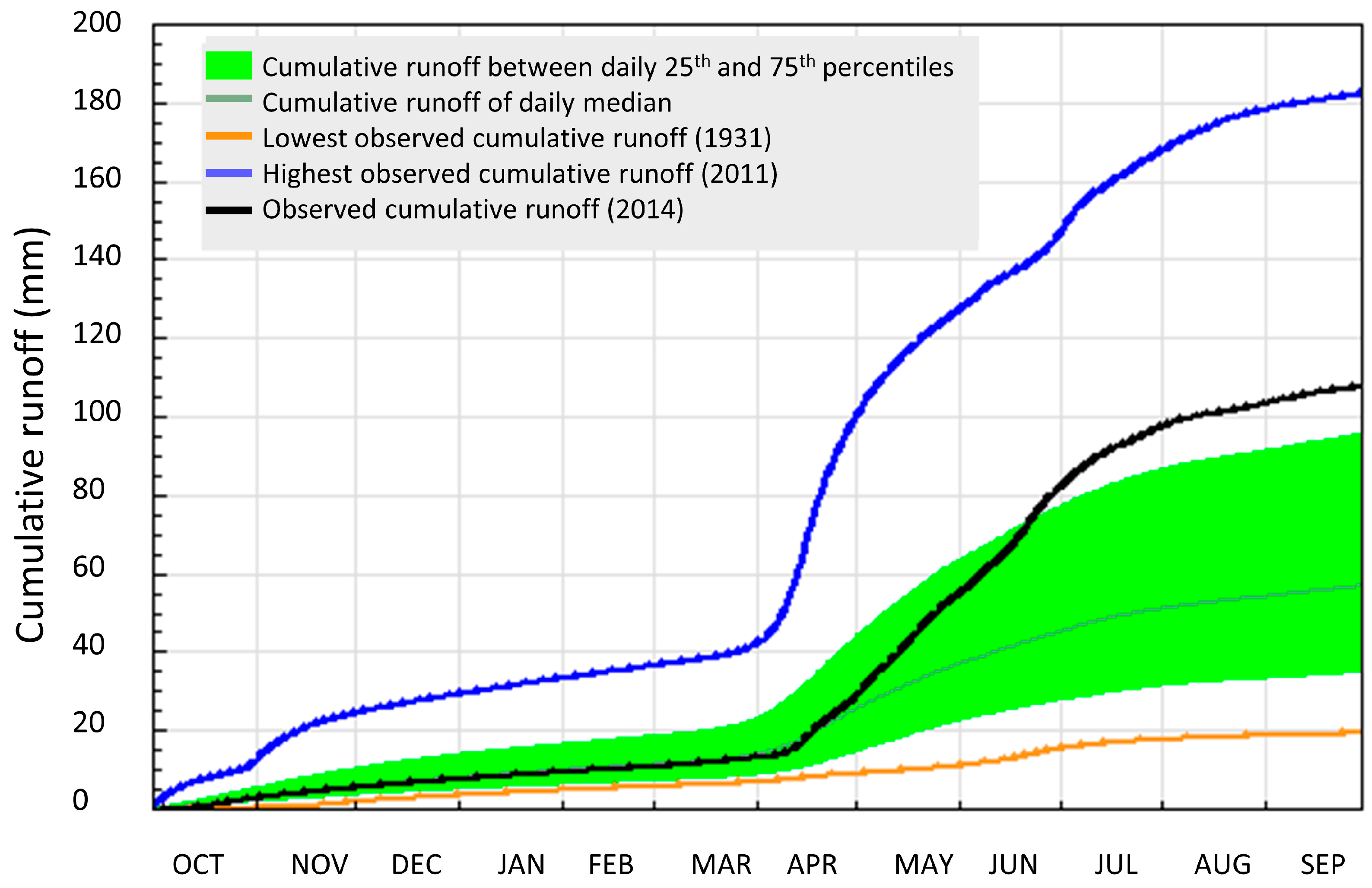
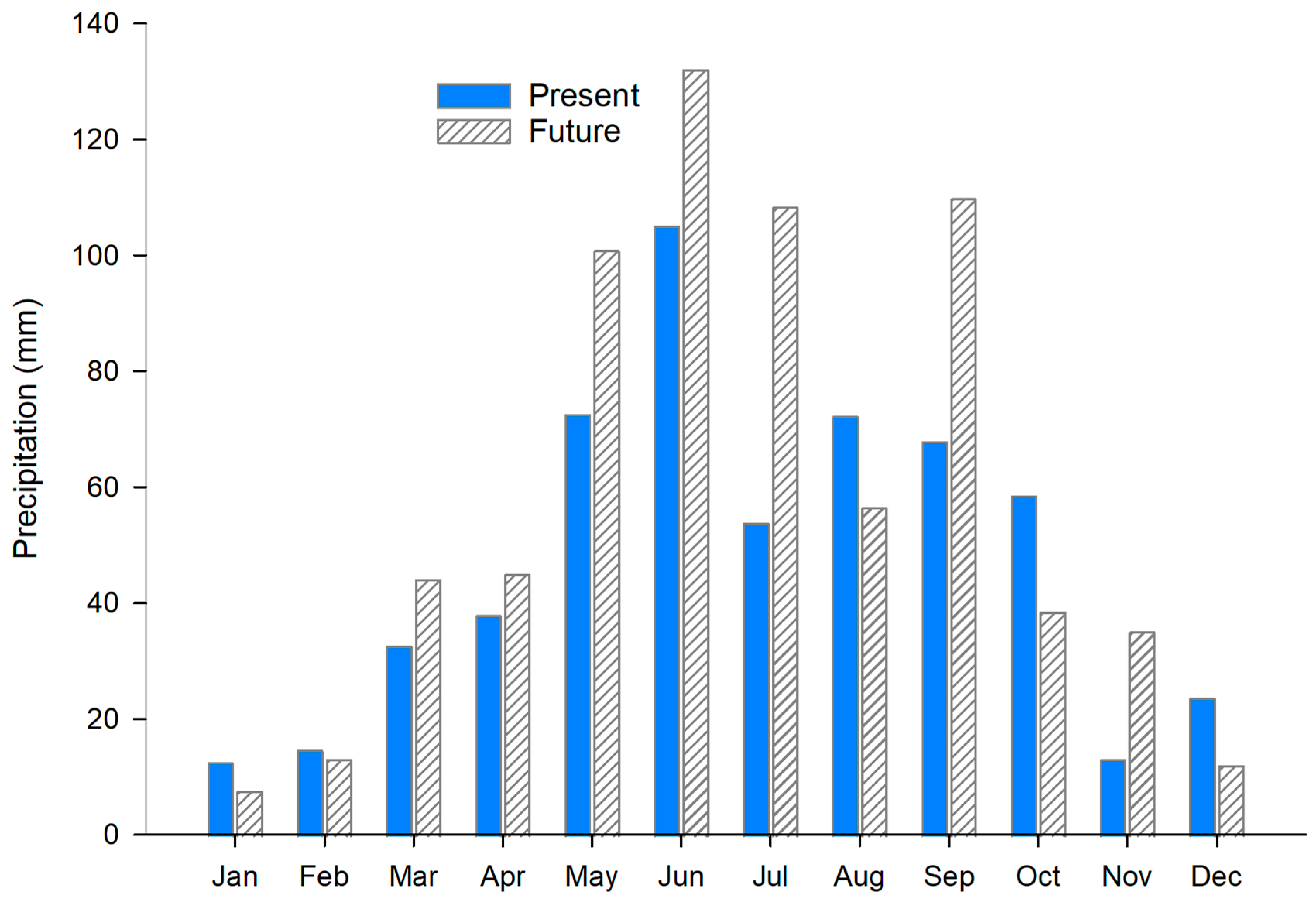
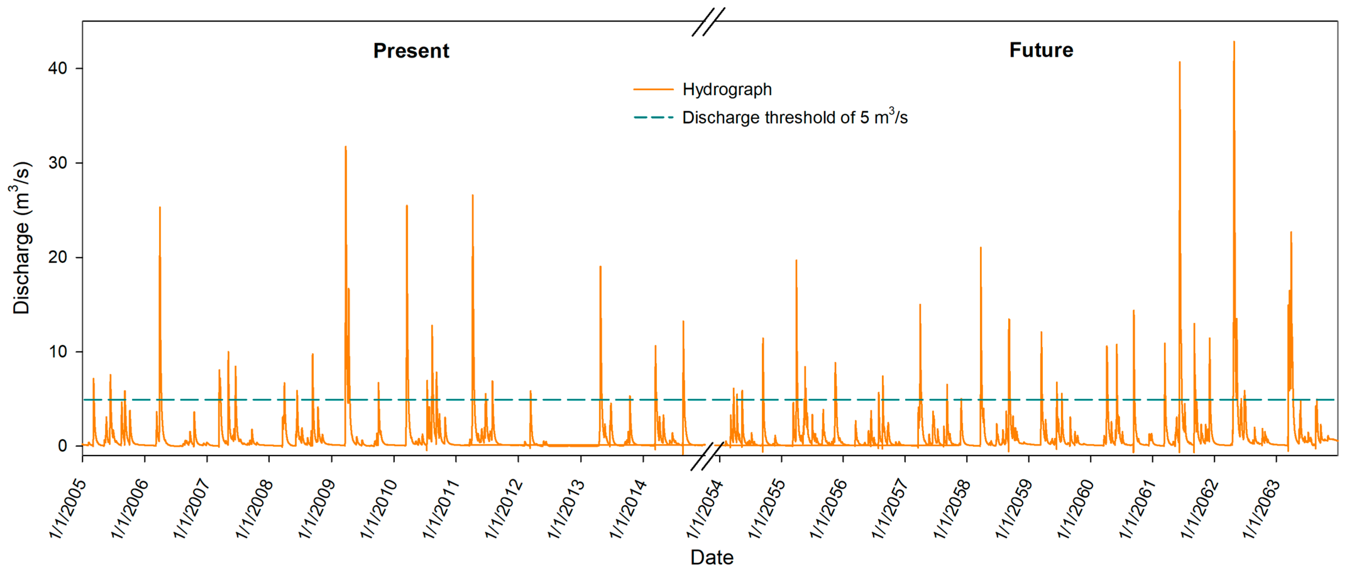
3.2. Changes in Precipitation, Urbanization, and Discharge

The Rush River watershed is a part of the Souris-Red-Rainy water resource region. The daily median cumulative runoff of the region varies from 1.47 to 9.26 mm in the winter and 31.66–55.75 mm in the spring and summer (data collected from the USGS WaterWatch at https://waterwatch.usgs.gov (accessed on 10 January 2024)). Analysis of long-term data from the USGS WaterWatch reveals significant seasonal variation in the Souris-Red-Rainy water resource region. The region observed its highest cumulative runoff of 180.90 mm in 2011 and its lowest cumulative runoff in 1931 (Figure 3). In 2014, the water resource region observed above-normal cumulative runoff in the summer, indicating potential shifts in hydrological patterns over time. Understanding these patterns of variability in cumulative runoff is essential for effective water resource management and planning in the Souris-Red-Rainy region, particularly within sub-watersheds like the Rush River watershed.

Compared with the present period, in the spring and summer seasons (March to July), average precipitation is projected to increase from 18.63% to 166.16% in future years (Figure 4). In contrast, precipitation is expected to decrease from 10.36% to 48.86% compared to the present time in the winter months. The present average annual precipitation of the study area is 565.90 mm, which will be increased to 703.99 mm in the Future scenario.

According to the National Land Cover Database 2011 (NLCD 2011), most of the land in the Rush River watershed is used for agriculture (89.9%), followed by urban use (4.3%) and range grass and hay fields (2.5%) (Figure 5). Using data from the EVA tool (https://www.mrlc.gov/eva/ (accessed on 10 January 2024)) of the Multi-Resolution Land Characteristics (MRLC) Consortium, the gain in medium-, high-, and low-intensity urban lands in this area was 84.2%, 72.1%, and 12.8%, respectively, during the period 2001 to 2021 (Figure 6a). The area had an urbanization growth rate of 40.5% in 2021 compared to 2001. Based on this rate, the total urban land area in the Rush River watershed is predicted to reach 21.5 km², compared to the current area of 13.4 km² (Figure 6b).

Because of the greater precipitation and larger urban area, the average annual discharge was predicted to reach 126.89 mm, compared to the present discharge of 98.81 mm (Figure 7). The peak portions were predicted to be 29.81 mm, compared to 21.44 mm in the present scenario, indicating that the peak portions were predicted to increase from 21.7% to 23.5%. Similar findings were noted by Khanaum and Borhan [36] in which peak discharge increased with an increase in impervious areas and rainfall depths.

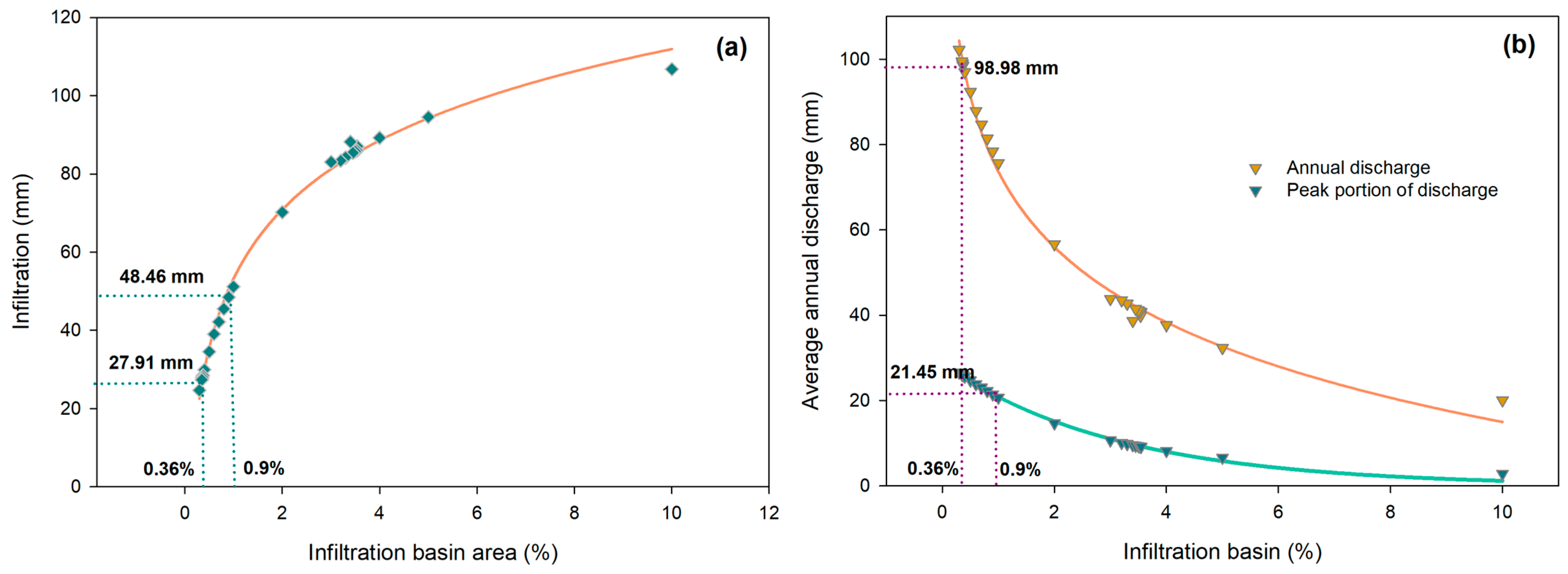
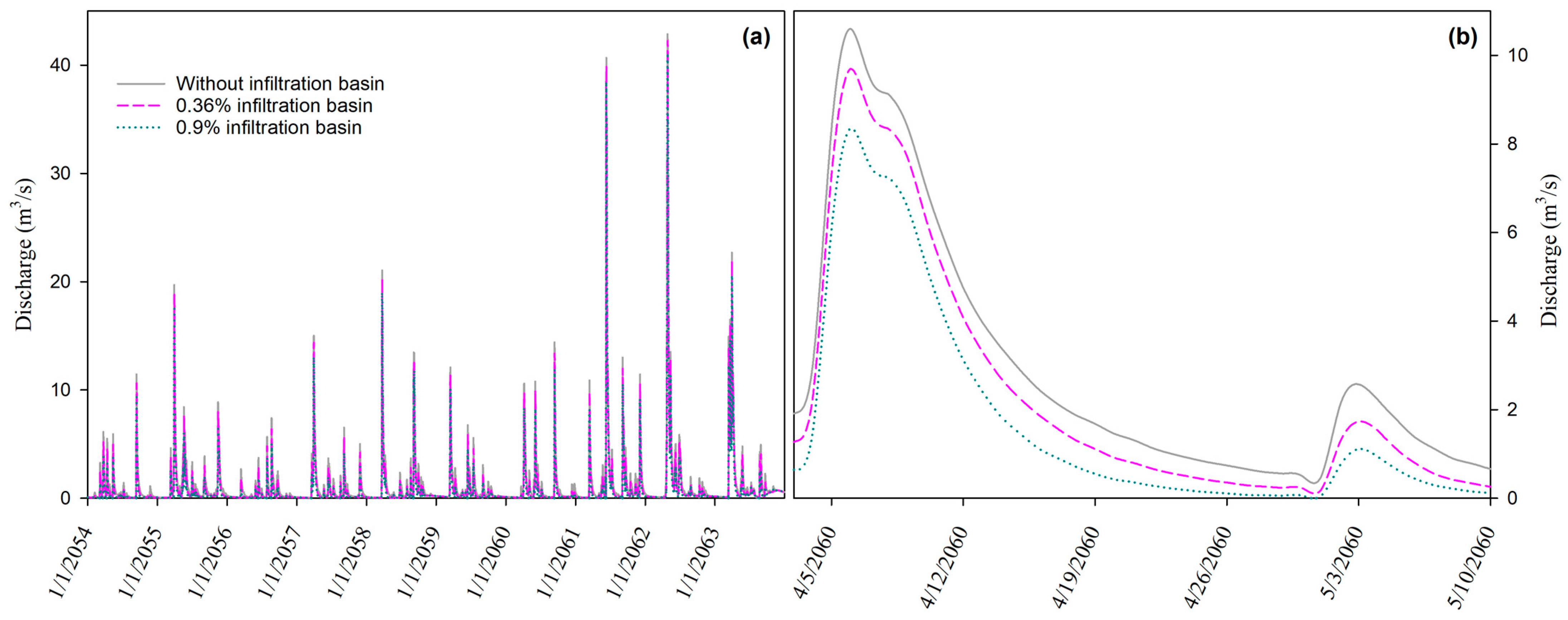
3.3. Impacts of Artificial Recharge via Infiltration Basin

With the increment in the area of infiltration basins, the annual infiltration was predicted to increase (Figure 8a), and the annual discharge was predicted to decrease (Figure 8b). A similar relationship between the radius of infiltration basins and infiltration was also observed by Qi et al. [7] in their simulation. With an infiltration basin area of 0.36%, the annual infiltration was predicted to be 27.91 mm (Figure 8a), and the annual discharge was predicted to be 98.98 mm (Figure 8b), similar to the annual discharge in the present scenario (i.e., 98.81 mm). In this case, the infiltration basin area of 0.36% in the urban area was enough to perform artificial recharge and offset the extra quantity of surface runoff in the future scenario. However, the peak portions were predicted to be 25.99 mm, which are greater than the peak portions in the present scenario (i.e., 21.44 mm), indicating that the infiltration basin area of 0.36% in the urban area was not enough to offset the extra flood events in the future scenario.

With an infiltration basin area of 0.9%, the annual infiltration was predicted to be 48.46 mm (Figure 8a), and the peak portions of the annual discharge were predicted to be 21.45 mm (Figure 8b), which are similar to the peak portions in the present scenario (i.e., 21.44 mm). In this case, the infiltration basin area of 0.9% in the urban area was enough to offset the extra flooding in the future scenario. However, the annual discharge was predicted to be 78.44 mm, which is smaller than the annual discharge in the present scenario (i.e., 98.81 mm), indicating that the infiltration basin area of 0.9% in the urban area would lead to insufficient surface runoff in the future scenario, especially for baseflow (Figure 9a,b. A single storm event was selected as an example of the impacts of the two different infiltration basin areas (Figure 9b). With an infiltration basin area of 0.9%, 21% of the peak flow would be mitigated, which is greater than an 8% mitigation of peak flow associated with an infiltration basin area of 0.36%. However, with an infiltration basin area of 0.9%, the minimum baseflow was predicted to reach only 0.05 m³/s, while the minimum baseflow was predicted to be 0.19 m³/s with an infiltration basin area of 0.36% (Figure 9b).

The smaller infiltration basin area (i.e., 0.36%) was enough to offset the extra quantity of surface runoff, while the lager infiltration basin area (i.e., 0.9%) was required for flood mitigation, especially for peak flows. However, the lager infiltration basin area would lead to insufficient baseflow. To mitigate peak flows and maintain baseflow, larger infiltration basins are recommended, while intermittent regulation of the infiltration basins according to different hydrologic periods is required. During flood periods, the infiltration basins should be fully operational, while during dry periods, the infiltration basins should be regulated to limit the collection of the surface runoff from the upstream flow based on the specific baseflow conditions.

4. Summary and Conclusions

A two-step modeling framework was performed to assess the offsets of artificial recharge via infiltration basins on the extra runoff induced by urbanization and extreme storms. Firstly, in the framework, a lumped infiltration basin module was developed and integrated into SWAT. Secondly, the precipitation and urbanization in the future scenario were projected and incorporated into the enhanced SWAT. In the lumped infiltration basin module, an area–storage relationship with one threshold for the shallow and wide shapes of infiltration basins was proposed. In addition, a coefficient was introduced to consider the impacts of logging in the vadose zone during artificial recharge.

The proposed modeling framework was applied to the Rush River Watershed in ND, USA. Various scenarios of infiltration basin areas were designed to explore their impacts on artificial recharge and flood mitigation. The results demonstrated the capability of the infiltration basins to influence both artificial recharge and flood mitigation. To mitigate floods, especially for peak flows, larger areas of infiltration basins are required compared to artificial recharge purposes only. Based on different demands, intermittent regulation of the infiltration basins according to different hydrologic periods is recommended. The offsets of artificial recharge on the extra surface runoff provide insight into the comprehensive preservation and management of surface water resources and groundwater resources.

References

1. Jasechko, S.; Seybold, H.; Perrone, D.; Fan, Y.; Shamsudduha, M.; Taylor, R.G.; Kirchner, J.W. Rapid groundwater decline and some cases of recovery in aquifers globally. Nature 2024, 625, 715–721. [Google Scholar]
2. Hernandez, E.A.; Uddameri, V. Standardized precipitation evaporation index (SPEI)-based drought assessment in semi-arid south Texas. Environ. Earth Sci. 2014, 71, 2491–2501. [Google Scholar] [CrossRef]
3. Dillon, P.; Stuyfzand, P.; Grischek, T.; Lluria, M.; Pyne, R.D.; Jain, R.C.; Bear, J.; Schwarz, J.; Wang, W.; Fernandez, E.; et al. Sixty years of global progress in managed aquifer recharge. Hydrogeol. J. 2018, 27, 1–30. [Google Scholar] [CrossRef]
4. Robinson, W.A. Climate change and extreme weather: A review focusing on the continental United States. J. Air Waste Manag. Assoc. 2021, 71, 1186–1209. [Google Scholar] [CrossRef]
5. Siddik, M.S.; Tulip, S.S.; Rahman, A.; Islam, M.N.; Haghighi, A.T.; Mustafa, S.M.T. The impact of land use and land cover change on groundwater recharge in northwestern Bangladesh. J. Environ. Manag. 2022, 315, 115130. [Google Scholar] [CrossRef]
6. Rahman, A.; Mojid, M.A.; Banu, S. Climate change impact assessment on three major crops in the north-central region of Bangladesh using DSSAT. Int. J. Agric. Biol. Eng. 2018, 11, 135–143. [Google Scholar] [CrossRef]
7. Qi, T.; Shu, L.; Li, H.; Wang, X.; Men, Y.; Opoku, P.A. Water distribution from artificial recharge via infiltration basin under constant head conditions. Water 2021, 13, 1052. [Google Scholar] [CrossRef]
8. Wu, P.; Comte, J.C.; Li, F.; Chen, H. Influence of tides on the effectiveness of artificial freshwater injection in mitigating seawater intrusion in an unconfined coastal aquifer. J. Hydrol. 2023, 617, 129043. [Google Scholar] [CrossRef]
9. Wu, P.; Shu, L.; Comte, J.C.; Zuo, Q.; Wang, M.; Li, F.; Chen, H. The effect of typical geological heterogeneities on the performance of managed aquifer recharge: Physical experiments and numerical simulations. Hydrogeol. J. 2021, 29, 2107–2125. [Google Scholar] [CrossRef]
10. Stefan, C.; Ansems, N. Web-based global inventory of managed aquifer recharge applications. Sustain. Water Resour. Manag. 2018, 4, 153–162. [Google Scholar] [CrossRef]
11. Ringleb, J.; Sallwey, J.; Stefan, C. Assessment of Managed Aquifer Recharge through Modeling—A Review. Water 2016, 8, 579. [Google Scholar] [CrossRef]
12. Khan, S.; Mushtaq, S.; Hanjra, M.A.; Schaeffer, J. Estimating potential costs and gains from an aquifer storage and recovery program in Australia. Agric. Water Manag. 2008, 95, 477–488. [Google Scholar] [CrossRef]
13. Steinel, A.; Schelkes, K.; Subah, A.; Himmelsbach, T. Spatial multi-criteria analysis for selecting potential sites for aquifer recharge via harvesting and infiltration of surface runoff in north Jordan. Hydrogeol. J. 2016, 24, 1753–1774. [Google Scholar] [CrossRef]
14. Beganskas, S.; Fisher, A.T. Coupling distributed stormwater collection and managed aquifer recharge: Field application and implications. J. Environ. Manag. 2017, 200, 366–379. [Google Scholar] [CrossRef]
15. Fatkhutdinov, A.; Stefan, C. Multi-Objective Optimization of Managed Aquifer Recharge. Groundwater 2018, 57, 238–244. [Google Scholar] [CrossRef]
16. Franczyk, J.; Chang, H. The effects of climate change and urbanization on the runoff of the Rock Creek basin in the Portland metropolitan area, Oregon, USA. Hydrol. Process. Int. J. 2009, 23, 805–815. [Google Scholar] [CrossRef]
17. Pan, S.; Liu, D.; Wang, Z.; Zhao, Q.; Zou, H.; Hou, Y.; Liu, P.; Xiong, L. Runoff responses to climate and land use/cover changes under future scenarios. Water 2017, 9, 475. [Google Scholar] [CrossRef]
18. Han, Q.; Xue, L.; Qi, T.; Liu, Y.; Yang, M.; Chu, X.; Liu, S. Assessing the Impacts of Future Climate and Land-Use Changes on Streamflow under Multiple Scenarios: A Case Study of the Upper Reaches of the Tarim River in Northwest China. Water 2023, 16, 100. [Google Scholar] [CrossRef]
19. Ebrahimian, A.; Gulliver, J.S.; Wilson, B.N. Effective impervious area for runoff in urban watersheds. Hydrol. Process. 2016, 30, 3717–3729. [Google Scholar] [CrossRef]
20. Bucton, B.G.B.; Shrestha, S.; Saurav, K.C.; Mohanasundaram, S.; Virdis, S.G.; Chaowiwat, W. Impacts of climate and land use change on groundwater recharge under shared socioeconomic pathways: A case of Siem Reap, Cambodia. Environ. Res. 2022, 211, 113070. [Google Scholar] [CrossRef] [PubMed]
21. Wang, R.; Kalin, L. Combined and synergistic effects of climate change and urbanization on water quality in the Wolf Bay watershed, southern Alabama. J. Environ. Sci. 2018, 64, 107–121. [Google Scholar] [CrossRef] [PubMed]
22. Mahdian, M.; Hosseinzadeh, M.; Siadatmousavi, S.M.; Chalipa, Z.; Delavar, M.; Guo, M.; Abolfathi, S.; Noori, R. Modelling impacts of climate change and anthropogenic activities on inflows and sediment loads of wetlands: Case study of the Anzali wetland. Sci. Rep. 2023, 13, 5399. [Google Scholar] [CrossRef] [PubMed]
23. Gassman, P.W.; Sadeghi, A.M.; Srinivasan, R. Applications of the SWAT model special section: Overview and insights. J. Environ. Qual. 2014, 43, 1–8. [Google Scholar] [CrossRef] [PubMed]
24. Jeong, J.; Kannan, N.; Arnold, J.; Glick, R.; Gosselink, L.; Srinivasan, R. Development and integration of sub-hourly rainfall–runoff modeling capability within a watershed model. Water Resour. Manag. 2010, 24, 4505–4527. [Google Scholar] [CrossRef]
25. Arnold, J.G.; Moriasi, D.N.; Gassman, P.W.; Abbaspour, K.C.; White, M.J.; Srinivasan, R.; Jha, M.K. SWAT: Model use, calibration, and validation. Trans. ASABE 2012, 55, 1491–1508. [Google Scholar] [CrossRef]
26. Neitsch, S.L.; Arnold, J.G.; Kiniry, J.R.; Williams, J.R. Soil and Water Assessment Tool Theoretical Documentation Version 2009; Texas Water Resources Institute: College Station, TX, USA, 2011.
27. Teatini, P.; Comerlati, A.; Carvalho, T.; Gütz, A.Z.; Affatato, A.; Baradello, L.; Paiero, G. Artificial recharge of the phreatic aquifer in the upper Friuli plain, Italy, by a large infiltration basin. Environ. Earth Sci. 2015, 73, 2579–2593. [Google Scholar] [CrossRef]
28. Schuh, W.M. Seasonal variation of clogging of an artificial recharge basin in a northern climate. J. Hydrol. 1990, 121, 193–215. [Google Scholar] [CrossRef]
29. Zou, Z.; Shu, L.; Min, X.; Chifuniro Mabedi, E. Clogging of infiltration basin and its impact on suspended particles transport in unconfined sand aquifer: Insights from a laboratory study. Water 2019, 11, 1083. [Google Scholar] [CrossRef]
30. Rouholahnejad, E.; Abbaspour, K.C.; Vejdani, M.; Srinivasan, R.; Schulin, R.; Lehmann, A. A parallelization framework for calibration of hydrological models. Environ. Model. Softw. 2012, 31, 28–36. [Google Scholar] [CrossRef]
31. Nash, J.E.; Sutcliffe, J.V. River flow forecasting through conceptual models part I—A discussion of principles. J. Hydrol. 1970, 10, 282–290. [Google Scholar] [CrossRef]
32. Moriasi, D.N.; Arnold, J.G.; Van Liew, M.W.; Bingner, R.L.; Harmel, R.D.; Veith, T.L. Model evaluation guidelines for systematic quantification of accuracy in watershed simulations. Trans. ASABE 2007, 50, 885–900. [Google Scholar] [CrossRef]
33. Shabani, A.; Zhang, X.; Chu, X.; Dodd, T.P.; Zheng, H. Mitigating Impact of Devils Lake Flooding on the Sheyenne River Sulfate Concentration. J. Am. Water Resour. Assoc. 2020, 56, 297–309. [Google Scholar] [CrossRef]
34. Tahmasebi Nasab, M.; Grimm, K.; Bazrkar, M.H.; Zeng, L.; Shabani, A.; Zhang, X.; Chu, X. SWAT modeling of non-point source pollution in depression-dominated basins under varying hydroclimatic conditions. Int. J. Environ. Res. Public Health 2018, 15, 2492. [Google Scholar] [CrossRef] [PubMed]
35. Zeng, L.; Shao, J.; Chu, X. Improved hydrologic modeling for depression-dominated areas. J. Hydrol. 2020, 590, 125269. [Google Scholar] [CrossRef]
36. Khanaum, M.M.; Borhan, M.S. Effects of Increasing Rainfall Depths and Impervious Areas on the Hydrologic Responses. Open J. Mod. Hydrol. 2023, 13, 114–128. [Google Scholar] [CrossRef]
Figure 1. Location, boundary, and outlet of the Rush River watershed.
Water 16 01032 g001
Figure 2. Observed and simulated hydrographs and precipitation during the simulation period.
Water 16 01032 g002
Figure 3. Cumulative runoff hydrograph for the Souris-Red-Rainy water resource region (figure adopted from the USGS WaterWatch).
Water 16 01032 g003
Figure 4. Comparison of precipitation in the Rush River watershed for Present and Future scenarios.
Water 16 01032 g004
Figure 5. Current land use and land cover of the Rush River watershed.
Water 16 01032 g005
Figure 6. (a) Changes in land cover classes from 2001 to 2021; (b) projection of urban land area in the Rush River watershed for the year 2059.
Water 16 01032 g006
Figure 7. Simulated hydrographs in the Rush River watershed for Present and Future scenarios.
Water 16 01032 g007
Figure 8. (a) Annual infiltrations under different portions of the infiltration basin areas in the urban area; (b) annual discharges under different portions of the infiltration basin areas in the urban area.
Water 16 01032 g008
Figure 9. Daily discharges under different portions of the infiltration basin areas in the urban area; (a) future period and (b) a single storm event.
Water 16 01032 g009