Article

The Impact of Climate Change on Hydro-Meteorological Droughts in the Chao Phraya River Basin, Thailand

1
Department of Meteorology and Hydrology, Faculty of Water Resources, National University of Laos, Vientiane 01020, Laos
2
Department of Water Resources Engineering, Faculty of Engineering, Chulalongkorn University, Bangkok 10330, Thailand
3
Disaster and Risk Management Information Systems Research Unit, Chulalongkorn University, Bangkok 10330, Thailand
4
Water Resources Engineering Division, Civil Engineering Department, Faculty of Engineering, King Mongkut’s University of Technology Thonburi, Bangkok 10140, Thailand
*
Author to whom correspondence should be addressed.
Water 2024, 16(7), 1023; https://doi.org/10.3390/w16071023
Submission received: 28 February 2024 / Revised: 24 March 2024 / Accepted: 25 March 2024 / Published: 1 April 2024

Abstract

:
This study evaluated the impacts of climate change on hydro-meteorological droughts in the Chao Phraya River Basin (CPRB), Thailand under two Representative Concentration Pathway (RCP) scenarios (RCP4.5 and RCP8.5). We used three Reginal Climate Models (RCMs) of the Southeast Asia Regional Climate Downscaling/Coordinated Regional Climate Downscaling Experiment—Southeast Asia (SEACLID/CORDEX-SEA), which are bias corrected. The Soil and Water Assessment Tool (SWAT) was used to simulate streamflow for future periods. The Standardized Precipitation Index (SPI) and Standardized Streamflow Index (SSI) were estimated and used for drought characterization at three time scales (3, 6, and 12 months). The lag time between meteorological and hydrological droughts is approximately 1–3 months. The results suggest that the CPRB is likely to experience less frequent hydro-meteorological drought events in the future. The meteorological drought is projected to be longer, more severe, and intense. The severity of hydrological drought tends to decrease, but the intensity could increase. Climate change has been discovered to alter drought behaviors in the CPRB, posing a threat to drought monitoring and warning because droughts will be less predictable in future climate scenarios. The characterization of historical and future droughts over the CPRB is therefore valuable in developing an improved understanding of the risks of drought.

1. Introduction

Droughts are a type of major natural disaster that occur in many parts of the world. They are different from other natural disasters in many aspects. Most frequently occurring disasters, such as floods and storms [1], are rapid-onset hydrologic events taking place in specific and limited areas and causing immediate damage and losses. A drought is a slow-developing, gradual natural hazard that can occur anywhere in the world. The identification of the onset and termination of a drought is difficult. Droughts can have a serious impact on health, agriculture, economies, and the environment [2]. The impacts of droughts are widespread, non-structural, and less observable because the impacts often accumulate slowly over an extended period. It therefore remains a challenge to measure and fully account for the impact of a drought [3,4,5,6]. Droughts have been recognized as the most complex and most destructive natural disasters in terms of their impacts on a higher number of people compared to other forms of hazards [7,8]. According to the Food and Agriculture Organization (FAO), droughts are the world’s costliest natural disasters, accounting for USD 6–8 billion annually, and impacting more people than any other form of natural disaster.
According to the Special Report on Extremes (SREX) published by the Intergovernmental Panel on Climate Change (IPCC) in 2021, some regions have experienced increasing lengths and intensities of flood and/or drought events. It is important to develop an increased understanding of historical droughts to prepare for future drought conditions. As droughts will continue to be a crucial problem in the world, much effort is needed to better understand and mitigate their effects. To describe drought characteristics, such as their frequency, intensity, and duration, drought indices, based on climatic and hydrological variables, are often used. Unlike the time series of a single variable, drought indices consider a range of variables that can influence drought conditions, such as precipitation, soil moisture, and evapotranspiration, and they provide a more comprehensive overview of the state of drought in an area. Using drought indices can offer a better understanding of the complex factors that contribute to droughts. Drought indices are useful tools for drought monitoring and prediction, which provide necessary information to make decisions related to water management and resource allocation, as well as for planning and preparedness efforts in the event of a drought.
Thailand is one of the most drought-prone countries in the Asia–Pacific region [9]. Thailand has experienced droughts almost every year [10]. The probability of a drought event in Thailand for any given year is 45% [11]. According to the Department of Disaster Prevention and Mitigation (DDPM), 2013, 2014, 2015, 2016, and 2019 were severe drought years in the recent decade. In terms of water management, the drought in 2015 was the worst in the past 50 years. On 1 November 2015, the quantity of usable water for the upcoming dry season in the three major storage dams in the CPRB (see Figure 1) was at a critical level. The usable water reserve in the Bhumibol Dam was recorded at 1184 MCM (Million Cubic Meters), which was the lowest in the past 53 years. The Sirikit Dam had a reserve of 2056 MCM, which was the lowest in 20 years. The reserved water in Pasak dam was 637 MCM, which was the lowest in 17 years since its inception [10]. While there have been several drought studies in Thailand, most of these studies often examined historical drought conditions over the northeastern regions, e.g., [9,12,13,14,15,16,17]. Studies of drought characteristics and their changes due to climate change impacts in the CPRB are limited.
This study aims to develop an improved understanding of drought characteristics for the CPRB in Thailand, which is considered the most important basin in Thailand for several reasons such as economic development, agricultural production, and cultural and historical significance. The specific objectives are (1) to assess the accuracy of multiple RCMs in simulating streamflow over the CPRB and (2) to investigate the potential impacts of climate change on hydro-meteorological droughts using the standardized hydro-meteorological drought indices. The findings from this study can be used to evaluate the drought situations in other parts of Thailand or comparable climate regions to improve drought monitoring and warning.

2. Study Area

The Chao Phraya River Basin (CPRB), shown in Figure 1, was selected as the study area. It is located approximately between 13°30′ N to 19°50′ N latitude and 98°10′ E to 101°30′ E longitude. The approximate basin area of the CPRB is 158,507 km2, accounting for about 30% of the total country’s area. The elevation of the basin ranges from 0 to 3019 m above the mean sea level. The upper basin consists of alternating parallel ranges lying north–south and valleys forming the basins and headwaters of the four major tributaries of the Chao Phraya River—the Ping, Wang, Yom, and Nan rivers that drain southward. Located at the upper Ping and Nan rivers are the Bhumibol and Sirikit dams, respectively. The Pasak dam is built across the Pasak River in the southeast of the CPRB. The Chao Phraya dam at the central part of the CPRB is a diversion dam regulating the flow to the central plain, which stretches from the northern ranges and valleys down to the Gulf of Thailand. The Tha Chin River is a distributary that splits west from the Chao Phraya River in Chai Nat Province and flows directly to the sea. The Pasak River collects water from the east basin and joins the Chao Phraya River in Ayutthaya Province. The lower CPRB contains alluvial plains that are productive for agriculture. The analysis of the land use data from the Land Development Department (LDD), Thailand shows that about 45% of the CPRB comprises agricultural areas but only 12% of them are in an irrigation zone. Most agriculture in the CPRB is highly vulnerable to droughts because it relies heavily on rainfall. Agricultural produce is severely affected when there is low rainfall during September and October or when there is a long dry spell in June or July.
Thailand has distinct wet and dry climates. The main driver of seasonal rainfall variability is monsoon winds [18,19]. Based on the data in Table 1, which were obtained from the Thai Meteorological Department (TMD), the average annual rainfall in the CPRB is 1143 mm. A slight increasing rainfall gradient is found from the south to the north. Heavy rainfall is common during the rainy season from mid-May to mid-October when the Southwest monsoon brings warm moist air from the Indian Ocean. The dry season from mid-October to mid-February is caused by the northeast monsoon that flows from the cooler South China Sea. The period from mid-February to mid-May is the transitional period between monsoons, and this is when the weather becomes warmer. The average annual streamflow in the CPRB calculated from the data of the Royal Irrigation Department (RID), Thailand, as listed in Table 1, is approximately 1732 MCM. About 96% of the average annual streamflow is from the rainy season, and the rest is from the dry season. Droughts in Thailand are often caused by a lack of rainfall or less rainfall in the wet season and a long absence of rainfall in the dry season.

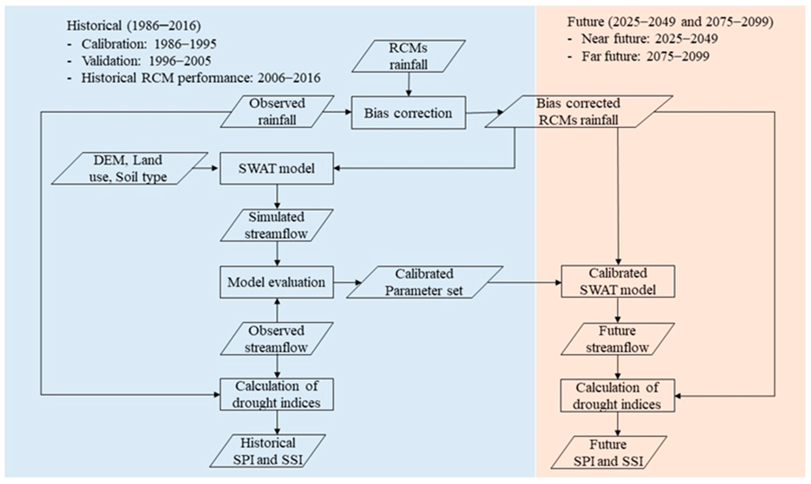
3. Materials and Methods

This study used the daily rainfall data from 68 gauges of the Thai Meteorological Department (TMD) between the years of 1986 and 2016. The daily streamflow data of 5 gauges in the Ping (P.1), Wang (W.1A), Yom (Y.1A), Nan (N.1), and Chao Phraya (C.2) Rivers from the 1986–2016 period were provided by the Royal Irrigation Department (RID). The locations of the gauges are shown in Figure 1. A schematic diagram of the overall framework is shown in Figure 2. Historical and future periods were defined to assess the impact of climate change on droughts. The observed rainfall and streamflow data were used for calibration and validation of Soil & Water Assessment Tool (SWAT) model and calculation of baseline drought indices. After bias correction, the ability of the Regional Climate Models (RCMs) in generating streamflow in a historical period was evaluated. The output from all selected RCMs was investigated with particular emphasis on the results of drought indices obtained from the best performing RCM. Additional results of drought indices obtained from less performing RCMs are provided in Appendix A and Appendix B. Details regarding SWAT modeling, RCM, and drought indices are provided in the following sections.

3.1. SWAT Modeling

The SWAT is a physically semi-distributed, continuous time hydrologic model [20,21] developed by the Agricultural Research Service (ARS) of the United States Department of Agriculture (USDA), Texas A&M University, and several federal agencies [22,23]. SWAT is one of the most widely used models in the world and has proven to be effective in simulating hydrology and hydro-meteorological extremes in river basins of varying scales around the world, particularly in Southeast Asia [24,25], where the quality of hydro-climatic data remains problematic [5,26]. It has demonstrated the potential to provide valuable insights into the impacts of land use, land management practices, and extreme climatic conditions.
SWAT simulates hydrological processes by dividing the spatial characteristics of the basin into subbasins and hydrological response units (HRUs) based on the unique combination of soil, land use, and slope features. The water balance equation, which is fundamental to SWAT simulation, is solved for each HRU. The simulation of the basin’s hydrology is separated into two phases. The land phase controls the amount of water that is available to flow into the main channel. The routing phase involves the movement of water through the channel network and ultimately to the outlet. A full description of the SWAT model can be found in [22].
Based on the review of SWAT studies in Southeast Asia presented in [27], about 50% of a total of 126 articles identified from 1998 to 2018 were conducted in Thailand and Vietnam. The main SWAT applications in the regions covered the model capability assessment, land use, and climate change assessment. The applications for simulating extreme events are particularly limited; thus, this area of research requires more attention. The SWAT model was applied in this study to simulate the streamflow for the near future (2025–2049) and far future (2075–2099) time periods. Calibration and validation of the SWAT model were conducted in the 1986–1995 and 1996–2005 periods accordingly using the SWAT-CUP tool [28] and manual adjustment. The performance of the calibrated model in simulating historical and future streamflow was evaluated using statistical parameters, including coefficient of determination (R2), Nash–Sutcliffe efficiency (NSE), and root mean square error (RMSE). The SWAT model performance ratings for a monthly time step simulation were classified as “very good”, “good”, “satisfactory”, and “unsatisfactory” when the NSE values ranged from 0.75 to 1, from 0.65 to 0.75, and from 0.50 to 0.65 and when they were <0.5, respectively. NSE values greater than 0.5 were considered acceptable [29,30]. The performance ratings for the daily time step simulation are relaxed with poorer values of performance statistics [31].

3.2. Regional Climate Model (RCM)

Based on the glossary of the American Meteorological Society (AMS), a regional climate model (RCM) is defined as “a numerical climate prediction model forced by specified lateral and ocean conditions from a general circulation model (GCM) or observation-based dataset (reanalysis) that simulates atmospheric and land surface processes, while accounting for high-resolution topographical data, land-sea contrasts, surface characteristics, and other components of the Earth-system”.
The RCM was developed to bridge the gap between the global but coarse estimates of the GCM, which typically had a spatial resolution of 100–300 km [32], and studies of regional phenomena with finer spatial resolutions [33], which are currently approximately 50 km to 12 km [34]. Driven by lateral boundary conditions and reanalysis data, RCMs can account for local-scale forcings and processes that are governed by complex topography, coastlines, inland bodies of water, and land cover distribution [35]. With an improved spatial resolution, RCMs can reproduce more accurate climate information than GCMs [36]. RCMs have widely been used to study regional climate variability, climate extremes, and the impacts of climate change [37,38,39,40]. A large number of RCMs are available from laboratories worldwide, and the number of new RCMs has been continuously increasing [35].
RCMs from the Southeast Asia Regional Climate Downscaling/Coordinated Regional Climate Downscaling Experiment—Southeast Asia (SEACLID/CORDEX-SEA) were used in several climate change studies in Southeast Asia. Recent peer-reviewed publications and more details of the CORDEX-SEA can be found in, e.g., [32,41,42,43,44,45].
Despite this advancement, there remains a need for further improvements regarding the uncertainty associated with climate projections. This is particularly the case of tropical climate regions where large discrepancies between historical simulation and future projections of precipitation are well known among the CMIP5 GCMs [46,47] and RCMs [48]. Several studies have used multi-model ensemble approaches to reduce intra- and inter-model uncertainty [48,49,50,51,52]. While ensemble projection can provide valuable information about the degree of uncertainties and risks associated with different RCMs, it also introduces ambiguity into decision-making processes because it presents a range of possible outcomes rather than a single, deterministic result. This can complicate the decision-making process [51,53,54].
In this study, the precipitation data from three RCMs including MPI, IPSL, and ICHEC under the two Representative Concentration Pathway (RCP) scenarios of RCP4.5 and RCP8.5 were obtained from the SEACLID/CORDEX-SEA, bias corrected with the widely used quantile mapping method [55], and used as input to the calibrated SWAT model. To avoid subjectivity in the interpretation of the RCM’s performance, the best performing RCM was identified based on statistical performance values and was used further, primarily for the representation of the future drought assessment. The RCMs and dataset used for the SWAT simulation are summarized Table 1.

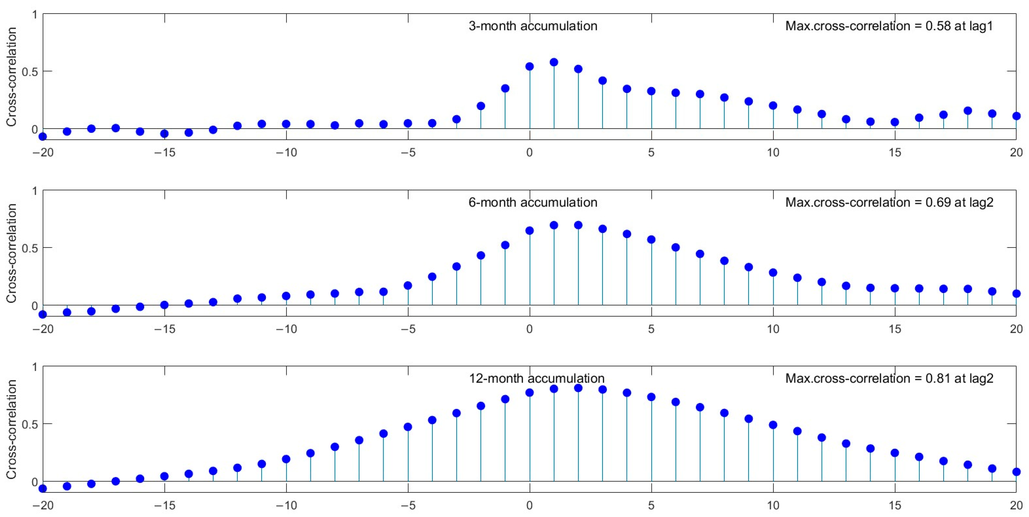
3.3. Drought Indices and Drought Characteristics

Droughts can be classified into four types based on the sequence of occurrence [56]. Meteorological droughts caused by precipitation deficit and dry weather are the first to occur prior to other types of droughts. When there is a prolonged period of dryness with little or no rainfall, it can lead to a decrease in soil moisture and agricultural drought, which affects the growth and production of crops. The evolution of an agricultural to hydrological drought is when there is a deficiency in the availability of water resources, such as surface water, groundwater, and water stored in reservoirs. If a hydrological drought continues for an extended period, it can have adverse socio-economic impacts, such as increased food prices, a loss of jobs, and reduced economic growth. A socio-economic drought can have severe consequences on the livelihoods of people living in affected regions. It is noted that not all droughts follow this exact progression and that the severity and duration of a drought can vary depending on the region and its specific climate conditions. Additionally, the impacts of drought can be influenced by human factors, such as land use change and water management practices [57].
Many studies have used standardized drought indices, such as Standardized Precipitation Index (SPI), Standardized Streamflow Index (SSI), and Standardized Precipitation Evapotranspiration Index (SPEI), to characterize droughts [9,14,24,58,59,60,61,62,63,64,65] because they are the most widely used, they are easy to calculate and interpret, they have multiple scales, and they can be compared across space and time to assess the effectiveness of drought mitigation strategies [66]. In this study, the SPI and SSI were used to investigate the meteorological and hydrological perspectives of drought in the CPRB. The calculation of standardized indices involves fitting a probability distribution function to the long-term record for each location and accumulation period. Then, the observed amount for the given accumulation period is standardized by subtracting the mean and dividing it by the standard deviation of the fitted distribution. Equation (1) is the main equation for calculating the SPI and is also applicable to the SSI.
S P I n = x n x ¯ S
where S P I n could be calculated over different n accumulation periods, x n is the total precipitation over the past n months, and x ¯ and S are the mean and standard deviation of the long-term precipitation record for the n accumulation period.
The SPI was developed by the authors of [67] and was highlighted by the World Meteorological Organization as a starting point for meteorological drought monitoring [3] because the first indication of water scarcity is often a lack of precipitation, and the restoration of precipitation is a signal of the termination of drought. This makes the SPI possibly the best drought indicator [66] and a suitable meteorological drought index [9].
The SPI only requires precipitation received over a certain period of time to measure the relative deviation of precipitation from normality. Different time scales were suitable for measuring droughts for different purposes. The short accumulation periods (1 month to 3 months) represent meteorological and agricultural droughts because they affect water availability in the unsaturated zone. The relatively long accumulation periods, such as 6–24 months, largely represent hydrological droughts because they have an impact on surface and groundwater resources. The short accumulation periods of drought indices arewidely used for agricultural purposes and short-term drought monitoring, while the long accumulation periods of drought indices are suitable for water resource management [9,64,68]. The SSI can be calculated in a similar way as the SPI, but the only difference is that the SSI uses streamflow instead of precipitation as input data [69].
The SPI and SSI have been used complementarily to explain the hydrologic aspects of droughts [62] and to characterize hydro-meteorological droughts. Both indices have been employed as proxies to assess hydro-meteorological droughts because of their ability to represent the magnitude, duration, and extent of drought in a parsimonious way [64]. In this study, a 1-month accumulation period is not used to avoid large positive or negative values of drought indices that could cause a misinterpretation of the results [62,70]. Instead, the SPI and SSI were calculated based on short (3 months), medium (6 months), and long timescales (12 months), which are typical for drought studies. A drought event was identified when the value of SPI or SSI was lower than zero. The classification of droughts based on the study by McKee et al. [67] is shown in Table 2.
The analysis of drought characteristics is based on the Theory of Runs (ToR) [71], which is a statistical property of sequences applied to define drought characteristics, namely drought event (DE), drought duration (DD), drought severity (DS), and drought intensity (DI). The ToR has been extensively used for drought assessment [70,71,72] since it explains a variety of aspects of droughts through a simple graphic representation, as shown in Figure 3. A DE is a period in which the value of SPI/SSI falls consecutively below the critical threshold value. Once a DE is identified, the DD, DS, and DI can subsequently be obtained. The DD defines the duration of the drought in months in which the SPI/SSI values are negative for a drought event. The DS is the summation of the absolute values of the SPI in a DE. The DI can be defined in two ways: the absolute lowest value of the index (DI1) and the ratio between the DS and DD in a DE (DI2).

4. Result and Discussion

4.1. Calibration and Validation of SWAT Model

The SWAT model was calibrated in the 1986–1995 period and validated in the 1996–2005 period to ensure that it can reasonably simulate hydrological processes and estimate the SSI index. Figure 4 shows the calibration and validation results of the streamflow simulation at five major stations of the CPRB. The SWAT model performed satisfactorily well in simulating daily streamflow for both calibration and validation periods for all stations. However, the SWAT model showed difficulties in capturing the peak flows. As depicted in Figure 4, the model had an underestimation at the high flow years in the rainy season. This is believed to be caused by the simplification of the model to represent the spatial heterogeneity of the basin.
The rainfall data that were used to drive the SWAT model could be another factor explaining the underestimation of the peak flows because the streamflow on the northern locations (P.1, W.1A, Y.1A, and N.1) depends on a limited number of rainfall stations, which are mostly located in the valleys where the effect of orographic was not strongly represented.
The values of R2, NSE, and RMSE found for the CPRB vary in the ranges of 0.54–0.69, 0.51–0.62, and 92.80–285.20 m3/s for both the calibration and validation periods, respectively. Only a slight deterioration in performance was found when moving from the calibration to validation period. Such values of R2 and NSE lie in the ranges reported in [27] for the SWAT streamflow simulation in Thailand and in the CPRB [73]. A reasonable agreement between the observed and simulated streamflow in the calibration and validation periods suggested that the calibrated SWAT model could provide sufficient reliability in a streamflow simulation under future scenarios, which will allow for the assessment of future droughts.

4.2. Identification of Historical Drought Characteristics

To characterize historical droughts, the SPI from 68 rain gauges and the SSI from five streamflow gauges were calculated using the rainfall and streamflow data in the 1986–2016 period. Figure 5 shows the time series of the spatial averaged SPI and SSI over the CPRB for the accumulation periods of 3, 6, and 12 months representing the multi-temporal nature of droughts. Droughts were often observed during dry months corresponding to the pattern of seasonal monsoon rainfall over the CPRB. Figure 5 exhibits similar patterns for the SPI and SSI for all accumulation periods, but the SSI has a delayed response compared to the SPI.
A stronger correlation between the SPI and SSI was found when moving from a shorter to a longer time scale. The correlation of 0.77 indicates a close relationship between the SPI and SSI at a 12-month time scale. The lag of the SSI is short, approximately 1–3 months, as can be identified from the cross-correlation function in Figure 6. Similar findings were observed in previous studies [14,74,75]. The maximum values of the cross-correlation function vary from 0.58 for a 3-month accumulation period to 0.69 and 0.81 for longer accumulation periods of 6 and 12 months, accordingly.
An assessment of droughts in similar climate regions in the Srepok River Basin, Vietnam conducted in [75] found that the R2 between the SPI and SSI at 3, 6 and 12 months ranged between 0.75 and 0.91, and the highest R2 of the SPI with SSI was obtained at a short lag of 1 month for all accumulation periods. The strong relationship between the SPI and SSI was also found in other climate regions, such as the semi-arid region discussed in [74], which evaluated multilevel drought hazards in the Karkheh River Basin in Iran. The values of R2 of the SPI with SSI at 3- to 12-month accumulation periods ranged between 0.51 and 0.84. This study suggested a 3-month lag between the SPI and SSI.
Because hydrological droughts are subsequent to meteorological droughts, it is unsurprising that the values of the cross-correlation function are very low for negative lags. Comparing the meteorological and hydrological droughts, it can be seen that hydrological droughts are less frequent but more severe and last longer than meteorological droughts for all accumulation periods, as represented by the drought characteristics in Table 3. Both the SPI and SSI indicate the longest drought occurred in the 1989–1994 period. Two periods, 1997–1999 and 2013–2016, are considered major drought periods, as the SPI and SSI often fall below zero and vary in the negative range for many months in those periods.
The identified drought periods correspond with the records of DDPM showing that the 1990–1993 and 2014–2016 periods were particularly dry, suggesting the application of the SPI and SSI for drought monitoring and warning in the study area. Ref. [16] also identified that the recent past years from 2011 to 2015 were recurrent drought periods for many parts in the Sakae Krang River basin, which is one of the subbasins of the CPRB.
A smaller variation and longer recovery of hydrological drought, as indicated by the SSI, could be explained by the detention of soil moisture and the contribution of the baseflow to the total streamflow. In Table 3, maximum intensity and maximum severity refer to the lowest negative values of the drought parameters. Little differences between the intensities of the SPI and SSI are detected for short- and medium-term droughts, but the SSI becomes more intense than the SPI for long-term droughts.
Table 3 summarizes meteorological drought characteristics based on the SPI. For short and medium time scales, drought events are found almost every year. Differences in the magnitude and duration of droughts at different time scales can be detected. The longer the time scales, the longer the duration, the higher the severity, and the lower the maximum intensity. Compared to other accumulation periods, the 6-month (medium-term) accumulation period was suggested to best describe the hydro-meteorological drought features [63,76,77]. For SPI6, the average number of drought events is 1 time/year; the maximum duration is 23 months; the maximum severity is −12.77; the maximum intensity of DI1 is −1.85; and the maximum intensity of DI2 is −0.81. The authors of [9] used SPEI to characterize droughts in the Mun River basin in northeastern Thailand, and the average drought durations at 3-, 6-, and 12-months timescales were found to be 5, 8, and 16 months, respectively. This suggests that the northeastern part of Thailand could be more vulnerable to longer drought durations in the future compared to the central area.
Because hydrological droughts are driven by seasonal rainfall and meteorological droughts, the characteristics of SSI presented in Figure 7b show a similar trend to that of the SPI in that the short accumulation period of 3 months exhibits stronger temporal fluctuations than that of 6- and 12-month periods. As the time scale increases, the duration and severity increase, but the maximum intensity decreases. For SSI6, the average number of drought events is 0.65 times/year; the maximum duration is 46 months; the maximum severity is −40.03; the maximum intensity of DI1 is −2.03; and the maximum intensity of DI2 is −0.94.

4.3. Assessment of Climate Change Impacts on Hydro-Meteorological Droughts

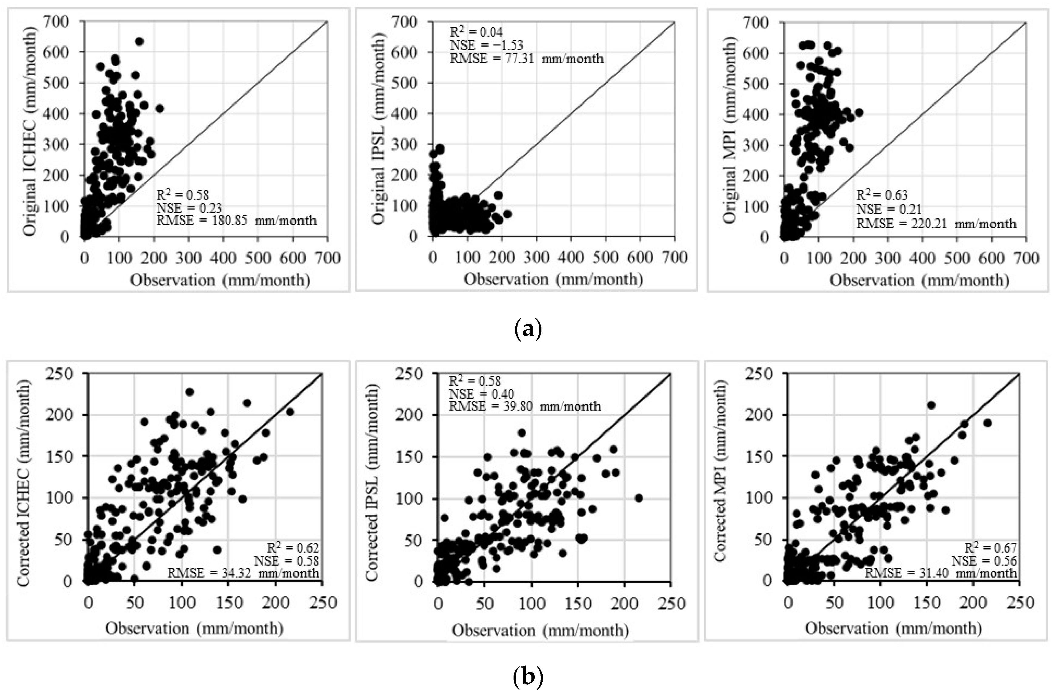
4.3.1. Bias Correction of RCMs

Quantile mapping is a statistical technique that can be used to correct biases in RCMs. The cumulative distribution functions (CDFs) of the RCM were adjusted to align with the CDF of the observed data. In this study, bias correction using the quantile mapping method was applied to the three selected RCMs. Examples of the results of bias correction for the RCMs over the period of 1986–2005 are provided in Figure 7 and Figure 8. Figure 7 presents how closely the monthly precipitation from RCMs fits with the observations, while Figure 8 shows how much the correlation between the RCMs and observations can be improved after bias correction. The quantile mapping method was found to reduce bias and improve the monthly precipitation for all of the selected RCMs. A large improvement in adjusting the RCM’s precipitation was achieved for the ICHEC and MPI when the extreme precipitation values approximately over 600 mm could be reduced close to the maximum observation around 215 mm. After bias correction, the values of R2, NSE, and RMSE of the three RCMs’ ranged from 0.58 to 0.67, from 0.40 to 0.63, and from 31.40 to 39.80 mm/month. The MPI yielded the best performance with the highest values, namely R2 = 0.67, NSE = 0.63, and RMSE = 31.40 mm/month, followed by IPSL and ICHEC. It is important to note that, while the empirical quantile mapping method was proven to perform satisfactorily for this study, the results could be sensitive to the choice of calibration time period [78]. The choice of the best RCM may then be altered when the future state of climate becomes unpredictable due to several factors involving a chaotic system, such as uncertainty, randomness, and the divergence from initial conditions as it moves beyond a time horizon [79,80]. Thus, the robustness of the bias correction method applied here cannot be guaranteed and it is less decisive on the choice of the RCM.

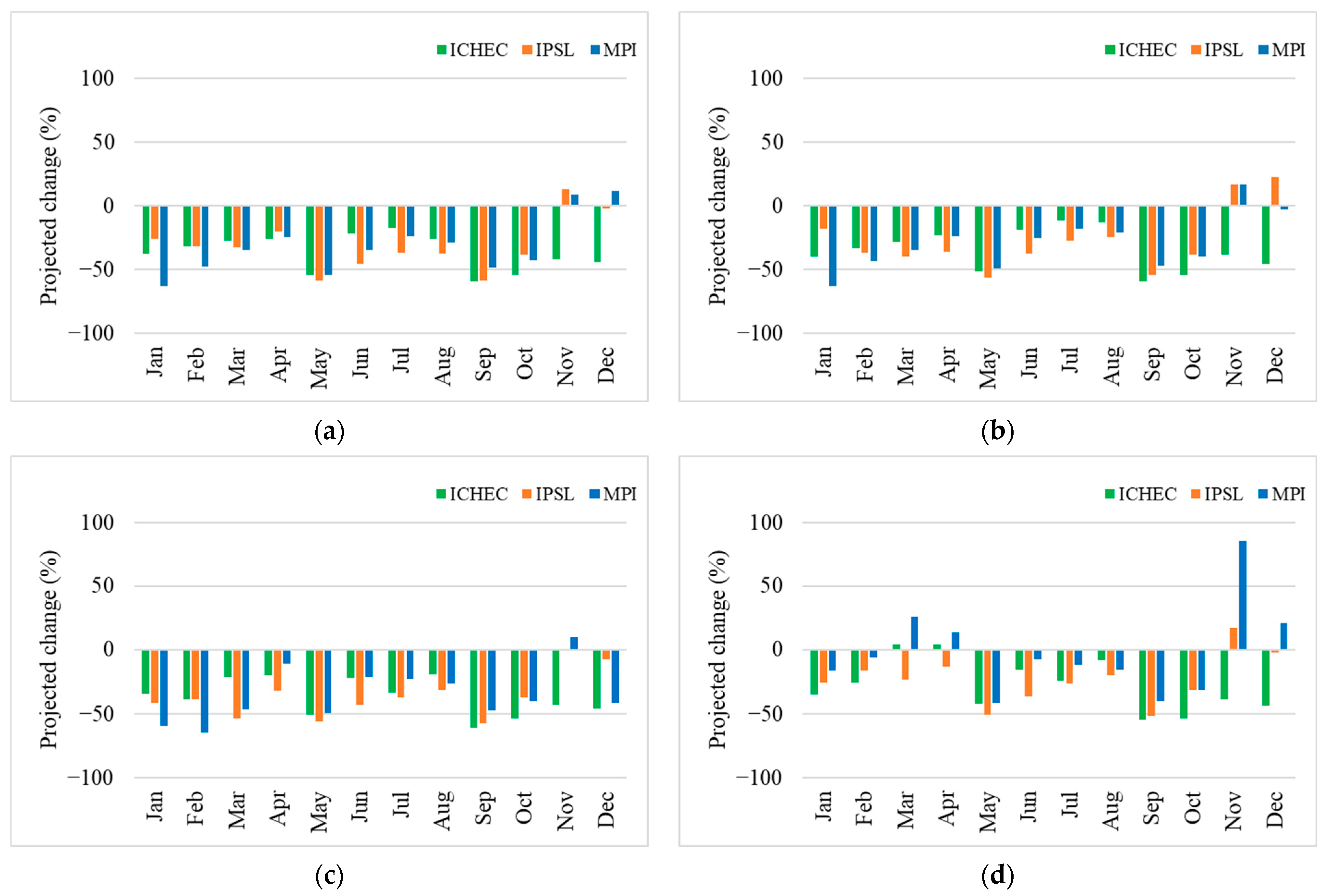
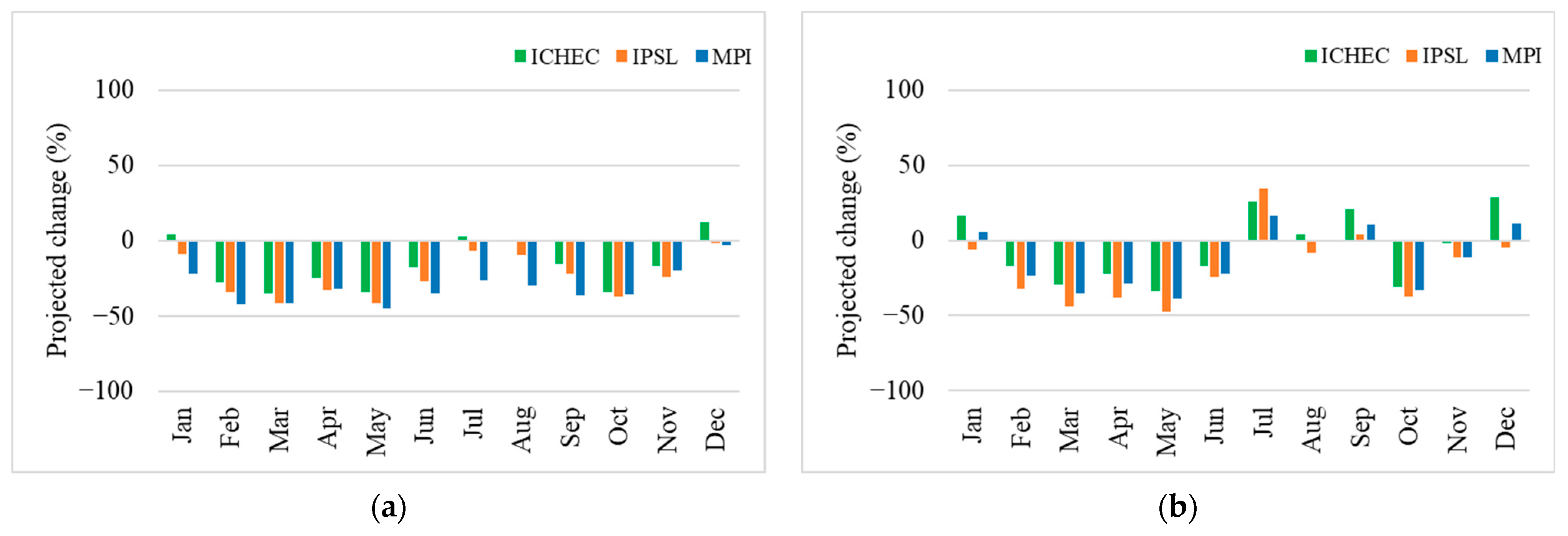
4.3.2. Changes in the Future Precipitation and Streamflow

The bias-corrected precipitation from the ICHEC, IPSL, and MPI was input into the calibrated SWAT model to simulate streamflow in the near future (2025–2049) and far future (2075–2099) periods. Figures showing the monthly average precipitation and streamflow in the baseline and future periods obtained from the three RCMs are provided in Appendix A.
The projected changes in future precipitation and streamflow, which were compared with the monthly average values in the baseline period of 1986–2016, are shown in Figure 9 and Figure 10 and Table 4. Figure 9 indicates that the projected precipitation obtained from all RCMs generally decreases for almost all months in both periods and both climate scenarios. Particularly, rainfall in the wet months of May and September reduces by about 50% for all models and all scenarios. A milder increase of 8–22% in dry season precipitation was found for RCP4.5 (Figure 9a,b), while a larger increase of up to 85% could occur under RCP8.5 in the far future, especially when the MPI was used (Figure 9d). The differences in the projected changes in the monthly average precipitation in the near and far futures are more noticeable for RCP8.5 than for RCP4.5.
Figure 10a shows that the projected streamflow decreases in most months in the near future period under RCP4.5. This pattern of change corresponds with the change in the projected precipitation under the same condition. The changes in the projected monthly streamflow are highly variable when moving from the near to far future period and from low to high trajectory. The streamflow under RCP8.5 in the far future (Figure 10d) shows an opposite change to the precipitation (Figure 9d) in several months. This is probably due to a combined effect of a milder decrease in projected precipitation in the far future under RCP8.5 and an insufficient representation of evaporation due to a warmer climate, which can be considered the limitation of this study. Changes in annual streamflow are shown in Table 5.
Changes in the future precipitation and streamflow were also detected in other basins influenced by similar climate regimes. For example, under the impact of climate change scenario RCP 8.5 of the four RCMs (HadGEM3-RA, SNU-MM5, RegCM4, and YSU-RSM), the streamflow in the Srepok Basin, Vietnam in the future period of 2016–2040 would be expected to decrease by about 12% due to a decrease in precipitation and an increase in evapotranspiration [75]. A reduction in the projected precipitation and streamflow is likely to induce higher risk of drought and make the CPRB more vulnerable in the future. Thus, the future management of drought would require more stringent measures to deal with uncertainty and possibly more severe drought conditions.

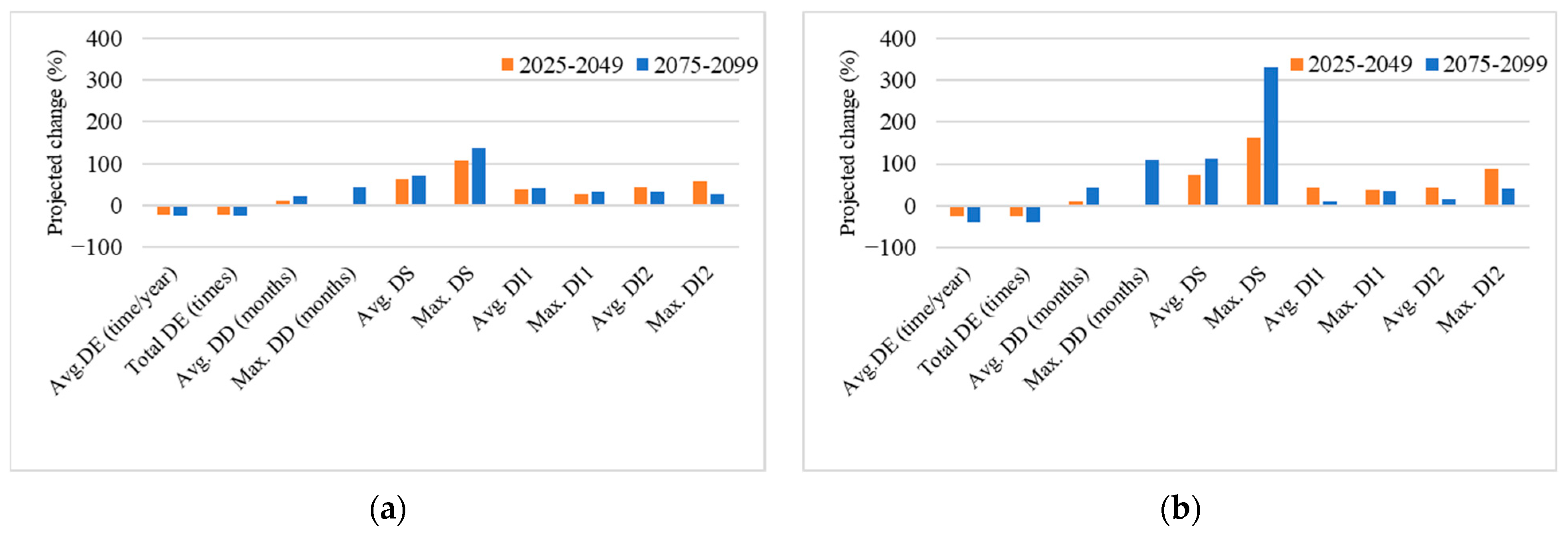
4.3.3. Future Drought Characteristics

This section discusses how climate change can influence future drought characteristics. The results based on MPI form the predominant part of this section. Additional results shown in Appendix B allow for a further investigation of the SPI and SSI developed from ICHEC and IPSL.
Figure 11 shows the temporal variation in the SPI and SSI in the future periods obtained from the MPI model. The lag of responses is not clear. The relationship between the SPI and SSI is much deteriorated, suggesting a substantial change in the future drought signal as it moves from meteorological to hydrological drought. The propagation of drought through the hydrological cycle would be less predictable, especially for the near future period when the maximum r value at a 12-month time scale is only 0.39 for RCP8.5 (Figure 11c). Higher r values can be obtained when ICHEC or IPSL are used (see Figure A3 and Figure A4). Similar difficulty in translating meteorological to hydrological drought was also discussed in [74].
A poor relationship between the SPI and SSI is found for short and medium time scales. Better agreement between the SPI and SSI is obtained for a long time scale. The relationships between the SPI and SSI are relatively high for the baseline and far future and lower for the near future period. The agreement in this tendency was for all RCMs, as seen in Figure 11, Figure A3, and Figure A4. The cause of these fluctuations is unclear, but it is probably due to the randomness that is typically associated with the inherent unpredictability of future climate phenomena [79,81].
The frequency of hydro-meteorological drought would decrease in both near and far future periods. A strong temporal fluctuation with alternating wet and dry conditions can be seen from the values of SPI and SSI at all time scales varying in a wide range. As can be seen in Figure 11a, for RCP4.5, 2039–2043 and 2046–2048 are the periods of major hydro-meteorological drought events with a long duration and high severity. For RCP8.5, as shown in Figure 11c, the period of major hydro-meteorological drought is expected to come earlier during 2028 and 2032.
For the near future period, the longest meteorological and hydrological durations are 52 and 61 months, accordingly. The lowest SPI and SSI are −3.10 and −1.80, respectively. Figure 11b–d show that the meteorological drought duration in the far future will generally be shorter. Its maximum drought duration would reduce from the near future period to 47 months. The lowest SPI is −3.18, which is similar to the value in the near future period. The hydrological drought conditions would not change much from their conditions in the near future period. The maximum period of hydrological drought and the lowest SSI in the far future are 61 months and −1.75, accordingly.
However, these analyses of droughts were primarily based on a single RCM and may not yet provide a robust implication of the future evolution of hydro-meteorological drought. In addition, randomness and uncertainty from other sources such as the unpredictability of natural and anthropogenic forcings and nonlinearities in the climate system that cannot be fully accounted for by the methods or models used in this study may limit the interpretation of the obtained results.
The projected changes in the characteristics of the meteorological and hydrological droughts in the near and far future periods are shown in Figure 12 and Figure 13, which are represented by the drought parameters calculated over a 6-month time scale, as it was suggested to be the appropriate time scale for drought characterization [63,76,77]. The projected changes in SPI6 and SSI6 were compared to those of the baseline period of 1986–2016.
Figure 12 shows that the projected meteorological drought would occur less frequently but last for a longer duration with a higher intensity and severity in both periods and both climate scenarios. The change in maximum severity could be as high as 330% compared to that of the baseline period. This is believed to be caused by a decrease in the projected rainfall, as explained in Section 4.3.2. Although the decrease in precipitation for the 2075–2099 period under RCP8.5 was less than that under RCP4.5 (Figure 9b) and the decrease in precipitation for the 2075–2099 period was less than that for the 2025–2049 period, the longest drought duration of 48 months from April 2076 to March 2080 that would occur under RCP8.5 led to the maximum severity of 330%. This is because the SPI values can be summed up over the longest duration of 48 months compared to a shorter duration of over 22 months (May 2030 to Feb 2032) for RCP8.5 in the near future and over 33 months (May 2077 to Jan 2080) for RCP4.5 in the far future.
Figure 13 shows that the projected change in hydrological drought characteristics is smaller than that of the meteorological drought. Under RCP4.5, the number of drought events would reduce in the near future but increase in the far future. The drought would be shorter and less severe than a historical drought. For RCP8.5, droughts tend to be less frequent and less severe. However, the intensity could be higher for both future periods. The results reveal that climate change has the potential to alter drought behavior. While it is noted that another variable, such as groundwater, might have an important role in the drought process, the results presented in this study primarily rely on precipitation and streamflow, which are simple but informative.

5. Conclusions

This study aims to investigate the characteristics of hydro-meteorological droughts and possible alterations caused by climate change in the CPRB using the SWAT model, RCMs, and drought indices.
The main findings concluded from this study are as follows: (1) The bias-corrected MPI fits best with the observations of the CPRB when compared to IPSL and ICHEC. (2) The SWAT model performs sufficiently well in simulating streamflow in the CPRB under future climate scenarios. (3) The characteristics of historical drought in the CPRB are associated with the seasonal rainfall pattern; hydro-meteorological droughts were often found during the dry months, and the lag between meteorological and hydrological droughts is approximately 1–3 months depending on the time scales. (4) Climate change was found to alter the hydro-meteorological drought behaviors in the CPRB; meteorological drought tends to be affected more than hydrological drought in both future periods and under both scenarios. This is possibly due to the role of the soil moisture and baseflow that retards the change in the streamflow.
The findings from this study offer a more comprehensive understanding of future hydro-meteorological droughts over the CPRB where droughts have long been overlooked. Using limited numbers of rainfall events, streamflow gauges, and RCMs and presenting the results based on the spatially averaged values of the drought indices greatly limit the ability to characterize drought conditions on a local scale.
Future studies should increase the number of gauging stations or incorporate a high resolution of satellite-based products into the analysis, and it is strongly encouraged to use the ensemble mean to represent the multi-RCM results and add more hydrological variables to calculate drought indices that could offer a more reliable characterization of droughts, especially on local and regional scales. This study has contributed to an improved understanding and characterization of droughts over the CPRB. Valuable findings based on this study can be used to support water resource management decision making during droughts.

Author Contributions

Conceptualization, S.V.; Data Curation, B.K. and P.P.; Formal Analysis, B.K. and P.P.; Funding Acquisition, S.V.; Investigation, B.K.; Methodology, B.K. and S.V.; Project Administration, S.V.; Resources, C.E. and S.V.; Software, P.P.; Supervision, S.V.; Validation, C.E.; Visualization, P.P.; Writing—Original Draft, B.K.; Writing—Review and Editing, C.E. and S.V. All authors have read and agreed to the published version of the manuscript.

Funding

This research was funded by Thailand Science research and Innovation Fund Chulalongkorn University (CU_FRB65_dis (24)_149_21_15).

Data Availability Statement

The data presented in this study are available on request from the corresponding author. The data are not publicly available due to their intended use for educational purposes within specific academic research.

Acknowledgments

The authors would like to express our gratitude to Chulalongkorn University for providing financial support for this work. We are grateful to the Thai Meteorological Department (TMD), Royal Irrigation Department (RID), Land Development Department (LDD), SEACLID/CORDEX-SEA project, and U.S. Geological Survey for providing access to the data that made this research possible. We would like to acknowledge the helpful comments and suggestions made by the anonymous reviewers, which greatly improved the quality of this paper.

Conflicts of Interest

The authors declare no conflict of interest.

Appendix A

This appendix provides figures of the monthly average precipitation and streamflow in the baseline and future periods produced from ICHEC, IPSL, and MPI.
Figure A1. Monthly average precipitation over CPRB in baseline and future periods. (a) RCP4.5 near future scenario; (b) RCP4.5 far future scenario; (c) RCP8.5 near future scenario; (d) RCP8.5 far future scenario.
Water 16 01023 g0a1
Figure A2. Monthly average streamflow over CPRB calculated from average streamflow at stations P.1, W.1A, Y.1A, N.1, and C.2 in baseline and future periods. (a) RCP4.5 near future scenario; (b) RCP4.5 far future scenario; (c) RCP8.5 near future scenario; (d) RCP8.5 far future scenario.
Water 16 01023 g0a2

Appendix B

This appendix provides figures of the temporal variation in the spatial averaged time series for the SPI and SSI in the future periods produced from ICHEC and IPSL.
Figure A3. Temporal variation in spatial averaged time series for SPI and SSI over CPRB at 3-, 6-, and 12-month time scales calculated based on ICHEC model in future periods. (a) RCP4.5 near future scenario; (b) RCP4.5 far future scenario; (c) RCP8.5 near future scenario; (d) RCP8.5 far future scenario. Color scale moving from yellow to red represents mild, moderate, severe, and extreme drought categories, respectively.
Water 16 01023 g0a3aWater 16 01023 g0a3b
Figure A4. Temporal variation in spatial averaged time series for SPI and SSI over CPRB at 3-, 6-, and 12-month time scales calculated based on IPSL model in future periods. (a) RCP4.5 near future scenario; (b) RCP4.5 far future scenario; (c) RCP8.5 near future scenario; (d) RCP8.5 far future scenario. Color scale moving from yellow to red represents mild, moderate, severe, and extreme drought categories, respectively.
Water 16 01023 g0a4aWater 16 01023 g0a4b

References

  1. Centre for Research on the Epidemiology of Disaster (CRED). 2021 Disasters in Numbers; CRED: Brussels, Belgium, 2022. [Google Scholar]
  2. World Economic Forum. The Global Risks Report 2021; World Economic Forum: Geneva, Switzerland, 2021. [Google Scholar]
  3. World Meteorological Organization (WMO); Global Water Partnership (GWP). Handbook of Drought Indicators and Indices; WMO: Geneva, Switzerland, 2016. [Google Scholar]
  4. Wilhite, D.A. Drought. In Encyclopedia of World Climatology; Oliver, J.E., Ed.; Springer: Dordrecht, The Netherlands, 2005; pp. 338–341. [Google Scholar]
  5. Mishra, A.K.; Singh, V.P. A review of drought concepts. J. Hydrol. 2010, 391, 202–216. [Google Scholar] [CrossRef]
  6. Singh, C.; Jain, G.; Sukhwani, V.; Shaw, R. Losses and damages associated with slow-onset events: Urban drought and water insecurity in Asia. Curr. Opin. Environ. Sustain. 2021, 50, 72–86. [Google Scholar] [CrossRef]
  7. Wilhite, D.A.; Svoboda, M.D.; Hayes, M.J. Understanding the complex impacts of drought: A key to enhancing drought mitigation and preparedness. Water Resour. Manag. 2007, 21, 763–774. [Google Scholar] [CrossRef]
  8. Hayes, M.J.; Wilhelmi, O.V.; Knutson, C.L. Reducing Drought Risk: Bridging Theory and Practice. Nat. Hazards Rev. 2004, 5, 106–113. [Google Scholar] [CrossRef]
  9. Khadka, D.; Babel, M.S.; Shrestha, S.; Virdis, S.G.P.; Collins, M. Multivariate and multi-temporal analysis of meteorological drought in the northeast of Thailand. Weather Clim. Extrem. 2021, 34, 100399. [Google Scholar] [CrossRef]
  10. Kongjun, T. Water Management in The Chao Phraya River Basin during Drought Crisis. Natl. Def. Coll. Thail. J. 2018, 60, 127–155. [Google Scholar]
  11. Pandey, S.; Bhandari, H.; Hardy, B. Economic Costs of Drought and Rice Farmers’ Coping Mechanisms: A Cross-Country Comparative Analysis; International Rice Research Institute (IRRI): Los Baños, Philippines, 2007. [Google Scholar]
  12. Buckley, B.M.; Palakit, K.; Duangsathaporn, K.; Sanguantham, P.; Prasomsin, P. Decadal scale droughts over northwestern Thailand over the past 448 years: Links to the tropical Pacific and Indian Ocean sectors. Clim. Dyn. 2007, 29, 63–71. [Google Scholar] [CrossRef]
  13. Thavorntam, W.; Tantemsapya, N.; Armstrong, L. A combination of meteorological and satellite-based drought indices in a better drought assessment and forecasting in Northeast Thailand. Nat. Hazards 2015, 77, 1453–1474. [Google Scholar] [CrossRef]
  14. Homdee, T.; Pongput, K.; Kanae, S. A comparative performance analysis of three standardized climatic drought indices in the Chi River basin, Thailand. Agric. Nat. Resour. 2016, 50, 211–219. [Google Scholar] [CrossRef]
  15. Laosuwan, T.; Sangpradid, S.; Gomasathit, T.; Rotjanakusol, T. Application of remote sensing technology for drought monitoring in Mahasarakham Province, Thailand. Int. J. Geoinform. 2016, 12, 17–25. [Google Scholar]
  16. Wichitarapongsakun, P.; Sarin, C.; Klomjek, P.; Chuenchooklin, S. Rainfall prediction and meteorological drought analysis in the Sakae Krang River basin of Thailand. Agric. Nat. Resour. 2016, 50, 490–498. [Google Scholar] [CrossRef]
  17. Prabnakorn, S.; Maskey, S.; Suryadi, F.X.; de Fraiture, C. Rice yield in response to climate trends and drought index in the Mun River Basin, Thailand. Sci. Total Environ. 2018, 621, 108–119. [Google Scholar] [CrossRef] [PubMed]
  18. Singhrattna, N.; Rajagopalan, B.; Kumar, K.K.; Clark, M. Interannual and Interdecadal Variability of Thailand Summer Monsoon Season. J. Clim. 2005, 18, 1697–1708. [Google Scholar] [CrossRef]
  19. Pratoomchai, W.; Ekkawatpanit, C.; Yoobanpot, N.; Lee, K.T. A Dilemma between Flood and Drought Management: Case Study of the Upper Chao Phraya Flood-Prone Area in Thailand. Water 2022, 14, 4056. [Google Scholar] [CrossRef]
  20. Arnold, J.G.; Srinivasan, R.; Muttiah, R.S.; Williams, J.R. Large Area Hydrologic Modeling and Assessment Part I: Model Development1. JAWRA J. Am. Water Resour. Assoc. 1998, 34, 73–89. [Google Scholar] [CrossRef]
  21. Arnold, J.G.; Moriasi, D.N.; Gassman, P.W.; Abbaspour, K.C.; White, M.J.; Srinivasan, R.; Santhi, C.; Harmel, R.D.; van Griensven, A.; Van Liew, M.W.; et al. SWAT: Model Use, Calibration, and Validation. Trans. ASABE 2012, 55, 1491–1508. [Google Scholar] [CrossRef]
  22. Neitsch, A.L.; Arnold, J.G.; Kiniry, J.R.; Williams, J.R. Soil and Water Assessment Tool: Theoretical Documentation Version 2009; Texas A&M University: College Station, TX, USA, 2011. [Google Scholar]
  23. Gassman, P.W.; Reyes, M.R.; Green, C.H.; Arnold, J.G. The Soil and Water Assessment Tool: Historical Development, Applications, and Future Research Directions. Trans. ASABE 2007, 50, 1211–1250. [Google Scholar] [CrossRef]
  24. Khoi, D.N.; Sam, T.T.; Loi, P.T.; Hung, B.V.; Nguyen, V.T. Impact of climate change on hydro-meteorological drought over the Be River Basin, Vietnam. J. Water Clim. Change 2021, 12, 3159–3169. [Google Scholar] [CrossRef]
  25. Tan, M.L.; Gassman, P.W.; Yang, X.; Haywood, J. A review of SWAT applications, performance and future needs for simulation of hydro-climatic extremes. Adv. Water Resour. 2020, 143, 103662. [Google Scholar] [CrossRef]
  26. Visessri, S.; McIntyre, N. Regionalisation of hydrological responses under land-use change and variable data quality. Hydrol. Sci. J. 2016, 61, 302–320. [Google Scholar] [CrossRef]
  27. Tan, M.L.; Gassman, P.W.; Srinivasan, R.; Arnold, J.G.; Yang, X. A Review of SWAT Studies in Southeast Asia: Applications, Challenges and Future Directions. Water 2019, 11, 914. [Google Scholar] [CrossRef]
  28. Abbaspour, K.C. SWAT-CUP: SWAT Calibration and Uncertainty Programs—A User Manual; Eawag—Swiss Federal Institute of Aquatic Science and Technology: Dübendorf, Switzerland, 2015. [Google Scholar]
  29. Rafiei Emam, A.; Kappas, M.; Fassnacht, S.; Linh, N.H.K. Uncertainty analysis of hydrological modeling in a tropical area using different algorithms. Front. Earth Sci. 2018, 12, 661–671. [Google Scholar] [CrossRef]
  30. Moriasi, D.; Gitau, M.; Pai, N.; Daggupati, P. Hydrologic and Water Quality Models: Performance Measures and Evaluation Criteria. Trans. ASABE (Am. Soc. Agric. Biol. Eng.) 2015, 58, 1763–1785. [Google Scholar] [CrossRef]
  31. Moriasi, D.; Arnold, J.; Van Liew, M.; Bingner, R.; Harmel, R.D.; Veith, T. Model Evaluation Guidelines for Systematic Quantification of Accuracy in Watershed Simulations. Trans. ASABE 2007, 50, 885–900. [Google Scholar] [CrossRef]
  32. Tangang, F.; Chung, J.X.; Juneng, L.; Supari; Salimun, E.; Ngai, S.T.; Jamaluddin, A.F.; Mohd, M.S.F.; Cruz, F.; Narisma, G.; et al. Projected future changes in rainfall in Southeast Asia based on CORDEX–SEA multi-model simulations. Clim. Dyn. 2020, 55, 1247–1267. [Google Scholar] [CrossRef]
  33. Tapiador, F.J.; Navarro, A.; Moreno, R.; Sánchez, J.L.; García-Ortega, E. Regional climate models: 30 years of dynamical downscaling. Atmos. Res. 2020, 235, 104785. [Google Scholar] [CrossRef]
  34. Caillaud, C.; Somot, S.; Alias, A.; Bernard-Bouissières, I.; Fumière, Q.; Laurantin, O.; Seity, Y.; Ducrocq, V. Modelling Mediterranean heavy precipitation events at climate scale: An object-oriented evaluation of the CNRM-AROME convection-permitting regional climate model. Clim. Dyn. 2021, 56, 1717–1752. [Google Scholar] [CrossRef]
  35. Giorgi, F. Thirty Years of Regional Climate Modeling: Where Are We and Where Are We Going next? J. Geophys. Res. Atmos. 2019, 124, 5696–5723. [Google Scholar] [CrossRef]
  36. Wang, Y.; Leung, L.R.; McGregor, J.L.; Lee, D.-K.; Wang, W.-C.; Ding, Y.; Kimura, F. Regional Climate Modeling: Progress, Challenges, and Prospects. J. Meteorol. Soc. Jpn. Ser. II 2004, 82, 1599–1628. [Google Scholar] [CrossRef]
  37. Lee, D.-K.; Cha, D.-H. Regional climate modeling for Asia. Geosci. Lett. 2020, 7, 13. [Google Scholar] [CrossRef]
  38. Lee, D.-K.; Cha, D.-H.; Jin, C.-S.; Choi, S.-J. A regional climate change simulation over East Asia. Asia-Pac. J. Atmos. Sci. 2013, 49, 655–664. [Google Scholar] [CrossRef]
  39. Takle, E.S.; Gutowski, W.J., Jr.; Arritt, R.W.; Pan, Z.; Anderson, C.J.; da Silva, R.R.; Caya, D.; Chen, S.-C.; Giorgi, F.; Christensen, J.H.; et al. Project to Intercompare Regional Climate Simulations (PIRCS): Description and initial results. J. Geophys. Res. Atmos. 1999, 104, 19443–19461. [Google Scholar] [CrossRef]
  40. Fu, C.; Wang, S.; Xiong, Z.; Gutowski, W.J.; Lee, D.-K.; McGregor, J.L.; Sato, Y.; Kato, H.; Kim, J.-W.; Suh, M.-S. Regional Climate Model Intercomparison Project for Asia. Bull. Am. Meteorol. Soc. 2005, 86, 257–266. [Google Scholar] [CrossRef]
  41. Herrmann, M.; Ngo-Duc, T.; Trinh-Tuan, L. Impact of climate change on sea surface wind in Southeast Asia, from climatological average to extreme events: Results from a dynamical downscaling. Clim. Dyn. 2020, 54, 2101–2134. [Google Scholar] [CrossRef]
  42. Juneng, L.; Tangang, F.; Chung, J.X.; Ngai, S.T.; Tay, T.W.; Narisma, G.; Cruz, F.; Phan-Van, T.; Ngo-Duc, T.; Santisirisomboon, J.; et al. Sensitivity of Southeast Asia rainfall simulations to cumulus and air-sea flux parameterizations in RegCM4. Clim. Res. 2016, 69, 59–77. [Google Scholar] [CrossRef]
  43. Ngo-Duc, T.; Tangang, F.T.; Santisirisomboon, J.; Cruz, F.; Trinh-Tuan, L.; Nguyen-Xuan, T.; Phan-Van, T.; Juneng, L.; Narisma, G.; Singhruck, P.; et al. Performance evaluation of RegCM4 in simulating extreme rainfall and temperature indices over the CORDEX-Southeast Asia region. Int. J. Climatol. 2017, 37, 1634–1647. [Google Scholar] [CrossRef]
  44. Supari; Tangang, F.; Juneng, L.; Cruz, F.; Chung, J.X.; Ngai, S.T.; Salimun, E.; Mohd, M.S.F.; Santisirisomboon, J.; Singhruck, P.; et al. Multi-model projections of precipitation extremes in Southeast Asia based on CORDEX-Southeast Asia simulations. Environ. Res. 2020, 184, 109350. [Google Scholar] [CrossRef] [PubMed]
  45. Trinh-Tuan, L.; Matsumoto, J.; Tangang, F.T.; Juneng, L.; Cruz, F.; Narisma, G.; Santisirisomboon, J.; Phan-Van, T.; Gunawan, D.; Aldrian, E.; et al. Application of Quantile Mapping Bias Correction for Mid-Future Precipitation Projections over Vietnam. SOLA 2019, 15, 1–6. [Google Scholar] [CrossRef]
  46. Hirota, N.; Takayabu, Y.N. Reproducibility of precipitation distribution over the tropical oceans in CMIP5 multi-climate models compared to CMIP3. Clim. Dyn. 2013, 41, 2909–2920. [Google Scholar] [CrossRef]
  47. Mehran, A.; AghaKouchak, A.; Phillips, T.J. Evaluation of CMIP5 continental precipitation simulations relative to satellite-based gauge-adjusted observations. J. Geophys. Res. Atmos. 2014, 119, 1695–1707. [Google Scholar] [CrossRef]
  48. Campozano, L.; Ballari, D.; Montenegro, M.; Avilés, A. Future Meteorological Droughts in Ecuador: Decreasing Trends and Associated Spatio-Temporal Features Derived From CMIP5 Models. Front. Earth Sci. 2020, 8, 17. [Google Scholar] [CrossRef]
  49. Jin, C.-S.; Cha, D.-H.; Lee, D.-K.; Suh, M.-S.; Hong, S.-Y.; Kang, H.-S.; Ho, C.-H. Evaluation of climatological tropical cyclone activity over the western North Pacific in the CORDEX-East Asia multi-RCM simulations. Clim. Dyn. 2016, 47, 765–778. [Google Scholar] [CrossRef]
  50. Kim, J.; Waliser, D.E.; Mattmann, C.A.; Goodale, C.E.; Hart, A.F.; Zimdars, P.A.; Crichton, D.J.; Jones, C.; Nikulin, G.; Hewitson, B.; et al. Evaluation of the CORDEX-Africa multi-RCM hindcast: Systematic model errors. Clim. Dyn. 2014, 42, 1189–1202. [Google Scholar] [CrossRef]
  51. Kendon, E.J.; Jones, R.G.; Kjellström, E.; Murphy, J.M. Using and Designing GCM–RCM Ensemble Regional Climate Projections. J. Clim. 2010, 23, 6485–6503. [Google Scholar] [CrossRef]
  52. Torma, C.; Giorgi, F.; Coppola, E. Added value of regional climate modeling over areas characterized by complex terrain—Precipitation over the Alps. J. Geophys. Res. Atmos. 2015, 120, 3957–3972. [Google Scholar] [CrossRef]
  53. Sanderson, B.; Knutti, R. Climate ChangeclimatechangeProjectionsclimatechangeprojections: Characterizing Uncertainty Using Climate Models. In Encyclopedia of Sustainability Science and Technology; Meyers, R.A., Ed.; Springer: New York, NY, USA, 2012; pp. 2097–2114. [Google Scholar]
  54. Eckel, F.A.; Allen, M.S.; Sittel, M.C. Estimation of Ambiguity in Ensemble Forecasts. Weather Forecast. 2012, 27, 50–69. [Google Scholar] [CrossRef]
  55. Ngai, S.T.; Tangang, F.; Juneng, L. Bias correction of global and regional simulated daily precipitation and surface mean temperature over Southeast Asia using quantile mapping method. Glob. Planet. Change 2017, 149, 79–90. [Google Scholar] [CrossRef]
  56. Wilhite, D.A.; Glantz, M.H. Understanding: The drought phenomenon: The role of definitions. Water Int. 1985, 10, 111–120. [Google Scholar] [CrossRef]
  57. AghaKouchak, A.; Mirchi, A.; Madani, K.; Di Baldassarre, G.; Nazemi, A.; Alborzi, A.; Anjileli, H.; Azarderakhsh, M.; Chiang, F.; Hassanzadeh, E.; et al. Anthropogenic Drought: Definition, Challenges, and Opportunities. Rev. Geophys. 2021, 59, e2019RG000683. [Google Scholar] [CrossRef]
  58. Guttman, N.B. Comparing the palmer drought index and the standardized precipitation index. JAWRA J. Am. Water Resour. Assoc. 1998, 34, 113–121. [Google Scholar] [CrossRef]
  59. Tsakiris, G.; Vangelis, H. Towards a Drought Watch System based on Spatial SPI. Water Resour. Manag. 2004, 18, 1–12. [Google Scholar] [CrossRef]
  60. Stagge, J.H.; Tallaksen, L.M.; Gudmundsson, L.; Van Loon, A.F.; Stahl, K. Candidate Distributions for Climatological Drought Indices (SPI and SPEI). Int. J. Climatol. 2015, 35, 4027–4040. [Google Scholar] [CrossRef]
  61. Shamshirband, S.; Hashemi, S.; Salimi, H.; Samadianfard, S.; Asadi, E.; Shadkani, S.; Kargar, K.; Mosavi, A.; Nabipour, N.; Chau, K.-W. Predicting Standardized Streamflow index for hydrological drought using machine learning models. Eng. Appl. Comput. Fluid Mech. 2020, 14, 339–350. [Google Scholar] [CrossRef]
  62. Shukla, S.; Wood, A.W. Use of a standardized runoff index for characterizing hydrologic drought. Geophys. Res. Lett. 2008, 35, 1–7. [Google Scholar] [CrossRef]
  63. Salimi, H.; Asadi, E.; Darbandi, S. Meteorological and hydrological drought monitoring using several drought indices. Appl. Water Sci. 2021, 11, 11. [Google Scholar] [CrossRef]
  64. Botai, C.M.; Botai, J.O.; Dlamini, L.C.; Zwane, N.S.; Phaduli, E. Characteristics of Droughts in South Africa: A Case Study of Free State and North West Provinces. Water 2016, 8, 439. [Google Scholar] [CrossRef]
  65. Wu, J.; Chen, X.; Yao, H.; Gao, L.; Chen, Y.; Liu, M. Non-linear relationship of hydrological drought responding to meteorological drought and impact of a large reservoir. J. Hydrol. 2017, 551, 495–507. [Google Scholar] [CrossRef]
  66. Maybank, J.; Bonsai, B.; Jones, K.; Lawford, R.; O’Brien, E.G.; Ripley, E.A.; Wheaton, E. Drought as a natural disaster. Atmos. Ocean 1995, 33, 195–222. [Google Scholar] [CrossRef]
  67. McKee, T.B.; Doesken, N.J.; Kleist, J.R. The Relationship of Drought Frequency and Duration to Time Scales. In Proceedings of the Eight Conference on Applied Climatology, Anaheim, CA, USA, 17–22 January 1993. [Google Scholar]
  68. Jang, D. Assessment of Meteorological Drought Indices in Korea Using RCP 8.5 Scenario. Water 2018, 10, 283. [Google Scholar] [CrossRef]
  69. Sönmez, F.K.; Kömüscü, A.L.I.Ü.; Erkan, A.; Turgu, E. An Analysis of Spatial and Temporal Dimension of Drought Vulnerability in Turkey Using the Standardized Precipitation Index. Nat. Hazards 2005, 35, 243–264. [Google Scholar] [CrossRef]
  70. Guo, H.; Bao, A.; Liu, T.; Ndayisaba, F.; He, D.; Kurban, A.; De Maeyer, P. Meteorological Drought Analysis in the Lower Mekong Basin Using Satellite-Based Long-Term CHIRPS Product. Sustainability 2017, 9, 901. [Google Scholar] [CrossRef]
  71. Yevjevich, V. An Objective Approach to Definitions and Investigations to Continental Hydrologic Droughts; Colorado State University: Fort Collins, CO, USA, 1967. [Google Scholar]
  72. Moyé, L.A.; Kapadia, A.S.; Cech, I.M.; Hardy, R.J. The theory of runs with applications to drought prediction. J. Hydrol. 1988, 103, 127–137. [Google Scholar] [CrossRef]
  73. Hansa, V. Geoinformatic Public Domain System Model “SWAT” in Thailand. Agric. Nat. Resour. 2006, 40, 264–272. [Google Scholar]
  74. Kamali, B.; Houshmand Kouchi, D.; Yang, H.; Abbaspour, K.C. Multilevel Drought Hazard Assessment under Climate Change Scenarios in Semi-Arid Regions—A Case Study of the Karkheh River Basin in Iran. Water 2017, 9, 241. [Google Scholar] [CrossRef]
  75. Sam, T.T.; Khoi, D.N.; Thao, N.T.T.; Nhi, P.T.T.; Quan, N.T.; Hoan, N.X.; Nguyen, V.T. Impact of climate change on meteorological, hydrological and agricultural droughts in the Lower Mekong River Basin: A case study of the Srepok Basin, Vietnam. Water Environ. J. 2019, 33, 547–559. [Google Scholar] [CrossRef]
  76. Spinoni, J.; Naumann, G.; Carrao, H.; Barbosa, P.; Vogt, J. World drought frequency, duration, and severity for 1951–2010. Int. J. Climatol. 2014, 34, 2792–2804. [Google Scholar] [CrossRef]
  77. Törnros, T.; Menzel, L. Leaf area index as a function of precipitation within a hydrological model. Hydrol. Res. 2013, 45, 660–672. [Google Scholar] [CrossRef]
  78. Lafon, T.; Dadson, S.; Buys, G.; Prudhomme, C. Bias correction of daily precipitation simulated by a regional climate model: A comparison of methods. Int. J. Climatol. 2013, 33, 1367–1381. [Google Scholar] [CrossRef]
  79. Thompson, J.M.T.; Sieber, J. Climate predictions: The influence of nonlinearity and randomness. Philos. Trans. R. Soc. A Math. Phys. Eng. Sci. 2012, 370, 1007–1011. [Google Scholar] [CrossRef] [PubMed]
  80. Suzuki-Parker, A.; Kusaka, H.; Takayabu, I.; Dairaku, K.; Ishizaki, N.N.; Ham, S. Contributions of GCM/RCM Uncertainty in Ensemble Dynamical Downscaling for Precipitation in East Asian Summer Monsoon Season. SOLA 2018, 14, 97–104. [Google Scholar] [CrossRef]
  81. Montanari, A.; Koutsoyiannis, D. A blueprint for process-based modeling of uncertain hydrological systems. Water Resour. Res. 2012, 48, 1–15. [Google Scholar] [CrossRef]
Figure 1. The location, topography, river network, and hydro-meteorological gauges of the study area.
Water 16 01023 g001
Figure 2. A schematic diagram of the overall framework.
Water 16 01023 g002
Figure 3. A Theory of Runs illustration of a drought event and the drought indicators [70].
Water 16 01023 g003
Figure 4. Daily hydrographs of observed and simulated streamflow for calibration (1986–1995) and validation (1996–2005) periods at five stations in CPRB.
Water 16 01023 g004
Figure 5. The temporal variation in spatial averaged time series for the SPI and SSI over the CPRB at 3-, 6-, and 12-month time scales calculated based on the period of 1986–2016. A color scale moving from yellow to red represents mild, moderate, severe, and extreme drought categories, respectively.
Water 16 01023 g005
Figure 6. Cross-correlation function of SPI and SSI for 3-, 6-, and 12-month accumulation periods.
Water 16 01023 g006
Figure 7. Comparison of monthly average observed and RCM precipitation (a) before bias correction and (b) after bias correction.
Water 16 01023 g007
Figure 8. Relationship between observed and modeled RCMs’ precipitation (a) before bias correction; (b) after bias correction.
Water 16 01023 g008
Figure 9. Relative change in monthly average precipitation. (a) RCP4.5 near future scenario; (b) RCP4.5 far future scenario; (c) RCP8.5 near future scenario; (d) RCP8.5 far future scenario.
Water 16 01023 g009
Figure 10. Relative change in monthly average streamflow. (a) RCP4.5 near future scenario; (b) RCP4.5 far future scenario; (c) RCP8.5 near future scenario; (d) RCP8.5 far future scenario.
Water 16 01023 g010aWater 16 01023 g010b
Figure 11. Temporal variation of spatial averaged time series for SPI and SSI over CPRB at 3-, 6- and 12-month time scales calculated based on MPI model. (a) RCP4.5 near future scenario; (b) RCP 4.5 far future scenario; (c) RCP8.5 near future scenario; (d) RCP8.5 far future scenario. Color scale moving from yellow to red represents mild, moderate, severe, and extreme drought categories, respectively.
Water 16 01023 g011aWater 16 01023 g011bWater 16 01023 g011c
Figure 12. Relative change in SPI6 based on MPI model. (a) RCP4.5 scenario; (b) RCP8.5 scenario.
Water 16 01023 g012
Figure 13. Relative change in SSI6 based on MPI model. (a) RCP4.5 scenario; (b) RCP8.5 scenario.
Water 16 01023 g013
Table 1. Summary of data used in this study.
DataPeriodSpatial
Resolution
Source
Observed rainfall1986–2016PointThai Meteorological Department (TMD)
Observed streamflow1986–2016PointRoyal Irrigation Department (RID), Thailand
RCMs (MPI, IPSL, ICHEC)1986–2099
2015–2049
2075–2099
25 kmSEACLID/CORDEX-SEA
DEM201930 mSRTM-USGS https://earthexplorer.usgs.gov (accessed on 23 August 2021)
Land use2015100 mLand Development Department (LDD), Thailand
Soil type2007100 mLand Development Department (LDD), Thailand
Table 2. Drought classification.
SPI/SSI Values Drought Category
0 to −0.99Mild drought
−1.00 to −1.49Moderate drought
−1.50 to −1.99Severe drought
≤−2.00Extreme drought
Table 3. Historical drought characteristics in the CPRB represented by the SPI and SSI for 3-, 6-, and 12-month accumulation periods.
Meteorological DroughtHydrological Drought
SPI3SPI6SPI12SSI3SSI6SSI12
Average drought event (time/year)1.521.000.420.900.650.26
Total number of drought events (times)47311328208
Average drought duration (months)3.795.8114.236.689.2522.50
Maximum drought duration (months)232347304661
Average drought severity−1.62−2.73−6.40−4.13−5.92−15.03
Maximum drought severity−8.84−12.77−22.55−27.31−40.03−49.22
Average drought intensity based on DI1−0.58−0.59−0.59−0.60−0.57−0.84
Maximum drought intensity based on DI1−2.11−1.85−1.19−2.29−2.03−1.88
Average drought intensity based on DI2−0.34−0.34−0.31−0.33−0.30−0.45
Maximum drought intensity based on DI2−1.27−0.81−0.75−1.05−0.94−0.85
Table 4. Changes in annual precipitation (in mm).
RCP or RCMNear FutureFar Future
ICHECIPSLMPIICHECIPSLMPI
RCP4.5−440.76−489.15−422.55−395.19−434.06−367.14
RCP8.5−445.95−486.02−381.73−345.80−378.55−210.81
Table 5. Changes in annual streamflow (in m3/s).
RCP or RCMNear FutureFar Future
ICHECIPSLMPIICHECIPSLMPI
RCP4.5−377.51−538.27−703.28−76.10−337.67−234.20
RCP8.5−171.48−369.67−435.37423.0819.78109.98
Disclaimer/Publisher’s Note: The statements, opinions and data contained in all publications are solely those of the individual author(s) and contributor(s) and not of MDPI and/or the editor(s). MDPI and/or the editor(s) disclaim responsibility for any injury to people or property resulting from any ideas, methods, instructions or products referred to in the content.

