Prediction of Soil Erosion Using 3D Point Scans and Acoustic Emissions

Abstract

Over half of the approximately 12,000 earthen watershed dams sponsored by the USDA have exceeded their planned 50-year service life. Age, land use changes, extreme weather events, structural deterioration, and sedimentation filling flood pools pose increased risks of dam incidents and potential failures. Among various mechanisms leading to integrity issues, soil erosion is of particular concern due to its potential to occur with little warning. The objective of this research is to determine if soil erosion can be predicted using acoustic emissions. A simulated dam overtopping experiment was replicated in a test flume with dimensions of 0.61 m by 4.27 m (2 ft. by 14 ft.) with a 13.7% slope and a 0.15 m (6 in) layer of inorganic clay (USCS CL) compacted at 17.4% moisture content. A constant flow discharge of 0.07 m³/s (2.37 cfs) was applied to induce erosion. The test was performed until complete failure of the test section occurred. Throughout the experiment, a sonar radar, a 3D scanning total station, and an accelerometer were used to monitor the water level, erosion levels, and vibrations, respectively. The frequency analysis of the water-induced vibrations was compared to measured erosion volumes to determine if in situ vibrations can predict erosion. The results revealed a linear relationship between erosion volume and time, with noticeable changes in the frequency domains as erosion progressed. The outcomes of this research have the potential to provide real-time insights into the integrity of earthen dams concerning erosion, offering a valuable tool for monitoring and maintenance.

1. Introduction

Soil erosion is the process by which soil is moved from one place to another by natural processes or by human or animal intervention. Soil erosion is a concern for earthen dams due to the decrease in structural stability. Based on the Association of State Dam Safety Officials (ASDSO) database of dam incidents collected between 2010 and 2023, there were 1008 earthen constructed dam incidents with more than half occurring due to dam overtopping [1]. According to [2], 73% of earthen dam failure modes are comprised of overtopping or internal erosion. Dam overtopping can cause erosion, slope stability issues, or even breaching in extreme cases, with little to no warning [3]. With dams exceeding their planned service life and their hazard potential classification changing due to commercial and residential development, the need for dam-monitoring technology and incident prediction is necessary [4].

Throughout the years, numerous methods have been used to investigate and quantify earthen dam integrity. The use of geophysical methods, including ground-penetrating radar [5,6,7], electrical resistivity tomography [8,9,10], self-potential [9,10], induced polarization [11,12], and P- and S-wave reflections [10,13] have been used extensively. However, a limitation of these methods is that they often require active participation and/or disturbance of the soil structure for data gathering. Theoretical approaches include the use of analytical [14], numerical [15,16,17,18,19,20,21], and statistical [22,23] models to predict earthen dam integrity with various conditions and time scales. However, each model has specific assumptions and limitations. Analytical models are often too complicated and computationally expensive except for simple generalized models [15]. Numerical models, such as finite element analysis, require extensive experimental parameters to replicate field conditions, but minor parameter variations can have drastic results [14]. Statistical models such as machine learning, artificial neural networks, and Monte Carlo simulations can be used to quantify soil erosion, but require vast amounts of training data (i.e., historical data) to produce viable results [22,23]. For larger dams, historical data are most likely readily available. However, with small earthen dams, historical data are typically not obtainable since they are located in rural areas [4].

Passive and non-destructive testing include remote sensing with satellites and unmanned aerial systems (UASs) [24,25,26], but these methods require extensive validation and are dependent on regions, scales, and specific applications. Passive seismic data and acoustic emissions have been used extensively to predict the internal erosion and seepage of earthen dams and structures through the use of geophones or accelerometers [27,28]. Research has shown that the increase in the rate of magnitude of acoustic emissions can be correlated to internal erosion events [29,30]. Further investigation is required to determine if this methodology can be used to predict surface erosion. Therefore, the objective of this work was to determine if soil erosion can be predicted using acoustic emissions. A novel laboratory approach was developed to replicate dam overtopping in which acoustic emissions, water discharge, and the resulting surface erosion were quantified. The output of this work is a proof-of-concept design in which acoustic emissions can be used as a real-time passive monitoring system for earthen dam integrity.

2. Methodology

2.1. Experimental Apparatus

A 0.61 m-wide (2.0 ft.) and 4.27 m-long (14.0 ft.) test flume was built with a 13.7% slope for the acoustic monitoring of erosion. An accelerometer was placed 1.52 m (5.0 ft.) from the end of the flume to measure vibration in the soil as water discharged over it. Figure 1 shows a schematic of the test flume and the location of the accelerometer and sonar radar sensor.

A 0.15 m (6 in) layer of homogeneous inorganic clay soil (USCS CL with a plasticity index of 12, liquid limit of 26, dry density of 1.87 g/cc, and moisture content of 17.4%) was placed uniformly on the flume covering the accelerometer and compacted using a vibratory plate and hand tamper. The vibrations within the soil were measured using a Dytran 3623A2T submersible triaxial accelerometer (100 mV/g sensitivity and 50 g range) and a KRYPTON 6XSTG data acquisition system at a sampling rate of 10,000 samples/second (10 kHz). The orientation of the accelerometer is shown in Figure 1 in which the z-direction is vertical, the x-direction is parallel to the direction of flow, and the y-direction is perpendicular to the direction of flow.

A gravity head tank provided constant discharge to the test flume, where the height of the water in the head tank was monitored using a Campbell Scientific CS475A Water Radar Sensor to allow for autonomous flow measurements. The height of the water in the head tank was converted to flow rate using a weir flow formula [31] for rectangular contracted weirs (Equation (1)) in which L is the opening width, which was 0.61 m (2 ft.), and H is the water height. This method was compared to an orifice meter coupled with an air–water differential manometer and was confirmed to be within 4% accuracy. Since this method assumes a water height above the soil, the “zero” level was recalibrated after each test to account for erosion in the soil at the inlet of the test flume.

$$\mathrm{Q}=3.247\times \mathrm{L}\times {\mathrm{H}}^{1.48}-\frac{0.566\times {\mathrm{L}}^{1.9}}{1+2\times {\mathrm{L}}^{1.87}}\times {\mathrm{H}}^{1.9}$$

(1)

The 3D point scans were performed using a Leica NOVA MS50 MultiStation combined with digital imaging and 3D laser scanning. The scans had a point resolution of 7.9 points/cm² (50.9 points/in²). The point scans were analyzed using Leica Infinity software to determine the volume differential from the scan intervals. The calculated differential volume references the soil erosion throughout this work. Before each scan, the flow was stopped, allowing the water to drain to reduce reflection noise and improve the scan quality. After the scans were completed, the flow was restarted.

2.2. Vibration Data Analysis

Previous work using acoustic emissions for internal erosion evaluations used sampling rates ranging from 5 to 500 Hz [27,28]. The raw accelerometer data were collected at a high sampling rate of 10 kHz. Since the dynamic rich repose range of such a system is below the 50 Hz range, a much lower sampling rate will be sufficient to describe soil behavior without aliasing. Thus, an investigation of an optimum sampling rate was conducted.

The power spectral density (PSD) of the vibration signals was analyzed for different sampling rates to determine the optimum sampling frequency for erosion detection. The PSD analysis was performed in MATLAB^® using the Welch method, by converting the time domain accelerations to frequency response spectra and computing the PSD of the signal in g²/Hz. The average power of each vibration signal, i.e., band power, was computed to provide further analysis and comparison with erosion. The average power was computed in the range of 0–100 Hz, which represents the area beneath each PSD response that covers the dynamic excitation range of the experimental soil.

3. Results

3.1. Raw Data

The water discharge flow rate and acceleration data are shown in Figure 2 with respect to relative time. At approximately the 6 h mark, a relative spike in accelerations can be seen for all three directions. Coincidently, this spike occurs during a drawdown of the water flow. Therefore, it is assumed that the spike occurred during flow startup. During the 6 h interval, the water discharge is not constant as with the other intervals. This is due to erosion at the inlet of the test flume causing the “zero” level to change while testing occurred. Since the methodology accounted for any changes in the “zero” level after each testing interval, the resulting intervals had relatively constant flow rates. The erosion of the inlet after the 6 h interval is shown in Figure 3c. In Figure 2, the z-direction acceleration has a significant change in magnitude between the 28 and 34 h intervals. During this time, a major amount of soil eroded in a short time frame and will be referred to as the failure point.

An initial point scan was performed before the flow was started, and all subsequent point scans were performed at the end of the testing period of the day at approximate intervals of 6, 11, 16, 22, 28, and 34 h. The vertical lines in the discharge measurements of Figure 2 (i.e., water height drawdown) represent when the flow was stopped, and Figure 4 represents the 3D point cloud scans. The quantified erosion volumes with respect to time are shown in Figure 5. As shown by the linear regression trendline, the erosion values followed a linear relationship with time until the mass erosion event occurred approximately 34 h from when the test was initiated. The testing was considered complete after the massive erosion event, resulting in the exposure of the accelerometer as shown in Figure 6.

3.2. Sampling Rate Analysis

The excitation frequency and vibration response play a significant role in determining an optimal sampling frequency. As a result, the vibration responses before and after erosion should be considered when determining the sampling frequency. The general rule of thumb is that the sampling frequency should be at least 2 or 2.5 higher than the maximum frequency being analyzed. Twenty second intervals at the 1 h mark, i.e., before erosion, were exported at varying sampling rates consisting of 250 Hz, 500 Hz, 1 kHz, 2 kHz, 5 kHz, and the original 10 kHz to determine a sufficient sampling rate for the vibration analysis. Figure 7 represents the acceleration data for all six sampling rates for 20 s at the 1 h time interval.

As shown in Figure 7, distinguishing between the different sampling rates is not straightforward. Therefore, the power spectral density (PSD) was used to convert the time domain data to the frequency domain. The PSD response for the x-, y-, and z-directions during the 1 h time interval is shown in Figure 8.

From Figure 8, all sampling rates appear to be in agreement in all three axes except the 250 Hz sampling rate at frequencies below 1 Hz in the y- and z-directions. To quantify the PSD amplitude for the rest of the frequency range, the average power of the PSD response was determined for each sampling rate in each direction. The average PSD power is presented as a quantified percent difference from the original sampling rate (

Table 1. Percent difference of the average PSD power for each sampling rate compared to the original 10 kHz sampling rate at the 1 h time interval.

Sampling	x-Axis	y-Axis	z-Axis
Rate	% Diff.	% Diff.	% Diff.
250 Hz	0.08%	0.08%	0.07%
500 Hz	0.05%	0.04%	0.04%
1 kHz	0.02%	0.02%	0.07%
2 kHz	0.01%	0.02%	0.04%
5 kHz	0.00%	0.00%	−0.01%
10 kHz	-	-	-

).

As shown in Table 1, all sampling rates are within ±0.08% of the original 10 kHz sampling rate. However, the amplitude of the acceleration and resulting PSD analysis magnifies after erosion occurs during the 34 h time interval (Figure 2). Therefore, the same analysis was performed at the 34 h time interval for the 1 kHz, 5 kHz, and 10 kHz sampling rates (

Table 2. Percent difference of the average PSD power compared to the original sampling rate during the 34 h time interval.

Sampling	x-Axis	y-Axis	z-Axis
Rate	% Diff.	% Diff.	% Diff.
1 kHz	0.02%	0.02%	0.08%
5 kHz	−0.01%	−0.01%	−0.01%
10 kHz	-	-	-

).

Based on the quantified data in Table 2, the two slower sampling rates are in general agreement with the original 10 kHz with the 5 kHz sampling rates, yielding an accuracy of 99.99% with significantly fewer data points. Therefore, the rest of this work will use an exported sampling rate of 5 kHz.

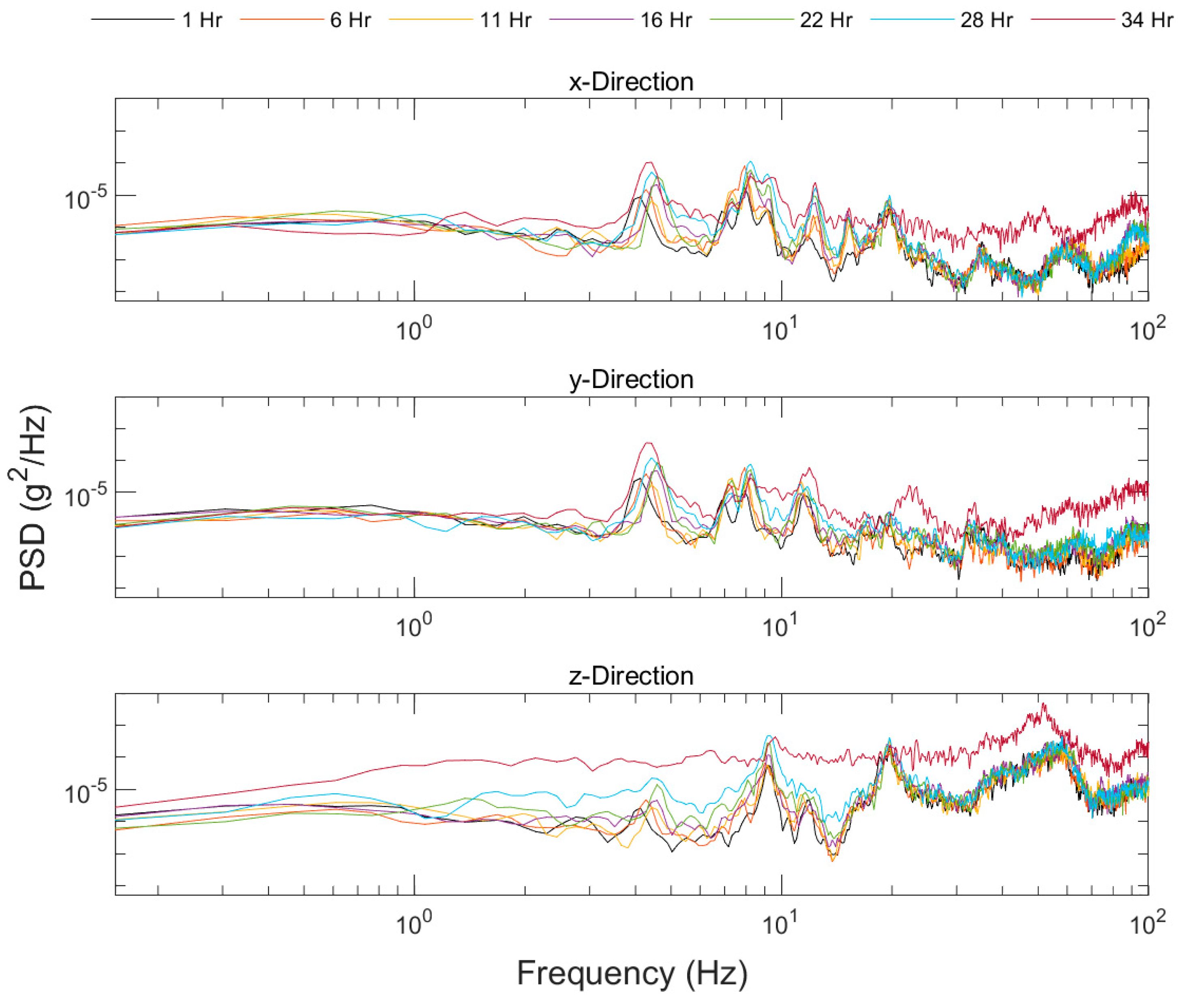
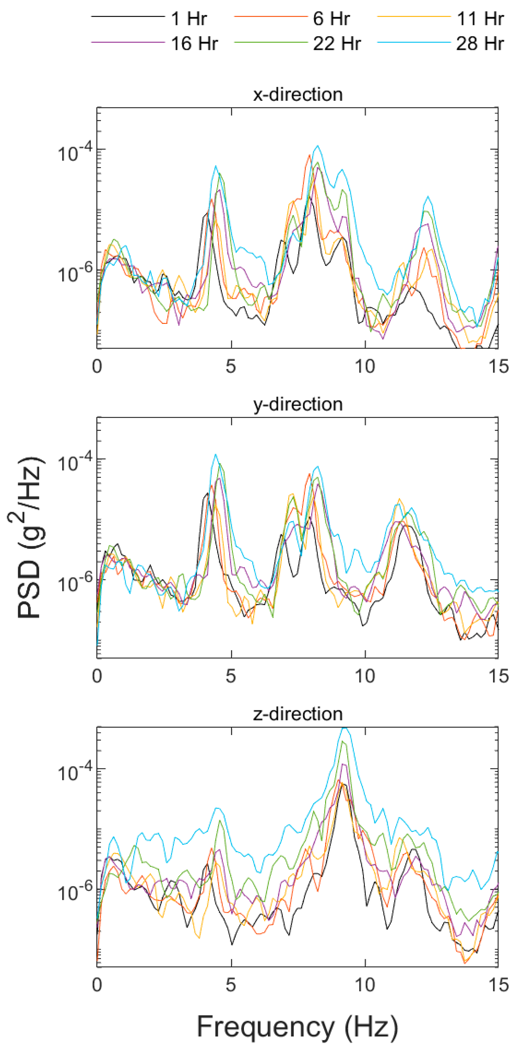
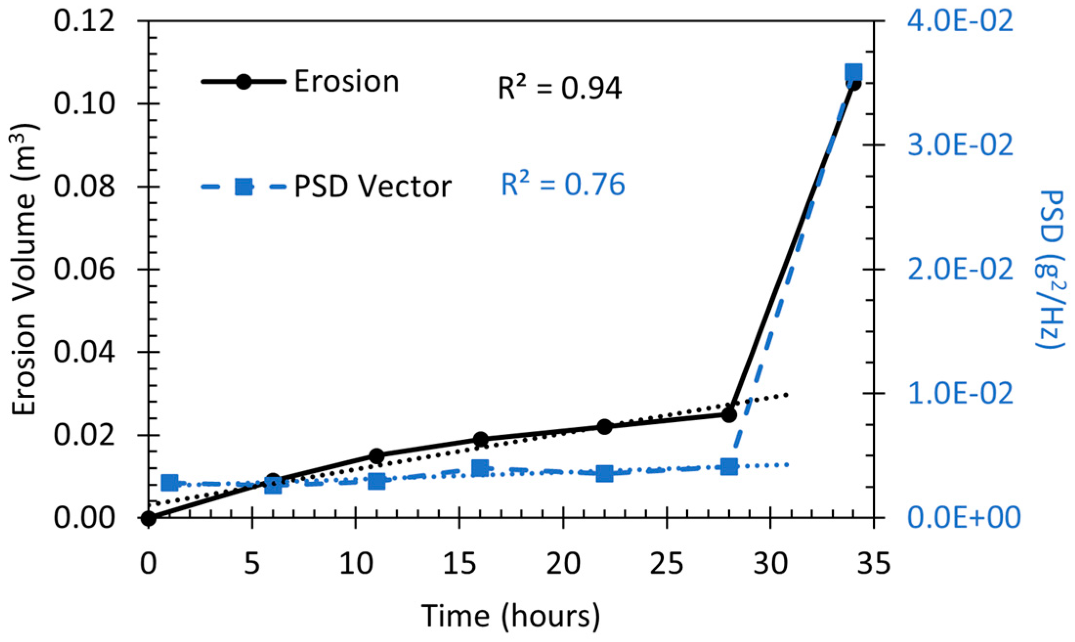
3.3. Erosion Vibration Response

Frequency analysis was conducted in 20 s intervals that aligned with the erosion scan data to determine the frequencies and PSDs that correlated to the erosion values. Figure 9 depicts the 20 s of acceleration data for the seven intervals in the x-, y-, and z-directions.

Figure 9 shows that the acceleration in the x- and y-directions is indistinguishable for the first six time intervals; only a major shift can be seen from the 28 to the 34 h intervals, referred to as the failure point. The z-direction appears to have higher acceleration amplitudes than the other two directions and has a major change in acceleration after the failure point occurs. The PSD analysis was performed for all seven intervals in all three directions and is depicted in Figure 10.

From Figure 10, it is apparent that the amplitude of the post-erosion dominant frequencies (i.e., 34 h) in the z-direction are significantly larger than those in the x- and y-directions. Since the PSD responses in the x- and y-directions are symmetric, a symmetric behavior between the responses can be seen in the x- and y-directions of Figure 10. Since the z-direction is perpendicular to the flow direction, additional forces due to the fluid weight and fluid hydrodynamic excitation cause higher vibration amplitude. The frequency response of the x- and y-directions shows that the first dominant frequency, around 4 Hz, does not exhibit much change, except for amplitude. A small frequency shift, 0.2 Hz, can be seen at the second dominant frequency, around 8 Hz, due to the erosion rate. Interestingly, the dominant frequency of each time span is seen with a pair of double frequencies around the dominant frequency, i.e., side bands. As the erosion rate increases, the side bands are less noticeable.

The dominant frequencies in all three directions appear to be in agreement with each other except for an increase in amplitude. An interesting observation in the x- and y-directions is that the first six time intervals are relatively on top of each other, with a major change in the 34 h time interval. However, the z-direction (Figure 10) has a different trend; the PSD amplitudes appear to increase in magnitude as the time interval increases. To further investigate this trend, a magnified region of the pre-erosion data from 0 to 15 Hz is shown in Figure 11.

Excluding the post-erosion data from Figure 10 and Figure 11 shows a clearer trend at the lower frequency range. All three directions show that the amplitude of the frequencies increases as time increases while the relative peak values remain the same. This trend is masked in Figure 10 due to the amplitude of the post-erosion vibrations. To quantify the amplitude for each pre-erosion time frame, the PSD was averaged in each direction, normalized to the value in time interval 1 h, and is shown in Figure 12. From Figure 12, there appears to be a positive association between the average PSD powers and time intervals in all three directions. However, there are some anomalies in the data that do not match with the general trend such as at the 6 h time interval for the x- and y-directions and the 22 h interval for the z-direction. Plotting the average PSD time intervals for each axis results in Figure 13. Note that the pre-erosion PSD powers follow a linear trend as indicated by their respective high coefficients of determination (R²).

4. Discussion

From the previous sections, soil erosion was quantified with respect to time and resulted in a linear relationship between erosion and time prior to the failure point. Vibrations caused by water being discharged over the soil were analyzed, and the average PSD powers for the x-, y-, and z-directions were determined. The PSD analysis shows that there is a linear relationship between the average power and time. To compare the PSD analysis with the erosion values, a vector sum formula was used to calculate the overall magnitude of the PSD power at each time interval from Figure 13, shown in Figure 14.

The erosion volume and PSD power spectra follow a similar linear trend until the failure point occurs. Since both dependent variables have similar responses, they are plotted against each other to show their relationship (Figure 15). Figure 15 shows that there is a positive relationship between the vibrational amplitudes in the soil and the resulting soil erosion.

Although there is a relationship between in situ vibrations and soil erosion, the coefficient of determination (R²) in Figure 15 is not as strong as the authors would like. Many variables can be credited to why the relationship between vibrations and erosion is not stronger. As discussed in Section 3.3, the PSD amplitudes at the 6 h time interval were higher than the trend. This can be attributed to the test methodology. The stopping and starting of the water could cause irregularities in the vibrational measurements. Another variable is the size of the test flume. The test flume consisted of 2.6 m² in surface area in which approximately 0.4 m³ of soil was used, which leads to ample opportunities for irregularities to occur such as uneven compaction, non-uniform soil, and variations in the moisture content. Furthermore, the quantity of accelerometers should be investigated to ensure vibrational measurements occur where sensors are placed. Erosion during this test occurred at the location of the accelerometer but based on the erosion scans (Figure 4) and the progression of the erosion, more accelerometers should have been placed throughout the test area to measure vibrations more accurately along the erosion pathway. As shown in the vibration data, the amplitudes were significantly higher after the failure point. This could be attributed to the fact that the sensor was exposed to the water discharge after the failure point (Figure 6). Further testing should alter the depth of the accelerometer(s) to determine if the vibrations can be measured under larger amounts of soil.

After testing was complete, soil analysis tests were performed, and it was found that the optimum moisture content of the clay was 13.0%. Therefore, the material was placed above the optimum moisture content. Moisture content, soil type, soil thickness, test area size and shape, and water velocity should all be investigated further to validate the relationship between soil vibrations and erosion.

Although the linear regression model has a relatively poor coefficient of determination (R²), there is evidence that surface soil erosion, or at least soil integrity, can be predicted by in situ vibrations, which is in agreement with [27,28,29,30], where acoustic emissions to predict internal soil erosion/seepage were used. For applications involving earthen dams, accelerometers can be installed during construction or rehabilitation and be used to autonomously monitor the integrity of the dam. If an overtopping event were to occur, then the accelerometers could have an automated program that alerts emergency officials if the dam is showing signs of a major erosion event. If the amplitude of the vibrations were to increase as flood conditions continued, then emergency response personnel could have valuable time to prepare and warn the public or perform alternative measures. From a theoretical point of view, using accelerometers to predicate soil erosion allows for model verification and future prediction using the dominant soil frequencies obtained from the vibration data analysis.

5. Conclusions

More than half of the USDA- and NRCS-sponsored earthen dams constructed under the USDA Small Watershed Program authority have surpassed their planned service life. Soil erosion has been shown to be an issue in earthen dam integrity due to its potential to occur without warning. The objective of this work was to test if soil erosion can be predicted using frequency vibrations from an in-situ accelerometer (i.e., acoustic emissions). A 0.61-by-4.27-m test flume was constructed and filled with 0.15 m of inorganic clay compacted above the optimum moisture content. A constant flow discharge of 0.07 m³/s was applied to the flume until complete failure of the test section occurred. 3D point scan images and in situ vibrations were collected during the test to correlate erosion and vibration frequency amplitudes. This work developed a methodology to quantify soil erosion with respect to time by analyzing induced vibrations using a PSD analysis. The sampling rate of the accelerometers was optimized to ensure accuracy while limiting collected data. The results indicated a linear relationship between erosion and time, vibration amplitudes and time, and ultimately a relationship between erosion and vibrational amplitudes. Future work will include the tested soil moisture content, soil type, soil thickness, test area size and shape, water velocity, quantity of accelerometers, and various measurement depths. Further research on the effect of soil properties on the dominant frequencies will be investigated to allow for better erosion prediction and model development.

References

1. Association of State Dam Safety Officials (ASDSO). ASDSO Incident Database Input Form. 2024. Available online: https://www.damsafety.org/content/asdso-incident-database-input-form (accessed on 5 February 2024).
2. Foster, M.; Fell, R.; Spannagle, M. The statistics of embankment dam failures and accidents. Can. Geotech. J. 2000, 37, 1000–1024. [Google Scholar] [CrossRef]
3. Costa, J.E. Floods from Dam Failures; US Geological Survey: Reston, VA, USA, 1985; Volume 85, No. 560. [Google Scholar] [CrossRef]
4. Caldwell, L. USDA Watershed Programs Facts and Figures: A Reservoir of Watershed Program Information; US Department of Agriculture Natural Resources Conservation Service (NRCS), Conservation Engineering Division: Washington, DC, USA, 2020. [Google Scholar]
5. Anderson, N.L.; Ismael, A.M.; Thitimakorn, T. Ground-penetrating radar: A tool for monitoring bridge scour. Environ. Eng. Geosci. 2007, 13, 1–10. [Google Scholar] [CrossRef]
6. Di Prinzio, M.; Bittelli, M.; Castellarin, A.; Pisa, P.R. Application of GPR to the monitoring of river embankments. J. Appl. Geophys. 2010, 71, 53–61. [Google Scholar] [CrossRef]
7. Anchuela, Ó.P.; Frongia, P.; Di Gregorio, F.; Sainz, A.C.; Juan, A.P. Internal characterization of embankment dams using ground penetrating radar (GPR) and thermographic analysis: A case study of the Medau Zirimilis Dam (Sardinia, Italy). Eng. Geol. 2018, 237, 129–139. [Google Scholar] [CrossRef]
8. Shin, S.; Park, S.; Kim, J.H. Time-lapse electrical resistivity tomography characterization for piping detection in earthen dam model of a sandbox. J. Appl. Geophys. 2019, 170, 103834. [Google Scholar] [CrossRef]
9. Guo, Y.; Cui, Y.A.; Xie, J.; Luo, Y.; Zhang, P.; Liu, H.; Liu, J. Seepage detection in earth-filled dam from self-potential and electrical resistivity tomography. Eng. Geol. 2022, 306, 106750. [Google Scholar] [CrossRef]
10. Sanuade, O.; Ismail, A. Geophysical and Geochemical Pilot Study to Characterize the Dam Foundation Rock and Source of Seepage in Part of Pensacola Dam in Oklahoma. Water 2023, 15, 4036. [Google Scholar] [CrossRef]
11. Marescot, L.; Monnet, R.; Chapellier, D. Resistivity and induced polarization surveys for slope instability studies in the Swiss Alps. Eng. Geol. 2008, 98, 18–28. [Google Scholar] [CrossRef]
12. Abdulsamad, F.; Revil, A.; Ahmed, A.S.; Coperey, A.; Karaoulis, M.; Nicaise, S.; Peyras, L. Induced polarization tomography applied to the detection and the monitoring of leaks in embankments. Eng. Geol. 2019, 254, 89–101. [Google Scholar] [CrossRef]
13. Sazal, Z.; Sanuade, O.; Ismail, A. Geophysical characterization of the Carl Blackwell earth-fill dam: Stillwater, Oklahoma, USA. Pure Appl. Geophys. 2022, 179, 2853–2867. [Google Scholar] [CrossRef]
14. Wise, J.; Hunt, S.; Al Dushaishi, M. Prediction of earth dam seepage using a transient thermal finite element model. Water 2023, 15, 1423. [Google Scholar] [CrossRef]
15. Fadaei-Kermani, E.; Shojaee, S.; Memarzadeh, R.; Barani, G.A. Numerical simulation of seepage problem in porous media. Appl. Water Sci. 2019, 9, 79. [Google Scholar] [CrossRef]
16. Aniskin, N.A.; Antonov, A.S. Using mathematical models to study the seepage conditions at the bases of tall dams. Power Technol. Eng. 2017, 50, 580–584. [Google Scholar] [CrossRef]
17. Alekseevich, A.N.; Sergeevich, A.A. Numerical modelling of tailings dam thermal-seepage regime considering phase transitions. Model. Simul. Eng. 2017, 2017, 7245413. [Google Scholar] [CrossRef]
18. Dardanelli, G.; Pipitone, C. Hydraulic models and finite elements for monitoring of an earth dam, by using GNSS techniques. Period. Polytech. Civ. Eng. 2017, 61, 421–433. [Google Scholar] [CrossRef]
19. Zhou, W.; Li, S.; Zhou, Z.; Chang, X. InSAR observation and numerical modeling of the earth-dam displacement of Shuibuya Dam (China). Remote Sens. 2016, 8, 877. [Google Scholar] [CrossRef]
20. Gordan, B.; Adnan, A.; Aida, M.A. Soil saturated simulation in embankment during strong earthquake by effect of elasticity modulus. Model. Simul. Eng. 2014, 2014, 191460. [Google Scholar] [CrossRef]
21. Kheiry, M.; Kalateh, F. Uncertainty Quantification of Steady-State Seepage Through Earth-fill Dams by Random Finite Element Method and Multivariate Adaptive Regression Splines. J. Hydraul. Struct. 2023, 9, 48–74. [Google Scholar] [CrossRef]
22. Azimi Sardari, M.R.; Bazrafshan, O.; Panagopoulos, T.; Sardooi, E.R. Modeling the impact of climate change and land use change scenarios on soil erosion at the Minab Dam Watershed. Sustainability 2019, 11, 3353. [Google Scholar] [CrossRef]
23. Kalateh, F.; Kheiry, M. A Review of Stochastic Analysis of the Seepage Through Earth Dams with a Focus on the Application of Monte Carlo Simulation. Arch. Comput. Methods Eng. 2024, 31, 47–72. [Google Scholar] [CrossRef]
24. Vrieling, A. Satellite remote sensing for water erosion assessment: A review. Catena 2006, 65, 2–18. [Google Scholar] [CrossRef]
25. Nasategay, F.F.U. Detection and Monitoring of Tailings Dam Surface Erosion Using UAV and Machine Learning. Ph.D. Thesis, University of Nevada, Reno, NV, USA, 2020. [Google Scholar]
26. Slingerland, N.; Sommerville, A.; O’Leary, D.; Beier, N.A. Identification and quantification of erosion on a sand tailings dam. Geosystem Eng. 2020, 23, 131–145. [Google Scholar] [CrossRef]
27. Rinehart, R.V.; Parekh, M.L.; Rittgers, J.B.; Mooney, M.A.; Revil, A. Preliminary implementation of geophysical techniques to monitor embankment dam filter cracking at the laboratory scale. In Proceedings of the ICSE6, Paris, France, 27–31 August 2012. ICSE6-103. [Google Scholar]
28. Fisher, W.D.; Camp, T.K.; Krzhizhanovskaya, V.V. Anomaly detection in earth dam and levee passive seismic data using support vector machines and automatic feature selection. J. Comput. Sci. 2017, 20, 143–153. [Google Scholar] [CrossRef]
29. Talwani, P.; Acree, S. Pore pressure diffusion and the mechanism of reservoir-induced seismicity. In Earthquake Prediction; Birkhäuser: Basel, Switzerland, 1985; pp. 947–965. [Google Scholar] [CrossRef]
30. Talwani, P. Seismotectonics of the Koyna-Warna area, India. In Seismicity Associated with Mines, Reservoirs and Fluid Injections; Birkhäuser: Basel, Switzerland, 1998; pp. 511–550. [Google Scholar] [CrossRef]
31. Larsen, D.C. Water Measurement; Issue 552 of Bulletin; University of Idaho, College of Agriculture: Moscow, ID, USA, 1976. [Google Scholar]
Figure 1. Schematic of the erosion test flume.
Water 16 01009 g001
Figure 2. Raw discharge data and acceleration data in the three directions with respect to relative time.
Water 16 01009 g002
Figure 3. (a) Campbell Scientific CS475A water radar sensor used for autonomous discharge measurement. (b) Gravity head tank that provided the water discharge for the test. (c) Erosion of the soil at the inlet of the test flume.
Water 16 01009 g003
Figure 4. 3D point cloud scans depicting the progression of soil erosion during testing. Note that the orange color represents high spots, and the dark blue represents voids (i.e., erosion).
Water 16 01009 g004
Figure 5. Quantified soil erosion values throughout testing with a trendline (dashed line) showing the linear relationship between erosion and time before the failure point.
Water 16 01009 g005
Figure 6. (a) Final scan of the test flume showing the eroded soil. This erosion event is referenced as the failure point of the test. (b) Zoomed in region showing the exposed accelerometer.
Water 16 01009 g006
Figure 7. 20 s acceleration data in all three directions for the range of sampling rates.
Water 16 01009 g007
Figure 8. PSD response at the 1 h time interval for all three directions with different sampling rates.
Water 16 01009 g008
Figure 9. Acceleration data for the seven time intervals in the x-, y-, and z-directions.
Water 16 01009 g009
Figure 10. PSD versus frequency analysis for the x-, y-, and z-directions.
Water 16 01009 g010
Figure 11. Magnified pre-erosion PSD versus frequency data for the x-, y-, and z-directions.
Water 16 01009 g011
Figure 12. Averaged and normalized PSD power for each direction from 0 to 100 Hz.
Water 16 01009 g012
Figure 13. PSD power amplitudes versus time for all three axes. The pre-erosion amplitudes follow a linear trend as indicated by the dotted trendlines and their respective coefficients of determination.
Water 16 01009 g013
Figure 14. PSD power and erosion of the test with respect to time.
Water 16 01009 g014
Figure 15. PSD power spectra versus erosion volume values and their resulting linear relationship.
Water 16 01009 g015