Stress Prediction Model of Super-High Arch Dams during Their Initial Operation Stages

Abstract

It is of great significance to identify the spatiotemporal stress distribution characteristics to ensure the safety of a super-high arch dam during the initial operation stage. Taking the 285.5 m-high Xiluodu Dam as an example, the spatiotemporal distribution characteristics were analyzed based on the five-year observation data after impoundment. Statistical and boosted-regression-tree-based prediction models for the dam stress were established. The boosted-regression-tree-based prediction model is more accurate than the statistical model. The monitoring indicators for the measuring points of focused locations were determined using the confidence interval estimation method. The results show that the dam was in a compression state, and the arching effect was obvious. The arch direction compressive stress gradually increased and stabilized, and the maximum appeared in the middle of the upstream face of the crown cantilever monolith. For the crown cantilever, the cantilever direction stress at the dam heel was significantly affected by the interior temperature recovery, and the arch direction stress in the middle of the upstream face was significantly affected by the reservoir water level. The measuring points of the focused locations with reliable observation data can be selected as a monitoring index to guide the initial operation.

1. Introduction

A number of super-high arch dams with a height of over 200 m have been built in China [1,2]. These super-high arch dams have complex structures and are mostly constructed in high valleys, and their initial operation environments are complicated [3]. During the initial operation stage, the reservoir water level (RWL) fluctuates greatly, and dam stress and strain continue to adjust. After arch sealing, there would be a temperature rise inside the dam, which would increase the compressive stress of the dam heel and increase the risk of cracking on the dam’s downstream surface [4,5]. Affected by filling, the vertical stratification of reservoir water temperature (RWT) would also occur in front of a super-high arch dam during the initial operation stage [6,7]. The difference between the actual and designed RWT also affects thermal stress. In addition, valley deformation further affects the dam stress distribution [3]. Due to the influence of the complex environment and load factors, the actual working behavior of a super-high arch dam during the initial operation stage is often inconsistent with the designed state. Ensuring the safety of super-high arch dams during this stage involves many challenges [8].

For concrete dams, overstressing is the dominant factor leading to cracks, and it is also an important indicator affecting dam safety and overall stability [9,10,11,12,13]. Therefore, stress is commonly considered as a control indicator in design. Measured stress–strain can directly reflect the stress distribution characteristics and working behavior of a concrete dam. Considering the particularity of the initial operation stage, the stress and distribution characteristics are the important issues that managers focus on. However, as endoscopic instruments, strain gauge groups are susceptible to construction disturbances and faults in the automated acquisition systems. In addition, it is also necessary to embed the strain gauge group and the stress-free gauge at the same time to obtain the actual stress. The elastic modulus and creep degree should also be obtained from the concrete test. Then, the measured values of the strain gauge group and stress-free strain meter can be converted into actual stress. The complexity of the conversion process and errors in the observation process have made research into stress prediction models very limited compared to that concerned with deformation [14,15,16].

Due to their extreme importance, super-high arch dams make greater demands for strength and stability of the dam foundation and require stricter safety control than lower arch dams. In addition, super-high arch dams present greater challenges in terms of issues such as crack prevention and temperature and crack control during the construction and initial operation stages [1]. Focusing on the structural control requirement of a number of 300 m-level super-high arch dams, such as Xiaowan, Xiluodu, and Jinping I, a lot of research has been carried out on the actual working behavior of super-high arch dams, utilizing numerical investigations and physical tests. Zhang et al. [17] discussed the effects of temperature, self-weight exaction way, and water loading on structure response. Lin et al. [18] identified and compared the dam stress characteristics and deformation distribution of the Xiaowan Dam based on four 3D geomechanical model tests. Luo et al. [19] studied the effect of the first filling process on the overall stability of the Xiluodu Dam via field monitoring and numerical modeling methods. Wu et al. [2] used monitoring data analysis and numerical calculation to analyze the working behavior of the Jinping-I Dam during the initial impoundment. Tao et al. [8] carried out a geomechanical model test to study the nonlinear deformation and failure mechanism of the Mengdigou Dam. Liu et al. [9] mentioned that there are four actual factors—material, structure, load, and process—that need to be considered during stress computation. The above studies revealed the actual stress characteristics and working behavior of super-high arch dams to a certain extent.

However, few comprehensive analyses of stress have been conducted for a super-high arch dam during the initial operation stage based on field monitoring due to the aforementioned difficulties. The monitoring of stress and strain permits us to grasp the spatiotemporal distribution characteristics of the stress and allows for early detection of abnormal behavior. Taking the Xiluodu Dam as an example, the deformation and stress change laws reflected in the monitoring data after impounding are not completely consistent with the design. The dam deformed upstream after the first filling. Though the reservoir was filled to the normal RWL, the dam heel was still under compression. In addition, the upper valley width was in a state of contraction with the RWL rise [20,21,22]. Therefore, the spatiotemporal distribution characteristics of the Xiluodu Dam during the initial operation stage were comprehensively analyzed in this paper.

This paper is organized as follows: Section 2 describes the calculation process of measured stress of concrete dam, as well as the safety monitoring models for concrete stress and strain. Section 3 briefly introduces the Xiluodu arch dam, the initial operation process, and the stress monitoring equipment. Based on the observation data, the stress change process and the spatiotemporal distribution characteristics during the initial operation stage are analyzed in Section 4. On this basis, statistical and prediction models of stresses at key measuring points are built, the influence mechanism of the dominant predictors of stress is obtained, and monitoring indicators are determined in Section 5. The prediction model established in this paper is more accurate than the traditional models, and the results were discussed in detail based on actual loads and environmental conditions. The research in this paper is of great significance in guiding the initial operation of super-high arch dams.

2. Calculation and Constructing Statistical Model for Stress of Super-High Arch Dams

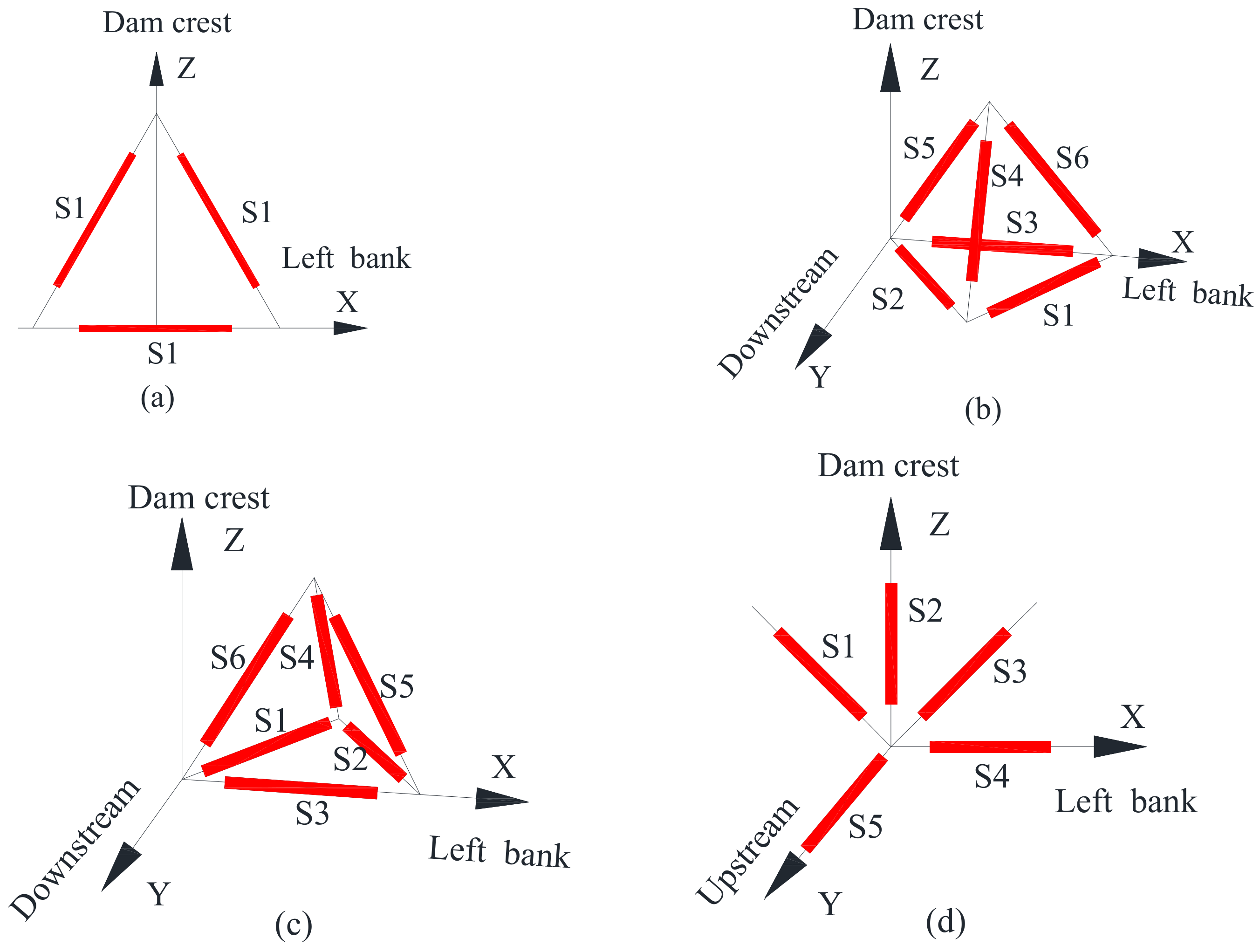
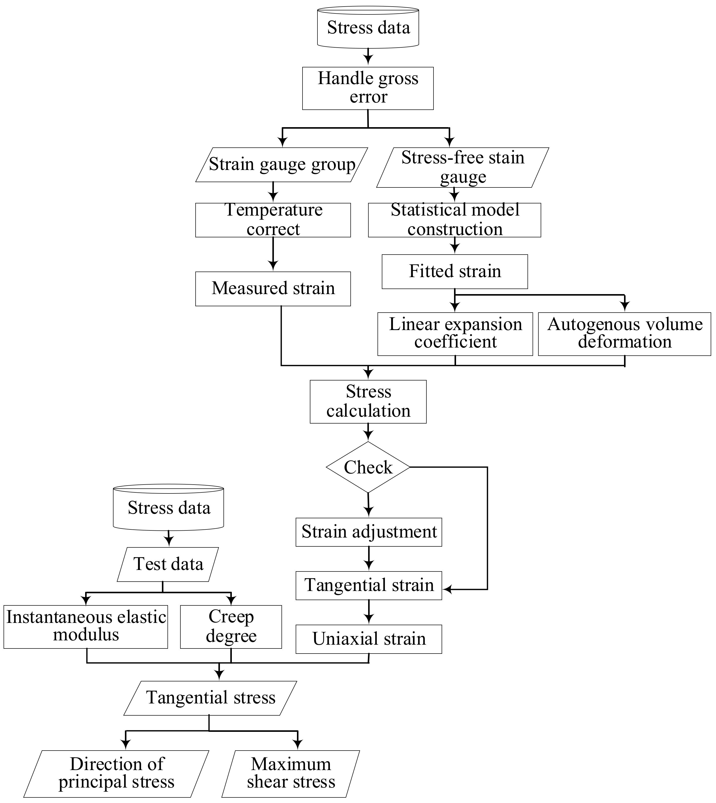
2.1. Calculation of Measured Stresses of Concrete Dams

The total strain at a point in a concrete structure consists of two components [21]. One component is the strain due to loads and internal restraints. The other component is caused the temperature change, cement hydration, and hardening process, which is called the stress-free strain. Therefore, it is necessary to deduct the stress-free strain from the total strain when analyzing the measured stress. In order to obtain the autogenous volume deformation, at least one stress-free gauge should be buried near a strain gauge group.

Common strain gauge groups include three-, five-, and six-direction types (Figure 1) [16]. The stress should be calculated using the measured data of the strain gauge group. According to the spatial relationship of strain gauges in a group, the three-direction normal strain at a measuring point can be calculated. In order to improve the calculation accuracy and eliminate gross errors, it is necessary to check the reliability of the measured data. Strain balance means that two strain gauges arranged vertically at 90° in the same plane should satisfy the first strain invariant; that is, S₁ + S₃ = S₂ + S₄. According to this principle, it is necessary to check the strain unbalance to eliminate the error caused by the installation and buried quality for the five-direction strain gauge group. For the six- and the three-direction strain gauge groups, the unbalance check cannot be performed, and the stress calculation cannot be performed if one-direction strain gauge fails.

The relationship between the normal strain ε_i along any direction in space and the strain component in the local coordinate system is

$${\epsilon }_i=l_{2i}{\epsilon }_x+m_{2i}{\epsilon }_y+n_{2i}{\epsilon }_z+l_i{m}_i{\gamma }_{xy}++m_i{n}_i{\gamma }_{yz}+n_i{l}_i{\gamma }_{zx},$$

(1)

where l_i, m_i, and n_i represent the cosine of the corresponding direction of the strain e_i; O_zxy represents the local coordinate system at the measuring point; x, y, and z represent the arch direction (pointing to the left bank is positive), the radial direction, and the cantilever direction; and strain is positive for tension and negative for compression.

Taking the six-direction strain gauge group as an example, the linear equation of six unknowns is established by Equation (1), and the equation is solved by

$$\left\{\begin{array}{c}\begin{array}{c}{\epsilon }_x={\epsilon }_3\\ {\epsilon }_y=\left(2{\epsilon }_1+2{\epsilon }_2-{\epsilon }_3\right)/3\\ {\epsilon }_z=\left(-{\epsilon }_1-{\epsilon }_2-{\epsilon }_3+3{\epsilon }_4+{3\epsilon }_5+{3\epsilon }_6\right)/6\end{array}\\ \begin{array}{c}{\gamma }_{xy}=2\left({\epsilon }_1-{\epsilon }_2\right)/\sqrt{3}\\ {\gamma }_{yz}=\sqrt{2}\left({\epsilon }_1+{\epsilon }_2-2{\epsilon }_3-6{\epsilon }_4+{3\epsilon }_5+{3\epsilon }_6\right)/\sqrt{6}\\ {\gamma }_{zx}=\left(-{\epsilon }_1+{\epsilon }_2-{3\epsilon }_5+{3\epsilon }_6\right)/\sqrt{6}\end{array}\end{array}\right.,$$

(2)

where ε₁, ε₂, ε₃, ε₄, ε₅, and ε₆ represent the measured strain value of each strain gauge.

The stress and strain relationship under sustained load is calculated as follows:

$${\sigma }_{x,y,z}=E^{\prime }\left(\tau ,t\right){{\sigma }^{\prime }}_{x,y,z},$$

(3)

$$E^{\prime }\left(\tau ,t\right)=1/\left[\left(1/E\left(t\right)\right)+C\left(\tau ,t\right)\right],$$

(4)

$${{\epsilon }^{\prime }}_{x,y,z}=\frac{1}{\left(1+\mu \right)\left(1-2\mu \right)}\left[\left(1-\mu \right){\epsilon }_{x,y,z}+\mu \left({\epsilon }_{y,z,x}+{\epsilon }_{z,x,y}\right)\right],$$

(5)

where ${\sigma }_{x,y,z}$ is the stress in the x, y, and z directions, MPa; ${{\epsilon }^{\prime }}_{x,y,z}$ is uniaxial strain along the x, y, and z directions, ×10⁻⁶; $E^{\prime }\left(\tau ,t\right)$ is the continuous elastic modulus of concrete, ×10⁴ MPa; $E\left(t\right)$ is the instantaneous elastic modulus of concrete, ×10⁴ MPa; and $C\left(\tau ,t\right)$ is the creep deformation, ×10⁻⁶/MPa, which be fitted from concrete tests.

For the five-directional strain gauge group, a strain imbalance check is required. When one of the four strain gauges arranged in the same plane fails, a stress calculation can still be performed based on plane stress or plane strain. If more than one strain gauge fails, stress calculation can no longer be performed. After the strain matrix at the measuring point is obtained, the stress-free deformation is deducted, and then the creep stress of the concrete can be calculated according to the deformation method, which can directly use the experiment data of the creep degree to calculate the total deformation of uniaxial strain. In order to calculate the stress, the elastic modulus and the concrete creep test data should be fitted and calculated by fitting the experiment data. According to the test data, the creep curve of the concrete can be fitted. Under the condition of measured strain and creep test data, the deformation method can be used to calculate the stress along all directions [16]. Among them, the three-direction and six-direction strain gauge groups are not balanced. The flow of stress calculation is shown in Figure 2.

2.2. Prediction Models for Concrete Stress and Strain

2.2.1. Statistical Model of Stress-Free Strain

The stress-free deformation of concrete includes three components: temperature deformation, autogenous volume deformation, and humidity deformation [23,24]. Measuring stress-free strain is undertaken in order to understand the linear expansion coefficient and autogenous volume deformation of the dam concrete. The variation law of the stress-free strain of concrete can be understood through the regression analysis.

The statistical model of the stress-free strain is given by [25]

$${\epsilon }_0=a_0+a_{1}T+a_2\theta +a_3\mathrm{l}\mathrm{n}\left(1+\theta \right)+a_4(e^{k\theta }-1),$$

(6)

where T is the difference between the current temperature and the temperature of the starting day of the stress-free measuring point; θ = 0.01 t, where t is the number of days from the observation date to the initial measurement date; a₀, a₁, a₂, a₃, and a₄ are the regression coefficients; and k is a constant, which is taken as 0.01 here.

Here, the influence of humidity change is ignored. When Equation (6) is solved, the obtained a₁ is the estimated value of the linear expansion coefficient of the dam concrete. The rest, except the temperature component $a_{1}T$, is the time-dependent effect (TDE) component, that is, the autogenous volume deformation.

2.2.2. Statistical Model of Measured Stress

There are several factors that affect the stress of super-high arch dams, mainly related to hydrostatic pressure, the thermal component, and operation time. The TDE component is significant during the initial operation stage and tends to be stable in the later long-term operation stage. Thus, this component is expressed as the logarithm of time or its combination with the linear function of time. The expression of the thermal component can be divided into three types: the measured temperature, the equivalent temperature, and the periodic term [6,7,26]. Here, considering that the temperature field of the dam is not stable, the periodic term should not be adopted. Generally, a number of RWT thermometers at different elevations would be arranged on the upstream face of a newly built super-high arch dam. At the same time, a large number of strain gauge groups would be buried inside the dam, and the buried thermometers can also obtain the interior concrete temperature. Therefore, the measured temperature is selected as the expression of the thermal component for the super-high arch dam during the initial operation stage. The corresponding expression of the statistical model for concrete stress (hydrostatic pressure–thermal–time, HTT) is expressed as [27]

$$\sigma ={\displaystyle \sum _{i=1}^3{a}_i\left(H^i-H_0^i\right)}+{\displaystyle \sum _{i=1}^m{b}_i{T}_i}+c_1\left(\theta -{\theta }_0\right)+c_2\left(\ln \theta -\ln {\theta }_0\right)+d,$$

(7)

where σ is the stress; H and H₀ represent the RWL on the observation day and the initial observation day; T_i denotes the measured temperatures from the RWT thermometers and strain gauge groups near the measuring point; m is the number of selected thermometers; θ = 0.01 t, where t is the number of days from the observation day to the initial observation day; a, b, and c are coefficients; and d is a constant.

2.2.3. Boosted-Regression-Tree-Based Model for Measured Stress

Regression tree and gradient boosting are integrated in the boosted regression tree (BRT). Regression trees are simple models that fit a response variable to predictor variables by partitioning the feature space using a series of partition rules, e.g., binary split, to identify regions in the data which have the most consistent responses to predictors. A constant is then fitted to each region (e.g., mean response for observations in a particular region, in a regression problem). Gradient boosting, on the other hand, combines the output of weak learners (regression trees) to produce a more powerful and improved predictive performance. Therefore, the final BRT model would be a combination of several individual regression trees fitted in a forward stage-wise manner [7].

BRT can be applied to a typical predictive learning system consisting of a set of predictor variables X = {x₁, …, x_n} and a response variable y. For example, using a training sample {y_i, X_i}, i = 1, …, N of known y and X values, and we wish to find a function $\hat{f}\left(X\right)$ that maps X to y such that it minimizes the expected value of a specified loss function $\psi \left(y,f\right)$ over the joint distribution of all the values of (y, X):

$$\hat{f}\left(\mathrm{X}\right)=\arg \underset{f\left(\mathrm{X}\right)}{\min }{E}_{y,\mathrm{X}}\psi \left(y,f\left(\mathrm{X}\right)\right)=\arg \underset{f\left(\mathrm{X}\right)}{\min }{E}_{\mathrm{X}}\left[E_{y|\mathrm{X}}\psi \left(y,f\left(\mathrm{X}\right)\right)|\mathrm{X}\right].$$

(8)

If we initialize $\hat{f}\left(\mathrm{X}\right)$ to be a constant, $\hat{f}\left(\mathrm{X}\right)=\arg \underset{\rho }{\min }{\displaystyle {\sum }_{i=1}^N\psi \left(y_i,\rho \right)}$. For t in 1, …, T, we compute the negative gradient as the working response:

$$z_i=-\frac{\partial }{\partial f\left({\mathrm{X}}_i\right)}\psi \left(y_i,f\left({\mathrm{X}}_i\right)\right)|{ }_{\hat{f}\left({\mathrm{X}}_i\right)=f\left({\mathrm{X}}_i\right)}.$$

(9)

We fit a regression model, g(X), predicting z_i from the covariates X_i, and choose a gradient descent step size as

$$\rho =\arg \underset{\rho }{\min }{\displaystyle \sum _{i=1}^N\psi \left(y_i,\hat{f}\left({\mathrm{X}}_i\right)+\rho g\left({\mathrm{X}}_i\right)\right)}.$$

(10)

We update the estimate of f(X) as

$$\hat{f}\left(\mathrm{X}\right)\leftarrow \hat{f}\left(\mathrm{X}\right)|+\rho g\left(\mathrm{X}\right).$$

(11)

f(X) can be estimated as

$$\hat{f}\left(\mathrm{X}\right)=\arg \underset{f\left(\mathrm{X}\right)}{\min }{E}_{\mathrm{X}}\left[E_{y|\mathrm{X}}\psi \left(y,f\left(\mathrm{X}\right)\right)|\mathrm{X}\right].$$

(12)

Parametric regression models assume that f(X) is a function with a finite number of parameters, $\beta$, and estimates them by selecting those values that minimize a loss function (e.g., squared error loss) over a training sample of N observations on (y, X) pairs as

$$\hat{\beta }=\arg \underset{\beta }{\min }{\displaystyle \sum _{i=1}^N\psi \left(y_i,f\left({\mathrm{X}}_i;\beta \right)\right)}.$$

(13)

When we wish to estimate f(X) non-parametrically, the task becomes more difficult. Again, we can modify the estimate of f(X) by adding a new function f(X) in a greedy fashion. Letting f_i = f(X_i), we see that we want to decrease the N dimensional function:

$$J\left(\mathrm{f}\right)={\displaystyle \sum _{i=1}^N\psi \left(y_i,f\left({\mathrm{X}}_i\right)\right)}={\displaystyle \sum _{i=1}^N\psi \left(y_i,F_i\right)}$$

(14)

The negative gradient of J(f) indicates the direction of the greatest local decrease in J(f). Gradient descent would then have us modify f as

$$\hat{\mathrm{f}}\leftarrow \hat{\mathrm{f}}-\rho \nabla J\left(\mathrm{f}\right)$$

(15)

where ρ is the size of the step along the direction of greatest descent.

There are various ways to extend and improve upon the basic framework. In particular, by controlling the optimization speed or learning rate, introducing low variance regression methods, and applying ideas from robust regression, we can produce non-parametric regression procedures with many desirable properties. As a by-product, some of these modifications lead directly into implementations for learning from massive datasets. All these methods take advantage of the general form of boosting.

$$\hat{f}\left(\mathrm{X}\right)\leftarrow \hat{f}\left(\mathrm{X}\right)+E\left(z\left(y,\hat{f}\left(\mathrm{X}\right)\right)|\mathrm{X}\right)$$

(16)

In the update step of any boosting algorithm, we can introduce a learning rate to dampen the proposed move:

$$\hat{f}\left(\mathrm{X}\right)\leftarrow \hat{f}\left(\mathrm{X}\right)+\lambda E\left(z\left(y,\hat{f}\left(\mathrm{X}\right)\right)|\mathrm{X}\right)$$

(17)

By multiplying the gradient step by λ as in Equation (17), we have control over the rate at which the boosting algorithm descends the error surface. When λ = 1, we return to performing full gradient steps.

The greatest issue BRT models struggle with is the choice of the iteration number T and learning rate λ. The optimal iteration number T and the learning rate λ depend on each other. Smaller λ almost gives improved predictive performance. Performance is best when λ is as small as possible; that is, setting λ = 0.001 would almost certainly result in a model with better out-of-sample predictive performance.

Cross-validation is becoming increasingly common for selecting the optimal setting. The iteration number T is selected via cross-validation. Ten-fold cross-validation was applied to determine the optimal number of trees in the final ensemble with λ= 0.001 and T = 10,000.

Variable selection in BRT is achieved by largely ignoring non-informative predictors when fitting trees. Measures of relative influence quantify the importance of predictors, and irrelevant ones have minimal effect on prediction. However, unimportant variables can be dropped using methods analogous to backwards selection in regression. These are sometimes referred to as recursive feature elimination. This simplification process is run within a ten-fold cross-validation procedure, progressively simplifying the model fitted to each fold and using the average cross-validation error to decide how many variables can be removed from the original model without affecting predictive performance. Such simplification is most useful for small datasets where redundant predictors may degrade performance by increasing variance. In this way, the simplified BRT (SBRT) model can be established.

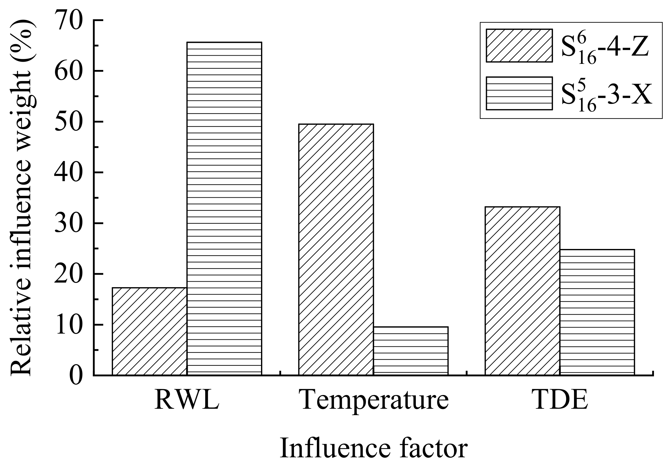
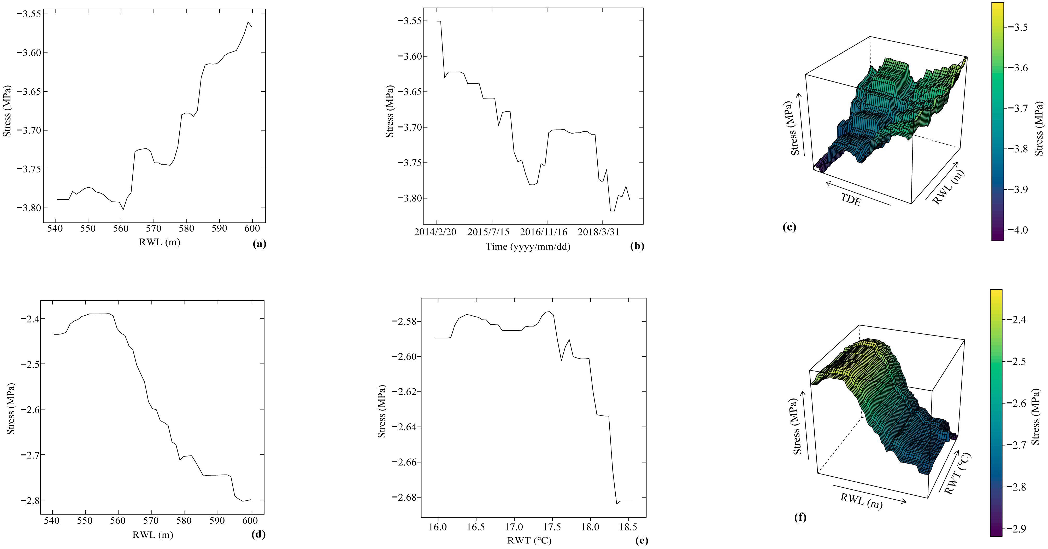
2.3. Partial-Dependence-Plot-Based Variable Influence Analysis

Partial dependence plot (PDP) is useful for knowledge discovery in large datasets [28]. PDP can be misleading in the presence of substantial interactions. Individual conditional expectation (ICE) plots are developed to overcome this issue. The PDP for a predictor of interest can be obtained by averaging the corresponding ICE curves.

If X is partitioned into an interest set, z_s, and its compliment, z_c = X/z_s, then the “partial dependence” of the response on z_s is defined as

$$f_s\left(z_s\right)=E_{z_c}\left[\hat{f}\left(z_s,z_c\right)\right]={\displaystyle \int \hat{f}\left(z_s,z_c\right)p_c\left(z_c\right)}d{z}_c$$

(18)

where $p_c\left(z_c\right)$ is the marginal probability density of z_c: $p_c\left(z_c\right)={\displaystyle \int p\left(x\right)}d{z}_s$. Equation (18) can be estimated from a set of training data by

$$f_s\left(z_s\right)=\frac{1}{n}{\displaystyle \sum _{i=1}^n\hat{f}\left(z_s,z_{i,c}\right)}$$

(19)

where z_i,c (i = 1, 2, …, n) are the values of z_c that occur in the training sample; that is, we average out the effects of all the other predictors in the model.

An alternative way to explain the effect of each predictor in the response is to identify the relative influence. For example, the approximate relative influence of a variable X_j for the tree-based methods is

$${\widehat{J}}_j^2={\displaystyle \sum _{x_j}{I}_t^2}$$

(20)

where $I_t^2$ is the empirical improvement by splitting X_j at that point.

The relative influence of each variable is proportional to the frequency with which they appear in the ensemble. The results are normalized so that they add up to 100. Based on this, the most influential variables can be identified for each output, and the results are interpreted in relation to dam behavior.

3. Project and Stress Monitoring Description

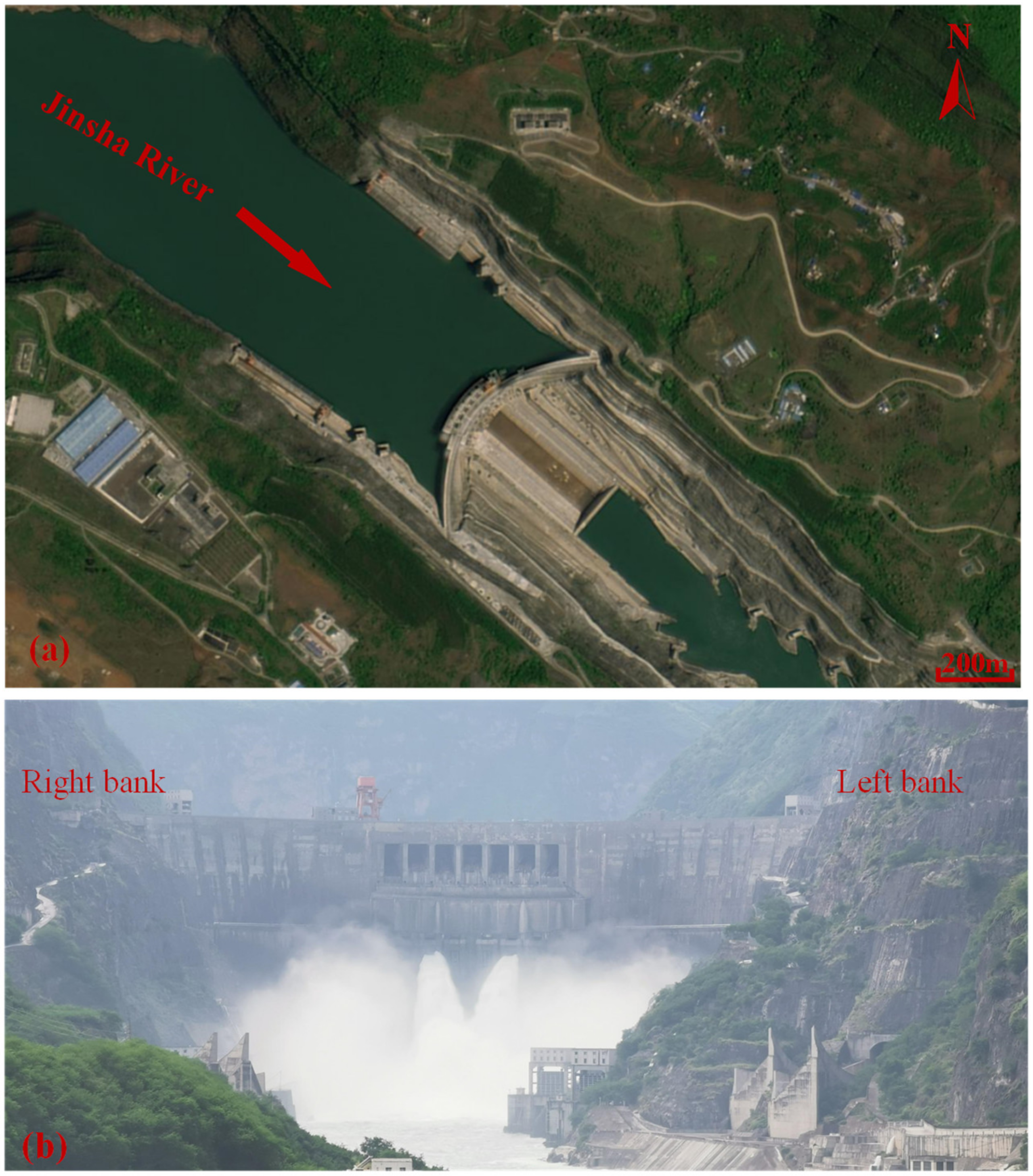
3.1. Project Description

The Xiluodu hydropower project (Figure 3) is located in the lower reaches of the Jinsha River in Southwest China. The dam is a double curvature arch dam, with a height of 285.8 m. As shown in Figure 4a, there are 31 monoliths planted across the river. The cross section of the dam is curved, 7 m wide at the crest and 60 m wide at the foundation. The dam site is U-shaped, embraced by steep side slopes. The normal, dead, and limited RWL are 600 m, 540 m, and 560 m, respectively. The RWL and the elevation (EL) are given in meters above sea level (m.a.s.l).

Concrete pouring of the dam began in March 2009. The lower gates of the deep outlets were closed on 4 May 2013. The concrete construction was completed in August 2013, and the joints were sealed in November 2013. The gates of surface outlets were installed and closed in April 2014. The project was fully completed as of June 2014.

The dam concrete is mainly divided into three zones: C₁₈₀40 in zone A, C₁₈₀35 in zone B, and C₁₈₀30 in zone C, as shown in Figure 4b. In addition, C₉₀42 concrete was used in the gate piers and orifices. The main indicators of dam concrete are listed in

Table 1. The main indicators of dam concrete.

Zone	A	B	C	Gate Pier and Orifice
Strength grade	C18040	C18035	C18030	C9042
Designed curing period (d)	180	180	180	90
Compressive strength (MPa)	≥40	≥35	≥30	≥42
Tensile strength (MPa)	≥3.2	≥3.0	≥2.8	≥3.4
Ultimate stretch (10−4)	≥1.00	≥0.95	≥0.90	≥1.00
Adiabatic temperature rise (°C)	≤28	≤27	≤26	≤29
autogenous volume deformation (10−6)	−20–10	−20–10	−20–10	−20–10
Concrete type	Normal	Normal	Normal	Normal
Concrete gradation	Two–four	Two–four	Two–four	Two, Three

. In the design stage, the deformation modulus of the dam concrete was assumed to be 24 GPa. Sensitivity analysis shows that when the deformation modulus of the dam changes in the range of 24–30 GPa, it has a certain influence on the displacement and the stress of the arch dam, but the influence magnitude is relatively small.

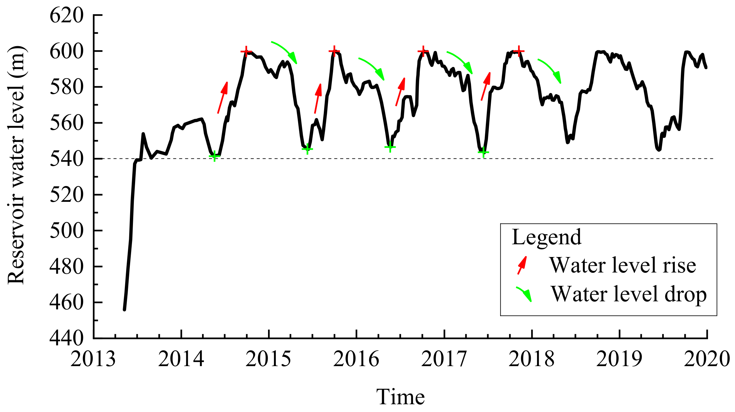
3.2. Initial Operation Process

Figure 5 depicts the change process of the RWL during the initial operation stage. This stage, covering the period from May 2013 until October 2018, is divided into four complete filling–discharging processes (i.e., loading and unloading processes). Specifically, the deep outlet gates were closed to start filling on 4 May 2013. Then, the RWL was gradually raised from EL 441.25 m and first filled to the normal RWL (EL 600 m) on 28 September 2014. The RWL began to drop on 18 March 2015 and dropped to EL 545.0 m on 13 June 2015. The next three periodic water filling–discharging processes are similar to the first process.

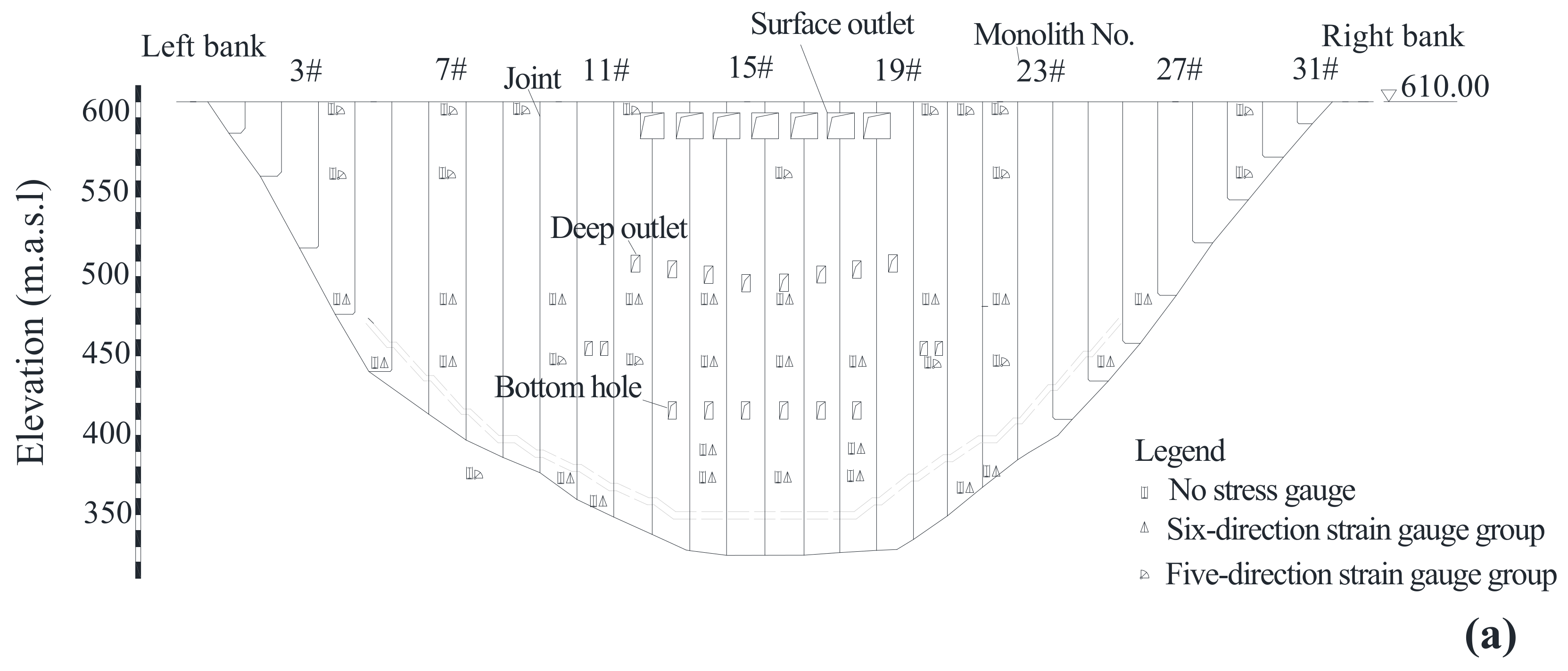
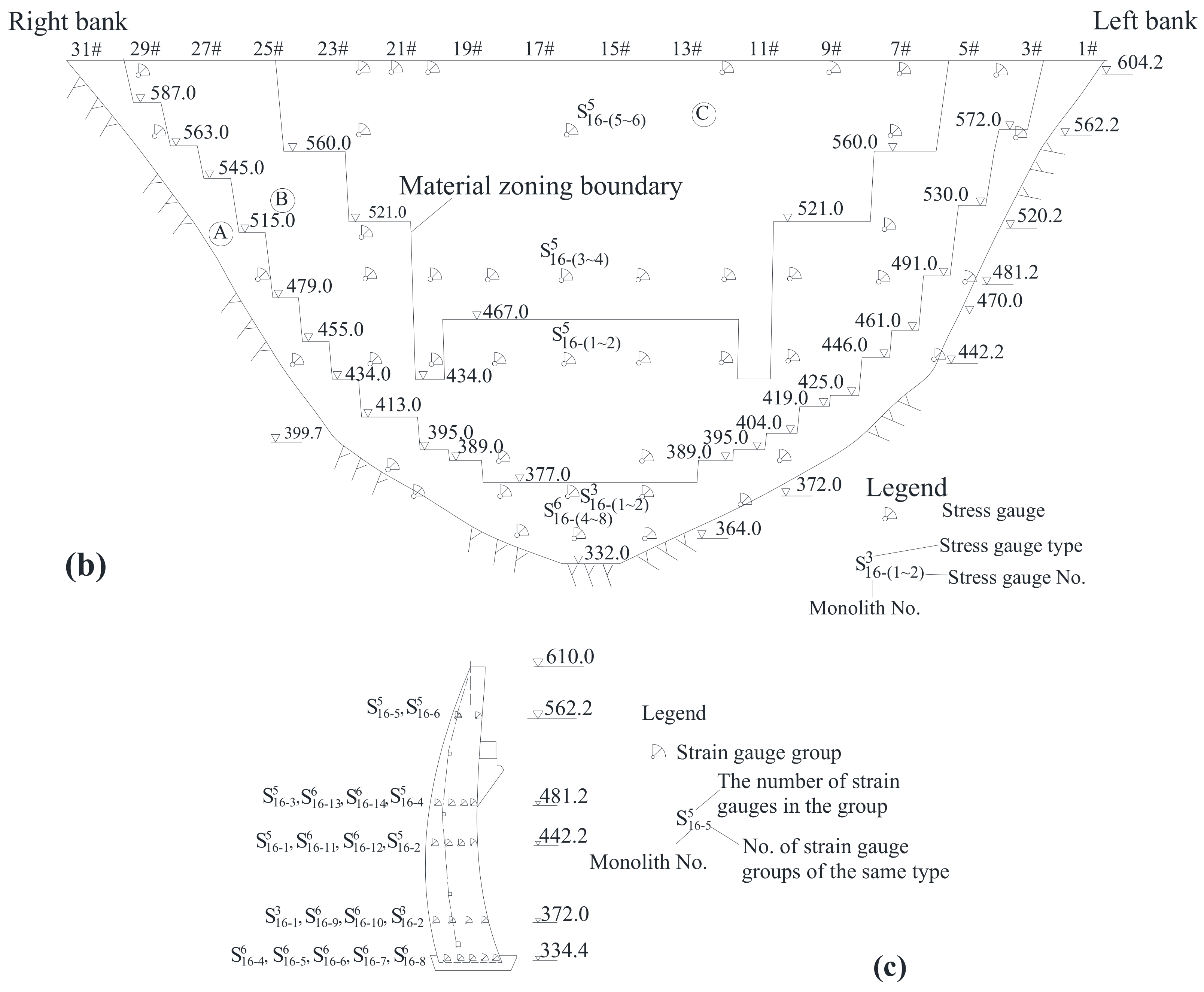
3.3. Stress Monitoring

The stress–strain monitoring equipment of the dam was mainly arranged in four arches and three cantilevers (Figure 4b). The four arches are EL 334.0 m, 442.2 m, 481.2 m, and 604.0 m, and the three cantilevers are monoliths 7, 16, and 22. Among them, the arrangement of the strain gauge groups of monolith 16 (the crown cantilever) is shown in Figure 4c. At the same elevation, the strain gauge groups were arranged in accordance with the principle of dispersed arrangement. This allows for the monitoring of the stress distribution from upstream to downstream. The upstream and downstream measuring points are, respectively, 4 m and 3 m away from the corresponding surfaces, and the remaining measuring points were located at equal intervals between the above two points. In addition, the measuring point of the downstream sticking angle area of the low elevation foundation is 4 m away from the boundary. The supporting stress-free gauge is within 2 m of the corresponding strain gauge group.

According to the corresponding stress states of different locations, the strain gauge groups were arranged in three-, five-, and six- directions (Figure 1). A total of 145 strain gauge groups were arranged, and the numbers of the three strain gauge groups were 10, 66, and 69, respectively. The arrangement of the six-direction strain gauge group is divided into types a and b. Type a was buried in the upstream side, and type b was buried in the downstream side. The six-direction strain gauge group was arranged below EL 481.2 m to monitor the spatial stress. The five-direction strain gauge groups were mainly arranged on the upstream and the downstream sides of the dam and were used to calculate the spatial normal stress and the plane principal stress of plane zx. S^M_N-L-X represents the L-th measuring point of M-direction of monolith N; X represents the normal stress direction;and X, Y, and Z represent the arch, radial, and cantilever stresses, respectively.

4. Stress Distribution and Variation Law Analysis

4.1. Stress Data Processing

In order to calculate the stress, the elastic modulus of the concrete and creep test data were fitted and calculated by the laboratory test. The test results of C₁₈₀40 concrete in zone A were used. The used four-graded concrete had a water–cement ratio of 0.41, and a fly ash content of 35%. The compressive elastic modulus of concrete under different curing times is listed in

Table 2. Compressive elastic modulus of concrete under different curing times.

Water–Cement Ratio	Fly Ash Content (%)	Compressive Elastic Modulus (GPa)
		1 d	2 d	3 d	5 d	7 d	28 d	90 d	180 d
0.41	35	8.8	17.7	24.1	28.5	31.8	35.9	42.5	43.4

.

The fitting formula of elastic modulus is given by

$$E\left(\tau \right)=a\left(1-e^{-b{\tau }^c}\right),$$

(21)

where a, b, and c are undetermined parameters, and τ is the curing days.

Through the least square method, a = 40.761, b = 0.312, and c = 0.836. Based on the test data, the creep curves of concrete at four different curing days (7 d, 28 d, 90 d, and 180 d) were fitted to obtain the following formula (unit: 10⁻⁶/MPa):

$$C\left(t,\tau \right)=\left(7.206+53.140{\tau }^{-0.758}\right)\left[1-e^{-0.243{\left(t-\tau \right)}^{0.427}}\right],$$

(22)

where t denotes the curing days, τ denotes the loading days, and t − τ denotes the continuous loading days.

According to the test results of the concrete creep degree, the relationship between the creep degree and the loading time and load holding time can be fitted, and its expression is as follows:

$$C\left(t,\tau \right)=C_1\left(\tau \right)\left(1-e^{-k_1\left(t-\tau \right)}\right)+C_2\left(\tau \right)\left(1-e^{-k_2\left(t-\tau \right)}\right),$$

(23)

where C(t, τ) is the creep degree when the load holding time is (t − τ) and the loading time τ unit is 10⁻⁶/MPa.

The expressions of $C_1\left(\tau \right)$ and $C_2\left(\tau \right)$ are given by

$$C_1\left(\tau \right)=C_1+\left(D_1/{\tau }^{m1}\right),$$

(24)

$$C_2\left(\tau \right)=C_2+\left(D_2/{\tau }^{m2}\right),$$

(25)

where C₁, C₂, D₁, D₂, k₁, k₂, m₁, and m₂ are all fitting coefficients.

The fitting coefficients of the dam concrete creep degree in zones B and C are listed in

Table 3. Fitting coefficient of creep degree of the dam concrete.

Zone	k1	k2	C1	C2	D1	D2	m1	m2
B	0.7	0.05	0.05	1.33	38.11	39.62	0.55	0.59
C	0.6	0.04	1.26	1.05	42.31	39.25	0.49	0.52

.

According to the measured strain and the creep test data, the deformation method was used to calculate the stress. The stress of monoliths 16, 7, and 22 were analyzed in the following text. At the same time, considering that the change law of the stress along the y-direction was not obvious after impounding and there was no obvious trend change, this direction stress was not analyzed. In addition, three measuring points, namely, S⁵_16-1, S⁶_16-6, and S⁶_16-8, were damaged or the measured values were unreliable; thus, they were also not analyzed.

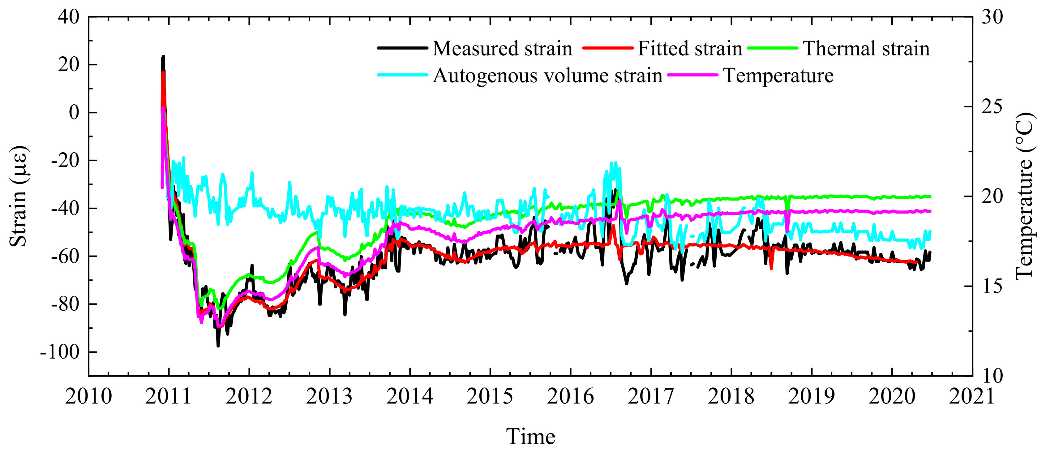
4.2. Change Law Analysis of Stress-Free Strain

The laws of the autogenous volume deformation of concrete in the three zones are similar. The measuring point NCP16-2 buried in zone B in monolith 16 was taken as an example to analyze the autogenous volume deformation. The measuring point is located in the middle of EL 411 m. According to Equation (6), the linear expansion coefficient and autogenous volume deformation were obtained by the least-squares method. The calculated linear expansion coefficient is 6.589 με/°C. As shown in Figure 6, the autogenous volume deformation shrinks first and then expands, and the measured value of autogenous volume deformation was finally stable at −60 × 10⁻⁶. The autogenous volume deformation is small.

4.3. Analysis of Stress Distribution and Variation Law

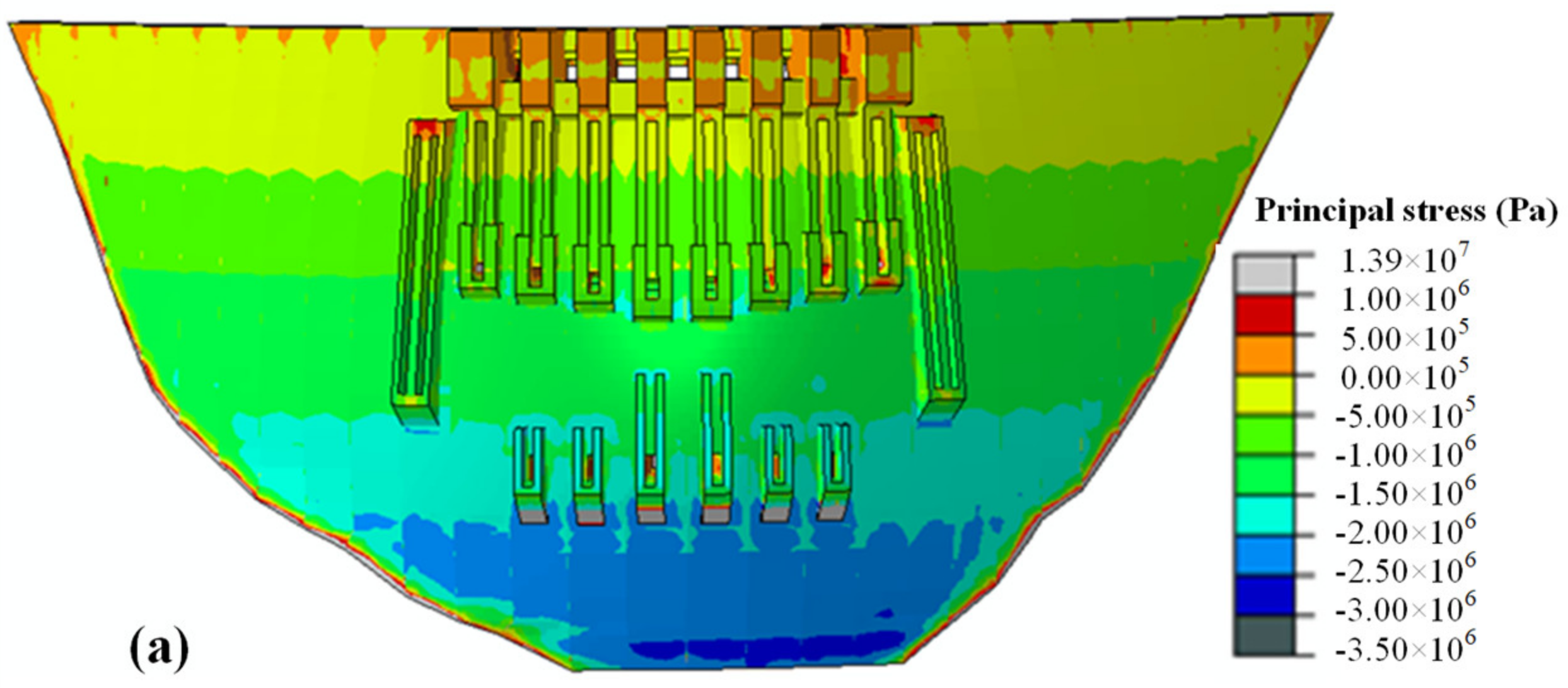
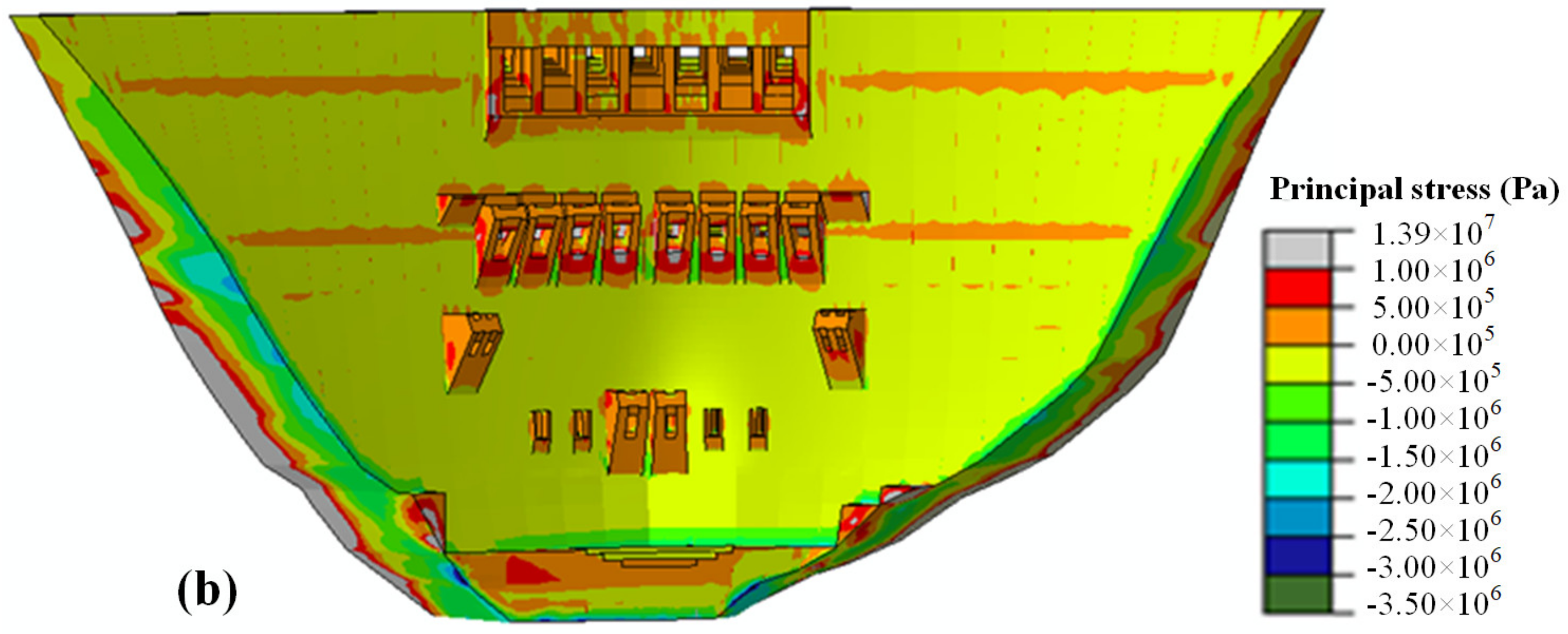
4.3.1. Design Stress Distribution

Both load and concrete properties affect the dam stress. Loads include thermal load, self-weight, hydrostatic pressure load, etc., and the concrete properties are related to creep, linear expansion coefficient, autogenous volume deformation, etc. [27,29,30].

According to the design data, the dam stress is controlled by the combined working conditions of normal RWL and temperature drop and dead RWL and temperature rise [24]. Under these two controlling conditions, most of the dam surface is under compression, and only the region around the foundation is in tension. Under the condition of normal RWL and temperature drop, the upstream surface is mostly in a relatively uniform compression state. The principal compressive stress on the upstream face gradually increases from the arch abutment to middle, and the compressive stress in most regions is −2–−6 MPa. The principal stresses of the left- and right-half arches of the upstream surface are symmetrical, and the high stress is located in the middle and lower regions of the dam. The principal tensile stress of the upstream face occurs within a small range, and only appears locally at the arch abutment of high elevations. The downstream surface is basically in a compressed state, the principal compressive stress distributes uniformly and increases from the middle to arch abutment, and the high stress is located at the dam toe with elevations of 332–440 m. The tensile stress is locally distributed only near the arch abutments for the downstream face.

Considering the high accuracy of deformation observation, the material properties of the dam and foundation rock mass were inverted using the deformation data, and the material parameters were obtained [24,31]. The idea is “deformation feedback and stress review”. Using the deformation data of the reservoir filling to EL 540 m (7 October 2013), the inversion analysis of the deformation parameters was carried out via the finite element method. The relevant deformation equipment arrangement and deformation observation data analysis were detailed in [6]. On this basis, the deformation and stress were analyzed via inverted parameters. The inverted parameters were used to calculate the stress distribution during the reservoir filling to EL 560 m (13 December 2013), EL 580 m (27 August 2014), and EL 600 m (28 September 2014).

The elastic modulus of dam concrete was still in slow growth. The inverted elastic modulus was 44 GPa. The inverted value was basically reasonable. The calculation results of monolith 16 (i.e., the crown cantilever monolith) are shown in Figure 7. Because the plumbline system at higher elevation was put into operation later, there is a certain error between the measured value and the predicted value.

Figure 8 shows the principal stress distribution on the upstream and downstream surfaces of the dam when the reservoir was impounded to EL 600 m. The maximum principal compressive stress on the downstream surface is 9.5 MPa, which occurs at the junction of the top of the left bank footing and the dam surface. As the RWL rises, the water load carried by the arch dam is gradually transferred to the two dam abutments.

According to the finite element analysis, the dam can be divided into five main stress control regions [32]: (a) The three-direction compression region, which is the main control region of the compressive stress on the upstream surface. This region ranges from 1/5 to 4/5 of the dam height of the crown cantilever monolith. (b) The tension–compression region under multiaxial stress near the upstream arch abutment, which is the tensile stress control region. This region is in two-direction tension and one-direction compression, or two-direction compression and one-direction tension. (c) The stress concentration region at the dam heel, which is also a key control region. (d) The main tensile stress region on the downstream face, where the main tensile stress along the cantilever direction is prone to occur due to the RWL change. This region is from 1/2 of the dam height to the dam crest. (e) The bi-directional compression region near the arch abutment of the downstream face, where the maximum compressive stress often occurs. This region is from 1/2 of the dam height to the foundation, and the width is about 1/4 the dam height.

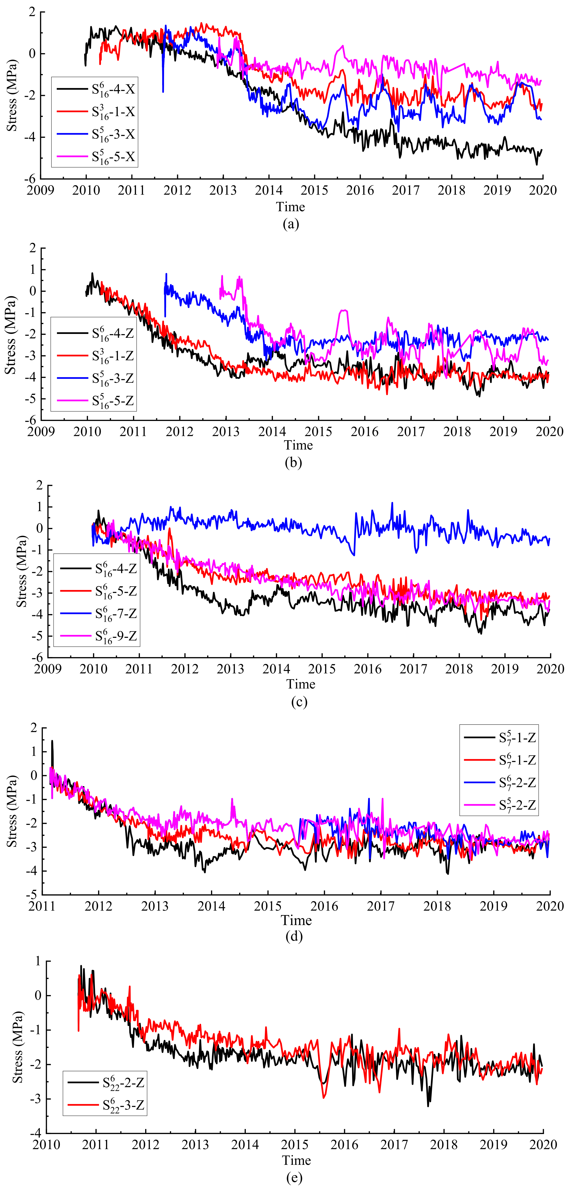
4.3.2. Spatiotemporal Distribution Characteristics Based on Measured Data

The reservoir experienced four filling–discharging cycles from 2013 to 2018. Reservoir filling leads to a complicated stress redistribution in both the arch and cantilever directions. The spatiotemporal distribution characteristics were analyzed based on the measured data.

The dam was in a compression state during the initial operation stage, and the global stress distribution was basically symmetrical. The arching effect was obvious. The z-direction compressive stress on the upstream side decreases with the rise of the RWL, and vice versa. Meanwhile, the z-direction compressive stress at the dam heel was the maximum when the RWL was EL 540 m. When the RWL rises, the x-direction compressive stress in the low-elevation of the dam increased significantly, and the arching restraint effect was strong.

The maximum value of the z-direction compressive stress was −9.09 MPa during the focused stage, which occurred at the upstream measuring point of monolith 18 at EL 334.4 m in May 2016, and the corresponding RWL was 547 m. The maximum x-direction compressive stress was −7.5 MPa, and this appeared at the downstream measuring point of monolith 16 at EL 442.2 m in October 2016, and the corresponding RWL was EL 600 m.

The analyzed time series of the stress ranges from the construction period to the end of 2018. The measured stress was obtained via the conversion method described in Section 2.1 and the fitted results in Section 4.1. The historical processes of the measured x- and the measured z-direction stress of the upstream side points of monolith 16, along with the x-direction stress at the dam heels of monoliths 7, 16, and 22, are shown in Figure 9. For further explanation, two typical measuring points were selected, namely, S⁶₁₆-4-Z at EL 334.4 m in the extended deep excavation region of the dam foundation and S⁵₁₆-3-X at EL 481.2 m in the middle of the upstream surface of monolith 16, to show the relationship between the RWL and stress in different directions at different locations. The corresponding historical process is shown in Figure 10.

Measured data show that the z-direction stress in the upstream restraint region was in a compressed state. During the construction stage, the z-direction compressive stress increased gradually with the increase in dam height. The z-direction stress in the upstream restraint region gradually decreased from the riverbed to the abutment and generally decreased with the rise of the RWL, but it was still in a state of compressive stress. The measured value was between −8.06 and −0.37 MPa. The x-direction stress in the upstream restraint region was in a compressed state and increased slightly with the rise of the RWL. The tensile stress in the x-direction mainly occurred during the construction stage and then gradually became compressive stress. With the rise of the RWL, the x-direction compressive stress continued to increase, and that of the low-elevation increased significantly. During the filling process, the z-direction stress at EL 442.20 m and 481.20 m increased significantly. It can be seen that the arch thrust increased significantly with the rise of the RWL, and the arching effect was obvious. After July 2015, the x-direction compressive stress still increased slowly but gradually stabilized.

The z-direction stress in the downstream restraint region was in a compressed state, gradually decreasing from the riverbed to the abutment and slightly increasing as the RWL rises. The x-direction stress in the downstream restraint region was all under compression, and it also increased slightly with the rise of the RWL.

The z-direction stress of the crown cantilever (monolith 16) generally shows a decreasing trend from lower to higher elevation. The distribution law of the x-direction stress in monolith 16 was not obvious. When the RWL reached EL 600 m, the z- and the x-direction stresses increased compared with the RWL of EL 540 m.

Based on the analyses of the above representative regions, it can be seen that the z- and the x-direction stresses were in a compression state. The x-direction compressive stress still showed a certain development trend but tended to be stable. The tensile stress and the compressive stress on both upstream and downstream sides were relatively small. On the whole, the stress distribution of the dam was normal, and the stress variation law conformed to the engineering experience. It is worth noting that the stress observation results of many super-high arch dams, such as Xiluodu, Jinping I, Xiaowan, and Ertan all show that the dam heel was in a compression state under the action of its own weight and reservoir water load.

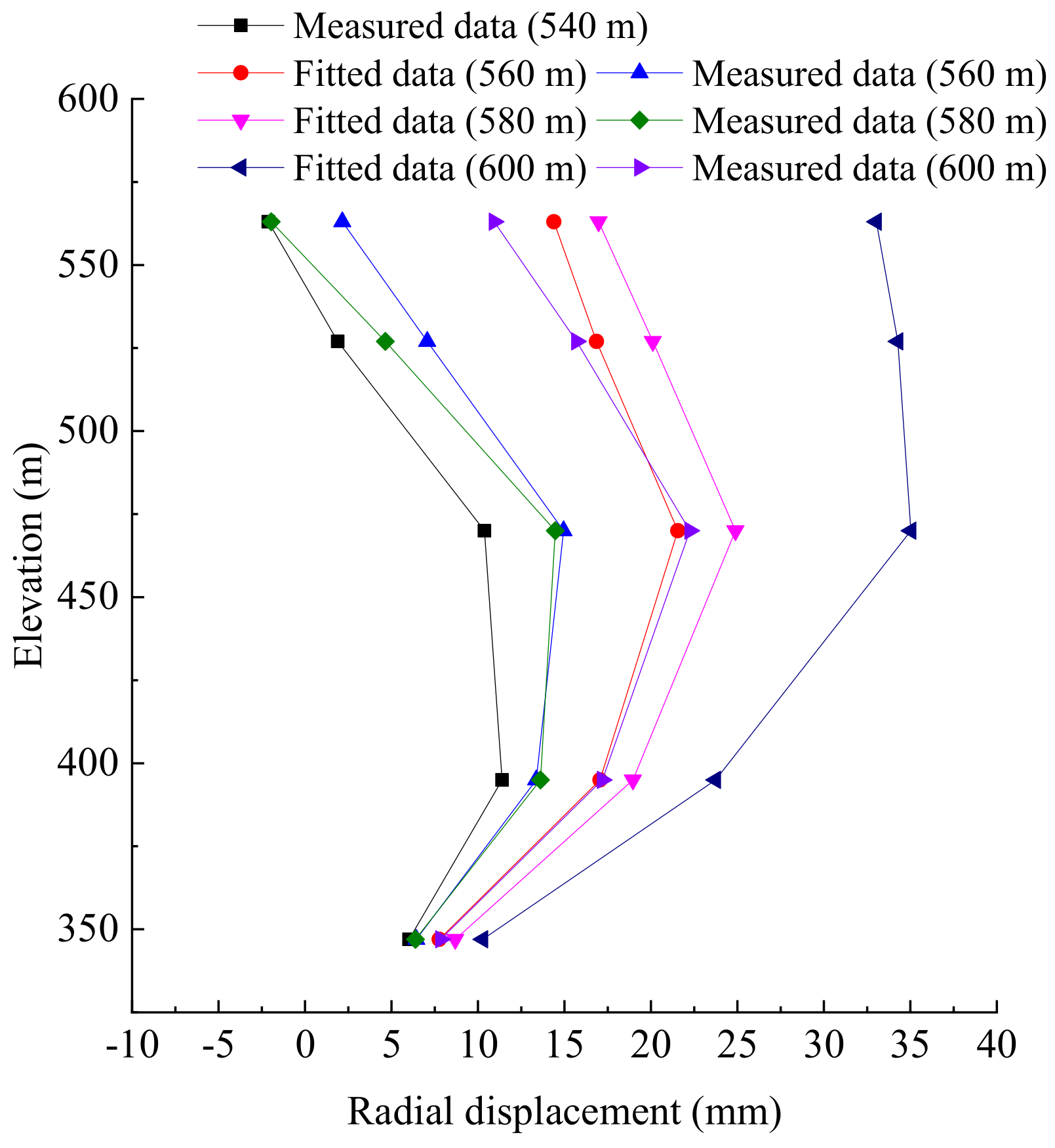
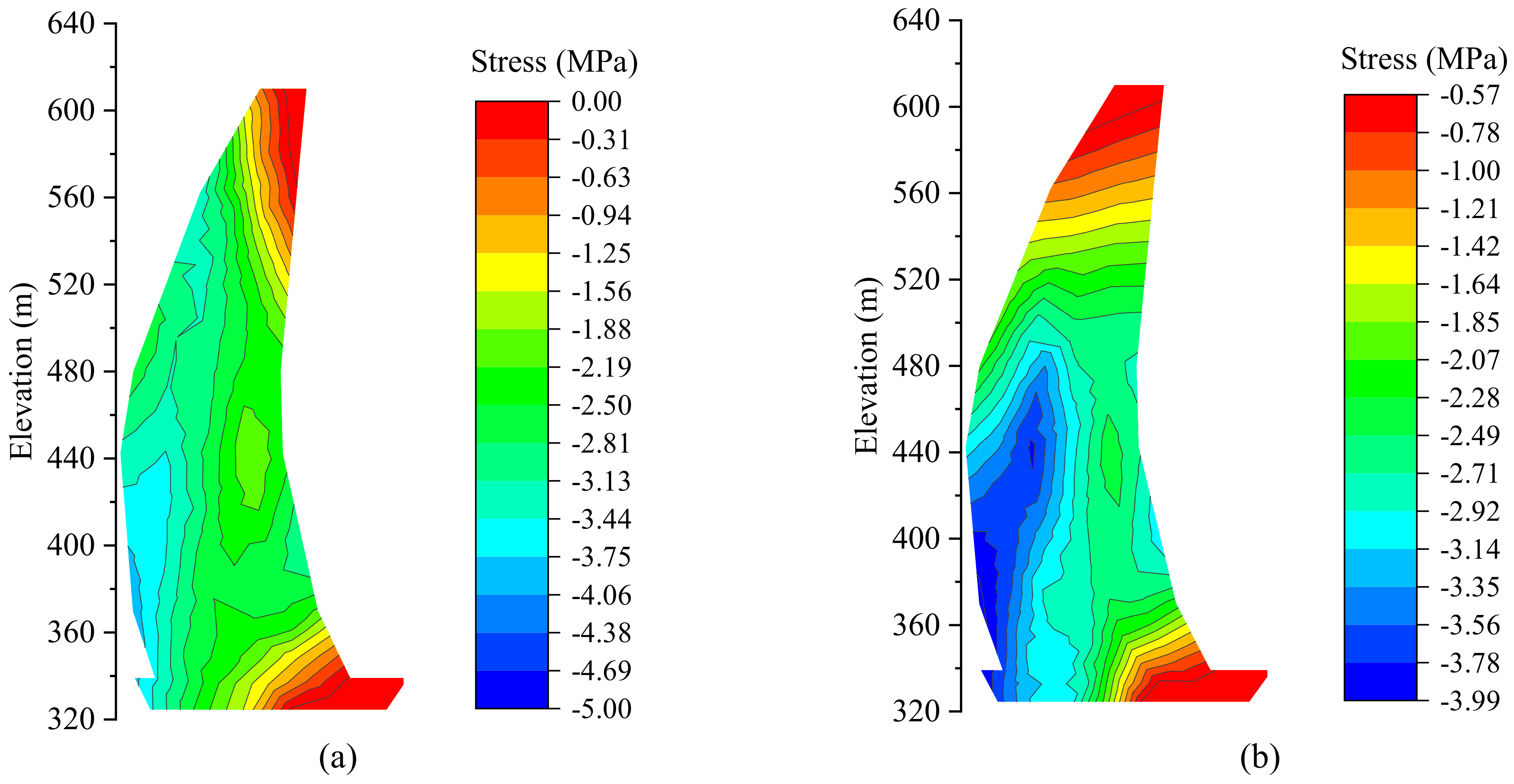
4.3.3. Stress Distribution and Variation Characteristics of Crown Cantilever Monolith

The stress at the dam heel is a key control index. Excessive tensile stress would cause the dam heel to crack, and in severe cases, would damage or even destroy the anti-seepage curtain, jeopardizing the dam safety. Selecting 5 October 2014 (the RWL was 599.27 m) and 15 June 2015 (the RWL was 545.34 m), the contour map of the z-direction stress of monolith 16 was drawn based on the measured stress, shown in Figure 11. When drawing the contour map, the measuring points were used as the control points, and the stresses of other regions were calculated by the radial basis function method. Since there was no measuring point above EL 562.2 m of monolith 16, the stress calculated via interpolation near the dam crest was less accurate.

The z-direction stress of monolith 16 generally decreased from low to high along the elevation. The z-direction compressive stress in the upstream side of the dam decreases as the RWL rises, and vice versa. Since the filling, when the RWL was near EL 540 m, the z-direction compressive stress at the dam heel generally reached the maximum value of the entire filling–discharging cycle. For the upstream measuring points of monolith 16, the maximum z-direction compressive stress was 4.89 MPa, which occurred on 25 June 2018 (the RWL was 554.98 m) at the measuring point S⁶₁₆-4-Z. The maximum variation, which was 2.50 MPa, occurred at the measuring point S⁵₁₆-3-Z in 2013. After that, the value stabilized at about 1 MPa.

During the filling process, the x-direction compressive stresses of monolith 16 had a certain increasing trend as a whole, and those of the central elevation measuring points were more significant. The maximum compressive stress on the upstream side was 5.32 MPa, which occurred on 12 November 2019 (the RWL was 594 m) at the measuring point S⁶₁₆-4-X. The largest variation occurred at the measuring point S⁵₁₆-3-X, and the largest annual variation, which was 3.56 MPa, occurred in 2013. After that, the annual variation was stable between 1.87 and 2.75 MPa.

At present, both the z- and x-direction stresses of monolith 16 are compressive stresses.

5. Construction of Stress Safety Monitoring Model

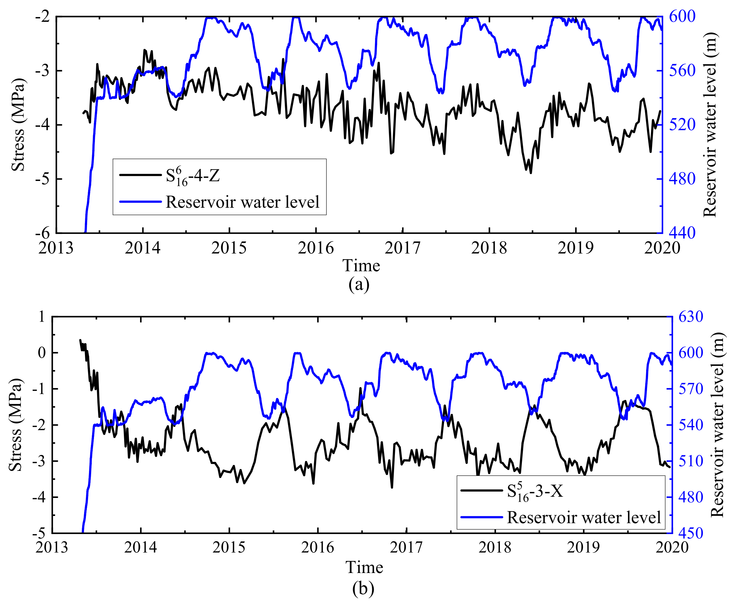
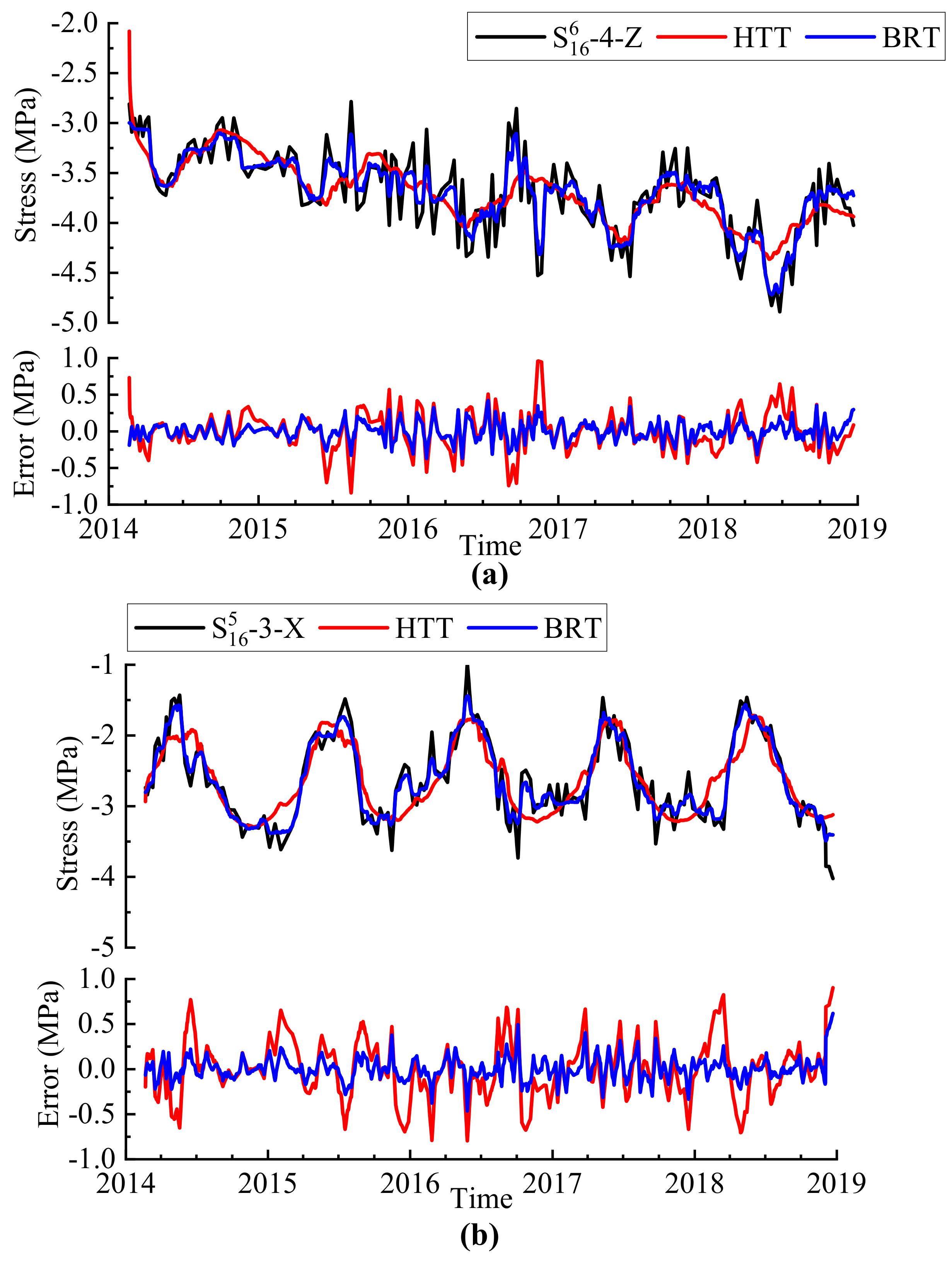
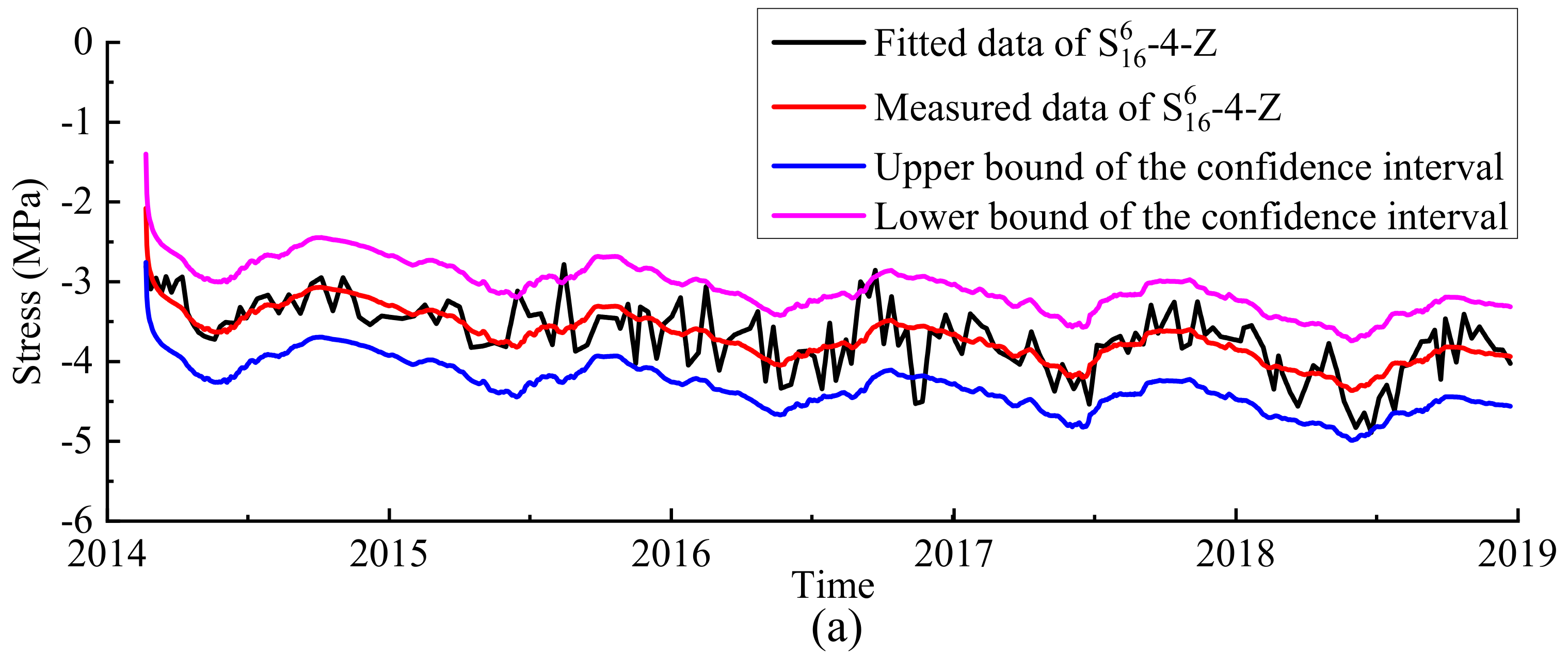
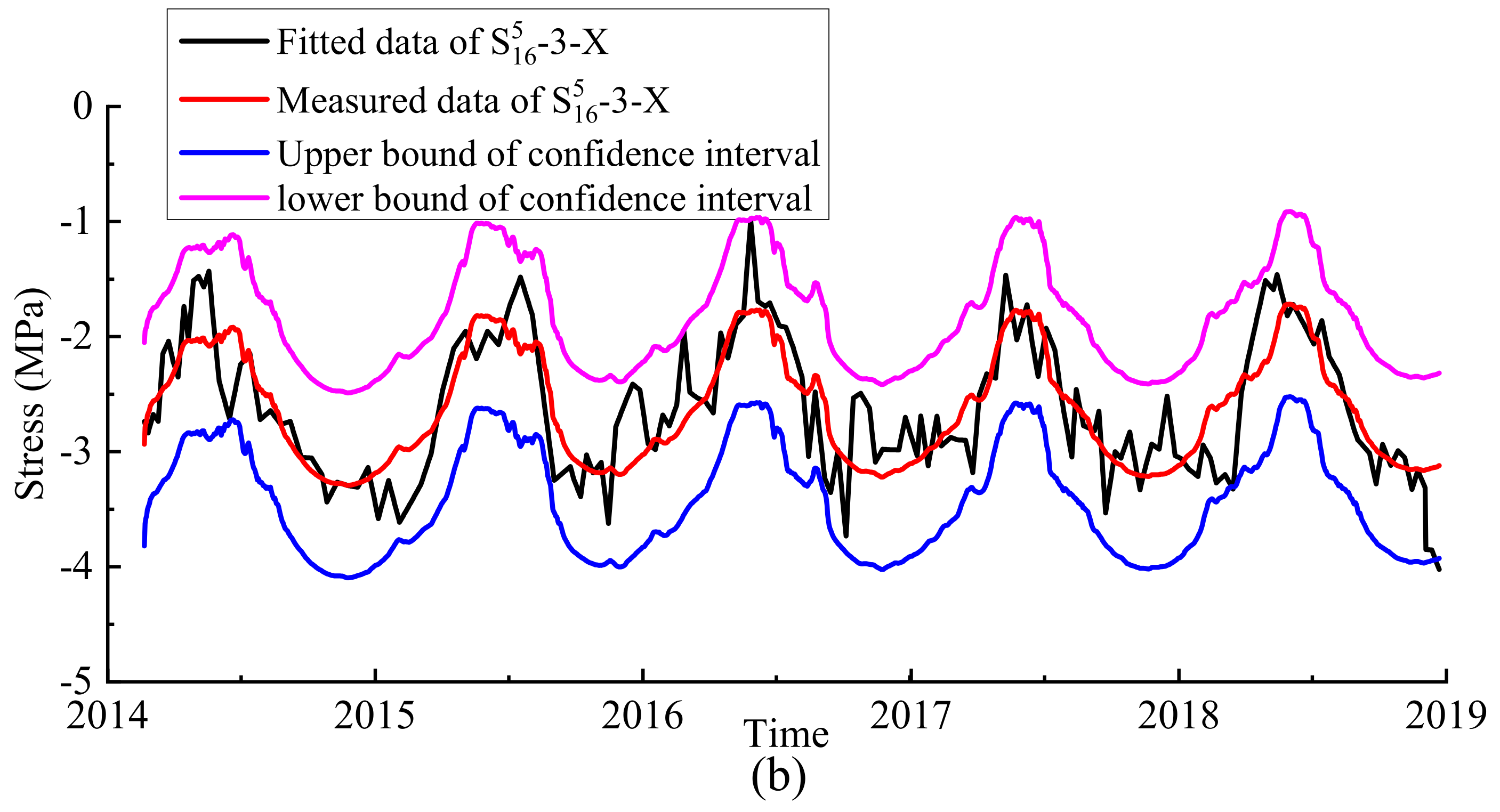
5.1. Quantitative Analysis and Prediction Based on HTT and BRT Models

The measuring points S⁶₁₆-4-Z and S⁵₁₆-3-X were selected. The time series used to build the HTT and the BRT models was from 6 March 2014, after the dam was completed, to the end of 2018. The influencing factors selected by the two models are the same. For temperature factors, in addition to the temperatures of this measuring point and the adjacent strain gauge groups, the nearby RWT was also selected. Specifically, not only was the temperature of the measuring point selected, the temperatures of the measuring points S⁶₁₆-5 and S³₁₆-1 and the nearby RWT were also selected for the measuring point S⁶₁₆-4-Z. In addition to the temperature of the measuring point, the temperatures of the measuring points S⁵₁₆-1 and S⁶₁₆-3 and the nearby RWT were also selected for the measuring point S⁵₁₆-3-X.

Considering that the dam was still in the initial operation stage, the last 5% samples of the time series were selected as the prediction test set. Figure 12 shows the fitting, prediction results, and residuals of the two types of built models for the two measuring points. In addition to the correlation coefficient, the fitting effect of the model was also analyzed via the mean absolute error (MAE). The fitting effect indicators are listed in

Table 4. Comparison of the fitting accuracies of the built models.

Point	HTT				BRT
	Training		Prediction		Training		Prediction
	R2	MAE (MPa)	R2	MAE (MPa)	R2	MAE (MPa)	R2	MAE (MPa)
S616-4-Z	0.643	0.521	0.617	0.463	0.90	0.223	0.86	0.262
S516-3-X	0.787	0.311	0.706	0.384	0.96	0.085	0.91	0.216

.

Based on the HTT model, the components of water pressure, temperature, and TDE were separated, and the relative influences of influencing factors on the stress are shown in Figure 13. It can be seen that the measuring point S⁶₁₆-4-Z in the extended deep excavation region of the foundation was significantly affected by temperature. This is related to the obvious temperature recovery in the low-elevation region since the first filling. The measuring point S⁵₁₆-3-X was significantly affected by the RWL, which is related to the increase in the arching effect of the middle elevation in the upstream side. Compared with the operation stage, the stress during the initial operation stage is significantly affected by the TDE.

The temperature rise increases the compressive stress at the dam heel by about 0.3 MPa. Correspondingly, the tensile stress at the dam toe increases, and the z-direction compressive stress at the dam toe decreases by about 0.13 MPa.

Further, the annual maximum compressive stress of each measuring point was analyzed. The annual maximum compressive stresses of the measuring points S⁶₁₆-4-Z and S⁵₁₆-3-X with the corresponding RWL are shown in Figure 14. According to the RWL process (Figure 5) and the reservoir scheduling, the RWL reaches EL 600 m in October every year, and the RWL drops to EL 540 m in June of the following year. The annual maximum compressive stress of the measuring point S⁶₁₆-4-Z generally occurs in late June, which is in the condition of low RWL and high temperature. The annual maximum compressive stress of the measuring point S⁵₁₆-3-X generally occurs in the condition of high RWL and low temperature.

The stress and distribution of a super-high arch dam during the initial operation is complex. The PDPs allow for the identification of the influence mechanisms of the predictor variables on the dam stress and can be used to judge whether the stress distribution conforms to the general law. The PDPs of the typical predictor variables for S⁶₁₆-4-Z and S⁵₁₆-3-X, including RWL, RWT, and TDE, are shown in Figure 15. In general, the relationships between stress and predictors are nonlinear and complex. In comparison, the stress mechanism of the z-direction is more complicated than that of the x-direction. Especially when the RWL is below EL 570 m, the z-direction stress does not increase monotonously. On the whole, the z-direction compressive stress caused by TDE increases. However, this effect is affected by many factors such as reservoir bottom deformation, valley deformation, water pressure, and environmental temperature, and is thus more complicated.

5.2. Stress Monitoring Index Based on Confidence Interval

Based on the constructed HTT model, the confidence interval estimation method was used to determine the monitoring indicators of stress. Considering that there are several factors affecting the stress during the initial operation stage, the significance level was taken as α = 1%. The interval range results of the measuring points S⁶₁₆-4-Z and S⁵₁₆-3-X are shown in Figure 16. It can be seen that the measured data fluctuate frequently due to complex environmental factors. The accuracy of the constructed HTT model is slightly lower than the operation period, which also directly affects the rationality of the confidence interval formulation. Specifically, the fitting accuracy of the HTT model of the measuring point S⁵₁₆-3-X is relatively high. The proposed monitoring indicator of this measuring point has a good guiding value for project management. Relatively speaking, the measuring point S⁶₁₆-4-X fluctuates frequently. The proposed monitoring index of this measuring point is only used as a reference for daily operation management.

5.3. Result Analyses and Discussions

The measured stress of the dam was obtained using the strain measured by the strain gauge group and stress-free gauge. Affected by various factors such as the absence of stress, the measurement accuracy of the strain gauge group, the elastic modulus of concrete, and the data processing method of autogenous volume deformation, there may be a certain deviation between the converted and the actual stress values. At the same time, the stress during the initial operation stage was affected by several factors. These factors include the rise of the interior temperature of the dam and the fluctuation of the RWT. The arching stress of the middle elevation upstream of the crown cantilever was significantly affected by the RWL, and the arching effect was obvious. In addition, the concrete temperature at this location did not show a significant recovery. The accuracy of the HTT model at this measuring point was high, and the monitoring indicators determined via the confidence interval estimation method have good guiding significance. Relatively speaking, there was a significant temperature rise in the extended deep excavation area of the dam foundation. The accuracy of the HTT model of the measuring point at this location is relatively low, and the proposed monitoring indicators are only of reference value.

6. Conclusions

The stress monitoring of a super-high arch dam during the initial operation stage is particularly important. Based on the observation data, the spatiotemporal distribution characteristics of the Xiluodu Dam during the initial operation stage were analyzed, and the monitoring indicators based on the confidence interval estimation method were determined. The main conclusions are as follows:

• The stress was in a relatively compression state. The stress along the cantilever direction within the upstream restraint area was in a compressive state, and the region of greater compressive stress was located at the middle elevation. The maximum of the principal compressive stress appeared at the middle elevation of the upstream face of the crown cantilever monolith. After the reservoir was impounded, the arching compressive stress showed an increasing trend, and the arching effect was obvious.
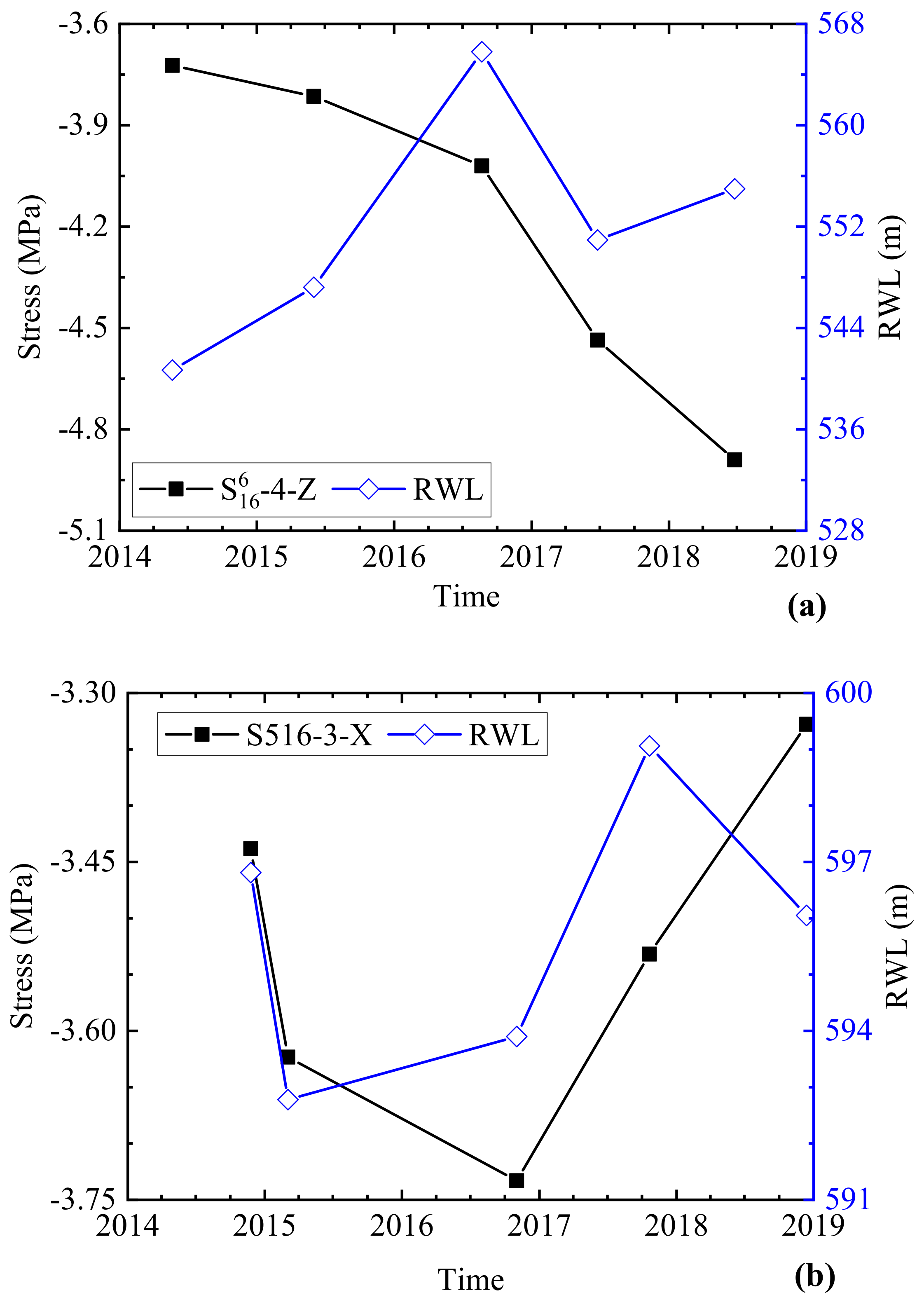
• The fitting accuracy of the HTT model for the measuring points where the temperature was relatively stable and the stress was significantly affected by the RWL was higher, and vice versa. The BRT-based model can significantly improve prediction accuracy. The principal stresses of the measuring points at different elevations and different locations are affected by the environmental factors in different mechanisms. The cantilever direction stress at the dam heel of the crown cantilever is significantly affected by the interior temperature recovery, and the arch direction stress at the middle elevation of the upstream side is significantly affected by the RWL.
• The stress of the super-high arch dam during the initial operation stage is affected by several factors, such as the rise of the internal temperature and the change of the RWT, and frequently fluctuates. Therefore, because the stress of the super-high arch dam during this stage is also affected by the valley deformation, the measuring points of the key locations with reliable measurement values should be selected for stress analysis, model construction, and monitoring index determination to guide the initial operation. In the future, the influence of valley deformation should be also considered when analyzing the stress of a super-high arch dam.
• The dam is prone to expose safety problems during the initial operation stage. Super-high arch dams need to withstand huge water loads, safety monitoring during this stage is more important, and attention should be paid to stress and deformation monitoring within 3 years after reaching the normal RWL. In addition to global climate change, extreme meteorological events exhibit a trend of high frequency and intensity. For super-high arch dams that are sensitive to the environment, stress monitoring deserves more attention.
• Although this paper has conducted a relatively systematic analysis from several perspectives, namely, data conversion, stress distribution, and prediction model construction of key measurement monitoring points, considering the development of data mining and artificial intelligence technology, future research should focus on proposing more convenient data processing methods, better result display formats, and better interpretation methods.

References

1. Wang, R.K. Key technologies in the design and construction of 300 m ultra-high arch dams. Engineering 2016, 2, 350–359. [Google Scholar] [CrossRef]
2. Wu, S.Y.; Cao, W.; Zheng, J. Analysis of working behavior of Jinping-I Arch Dam during initial impoundment. Water Sci. Eng. 2016, 9, 240–248. [Google Scholar] [CrossRef]
3. Jiang, H.; Zhang, C.-H.; Zhou, Y.-D.; Pan, J.-W.; Wang, J.-T.; Wu, M.-X.; Fan, Q.-X. Mechanism for large-scale canyon deformations due to filling of large reservoir of hydropower project. Sci. Rep. 2020, 10, 12155. [Google Scholar] [CrossRef] [PubMed]
4. Cheng, L.; Liu, Y.R.; Yang, Q.; Pan, Y.W.; Lv, Z. Mechanism and numerical simulation of reservoir slope deformation during impounding of high arch dams based on nonlinear FEM. Comput. Geotech. 2017, 81, 143–154. [Google Scholar] [CrossRef]
5. Prakash, G.; Sadhu, A.; Narasimhan, S.; Brehe, J.-M. Initial service life data towards structural health monitoring of a concrete arch dam. Struct. Control Health Monit. 2018, 25, e2036. [Google Scholar] [CrossRef]
6. Hu, J.; Ma, F. Statistical modelling for high arch dam deformation during the initial impoundment period. Struct. Control Health Monit. 2020, 27, e2638. [Google Scholar] [CrossRef]
7. Hu, J.; Ma, F. Comparison of hierarchical clustering based deformation prediction models for high arch dams during the initial operation period. J. Civil. Struct. Health Monit. 2021, 11, 897–914. [Google Scholar] [CrossRef]
8. Tao, Z.; Liu, Y.; Yang, Q.; Wang, S. Study on the nonlinear deformation and failure mechanism of a high arch dam and foundation based on geomechanical model test. Eng. Struct. 2020, 207, 110287. [Google Scholar] [CrossRef]
9. Liu, Y.; Zhang, G.; Zhu, B.; Shang, F. Actual working performance assessment of super-high arch dams. J. Perform. Constr. Facil. 2016, 30, 04015011. [Google Scholar] [CrossRef]
10. Lin, P.; Zhou, W.; Liu, H. Experimental study on cracking, reinforcement, and overall stability of the Xiaowan Super-High Arch Dam. Rock Mech. Rock Eng. 2015, 48, 819–841. [Google Scholar] [CrossRef]
11. Hellgren, R.; Malm, R.; Ansell, A. Performance of data-based models for early detection of damage in concrete dams. Struct. Infrastruct. Eng. 2021, 17, 275–289. [Google Scholar] [CrossRef]
12. Panicker, K.J.; Nagarajan, P.; Thampi, S.G. Critical review on stress-sensitivity and other behavioral aspects of arch dams. In Advances in Civil Engineering; Singh, R.M., Sudheer, K.P., Kurian, B., Eds.; Lecture Notes in Civil Engineering; Springer: Singapore, 2021; Volume 83. [Google Scholar] [CrossRef]
13. Liu, X.; Li, Z.; Sun, L.; Khailah, E.Y.; Wang, J.; Lu, W. A critical review of statistical model of dam monitoring data. J. Build. Eng. 2023, 80, 108106. [Google Scholar] [CrossRef]
14. Bukenya, P.; Moyo, P.; Beushausen, H.; Oosthuizen, C. Health monitoring of concrete dams: A literature review. J. Civil. Struct. Health Monit. 2014, 4, 235–244. [Google Scholar] [CrossRef]
15. Salazar, F.; Vicente, D.J.; Irazábal, J.; de-Pouplana, I.; Mauro, J.S. A review on thermo-mechanical modelling of arch dams during construction and operation: Effect of the reference temperature on the stress field. Arch. Comput. Methods Eng. 2020, 27, 1681–1707. [Google Scholar] [CrossRef]
16. Li, B.; Han, X.; Yao, M.D.; Tian, J.; Zheng, Q. Quantitative analysis method for the importance of stress influencing factors of a high arch dam during the operation period using SPA–OSC–PLS. Struct. Control Health Monit. 2022, 29, e3087. [Google Scholar] [CrossRef]
17. Zhang, G.X.; Liu, Y.; Zhou, Q.J. Study on real working performance and overload safety factor of high arch dam. Sci. China Ser. E 2008, 51, 48–59. [Google Scholar] [CrossRef]
18. Lin, P.; Shi, J.; Zhou, W.Y.; Wang, R.-K. 3D geomechanical model tests on asymmetric reinforcement and overall stability relating to the Jinping I super-high arch dam. Int. J. Rock Mech. Min. Sci. 2018, 102, 28–41. [Google Scholar] [CrossRef]
19. Luo, D.N.; Lin, P.; Li, Q.B.; Zheng, D.; Liu, H. Effect of the impounding process on the overall stability of a high arch dam: A case study of the Xiluodu dam, China. Arab. J. Geosci. 2015, 8, 9023–9041. [Google Scholar] [CrossRef]
20. Alembagheri, M. A study on structural safety of concrete arch dams during construction and operation phases. Geotech. Geol. Eng. 2019, 37, 571–591. [Google Scholar] [CrossRef]
21. Li, B.; Xu, J.; Xu, W.; Wang, H.; Yan, L.; Meng, Q.; Xie, W.-C. Mechanism of valley narrowing deformation during reservoir filling of a high arch dam. Eur. J. Environ. Civ. Eng. 2023, 27, 2411–2421. [Google Scholar] [CrossRef]
22. Sheibany, F.; Ghaemian, M. Effects of environmental action on thermal stress analysis of Karaj Concrete Arch Dam. J. Eng. Mech. 2006, 132, 532–544. [Google Scholar] [CrossRef]
23. Huang, Y.; Xiao, L.; Zhou, Y.; Ding, Y. How first-immersion age affects wet expansion of dam concrete: An experimental study. Int. J. Civ. Eng. 2021, 19, 441–451. [Google Scholar] [CrossRef]
24. Feng, Y.Q.; Shen, S.M.; Li, J. Report of the Design Unit of Xiluodu Hydropower Station—Safety Monitoring Section; Chengdu Engineering Corporation Limited: Chengdu, China, 2014. (In Chinese) [Google Scholar]
25. Hou, C.; Wei, Y.; Zhang, H.; Zhu, X.; Tan, D.; Zhou, Y.; Hu, Y. Stress Prediction Model of Super-High Arch Dams Based on EMD-PSO-GPR Model. Water 2023, 15, 4087. [Google Scholar] [CrossRef]
26. Kang, F.; Liu, X.; Li, J.J. Temperature effect modeling in structural health monitoring of concrete dams using kernel extreme learning machines. Struct. Health Monit. 2020, 19, 987–1002. [Google Scholar] [CrossRef]
27. Chouinard, L.E.; Bennett, D.W.; Feknous, N. Statistical analysis of monitoring data for concrete arch dams. J. Perform. Constr. Facil. 1995, 9, 286–301. [Google Scholar] [CrossRef]
28. Greenwell, B.M. Pdp: An R package for constructing partial dependence plots. R J. 2017, 9, 421–436. [Google Scholar] [CrossRef]
29. Jin, F.; Zhang, G.X.; Luo, X.; Zhang, C. Modelling autogenous expansion for magnesia concrete in arch dams. Front. Archit. Civ. Eng. China 2008, 2, 211–218. [Google Scholar] [CrossRef]
30. Hu, J.; Ma, F. Zoned deformation prediction model for super high arch dams using hierarchical clustering and panel data. Eng. Comput. 2020, 37, 2999–3021. [Google Scholar] [CrossRef]
31. Wang, S.; Xu, C.; Liu, Y.; Xu, B. Zonal intelligent inversion of viscoelastic parameters of high arch dams using an HEST statistical model. J. Civil. Struct. Health Monit. 2022, 12, 207–223. [Google Scholar] [CrossRef]
32. Li, Z. Study on Control Criteria of Stress and Integrity Safety of Super-High Arch Dams. Master’s Thesis, Tsinghua University, Beijing, China, 2010. [Google Scholar]
Figure 1. Arrangement of strain gauge groups: (a) three-direction strain gauge group; (b,c) types a and b of six-direction strain gauge groups; (d) five-direction strain gauge group.
Water 16 00746 g001
Figure 2. Calculation flow of measured stress for concrete dams.
Water 16 00746 g002
Figure 3. The Xiluodu Dam: (a) satellite photograph; (b) snapshot.
Water 16 00746 g003
Figure 4. Layout plan for engineering and stress monitoring: (a) engineering and stress monitoring; (b) dam concrete zoning and stress monitoring; (c) strain gauge groups in monolith 16.
Water 16 00746 g004aWater 16 00746 g004b
Figure 5. The change process of the RWL during the initial operation stage.
Water 16 00746 g005
Figure 6. Historical change of measured and fitted values of stress-free gauges.
Water 16 00746 g006
Figure 7. Comparison of measured and calculated radial deformations of monolith 16.
Water 16 00746 g007
Figure 8. Calculation results of principal stress distributions of the dam: (a) upstream surface; (b) downstream surface.
Water 16 00746 g008aWater 16 00746 g008b
Figure 9. Historical process of stress of the focused measuring points: (a,b) z- and z-direction stress of the measuring points of the upstream side of monolith 16; (ce) z-direction stress of the measuring points at the dam heels of monoliths 16, 7, and 22.
Water 16 00746 g009
Figure 10. Historical processes of the RWL and the stresses of typical measuring points: (a) z-direction stress of the point at the dam heel of monolith 16; (b) x-direction stress of the point on the middle of the upstream side (EL 481.2 m) of monolith 16.
Water 16 00746 g010
Figure 11. z-direction stress distribution of monolith 16: (a) 5 October 2014; (b) 15 June 2015.
Water 16 00746 g011
Figure 12. Fitted results and residuals of the two typical measuring points using the two models. Points using the two models: (a) S616-4-Z, and (b) S516-3-X.
Water 16 00746 g012
Figure 13. Relative weights of influencing factors on the stress of the two measuring points.
Water 16 00746 g013
Figure 14. Maximum compressive stress along the z- and x-directions and the corresponding RWL: (a) S616-4-Z; (b) S516-3-X.
Water 16 00746 g014
Figure 15. PDPs of (a) RWL, (b) TDE, and (c) RWL and TDE with S616-4-Z; (d) RWL, (e) RWT, and (f) RWL and RWT with S516-3-X.
Water 16 00746 g015
Figure 16. Upper and lower bounds of the measuring points: (a) S616-4-Z; (b) S516-3-X.
Water 16 00746 g016aWater 16 00746 g016b