1. Introduction
Climate change has produced an upsurge in high-intensity, short-duration rainfall events, increasing the threat of flash flooding through steeply sloped watersheds. These floods pose a hazard to natural watersheds and urban areas. Higher rainfall intensities increase the overland flow and may cause substantial damage to an area. Smaller (area = 5–50 km
2) steep-sloped watersheds or the upper regions of larger watersheds present a more significant risk due to the lack of hydrological data and a scarcity of management resources for preventative action [
1,
2]. When measured data are unavailable, numerical models can help predict flash floods. Several hydrological and hydrodynamic models were recently applied to predict overland flow [
3,
4,
5,
6,
7,
8]. Many of these models do not represent the complex flow processes of flash floods and have reduced complexity, increased parameter sensitivity, and reduced prediction accuracy [
9].
Natural, steep-sloped watersheds contain stream beds with woodland and meadow areas. Rainfall–runoff processes for these types of watersheds include rainfall, rainfall losses, and the remaining excess rainfall that turns into overland flow [
10,
11]. The excess rainfall comes from subtracting losses from the rainfall in the watershed. These losses are the interception (storage capacity of the canopy), surface storage, and infiltration into the unsaturated soil layer. In natural watersheds, rainfall intensity, land cover, and the unsaturated upper soil are the most important parameters to define the losses from a rainfall event [
1,
12,
13]. Surface storage in natural watersheds includes leaf litter interception and storage as well. During short, intense rainfalls, canopy interception, leaf litter, and near-surface infiltration may also reduce the short-term runoff and affect the overland flow ratio [
14,
15]. Accurately determining the runoff hydrograph at the outlet of these watersheds requires a better understanding of the physical processes of the losses from interception and leaf litter storage.
Forested watersheds have leaf litter layers with parameters that change over time (layer width, humidity, and storage capacity). The mechanism of leaf litter interception and how it stores and releases water is poorly understood [
16]. Most studies on leaf litter storage are empirical lab experiments based on a given watershed’s specific fauna [
17,
18,
19,
20,
21]. Further studies have combined lab experiments with different numerical approaches [
22,
23,
24]. Although studies have experimented with different leaf litter types worldwide, local vegetation can be compared to these measurements. The water retention in leaf litter depends on its current composition and thickness [
25]. The decomposition process will reduce a leaf litter’s storage capacity [
26]. The impact of leaf litter on runoff remains difficult to quantify; therefore, back calculations based on measured runoff are needed. This paper focuses mainly on leaf litter’s storage capacity as a function of initial conditions (dry or saturated) and rainfall intensity.
Various model structures, such as physics-based, index-based, and conceptual models, are available to describe rainfall–runoff processes in ungauged watersheds [
1]. Physics-based models can effectively assess and predict overland flow [
27]. Two-dimensional models applying shallow water equations may accurately predict runoff and flood occurrence timing and duration [
28]. They are computationally and data-intensive, and there is a need to evaluate the input parameters and rainfall–runoff processes to improve modeling success and avoid unnecessary uncertainty.
A proper model requires several components: (1) a precise topographic description because the slope geometry dictates the flow velocity; (2) detailed land use that defines the dominant vegetation, as well as seasonal land surface changes (e.g., cultivation, plowing, and harvesting); and (3) the temporal condition of land cover that may impede surface runoff, such as leaf litter or shallow channeling, or sediment deposition from previous runoff events. These components affect the quantity and rate of runoff on steep slopes [
29]. In addition to the fluid movement, the model must calculate the natural losses [
30,
31]. Including quick infiltration in the unsaturated upper soil layer can improve the shallow surface flow [
6,
32,
33,
34]. For calculating losses, different infiltration models have been included (Green and Ampt, CN) [
35]. Flash floods are not affected by slower processes such as transpiration or long-term infiltration.
Costabile et al., 2020 [
28], studied rainfall-induced floods in watersheds using the Hydrologic Engineering Centre River Analysis System (HEC-RAS). The current HEC-RAS version provides a valuable tool for complex modeling. The fully 2D computational model includes full hydrodynamical equations with an additional eddy-viscosity model. This model requires many input parameters to reproduce flow paths, times to concentration, and behavior of overland flow [
35,
36,
37,
38].
Findings from prior research were synthesized into a comprehensive model. While numerous studies propose applicable methodologies, they focus on watersheds that are larger than those examined. For larger watersheds, existing methods for evaluating overland flow are likely appropriate [
4,
5,
6,
7,
8,
9]. However, customizing the infiltration and surface storage volume is necessary for smaller, steeply inclined woodland watersheds. While hydrodynamic calculations for larger watersheds can be simplified [
4], the complexities of numerical methods and eddy viscosity play critical roles in ensuring accuracy for smaller, steep catchments [
6,
12,
32]. As previously discussed, the storage capacities of leaf litters show variability across different studies and experiments. These findings are instrumental in devising an approximation that can be seamlessly incorporated into a hydrodynamic model.
In this study on a gauged watershed, a complex depth-integrated model was evaluated using two rainfall–runoff events. In addition to the complex overland flow simulation, the model includes an infiltration add-in. Applying two modeling methodologies to incorporate interception and leaf litter storage, this study aimed to determine a better model for describing leaf litter losses during flash floods. The following section summarizes the forest rainfall–runoff processes and briefly introduces the study region.
Section 4 describes the rainfall–runoff methodology applied during modeling;
Section 5 presents prediction results and challenges.
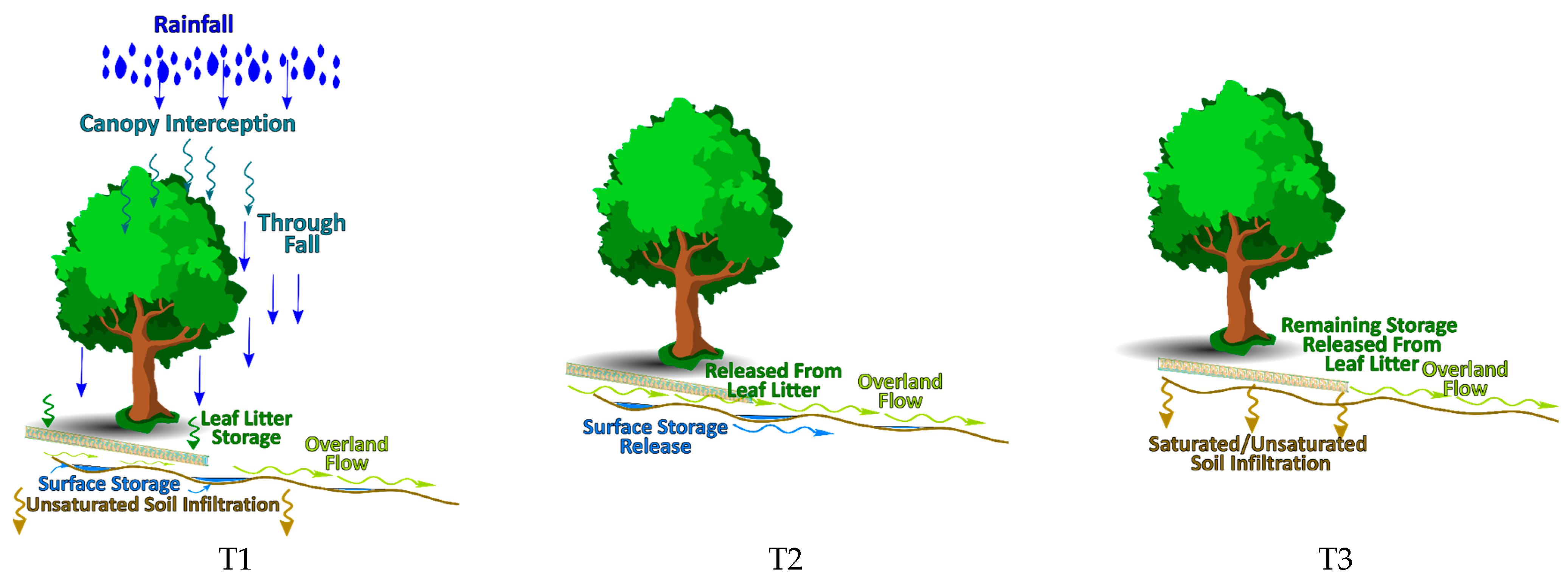
2. Forest Rainfall–Runoff Processes
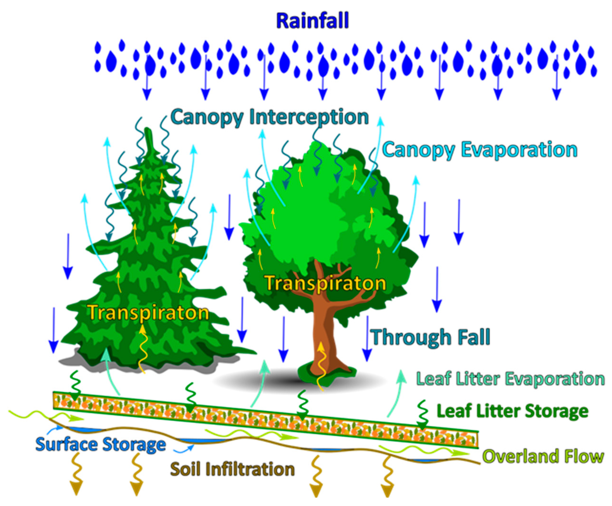
A natural, mainly forested watershed will store much water during and after rainfall. The canopy will intercept some rain while the rest continues as throughfall. The leaf litter then detains and stores some throughfall, while another portion passes through the leaves and reaches the ground’s surface. Finally, the remaining water may infiltrate the soil, collect in surface depressions (storage), or continue downhill as overland flow.
The quantity of rain involved in each process will depend on the rainfall intensity, the size and type (deciduous or coniferous) of the trees, the thickness and condition of the leaf litter, the irregularities in the ground surface, and the antecedent moisture in the soil. As the storage capacities in the canopy, leaf litter, and soil reach their limits, rainfall will convert directly into overland flow, initiating flooding conditions. Evaporation and transpiration processes are slow relative to short, violent bursts of rain, so they do not significantly reduce the quantity of overland flow during such events.
Figure 1 presents the conceptual model for forest rainfall hydrology.
This study focused on short-term, high-intensity rainfall events. Since watersheds are forested and have significant slopes, the main processes occur over a short period, in which soil infiltration has only a limited impact. Rainfall intensity and duration, canopy which soil infiltration has only a limited impact. Rainfall intensity and duration, canopy and leaf litter interception, surface storage, and slope steepness have the most significant effects on the occurrence and intensity of flash flooding. In small watersheds, short-duration, high-intensity rainfalls can cause floods.
A leaf litter layer forms in watersheds covered with forested areas. It has storage and infiltration capacities and becomes saturated during rainfall as it stores water. This water may then infiltrate the soil, remain on the surface, evaporate, or slowly release into overland flow. The processes occurring in leaf litters usually require a more extended period than a rainfall event. A leaf litter’s capacity changes seasonally and depends on its thickness and area distribution. In these cases, infiltration dominates the water’s movement.
In steep-sloped watersheds, the runoff volume and peak flow increase while the time to peak decreases. These types of watersheds are more susceptible to flash floods. The interception, depression storage, and soil infiltration capacity also decrease. In this paper, the authors considered watersheds with a 5–10% slope or higher and observed that, with an increasing slope, the infiltration decreased [
29].
Typical Sequence of Rainfall–Runoff Events
The rainfall–runoff process in a natural watershed can be visualized in three steps, as shown in
Figure 2. During a high-intensity rainfall (T1), rainfall breaks through the canopy and fills the leaf litter layer. Without a leaf litter layer (meadows, agricultural land), rainfall infiltrates the soil layer. If no leaf litter covers the ground, soil infiltration and surface ponding may begin. The depressions fill up on an uneven surface, and the water surface in these depressions starts to behave as a temporary impervious surface. At the same time, overland flow initiates, driven by the rainfall not captured by the other processes. A significant quantity of rainfall may directly convert to overland flow if the rainfall intensity is high.
At time T2, when the rainfall stops, the leaf litter layer slowly releases the stored water on the surface, producing overland flow. The water in the depressions filled during the rainfall starts infiltrating the soil layer.
Days after the rainfall (T3), the stored water in the leaf litter layer continues to release on the surface, and infiltration continues into the unsaturated soil layer. The water in the depressions also continues to infiltrate into the soil layer.
3. Study Area
3.1. Watershed Description
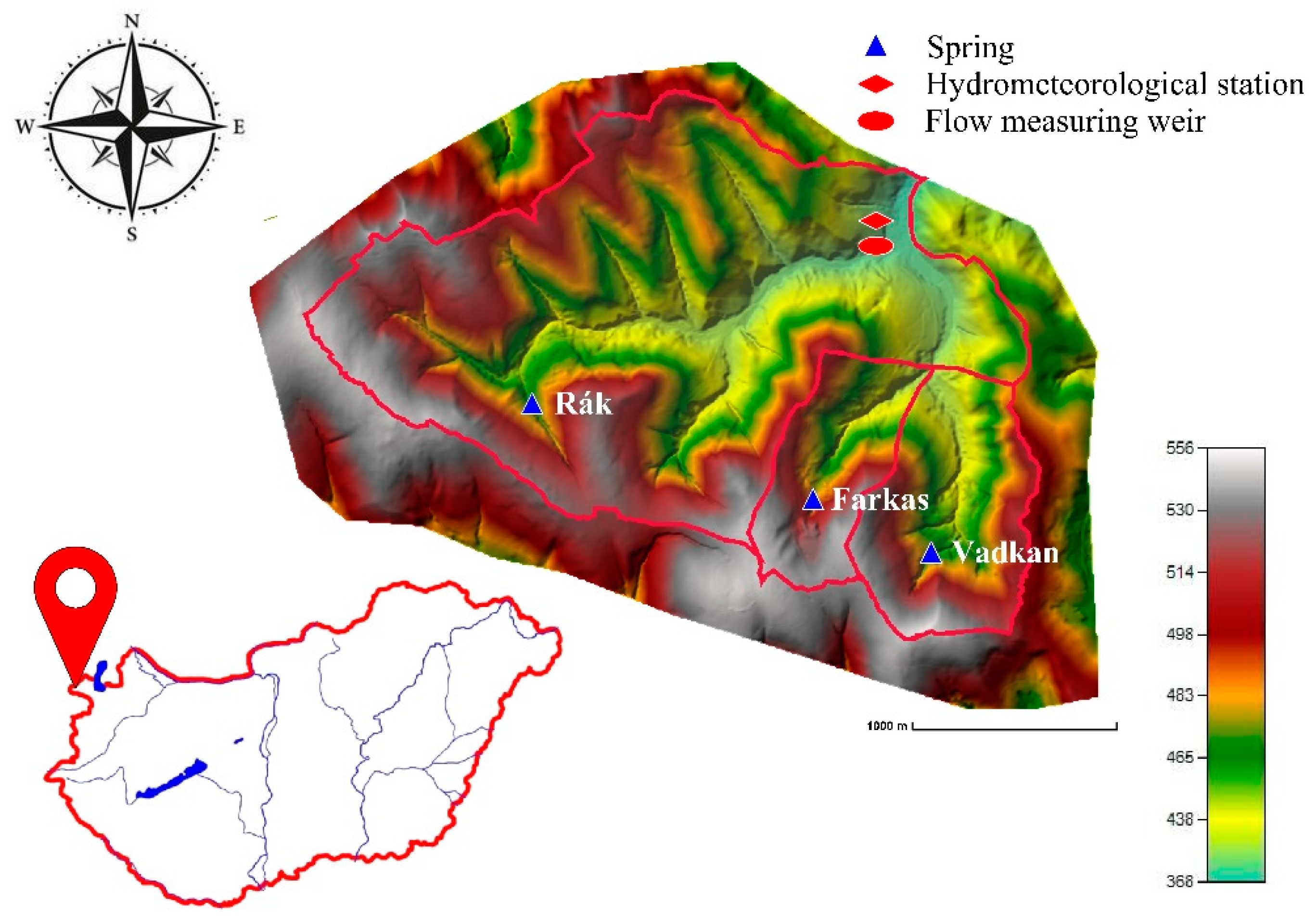
The Hidegvíz Valley extends over ~6 km
2 in the northwestern corner of Hungary. It is a small experimental watershed with dedicated hydrometeorological, overland flow, and infiltration measurement stations. The watershed consists of three subbasins formed by the confluence of three streams (
Figure 3).
From west to east, the Rák creek is the primary water body; the tributaries are the Farkas and the Vadkan are streams. The main channel length is ~3000 m, and the average bed slope is 4%. The Vadkan and Farkas Streams’ lengths are ~1400 and ~990 m, with an average 4–6% slope. More than 2/3 of the area of the three subwatershed belongs to the Rák Creek, 4.4 km
2; the Vadkan Stream comprises 0.93 km
2 and the Farkas Stream comprises 0.6 km
2. The entire watershed area is 6 km
2 [
39].
The Hidegvíz Valley lies within the Sopron Mountains. It has an average annual precipitation of 700–900 mm, with peak rainfall in July. The annual temperature averages 8–8.5 °C. The climate exhibits a strong subatlantic effect [
40]. The Köppen system classifies this region as Cfb (warm temperate, without dry season, and warm summer).
Although the watersheds are small, the streams are perennial, fed by springs. While researchers have not measured the springs’ flow rates, they have observed similar flows from all three.
The geology of the catchment is crystalline bedrock and Tertiary (Miocene) fluvial sediment deposited in five general layers. Podzolic brown forest soils, non-podzolic highly acidic soils, and lessivated brown soils (soil structure broken down by clay minerals leaching into the layer) have evolved in this area. These soil types are typical for cool, humid forest environments.
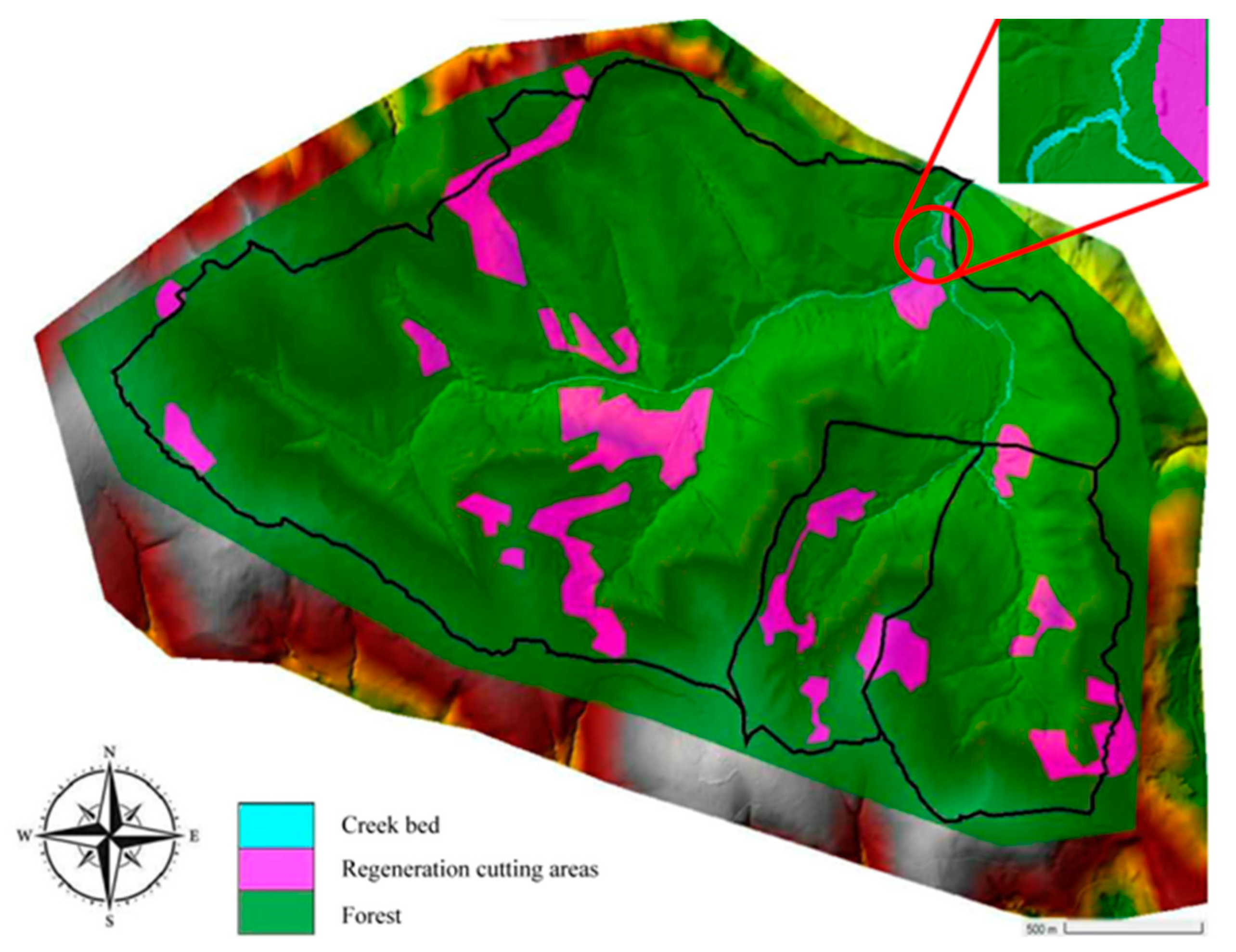
The natural forested areas in the watershed appear in
Figure 4. The primary woodland type was beech, with smaller oak (dashed line) and negligible pine areas (red) [
41]. In the 19th century, due to intensive afforestation, 50% of the woodland areas became needle-leaf wood areas [
42].
The meadow areas are generally open, containing smaller vegetation. The stream beds are natural; the only artificial structures are the culverts at the crossings of the forestry routes. Because of the erosion, the beds are winding, and the bed material is mainly rocky.
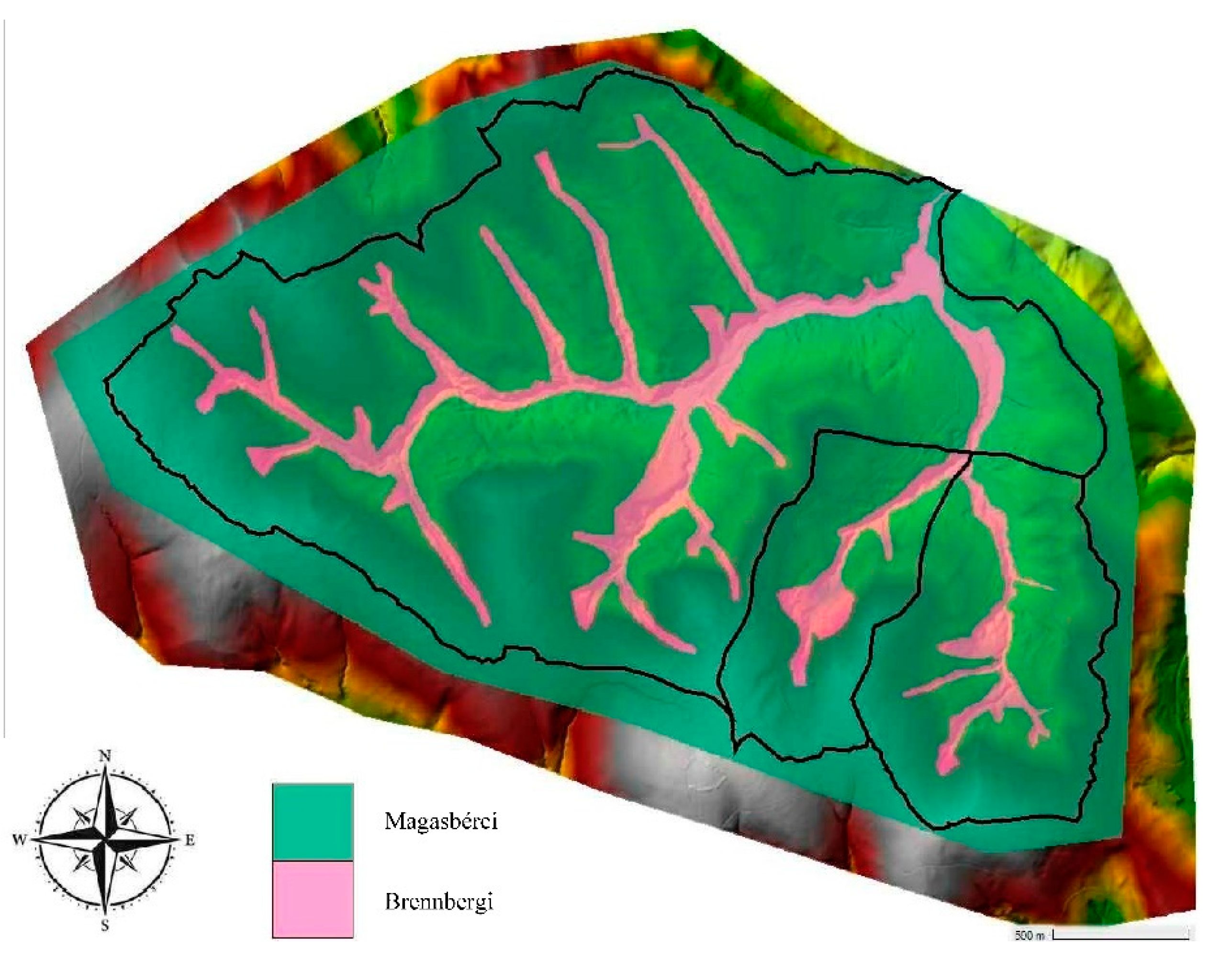
The watershed has two major soil types [
43]. “Magasbérci” formation soils cover the stream beds, while “Brennbergi” formation soils cover the rest of the watershed.
Figure 5 shows the distribution of the main soil types.
The “Magasbérci” (magenta) layer is primarily an alluvial loamy sand layer with fluvial gravel pockets. This soil covers only areas near stream beds [
44].
The “Brennbergi” (green) layer represents the higher parts of the watershed over the “Magasbérci” layer. The formation contains mostly blocks, with an average size of over 1 m; the blocks are sharp and cracked. Alluvial soil types have washed into the cracks, mainly loam, sand, and gravel debris. The soil layer’s proper composition is heavily unclassified [
44].
The root zone is 2–3 m deep. Since porosity is greater in woodland areas than in meadows, they have a higher water storage capacity [
44].
3.2. Measurements
Researchers have conducted meteorological, hydrological, and forest-related measurements and experiments on the watershed since 1983, with reliable data for modeling since 2010. Located near the Rák–Farkas Creek junction, the hydrometeorological station measures precipitation, temperatures, and wind speed. A broad-crested weir with a trapezoidal section measures the discharge flow nearby in the bed of Rák Creek, which is the combined flow from the Rák, Farkas, and Vadkan streams. Water levels in the stream are measured using pressure transducers with an absolute precision of ±2 mm, a sensitivity of ±0.1 mm, and a maximum depth of 1.5 m. Level readings occur at 1-minute intervals. The pressure transducers are manufactured by Dataqua Ltd. [
45]. The in situ and laboratory experiments for leaf litter interception also occurred at the station [
41].
4. Case Studies
Rainfall data at the Hidegvíz station was collected daily and at 10-minute intervals. The events between 2010and 2013 were evaluated based on the following criteria:
The cumulative one-day 10 min and daily measurements should match.
The intensity should be high enough to cause overland flow.
Measurement errors must be avoided; the full data set for rainfall and runoff and the time measurement of the events had to be correct.
Two events in July, Event 1 in 2010 and Event 2 in 2012, were selected for model prediction. Their rainfall intensities, durations, and volumes appear in
Table 1. Runoff volumes and rainfall/runoff volume ratios also appear in the table.
4.1. Event 1
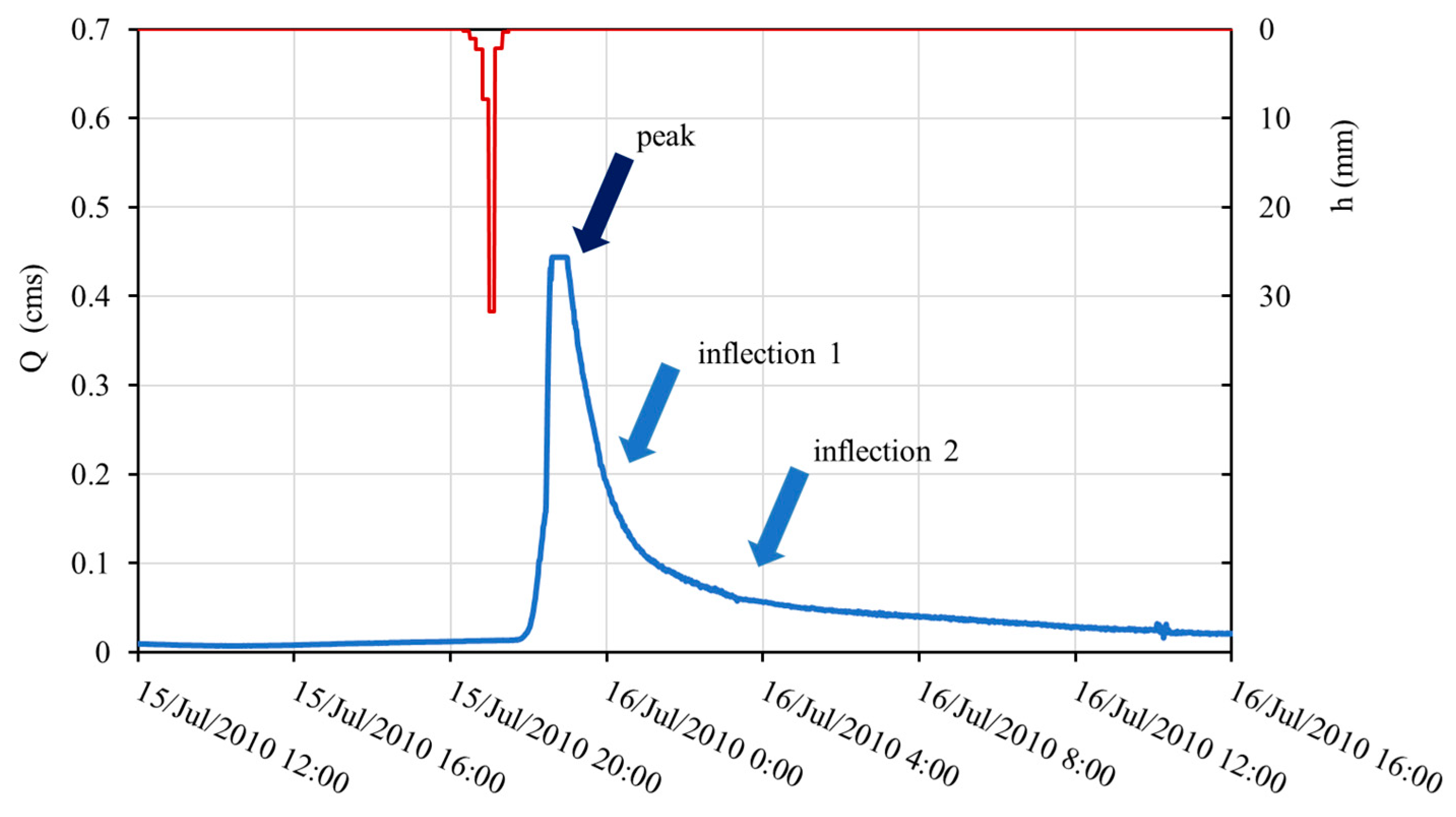
The rainfall started on 15 July 2010 at 20:20 and ended on 15 July 2010 at 21:30 (
Figure 6). The cumulative rainfall was 45.7 mm, totaling 70 min. Overland flow at the measuring station started at 21:47, and peak flow was reached between 22:38 and 22:59. During this time, the measurement weir did not record any flow. For this duration, we assigned a constant value of 0.44 m
3/s. The recession limb has two distinct inflection points. The first inflection point occurred on 15 July at 23:49; after this time, rapid overland flow drainage turned more gradual as interflow reached the outflow of the creek. There is a less-distinct change in the slope on 16 July at 3:39, when interflow starts to play a more dominant role. On 16 July at 16:00, the hydrograph reaches its minimum; the flow is close to the previous baseflow value.
Estimated time of concentration: 170 min (measured from the center of rainfall to the inflection point on the recession limb).
4.2. Event 2
The rainfall started on 7 June 2012 at 15:20 and ended on 7 June 2012 at 17:00 (
Figure 7). The cumulative rainfall was 53.4 mm, lasting 1 hour and 40 min. Overland flow at the measuring station started at 16:40, and peak flow was reached between 17:53 and 18:08. Between the two peaks, flow decreased for 8 min and increased again to reach the same peak 7 min later. The inflection point in the recession limb of the hydrograph is 19:09. The flow suddenly jumps lower at 22:00, then rises back up on 7 July at 1:53 a.m. The jump indicates a possible disturbance in flow measurement around the measuring weir. On the following day (7 July 2012) at 8:00, the hydrograph levelled off to the baseflow level. The estimated time of concentration is 210 min (center of rainfall, inflection point).
Even though both events occurred in July, there are distinct differences between the two hyetographs and hydrographs. For Event 2, precipitation had a longer duration but lower intensity. For Event 1, the maximum rainfall intensity was twice that of Event 2.
The runoff hydrograph shapes have similarities and differences; the rising limb increases sharply for both hydrographs, but the peaks and recession limbs differ. Since measurement error during Event 1 forced an assumed peak at 0.44 m3/s, comparing peak flows becomes problematic. The recession limb descends more gradually for Event 2 than for Event 1. There can be several reasons for the difference between the two events, such as (1) antecedent conditions in the catchment, (2) dissimilar rainfall intensities, and (3) different rainfall durations.
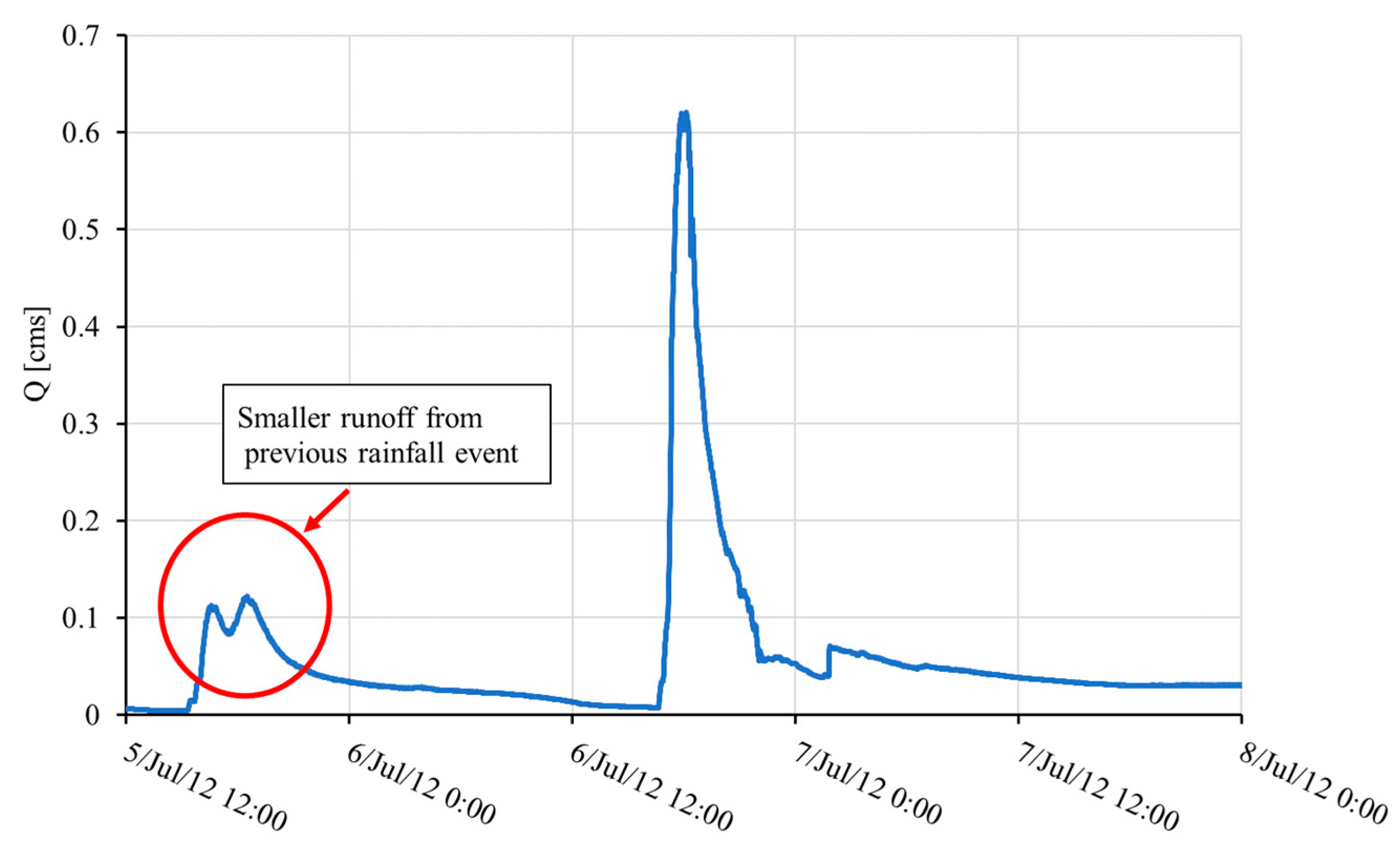
Several meteorological conditions influence antecedent conditions, but rainfall is the most significant. Two days before Event 2, two smaller rainfall events occurred, while no rainfall event occurred twenty days before Event 1. Therefore, the watershed was drier before Event 1 than Event 2. The rainfall before Event 2 produced measurable runoff, as shown in
Figure 8.
A smaller runoff event started on 5 July 2012 at 15:50. The decreasing flow becomes baseflow around 6 July 2012 at 12:00. According to Kiss [
41], the leaf litter releases water after rainfall. After the first 24 hours, there is a continuous outflow from the leaf litter. The flow decreases every day, but it lasts for several days. As a result, one can assume that for Event 2, the leaf litter storage was not empty, and the soil was not dry.
5. Materials and Methods
5.1. Canopy Interception and Leaf Litter Storage
For canopy interception, the following equation was used [
39]:
where
Ic [mm] = interception,
S [mm] = storage capacity of the canopy, and
h [mm] = rainfall height. The formula was designed for daily rainfalls and required adjustment.
Experimental data show that canopy interception decreases linearly with time during rainfall [
22]. The linear decline is important for long-duration rainfalls; however, this study investigated short rainfall events, and the canopy interception capacity remained constant.
Various experiments determined leaf litter interception parameters using needle-leaf and broadleaf litter materials. Both types exist in the Hidegvíz Valley watershed. According to experiments presented in [
41], leaf litter behaves like a sponge, drawing up and releasing water during and after rainfall. Csáfordi et al. [
39] estimated litter interception to be a linear process with time.
Kiss [
41] determined a formula for leaf litter storage from experiments in the Hidegvíz watershed. The following equation was derived based on leaf litter in the Hidegvíz Valley:
where
Es [mm] = leaf litter interception,
Sa [mm] = maximum storage capacity of the leaf cover,
Th [mm] = rainfall height, and
n = is the dimensionless factor. Equation (6) does not consider the increased leaf litter storage with time. The loss of the stored water from leaf litter is around 0.5 mm in a day. Similarly to Equation (1), this formula considers daily rainfalls [
41].
Zhao et al.’s [
22] experiments have shown a connection between rainfall duration and litter storage capacity in different sloped areas. They later investigated forests with two wood types: Magnolia grandiflora and Pinus massonlana [
22]. They found that leaf litter storage depended on the watershed slope. The experiment used different litter masses for slopes 5° and 20°. At the Hidegvíz Valley, the average slope of the watershed area is around 10°.
Li et al. [
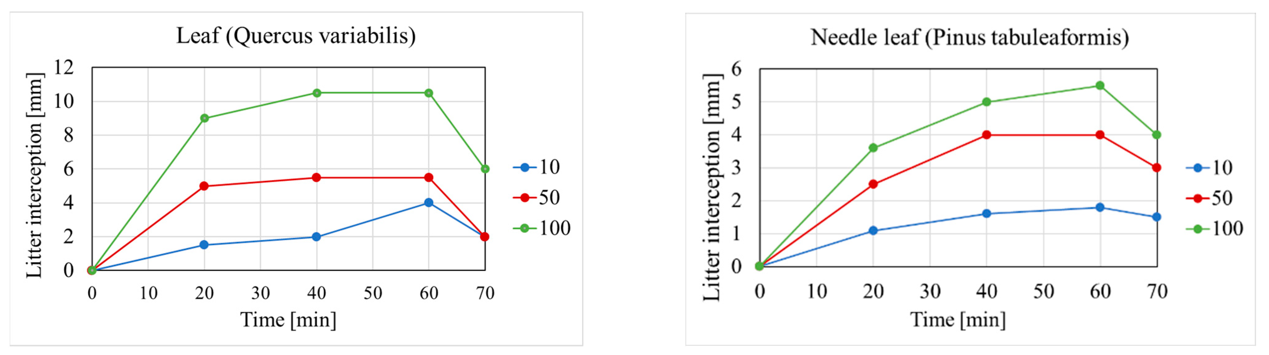
23] showed experimentally that the leaf litter storage changes with time, and storage capacity is greater for high rainfall intensity. In their work, they investigated the following woodland types:
Platycladus orientalis
Pinus tabulaeformis
Quercus variabilis
Acer truncatum
The Quercus variabilis and Pinus tabuleaformis tree varieties are similar to the Hungarian broadleaf and needle types. They performed experiments to measure leaf litter interception during a 60 min rainfall event using 10, 50, and 100 mm/h intensities. Their results for Q. variabilis and P. tabulaeformis appear in
Figure 9.
For 50 mm/h rainfall intensity, litter interception is constant after 40 min of rainfall for both leaf and needle leaf: 5.8 mm for leaf and 4 mm for needle leaf.
Kiss [
41] determined the release of stored water from the leaf litter. With Equation (3) below, 0.2–1.7 mm of interception can be determined on average for oak leaves; meanwhile, with beech and needle leaf types, around 3–4 mm of interception can be determined on average through a rainfall event. Equation (3) used an exponential draining process for three different leaf litter types:
where
w [mm] = the current water content of leaf litter,
wmin [mm] = the minimal water content,
Sa [mm] = the maximum storage capacity,
α′ [l/day] = the coefficient of the amount of the release of water content,
t′ [day] = elapsed time from the end of the rainfall.
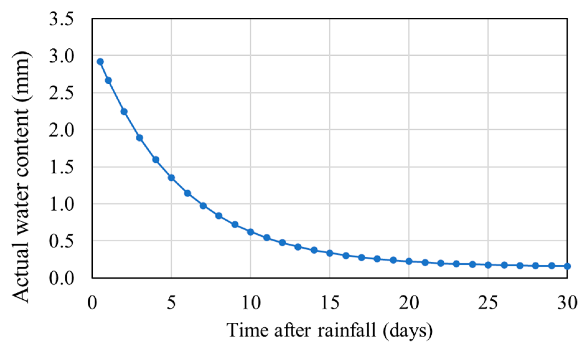
In the experiment, the collected samples were 0.75–1.25 kg/m
2, and the litter layer was around 1 cm thick. According to Kucsara and Gribovszki [
46], a leaf litter layer’s storage capacity grows with its thickness. The leaf litter releases its water rapidly in the first days, and then the release becomes slower (
Figure 10). According to the measurements [
41], the leaf litter has a sponge-like behavior. The water intake is fast, and the release is significantly slower. Therefore, laboratory experiments provided a more comprehensive picture of the leaf litter draining process. The experiment focused on the seasonal drainage in winter and summer. Based on experiments, the leaf litter drainage lasted 15–25 days.
5.2. Soil Infiltration
In this study, the Green and Ampt equations modeled the soil infiltration process [
47]. The 3D hydrosoil [
48] soil map provided estimates of the soil texture and hydraulic conductivity distribution in the Hidegvíz valley in the top 10 cm soil layer. The other soil parameters for the Green-Ampt equation were estimated based on the hydraulic conductivity, using values reported by Rawls et al. [
49].
5.3. Overland Flow Ratio
Watersheds with natural land cover have a significant variation in overland flow ratio (excess rainfall/total rainfall). Typical overland flow ratios used in Hungary for forested watersheds are 5–15%; meadows: 15–30% [
50].
For step-sloped watersheds, the ratio of overland flow can increase with increased intensity of rainfall [
51].
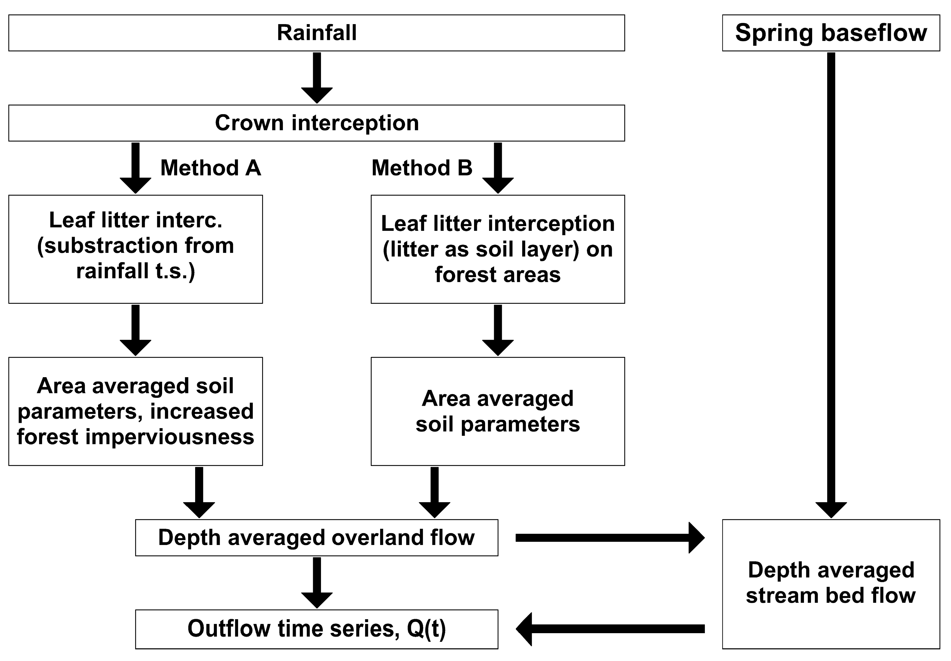
5.4. Modeling Approach
Two modeling approaches, Methods A and B, were developed and evaluated (
Figure 11). For Method A, canopy and leaf litter interceptions are subtracted from the rainfall time series. The remaining rainfall then infiltrates into the unsaturated soil layer. Excess rainfall generates overland flow:
where
heff [mm] = effective rainfall,
h [mm] = rainfall,
Ic [mm] = canopy interception,
Il [mm] = leaf litter interception,
Sd = depression storage, and
Fs [mm] = soil infiltration.
For Method B, only canopy interception is subtracted from rainfall. A pseudo-soil layer with high porosity and conductivity replaces the leaf litter, provides storage, and allows infiltration. The remaining excess rainfall generates overland flow:
where
heff [mm] = effective rainfall,
h [mm] = rainfall,
Ic [mm] = canopy interception,
Fl [mm] =litter infiltration,
Sd = depression storage, and
Fs [mm] = soil infiltration. The numerical model incorporated the two methods using the following approach.
The crown interception was calculated similarly in both models using Equation (1). Infiltration losses were calculated differently. Method A subtracted the leaf litter interception from the rainfall time series. The woodland areas were covered with leaf litter and assumed to be saturated and impervious throughout the simulation. Infiltration was calculated only in the remaining meadows (Brennbergi), lowlands, and stream beds (Magasbérci).
Method B modeled the leaf litter as a soil layer throughout the woodland area. The remaining meadow and lowlands consisted of Brennbergi and Magasbérci soils similar to Method A.
All the simulated events were about one day long, during which the leaf litter released perhaps 10% of its retained water [
41]. Therefore, the simulation did not consider water released from the litter. Excess rainfall resulted from subtracting canopy, leaf litter, and infiltration losses from rainfall. The hydrodynamic numerical model calculated overland flow based on excess rainfall. The selected two events allowed for model prediction and comparison between Methods A and B.
5.5. Governing Equations
The HEC-RAS model simulated surface runoff. The Finite Volume Method (FVM) used a 2D mesh to calculate overland flow. The most accurate solution is the complete hydrodynamical equation (shallow-water equations, SWE).
where
V [m/s] = velocity in x–y directions,
= gradient operator,
fc = Coriolis parameter,
k = unit vector in the vertical direction,
g [m/s
2] = gravity,
zs [m, mBf] = elevation of water surface,
h [m] = water depth,
vt [m
2/s] = horizontal eddy coefficient,
τb [N/m
2] = bed shear stress,
ρ [kg/m
3]= water density,
R [m] = hydraulic radius,
τsy [N/m
2] = wind shear stress on the water surface.
This study did not apply the wind shear stress factor. Due to its chaotic motion, turbulent mixing transfers the momentum between computational cells. In time-averaged velocity fields, dispersed mixing transfers momentum. Huang [
6] suggested that an additional turbulence model could simulate overland flow more accurately. With an additional eddy viscosity component, the size of the computation cells and the time step define the degree of numerical diffusion. The added eddies represent the flow more appropriately, producing more accurate results.
The Smagorinsky-Lilly turbulence model calculated the eddy viscosity by:
where
νS [m
2/s] = eddy viscosity,
D = matrix of dispersion coefficients,
u* [m/s] = averaged velocity around the stream bed,
h [m] = water depth in a cell,
Cs = Smagorinsky-coefficient (~0.005–0.2), Δ [m] = filter length (equal to the cell side length),
S [1/s] = temporal deformation vector
The modified SWE equation’s final form with the additional eddy viscosity model becomes:
The complete SWE method exhibited unstable behavior, even with the shortest possible time steps. Therefore, a simplified local inertia method (SWE-LIA) was adopted. The model’s stability increased by eliminating the nonlinear advection terms [
35]:
Almeida and Bates [
32] stated that the LIA method produces similar results to the SWE method when the Froude number is less than 0.5. Both methods (SWE and LIA) produced stable outputs during simulations of Event 2; therefore, the LIA method was adopted.
6. Numerical Grid Structure
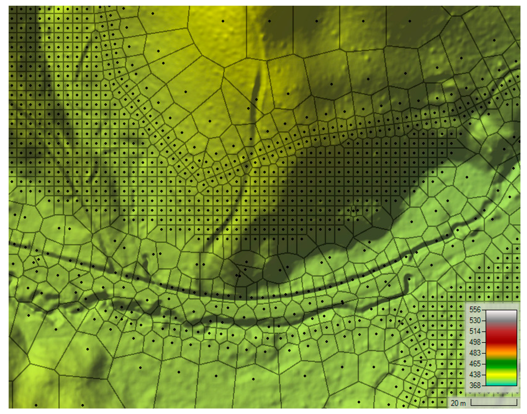
The calculation algorithm generated an adaptive mesh to discretize the watershed (
Figure 12). The mesh’s resolution depended on local geometrical parameters: where the effective overland flow ratio is high (creek beds, steep slopes, roads), the resolution is finer, while other areas did not need high resolution due to their high storage and slower flow velocity. The grid size ranged between 4 × 4 and 20 × 20.
The mesh’s resolution depends on the geometry of the terrain. The terrain types were divided into creek beds, steep slopes, and plain areas.
Creek beds: The steeper gradient necessitated the use of smaller cells. Accurate calculations in smaller creeks require the midpoints of the cells to be positioned within the bed. Otherwise, the calculations may introduce numerical errors from inappropriate mesh geometry in other areas.
Steep slopes: The model could quickly become unstable due to potential high velocities and corresponding Froude numbers. The average slope of the watershed areas is around 10%. Smaller cells improve the calculation’s stability.
Plain areas: The upland areas and areas around the bed creeks decline gently. The flow velocity decreases in these areas and does not require small cells.
The average time step of 0.4 s produced stable results.
7. Interception and Litter Storage Calculation
The crown interception was calculated for both methods using Equation (5). Crown storage capacity changes with different woodland types. The capacity varies from 1.5 to 4 mm and averages around 2–3 mm. During high-intensity rainfall, needle-type leaves can hold up to 6–8 mm [
46].
Method A calculated leaf litter storage for every time step of the measured rainfall data.
Table 2 lists input parameters for storage capacity. Calculating leaf litter storage on a watershed scale presented uncertainties due to variations in litter depth, area distribution through seasons, and its initial storage capacity before an event. The initial leaf litter storage was calculated based on the time after the preceding rainfall event. For Event 1, it was 20 days; for Event 2, it was 0.9 days.
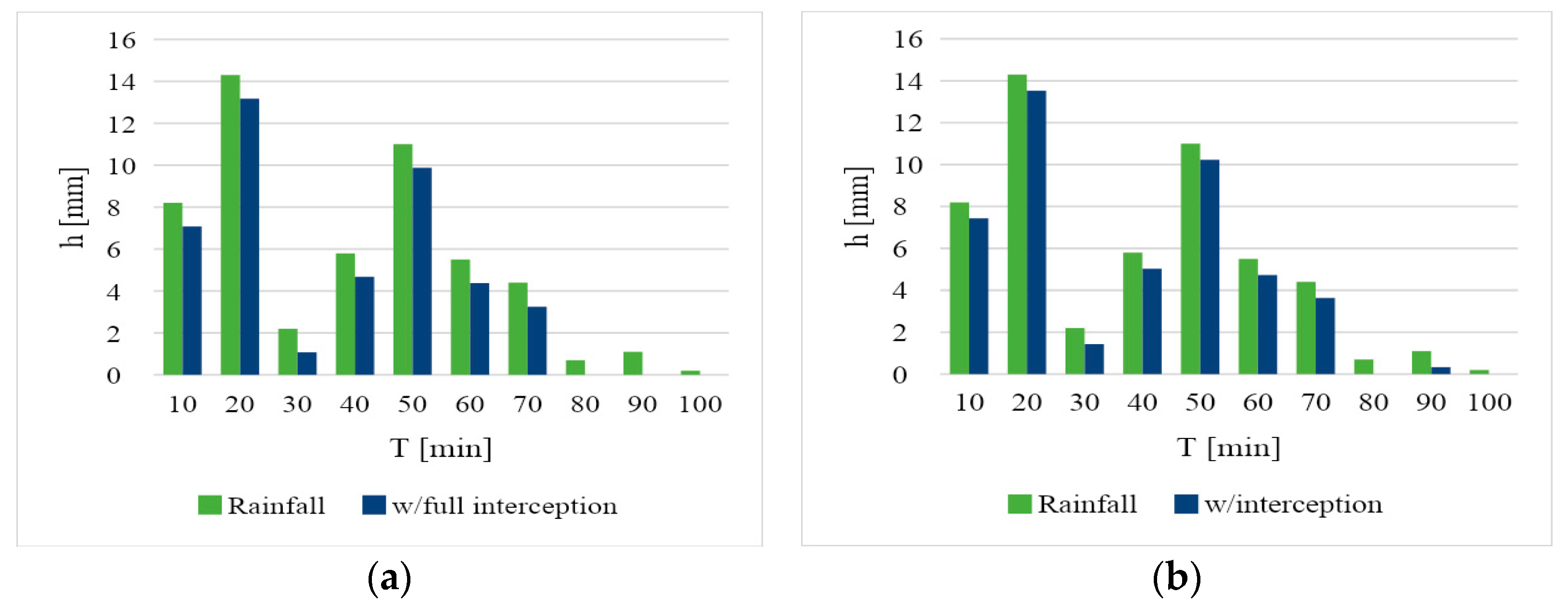
7.1. Event 1
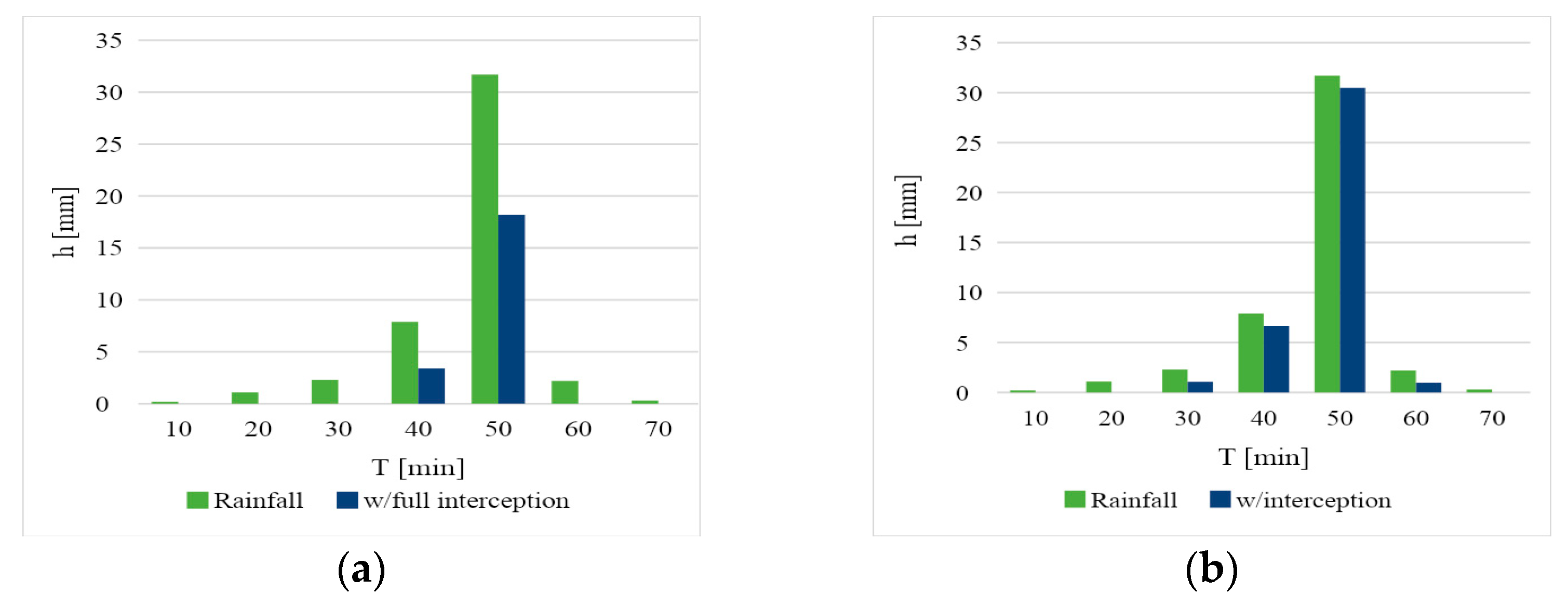
Time series interval: 15 July 2010 20:20–21:20, duration 70 min.
Figure 13a compares rainfall to effective rainfall after crown and leaf litter interception. It shows that only the highly intensive parts (20 min) of the rainfall reach the surface, creating overland flow and soil infiltration. Only the crown interception was subtracted in
Figure 13b. The effective rainfall time is 40 min, with slight rainfall loss.
The total rainfall volume was 271299 m3, the excess volume for Method A was 210,606 m3, and for Method B was 232,676 m3.
7.2. Event 2
Time series interval: 7 July 2012 14:40–16:50, duration 100 min.
Method A (
Figure 14a): The rainfall time series is 100 min long. By adding both crown and leaf litter interception, the length of the rainfall that reaches the surface was reduced to 70 min. In Method B (
Figure 14b), when only the crown interception is subtracted from the rainfall time series, the rainfall that effectively reaches the surface is 90 min.
The total rainfall volume was 317,011 m3, the excess volume for Method A was 258,324 m3, and for Method B was 275,188 m3.
8. Results
A comparison of results from Methods A and B follows in the next section. The discussion will first focus on the simulated discharge hydrographs at the watershed outlet for the two events. Then, the following sections discuss the difficulties and nuances of calibrating some parameters for the modeling process.
8.1. Soil Calibration Process
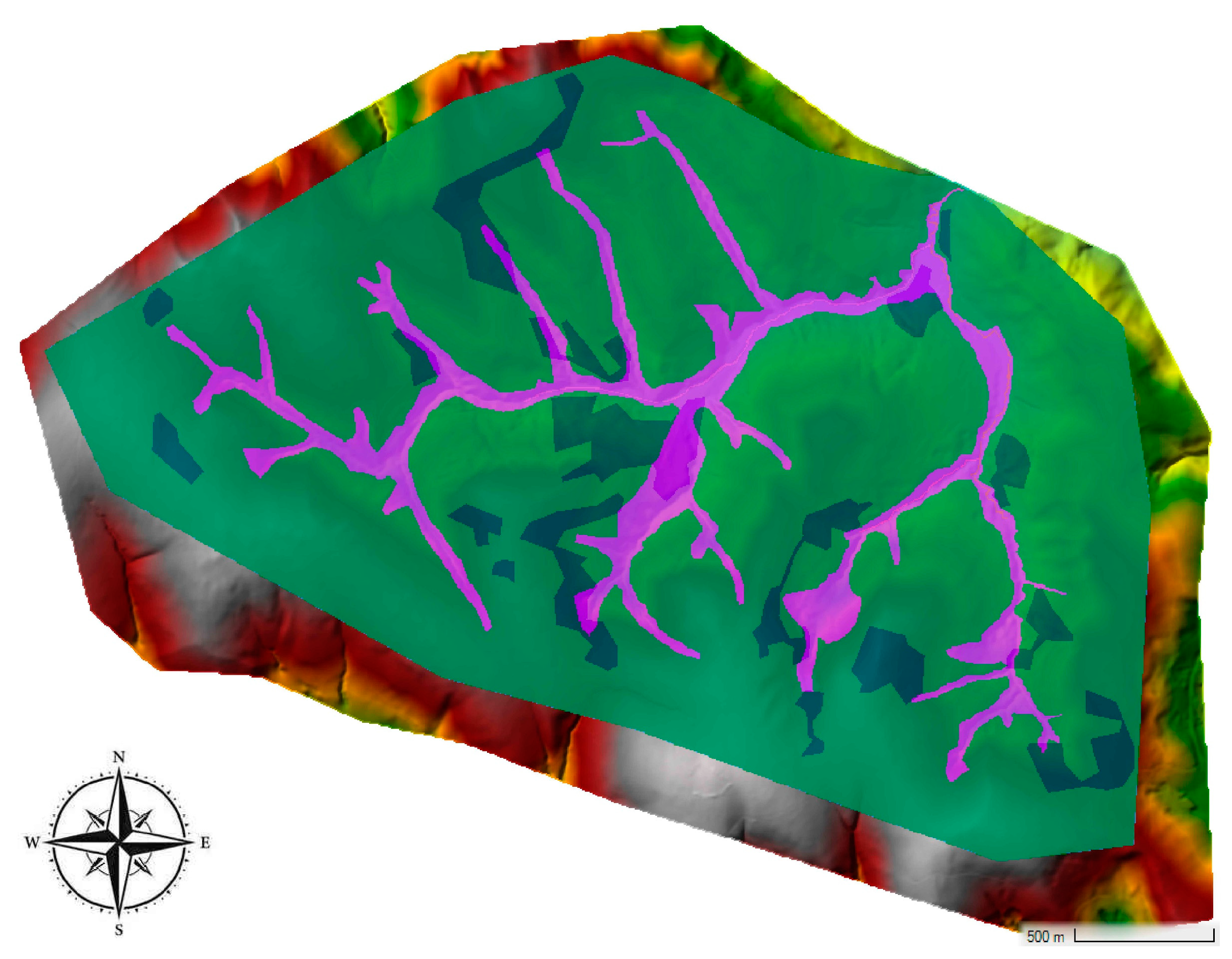
The calibration focused on determining soil parameters for the Hidegvíz Valley watershed. Analysis Method A required parameters for Bennberg and Magasberc soils that underlie the meadow and lowland (streambed) areas. Method B required a third pseudo-soil, the leaf litter, located in the woodland area.
Figure 15 shows the two meadowland/lowland soils with Magasberc in magenta and Breenberg in grey. Magasberc is prevalent along the streambeds and lowlands, while Breenberg is upland. The wooded area covers the majority of the valley in green. In order to distinguish between woodland and meadow areas, the land cover map was laid over the soil map. Where woodland areas were found (green), leaf litter was assumed and considered a soil layer or interceptor, as described earlier.
The woodland areas are the areas where leaf litter accumulates. Therefore, the focus during calibration was on this area. The calculation for Method A was as follows: In the woodlands, litter deficit is subtracted from the rainfall, and no further infiltration occurs (impervious). The rainfall in non-woodland areas interacts with the Magasberc or Brennberg surficial soils. The Green and Ampt equation determined the degree of infiltration. Green and Ampt parameters for the two soils were adjusted to produce reasonable behavior in the watershed.
The calculation for Method B was as follows: In the woodlands, a soil layer was approximated through leaf litter interception and storage using the Green and Ampt equations. In non-wooded areas, the same soils from Method A provided infiltration and runoff behavior.
The models required three steps for calibration. For Method A, the two events were evaluated, and parameters were adjusted until they reached optimal results. The interception and the leaf litter storage were subtracted from the rainfall time series and did not change during calibration. The soil parameters for the Green and Ampt equation were adjusted and remained the same for both events, except for initial water content. The final values appear in
Table 3.
In method B, where the leaf litter was approximated by soil, the two events were evaluated separately since the initial conditions of the litter were different. The soil parameters in the other regions (Brennberg and Magasberc) were identical to Method A.
Table 4 shows the modeled soil types with the selected parameters for the Green and Ampt equations.
The most recent rainfall before Event 1 occurred 20 days before, while for Event 2, rain occurred two days before. Therefore, the initial soil water contents for Event 2 were set at values higher than those set for Event 1. When a soil layer approximated the leaf litter, varying only the initial moisture content could not approximate the measured flow. The composition of the leaf litter was unknown, and its thickness may differ for the two events. The Green and Ampt equations could approximate leaf litter behavior, but it would require experimental determination since it does not behave like typical soil. During the evaluation, the leaf litter in the model was not sensitive to the initial water content; instead, the saturated hydraulic conductivity was the key. Earlier measurements showed similar scales in hydraulic conductivity [
52]. The saturated hydraulic conductivity was higher in Event 1 than in Event 2. The different conditions of the leaf litter, such as thickness, composition, and age, may explain this. Since several parameters interact and cannot be easily measured, the saturated hydraulic conductivity value might approximate the cumulative behavior.
The other parameter considered for calibration was the Manning
n number. The
n value depends on the structure of the surface. The overland flow’s depth is small; therefore, the shear stress has a higher impact on the flow; a rougher surface must be defined to approximate the surface roughness properly. For overland flow, Manning’s
n-values were assumed uniform during each event. The surface roughness was determined based on the land use distribution (
Figure 4) and applied based on literature values. During calibration, the
n values remained constant since the current HEC-RAS version only allows a linear change from an initial roughness to a final one. Possibly, if the roughness can vary nonlinearly throughout the simulation, the calibration would be more accurate. Manning’s
n-values are listed in
Table 5 for the four terrain types.
Method A assumed the forested areas were impervious, and the recommended n-value was applied to the forested surface. When a soil approximated the leaf litter (Method B), its effect on the overland flow differed. During the calibration, the overland flow on the leaf litter surface was smoother than on the natural forested surface; therefore, the forest area with litter received a smaller n-value.
8.2. Model Predictions
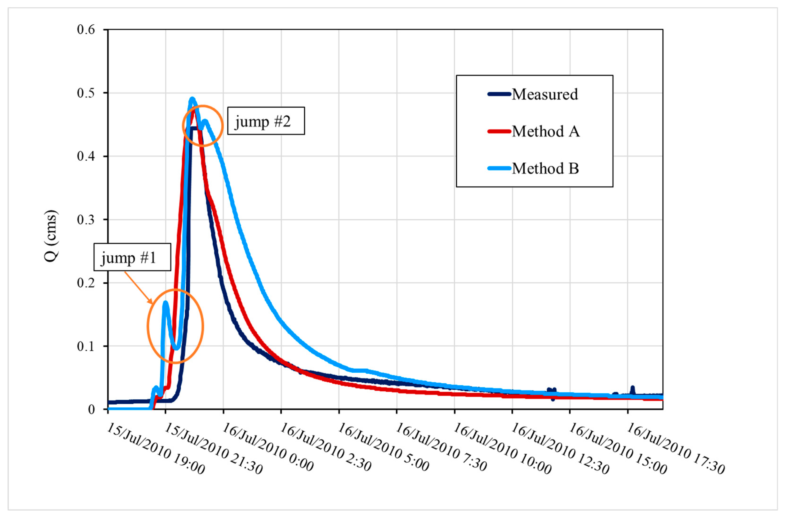
8.2.1. Event 1
Event 1 was modeled using Methods A and B. The results appear in
Figure 16. Using Method A, the peak flow and the recession limb followed the measured data well. Method B slightly overestimated the flow.
The time to peak of the modeled hydrographs is correct with both methods. There are jumps in the rising limb of the modeled hydrograph (Method B). Another jump occurs soon after the peak as well. Method B predicted a much more gradual recession than the measured flow.
Overprediction of overland flow velocities and volumes produced small jumps in the model hydrograph (
Figure 16). In Method B, when only the canopy interception is subtracted from the rainfall time series, the time of the concentration is shorter, and the runoff volume is greater than that in Method A. Due to the faster surface flow, runoff from the two small watersheds (Vadkan and Farkas Creek) arrived very quickly at the outlet, producing jump #1 in the numerical model. The modeled flow reduced after this peak for a short time until the flow from the larger, more dominant watershed (Rak Creek) arrived, and the flow increased again. The model accurately predicted the rising limb of the measured hydrograph after this time.
The second jump predicted by Method B comes from the overflows of the temporary ponding areas. This effect has also occurred during smaller flood events, as evidenced by flow measurements.
Method A estimated the measured hydrograph well. Also, in method A, the overland flow is slower due to the higher roughness of the forest area.
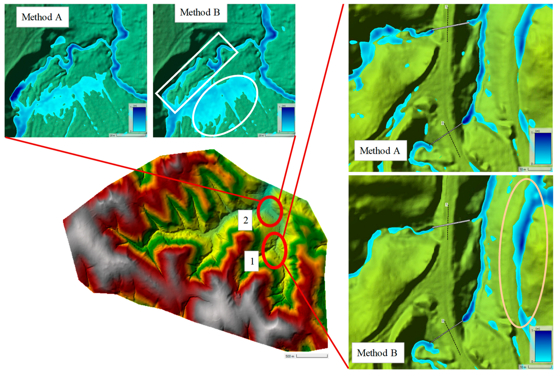
To illustrate the flow dynamics during Event 1, mainly when jump #1 occurs,
Figure 17 displays the spatial distribution of overland and channel flow depths. Method B exhibits a larger surface ponding area near the junction of Rák Creek (location 2, white circle) due to creek overflow. Channel flow (white rectangle) is smaller because the local peak flow has already moved downstream. In contrast, the creek channel is deeper in Method A because the surface runoff moves slower, allowing the creek to contain and convey the flow without breaching its banks. The difference originates from the choice of Manning’s n-values for Methods A and B, reflecting the differing surface roughness of soil and leaf litter, respectively. Method B allows faster overland flow due to the smoother leaf litter surface.
Near the Farkas and Vadkan culverts (location 1), both overland and creek flow depths are depicted for the upper region. Method B shows less water depth since the overland flow velocity is higher, indicating that the peak flow from these two smaller watersheds has passed this location. In local surface depressions, such as shown on the right side of the drainage system (orange circle), Method B accumulates more water in local storage since its more significant surface runoff has not yet infiltrated. The culverts across the road caused backwater effects along the stream since, in most cases, sediments fill the culverts and reduce flow. There was no information about the conditions of the culverts during the investigated events, so it was difficult to represent them accurately in the numerical model. In Method A, the average depth in the creek bed is lower, thus reducing the backwater effect at the culverts compared to Method B.
For Method B, recalibrating the culvert geometry may reduce jump #1 (
Figure 16) by simulating the effect of accumulated sediment. Since the actual conditions of the culverts were unknown, no further adjustments were attempted.
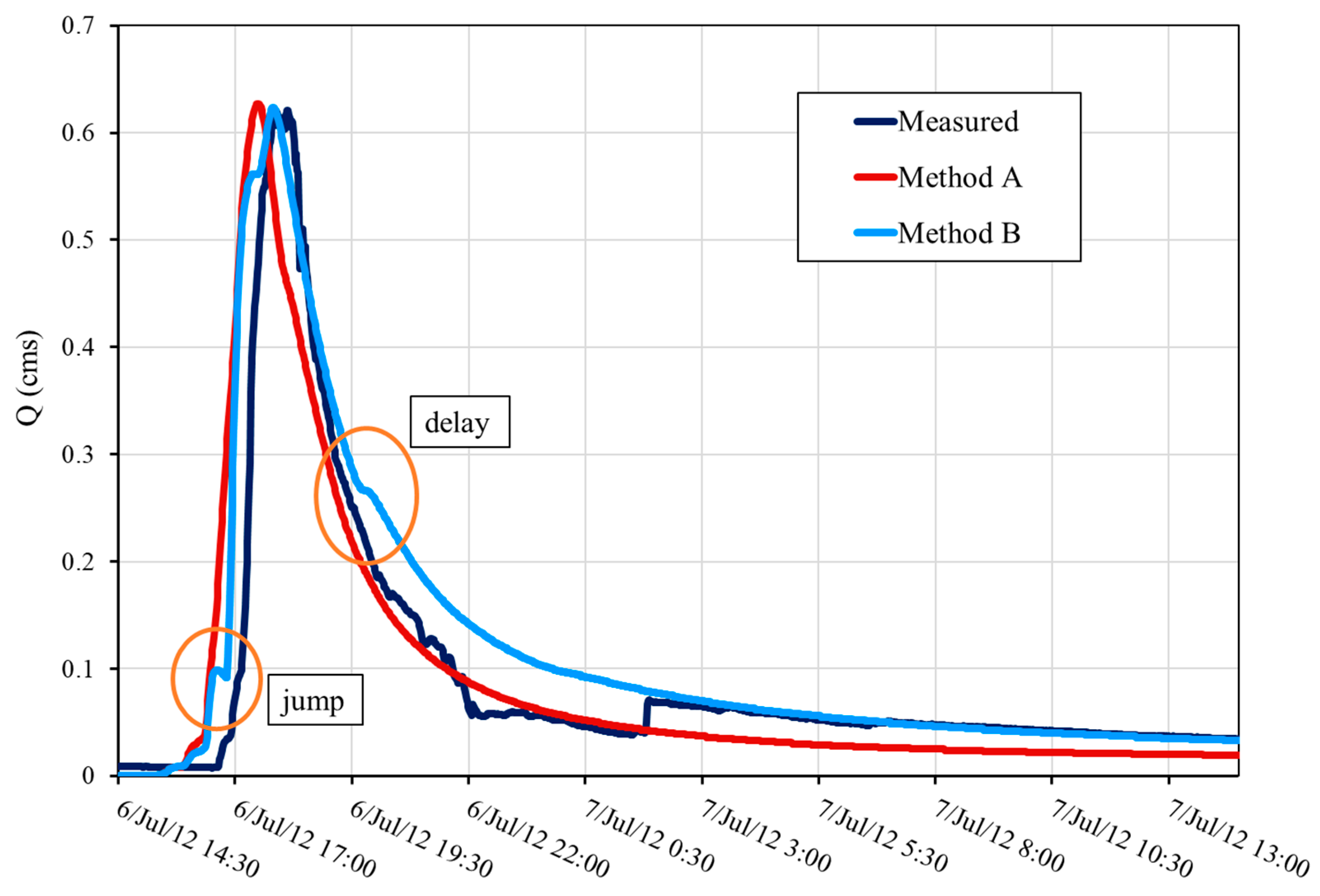
8.2.2. Event 2
Methods A and B showed promising results for Event 2, 7 June 2012 (
Figure 18). The predicted time of concentration, peak flow, and the recession limb agreed with the measured hydrograph. Method A slightly underestimated and Method B slightly overestimated peak flow.
Both methods modeled the shape of the rising limb, but they rose earlier than the measured hydrograph and reached their peak earlier than the measured value. Method B showed the same jump response in the rising limb, similar to Event 1, but to a much lesser degree. A small jump appears in the measured flow but is much less significant. As with Event 1, it comes from the faster time of concentration of the Farkas and Vadkan Creek watersheds.
Both of the methods overpredicted the flow velocity for the two smaller watersheds, but the modeled flow from Rák Creek appears to follow the measured hydrograph well. Both of the methods’ recession limbs are more gradual until their inflection points. After the inflection point, Method A reaches baseflow earlier and slightly underestimates it. With Method B, the flow slows slightly after the inflection point and then reduces to the measured flow, slightly overestimating it. The slight delay in the recession limb may result from the saturating leaf litter layer or numerical error. The numerical error originated from the constraints of the model itself. Throughout the modeling process, numerical sensitivity to the mesh and time steps increased in regions where steeper slopes transitioned to milder ones, particularly after reaching peak flow. Enhancing the average resolution of the cells mitigated these errors. However, reducing the time step beyond a specific threshold (0.1 s) was not feasible without introducing instability into the entire model. During modeling, larger excess rainfall contributed to stabilizing the model.
The adjusted model with Method B nicely fits into the baseflow curve after the jump in the measured hydrograph.
Table 6 shows the summary statistics of the calibrated models using Methods A and B. They both approximated peak flows well. Method B predicted the time to peak better than Method A for Event 2, where a soil layer defines the leaf litter. The volume error was unreliable since there was an error in the measurement on the recession limb of the hydrograph. Blockages in the weir could have produced the observed decrease in the measured data, perhaps driftwood or sediment accumulation. After 07.07, at 01:30, Method B fits the measured data better. If the measurement error is not considered, the decreasing limb of Method B fits better for the possible real flow time series. Therefore, the NSE value should be higher.
9. Conclusions
The present study focused on applying canopy interception and leaf litter retention in the hydrodynamic 2D modeling of a flash flood event in a small, forested watershed. Earlier models simulated flash flood events but did not include these components. Two modeling approaches were applied to study the influence of canopy and leaf litter on estimating surface runoff for two rainfall events.
Both models predicted runoff better for Event 2, where the runoff volume was larger, creating a greater depth in overland flow. The shallower depths from Event 1 tended to be less stable and less predictable. Unfortunately, these two events were the largest in the database. A higher-intensity event with substantial duration would have improved the prediction process.
Another significant challenge in the modeling process was the variability in the condition of leaf litter (such as its thickness and moisture content), which was greatly influenced by preceding rainfall events and prevailing meteorological conditions. This variability added a layer of complexity to the accurate prediction of the watershed’s response to rainfall events, particularly in establishing the initial conditions for each simulation. The leaf litter’s storage capacity was very sensitive to its condition, requiring a more meticulous reassessment before each event than ordinary soil conditions.
This study averaged soil and leaf litter parameters over the computational grid areas. However, increasing the refinement of the soil grid created additional instabilities in calculating surface runoff. The model’s sensitivity to the mesh and time steps, combined with the inherent limitations of the modeling software regarding time step adjustments, meant that any further increase in the resolution of the soil and leaf litter distribution reduced numerical stability. Employing area averaging for loss approximations in smaller watersheds could prove more effective in achieving accurate results.
This behavior also occurred for culvert structures within the model. The sensitivity of culverts’ parameters varied with the slope and length of the structure and had minimal impact on the outcomes. In contrast, modifications in the diameter, representing sediment accumulation inside the culvert, had a pronounced effect by creating backwater conditions.
Method A subtracted the canopy and leaf litter interceptions from the rainfall and assumed that the areas covered with leaf litter were impervious for the event duration. In Method B, leaf litter interception and storage processes were modeled as soil using the Green and Ampt equations. From the modeling, the following conclusions can be stated:
The linear formula based on woodland types estimates the crown interception to a reasonable degree of accuracy.
If the Green and Ampt soil parameters model is applied to the leaf litter calculations, then it must account for antecedent moisture conditions (saturation). Events 1 and 2 began with different initial moisture conditions in the leaf litter and underlying soil. Before either event, there was no information about the leaf litter’s thickness, current composition, or in situ moisture content.
The results also showed that predicting the decreasing limb had less error for the smaller rainfall event when the leaf litter was modeled as a soil layer (Method B).
For both events, Method A performed well. It was less sensitive to the initial conditions of the leaf litter, rainfall duration, and intensity.
The models showed that a 2D hydrodynamical model can be used to estimate the effect of leaf litter on a steep-sloped watershed. The calculation with both methods is more stable if the excess rainfall is higher. These results suggest that the accuracy improves with flash-flood events. Therefore, both methods may correctly model flash floods.
When leaf litter interception was subtracted from the rainfall time series, the leaf litter storage capacity was connected to the rainfall intensity. These subtractions were the basis for calculating the losses in Method A. Even a rudimentary estimate improves the modeling results. This method is ideal for ungauged watersheds, planning processes, or water damage prevention projects. During a rainfall event on an ungauged forested watershed, where the land use is known, leaf litter storage volumes can be predicted as a function of rainfall intensity. However, this method cannot calculate the saturation of the leaf litter. Therefore, it should be applied if measured data are available, or if the leaf litter layer is thick and mostly dry.
Method B is more precise than Method A for predicting the flow’s physical processes. Soil parameters can estimate the behavior of the leaf litter during a flash flood event since litter interception and storage in a short period work similarly to unsaturated soil. Of course, the behavior of leaf litter is not the same as that of the soil, but field or laboratory measurements can provide estimates. Since proper leaf litter data will not always be available for a given watershed, the modeling of the litter should depend on as few parameters as possible. This study found that hydraulic conductivity and the initial water content were the two most significant parameters.
The results showed that, during the modeling of the overland flow, the land use controls the time to peak and the slope of the rising and the recession limb. Compared with Method A, only crown interception modifies the rainfall time series. The process of surface storage calculation in this method is more complex, and the surface roughness is more accurate since the numerical model does not neglect leaf litter. Therefore, Method B’s complex physical model structure gives a more accurate simulation for predicting flood events in a forested watershed. Method B can be more accurate for ungauged watersheds since the land use and the vegetation type are the model’s key elements (in addition to a proper DEM).
This study applied a new approach to overland flow modeling compared to previous studies. Both crown and leaf litter interception significantly affect overland flow, although the conditions change with time. Therefore, combining complex overland flow simulation and substituting leaf litter with a soil layer can effectively predict flash floods in forested watersheds.
The main accomplishment of this study was in demonstrating the feasibility of constructing a model for steeply sloped, forested watersheds. Such watersheds, often situated in the upper reaches of larger catchments, are typically prone to high risks of flash flooding. Detailed and complex models are essential to understand the behavior of these types of watersheds. This study focused on integrating numerical solutions with empirical methods, illustrating how various available data can be utilized within a single model framework. The dual approach of numerical and empirical methods also lays the groundwork for comparative studies. Although the methodology for calculating overland flow remains consistent, the computation of losses varies, which is particularly valuable since many of these smaller watershed areas lack gauging stations. In ungauged watersheds, comparative modeling is a vital strategy for reducing uncertainties. Consequently, one of the aims of this study was to establish a foundation for modeling approaches that can be applied in planning processes, especially in ungauged watersheds with a significant risk of flash flooding.
Author Contributions
Conceptualization, G.Á., K.B. and R.R.; methodology, G.Á. and K.B.; software, G.Á.; validation, R.R. and Z.G.; formal analysis, G.Á.; investigation, G.Á., K.B., R.R. and Z.G.; resources, G.Á., R.R. and Z.G.; data curation, Z.G. and P.K.; writing—original draft preparation, G.Á.; writing—review and editing, K.B. and R.R.; visualization, G.Á. and R.R.; supervision, K.B.; project administration K.B. All authors have read and agreed to the published version of the manuscript.
Funding
This study is part of ongoing research entitled “Microscale influence on runoff”, supported by the National Research, Development, and Innovation Office (OTKA project grant number SNN143972) and the Slovenian Research and Innovation Agency (N2-0313). As a joint project, the TKP2021-NKTA-43 project also supported the preparation of this paper: TKP2021-NKTA-43 has been implemented with the support provided by the Ministry of Innovation and Technology of Hungary (successor: Ministry of Culture and Innovation of Hungary) from the National Research, Development, and Innovation Fund, financed under the TKP2021-NKTA funding scheme. Additional research presented in the article was carried out within the framework of the Széchenyi Plan Plus program with the support of the RRF 2.3.1 21 2022 00008 project.
Data Availability Statement
The data presented in this study are available on request from the corresponding author. The data are not publicly available due to current research and running data processes.
Conflicts of Interest
The authors declare no conflict of interest.
References
- Blöschl, G. Runoff Prediction in Ungauged Basins, Synthesis across Processes, Places and Scales. In Runoff Prediction in Ungauged Basins; Chapter: A Data Acquisition Framework for Predictions of Runoff in Ungauged Basins; Cambridge University Press: Cambridge, UK, 2013. [Google Scholar]
- Rana, V.K.; Suryanarayana, T.M.V. Estimation of flood influencing characteristics of watershed and their impact on flooding in data-scarce region. Ann. GIS 2021, 27, 397–418. [Google Scholar] [CrossRef]
- Garambois, P.A.; Larnier, K.; Roux, H.; Labat, D.; Dartus, D. Analysis of flash flood-triggering rainfall for a process-oriented hydrological model. Atmos. Res. 2013, 137, 14–24. [Google Scholar] [CrossRef]
- Hromadka, T.V.; Rao, P. Application of Diffusion Hydrodynamic Model for Overland Flows. Open J. Fluid Dyn. 2019, 9, 334–345. [Google Scholar] [CrossRef]
- Weinghuo, H.; He, H. Flood Forecasting Model Using the Combination Approach. Comput. Sci. IT Res. J. 2020, 1, 59–64. [Google Scholar] [CrossRef]
- Huang, W.; Cao, Z.-X.; Qi, W.-J.; Pender, G.; Zhao, K. Full 2D Hydrodynamic Modelling of Rainfall-induced Flash Floods. J. Mt. Sci. 2015, 12, 1203–1218. [Google Scholar] [CrossRef]
- Bizhanimanzar, M.; Leconte, R.; Nuth, M. Catchment-Scale Integrated Surface Water-Groundwater Hydrologic Modelling Using Conceptual and Physically Based Models: A Model Comparison Study. Water 2020, 12, 363. [Google Scholar] [CrossRef]
- Lago, C.A.F.; Giacomoni, M.H.; Bentivoglio, R.; Taormina, R.; Gomes, M.N.; Mendiondo, E.M. Generalizing rapid flood predictions to unseen urban catchments with conditional generative adversarial networks. J. Hydrol. 2023, 618, 129276. [Google Scholar] [CrossRef]
- Xia, X.; Liang, Q.; Ming, X.; Hou, J. An efficient and stable hydrodynamic model with novel source term discretization schemes for overland flow and flood simulations. Water Resour. Res. 2017, 53, 3730–3759. [Google Scholar] [CrossRef]
- Liao, Y.; Zhao, H.; Jiang, Z.; Li, J.; Li, X. Identifying the risk of urban nonpoint source pollution using an index model based on impervious-pervious spatial pattern. J. Clean. Prod. 2020, 288, 125619. [Google Scholar] [CrossRef]
- Schneidewind, U.; Schneidewind, U.; Vandersteen, G.; Joris, I.; Seuntjens, P.; Batelaan, O. Delineating groundwater-surface water interaction. Hydrol. Process. 2015, 30, 203–216. [Google Scholar] [CrossRef]
- Ámon, G.; Bene, K. Impact of different rainfall events on overland flow using a 2D hydrodynamical model on a steep-sloped watershed. In Proceedings of the EGU23-9179, Vienna, Austria, 24–28 April 2023. [Google Scholar] [CrossRef]
- Acharya1, S.; McLaughlin, D.; Kaplan, D.; Cohen, M.J. A proposed method for estimating interception from near-surface soil moisture response. Hydrol. Earth Syst. Sci. 2020, 24, 1859–1870. [Google Scholar] [CrossRef]
- Gribovszki, Z. Comparison of specific-yield estimates for calculating evapotranspiration from diurnal groundwater-level fluctuations. Hydrogeol. J. 2018, 26, 869–880. [Google Scholar] [CrossRef]
- Zagyvai-Kiss, K. Az Avarintercepció Vizsgálata a Soproni-Hegységben (Hungarian, an Examination of the Leaf Litter Interception in the Mountains of Sopron). Ph.D. Thesis, Pál Kitaibel Doctoral School of Environmental Sciences, University of West Hungary, Sopron, Hungary, 2014. [Google Scholar]
- Deng, W.; Zheng, X.; Xiao, S.; Chen, Q.; Gao, Y.; Zhang, L.; Huang, J.; Bai, T.; Xie, S.; Liu, Y. Effects of leaf type, litter mass and rainfall characteristics on theinterception storage capacity of leaf litter based on process simulation. J. Hydrol. 2023, 624, 129943. [Google Scholar] [CrossRef]
- Sato, Y.; Kumagai, T.; Kume, A.; Otsuki, K.; Ogawa, S. Experimental analysis of moisture dynamics of litter layers—The effects of rainfall conditions and leaf shapes. Hydrol. Process. 2004, 18, 3007–3018. [Google Scholar] [CrossRef]
- Putuhena, W.M.; Cordery, I. Estimation of interception capacity of forest floor. J. Hydrol. 1995, 180, 283–299. [Google Scholar] [CrossRef]
- Bulcuck, H.H.; Jewitt, G.P.W. Field data collection and analysis of canopy and litter interception in commercial forest plantations in the KwaZulu-Natal Midlands, South Africa. Hydrol. Earth Syst. Sci. 2012, 16, 3717–3728. [Google Scholar] [CrossRef]
- Zagyvai-Kiss, K.A.; Kalicz, P.; Szilágyi, J.; Gribovszki, Z. On the specific water holding capacity of litter for three forest ecosystems in the eastern foothills of the Alps. Agric. For. Meteorol. 2019, 278, 107656. [Google Scholar] [CrossRef]
- Urbanik, M.; Olejnik, J.; Miler, A.T.; Krysztofiak-Kaniewska, A.; Ziemblinska, K. Rainfall Interception for Sixty-Year-Old Pine Stand at the Tuczno Forest District. Infrastrukt. Ekol. Teren. Wiej. 2015, 2, 377–384. [Google Scholar] [CrossRef]
- Zhao, L.; Hou, R.; Fang, Q. Differences in interception storage capacities of undecomposed broadleaf and needle-leaf litter under simulated rainfall conditions. For. Ecol. Manag. 2019, 446, 135–142. [Google Scholar] [CrossRef]
- Li, Q.; Lee, Y.E.; Im, S. Characterizing the Interception Capacity of Floor Litter with Rainfall Simulation Experiments. Water 2020, 12, 3145. [Google Scholar] [CrossRef]
- Du, J.; Xie, S.; Xu, Y.; Xu, C.; Singh, V.P. Development and testing of a simple physically-based distributed rainfall-runoff model for storm runoff simulation in humid forested basins. J. Hydrol. 2006, 336, 334–346. [Google Scholar] [CrossRef]
- Kim, T.; Kim, J.; Lee, J.; Kim, H.S.; Park, J.; Im, S. Water Retention Capacity of Leaf Litter According to Field Lysimetry. Forests 2023, 14, 478. [Google Scholar] [CrossRef]
- Cheng, W.; Tie, L.; Zhou, S.; Hu, J.; Ouyang, S.; Huang, C. Effects of Soil Arthropods on Non-Leaf Litter Decomposition: A Meta-Analysis. Forests 2023, 14, 1557. [Google Scholar] [CrossRef]
- Kees, C.E.; Band, L.E.; Farthing, L.W. Effects of Dynamics on Hillslope Water Balance Models; North Carolina State University, Center for Research in Scientific Computation: Raleigh, NC, USA; pp. 27695–28205.
- Costabile, P.; Costanzo, C.; Ferraro, D.; Macchione, F.; Petaccia, G. Performance of the New HEC-RAS Version 5 for 2-D Hydrodynamic-Based Rainfall-Runoff Simulations at Basin Scale: Comparison with a State-of-the Art Model. Water 2020, 12, 2326. [Google Scholar] [CrossRef]
- Chen, L.; Young, M.H. Green-Ampt infiltration model for sloping surfaces. Water Resour. Res. 2006, 42, 1–9. [Google Scholar] [CrossRef]
- Tokunaga, T.K. Simplified Green-Ampt Model, Imbibition-Based Estimates of Permeability, and Implications for Leak-off in Hydraulic Fracturing. Water Resour. Res. 2020, 56, e2019WR026919. [Google Scholar] [CrossRef]
- Tzimopoulos, D. New Explicit Form of Green and Ampt Model for Cumulative Infiltration Estimation. Res. J. Env. Sci. 2020, 14, 30–41. [Google Scholar]
- Almeida, G.; Bates, P. Applicability of the local inertial approximation of the shallow water equations to flood modeling. Water Resour. Res. 2013, 49, 4833–4844. [Google Scholar] [CrossRef]
- Ballesteros, C.J.A.; Eguibar, M.; Bodoque, J.M.; Díez-Herrero, A.; Stoffel, M.; Gutiérrez-Pérez, I. Estimating flash flood discharge in an ungauged mountain catchment with 2D hydraulic models and dendrogeomorphic palaeostage indicators. Hydrol. Process. 2011, 25, 970–979. [Google Scholar] [CrossRef]
- Cea, L.; Garrido, M.; Puertas, J.; Jácome, A.; Del Río, H.; Suárez, J. Overland flow computations in urban and industrial catchments from direct precipitation data using a two-dimensional shallow water model. Water Sci. Technol. 2010, 62, 1998–2008. [Google Scholar] [CrossRef]
- Brunner, G.W. HEC-RAS, River Analysis System Hydraulic Reference Manual; US Army Corps of Engineers, Hydrologic Engineering Center: Davis, CA, USA, 2020. [Google Scholar]
- Zhao, J.; Liang, Q. Novel variable reconstruction and friction term discretisation schemes for hydrodynamic modelling of overland flow and surface water flooding. Adv. Water Resour. 2022, 163, 104187. [Google Scholar] [CrossRef]
- Ferro, V.; Guida, G. A theoretically-based overland flow resistance law for upland grassland habitats. Catena 2022, 210, 105863. [Google Scholar] [CrossRef]
- Szatmári, G.; Pásztor, L. Comparison of various uncertainty modelling approaches based on geostatistics and machine learning algorithms. Geoderma 2018, 337, 1329–1340. [Google Scholar] [CrossRef]
- Csafordi, P.; Eredics, A.; Gribovszki, Z.; Kalics, P.; Koppan, A.; Kucsara, M. Hidegvíz Valley Experimental Watershed; Department of Hydrology, Institute of Geomatics and Civil Engineering, Faculty of Forestry, University of West Hungary: Sopron, Hungary, 2012. [Google Scholar]
- Tímár, G.; Szmorad, F. Új adatok a Soproni-hegység flórájához, (Hungarain, New Data on the Flora of the Soproni Mountains), KITAIBELIA I. J. Pannonian Bot. 1996, 17–24, ISSN 2064-4507 (Online) ISSN 1219-9672 (Print). [Google Scholar]
- Kiss, K.A. Az Avarintercepció Vizsgálata a Soproni-Hegységben. Ph.D. Thesis, University of Sopron, Sopron, Hungary, 2012. [Google Scholar]
- Király, G.; Csapody, I.; Szmorad, F.; Tímár, G. A Soproni-hegység edényes flórája (Vascular Flora of the Sopron Hills). Flora Pannonica J. Phytogeogr. Taxon. 2004, 2, 1589–7788. (In Hungarian) [Google Scholar]
- Kárpáti, Z. Die Florengrenzen in der Umgebung von Sopron und Florendistrikt Laitaicum. Acta Bot. Hung. 1956, 2, 281–307. [Google Scholar]
- Vendel, M. Sopron Környékének Geológiája II. Rész: A Neogén és a Negyedkor üledékei Erdészeti Kísérletek. 1930, pp. 1–16. Available online: https://epa.oszk.hu/01600/01635/00221/pdf/EPA01635_foldtani_kozlony_1977_107_34_256-265.pdf (accessed on 19 February 2024).
- Kucsara, M.; Gribowszki, Z. Az Intercepció Vizsgálata és Számszerűsítése, Csapadékeseményhez Kötött Modellel,(Hungarian, Examination and Quantification of Rainfall Interception, with a Model Tied to a Rainfall Event) Research Report; University of Soprom: Sopron, Hungary, 2014. [Google Scholar]
- Feldman, A.D. Hydrologic Modeling System HEC-HMS; Technical References Manual; US Army Corps of Engineering, Hydrologic Engineering Center: Davis, CA, USA, 2000. [Google Scholar]
- Laborczi, A.; Szatmári, G.; Kaposi, A.D.; Pásztor, L. Comparison of soil texture maps synthetized from standard depth layers with directly compiled products. Geoderma 2018, 352, 360–372. [Google Scholar] [CrossRef]
- Rawls, W.J.; Brakensiek, D.L.; Saxton, K.E. Estimation of Soil Water Properties. Trans. ASAE 1982, 25, 1316–1320. [Google Scholar] [CrossRef]
- Jancsó, B.; Kaveczki, G.; Kóczán, G.; Laborczi TMarcell, K. Csapadékvíz-Gazdálkodás Tervezési Követelményei Laszlo Raum. Requirements of Rainwater-Resources Planning. 2019. Available online: https://mernokvagyok.hu/vizgazdalkodas/wp-content/uploads/sites/23/2022/05/Csapade%CC%81kvi%CC%81zgazda%CC%81lkoda%CC%81s-terveze%CC%81si-ko%CC%88vetelme%CC%81nyei_201-VVT.pdf (accessed on 19 February 2024). (In Hungarian).
- Ámon, G.; Bene, K. Rainfall Duration and Parameter Sensitivity on Flash-Flood at A Steep Watershed. Pollack Period 2023, 18, 54–59. [Google Scholar] [CrossRef]
- Orfánus, T.; Zvala, A.; Čierniková, M.; Stojkovová, D.; Nagy, V.; Dlapa, P. Peculiarities of Infiltration Measurements in Water-Repellent Forest Soil. Forests 2021, 12, 472. [Google Scholar] [CrossRef]
- Engman, E.T. Roughness Coefficients for Routing Surface Runoff. J. Irrig. Drain. Eng. 1986, 112, 39–53. [Google Scholar] [CrossRef]
Figure 1.
Forest rainfall–runoff process.
Figure 1.
Forest rainfall–runoff process.
Figure 2.
Rainfall–runoff processes.
Figure 2.
Rainfall–runoff processes.
Figure 3.
Location of the Hidegvíz Valley watershed.
Figure 3.
Location of the Hidegvíz Valley watershed.
Figure 4.
Land use distribution on the watershed.
Figure 4.
Land use distribution on the watershed.
Figure 5.
Distribution of near surface soil types.
Figure 5.
Distribution of near surface soil types.
Figure 6.
Event 1, between 15 and 16 July 2010.
Figure 6.
Event 1, between 15 and 16 July 2010.
Figure 7.
Event 2 between 6 and 7 July 2012.
Figure 7.
Event 2 between 6 and 7 July 2012.
Figure 8.
Flow event occurrence before Event 2.
Figure 8.
Flow event occurrence before Event 2.
Figure 9.
Leaf litter storage capacity for different leaf types on a 60-minute rainfall event with 10, 50, and 100 mm/h intensities.
Figure 9.
Leaf litter storage capacity for different leaf types on a 60-minute rainfall event with 10, 50, and 100 mm/h intensities.
Figure 10.
Leaf litter storage (mm) vs. time (day) [
46].
Figure 10.
Leaf litter storage (mm) vs. time (day) [
46].
Figure 11.
Modeling approaches.
Figure 11.
Modeling approaches.
Figure 12.
The adaptive grid mesh.
Figure 12.
The adaptive grid mesh.
Figure 13.
Event 1 effect of interceptions, Method A (a) and Method B (b).
Figure 13.
Event 1 effect of interceptions, Method A (a) and Method B (b).
Figure 14.
Event 2 effect of interceptions, Method A (a) and Method B (b).
Figure 14.
Event 2 effect of interceptions, Method A (a) and Method B (b).
Figure 15.
Modeled soils (green—woodland (leaf litter as soil); dark blue—Magasbérc soil (cutting areas); magenta—Brennberg soil (meadows, creeks)).
Figure 15.
Modeled soils (green—woodland (leaf litter as soil); dark blue—Magasbérc soil (cutting areas); magenta—Brennberg soil (meadows, creeks)).
Figure 16.
Prediction results for Event 1, for Methods A and B.
Figure 16.
Prediction results for Event 1, for Methods A and B.
Figure 17.
State of modeled overland flow at jump #1 in both methods around the culverts (location 1) and the lower Rák Creek junction area (location 2) during Event 1.
Figure 17.
State of modeled overland flow at jump #1 in both methods around the culverts (location 1) and the lower Rák Creek junction area (location 2) during Event 1.
Figure 18.
Prediction results for Event 2, for Methods A and B.
Figure 18.
Prediction results for Event 2, for Methods A and B.
Table 1.
Measured rainfall and outflow values for Events 1 and 2.
Table 1.
Measured rainfall and outflow values for Events 1 and 2.
| | imax (mm/h) | iavg
(mm/h) | Rainfall
Duration
(min) | tc
(min) | Rainfall Volume
(m3) | Flow Volume
(m3) | Ratio |
|---|
Event 1
2010 | 190.2 | 35.6 | 70 | 170 | 276,438 | 5257 | 1.90% |
Event 2
2012 | 85.5 | 45.7 | 100 | 210 | 318,052 | 8133 | 2.56% |
Table 2.
Antecedent water content in the leaf litter for both events (Equation (3)).
Table 2.
Antecedent water content in the leaf litter for both events (Equation (3)).
| | t′ [day] | Sa [mm] | wmin [mm] | a’ | w [mm] |
|---|
| Event 1 | 20 | 3.184 | 0.147 | −0.185 | 0.22 |
| Event 2 | 0.9 | 3.184 | 0.147 | −0.185 | 2.72 |
Table 3.
Calibrated soil parameters.
Table 3.
Calibrated soil parameters.
| Soil Type | Sf [mm] | K [mm/h] | Initial Soil Water Content | Saturated Soil Water Content | Residual Soil Water Content | Pore Size Distribution Index |
|---|
| Magasberc | 261.76 | 15.67 | 0.20 | 0.33 | 0.04 | 0.35 |
| Brennberg, cutting areas | 219.04 | 26.67 | 0.18 | 0.35 | 0.03 | 0.40 |
Table 4.
Calibrated soil parameters with the added pseudo-soil of the leaf litter layer.
Table 4.
Calibrated soil parameters with the added pseudo-soil of the leaf litter layer.
| Area Type | Wetting Front Suction
Sf [mm] | Ksat [mm/h] | Initial Soil Water Content (-) | Saturated Soil Water Content (-) | Residual Soil Water Content (-) | Pore Size Distribution Index (-) |
|---|
| Magasberc soil (loam–sandy loam)—orange |
| Meadows areas, streambed | 261.76 | 15.67 | 0.20 | 0.33 | 0.04 | 0.35 |
| Brennberg soil (loamy sand–sandy loam)—grey |
| Meadow areas- | 219.04 | 26.67 | 0.18 | 0.35 | 0.03 | 0.40 |
| Leaf litter (loamy sand)—green, event 1 |
| Woodland areas | 134.24 | 115 | 0.13 | 0.41 | 0.02 | 0.56 |
| Leaf litter (loamy sand)—green, event 2 |
| Woodland areas | 20 | 63 | 0.38 | 0.41 | 0.02 | 0.56 |
Table 5.
Calibrated Manning’s n-values.
Table 5.
Calibrated Manning’s n-values.
| Terrain Type | Applied
Manning’s n-Value |
|---|
| Creek bed | 0.03 |
| Cutting area | 0.1 |
| Forest | 0.4 |
| Forest covered with leaf litter | 0.2 |
Table 6.
Statistics of the model results for both methods.
Table 6.
Statistics of the model results for both methods.
| | | Peak Flow [cms] | Time
to Peak
[hr] | NSE
(-) | Volume
Error (-) |
|---|
Event 1
15 July 2010 | Measured | 0.44 | 2.47 | | |
| Method A | 0.48 | 2.42 | 0.72 | 0.11 |
| Method B | 0.49 | 2.33 | 0.43 | 0.51 |
Event 2
7 June 2012 | Measured | 0.62 | 2.95 | | |
| Method A | 0.62 | 2.37 | 0.74 | 0.05 |
| Method B | 0.62 | 2.67 | 0.81 | 0.25 |
| Disclaimer/Publisher’s Note: The statements, opinions and data contained in all publications are solely those of the individual author(s) and contributor(s) and not of MDPI and/or the editor(s). MDPI and/or the editor(s) disclaim responsibility for any injury to people or property resulting from any ideas, methods, instructions or products referred to in the content. |
© 2024 by the authors. Licensee MDPI, Basel, Switzerland. This article is an open access article distributed under the terms and conditions of the Creative Commons Attribution (CC BY) license (https://creativecommons.org/licenses/by/4.0/).


