Figure 1.
(a) Topographical map of Bangladesh indicating the Sangu River basin; (b) topography of Sangu River basin; (c) land use in the basin; (d) demarcation of rain-gauge and discharge station in the basin.
Figure 1.
(a) Topographical map of Bangladesh indicating the Sangu River basin; (b) topography of Sangu River basin; (c) land use in the basin; (d) demarcation of rain-gauge and discharge station in the basin.
Figure 2.
Methodology of the study.
Figure 2.
Methodology of the study.
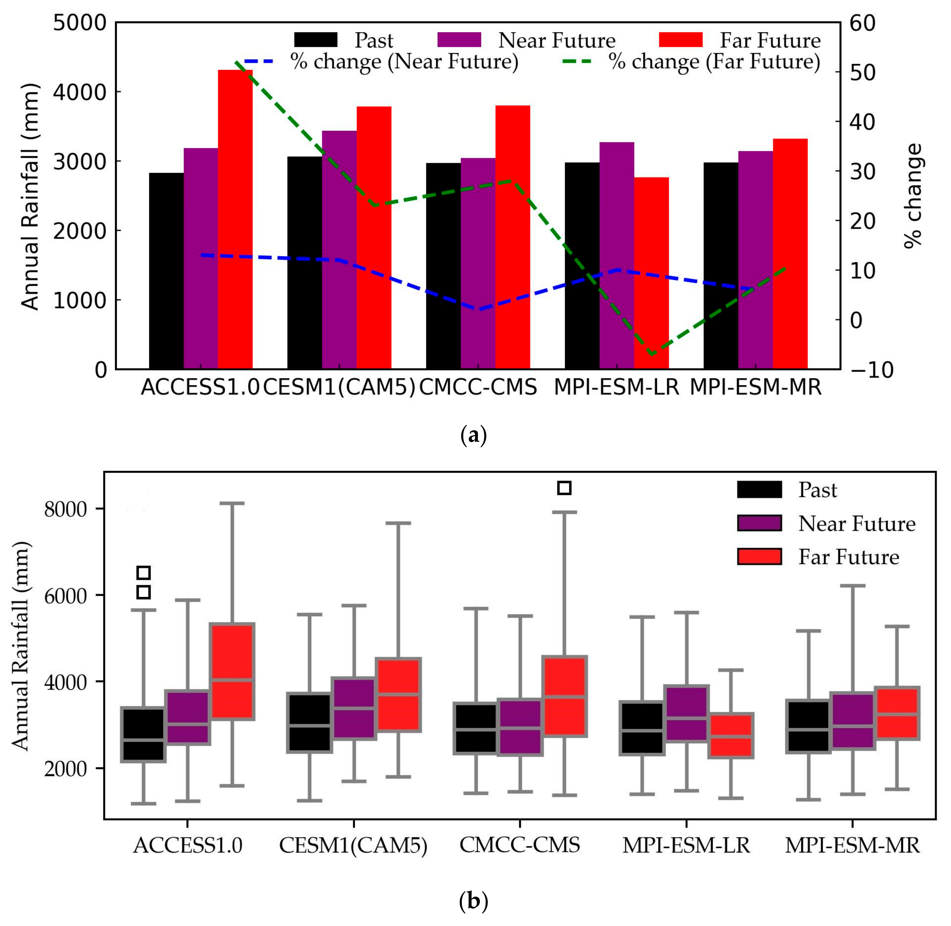
Figure 3.
(a) Comparison of basin average annual rainfall among the past, near-future, and far future, and percentage change for both the near-future and far-future. (b) Box and Whiskers of annual rainfall of each GCMs for the past, near-future, and far-future. Outliers beyond ±2 times the interquartile range are shown by black squares.
Figure 4.
Comparison of monthly rainfall among the past, near-future, and far-future. The solid line (past), dashed line (near-future), and dotted line (far-future) show the mean monthly rainfall, and the shaded area is the 95th and 5th percentiles of monthly rainfall.
Figure 4.
Comparison of monthly rainfall among the past, near-future, and far-future. The solid line (past), dashed line (near-future), and dotted line (far-future) show the mean monthly rainfall, and the shaded area is the 95th and 5th percentiles of monthly rainfall.
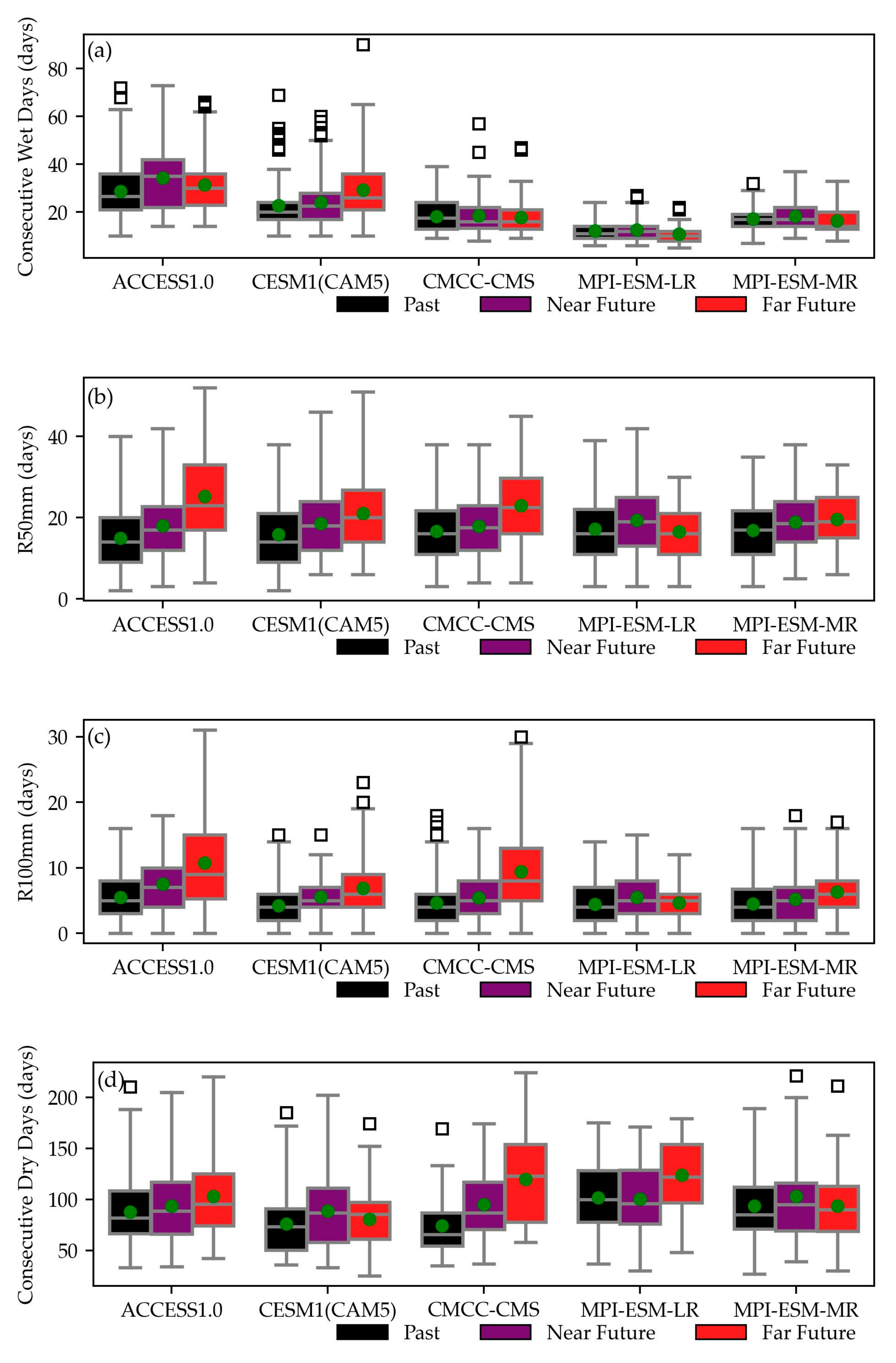
Figure 5.
Box–whisker plot for (a) consecutive wet days (CWDs), (b) R50mm, (c) R100mm, and (d) consecutive dry days (CDDs). Green circles show the mean value. Outliers beyond ±2 times the interquartile range are shown by black squares.
Figure 5.
Box–whisker plot for (a) consecutive wet days (CWDs), (b) R50mm, (c) R100mm, and (d) consecutive dry days (CDDs). Green circles show the mean value. Outliers beyond ±2 times the interquartile range are shown by black squares.
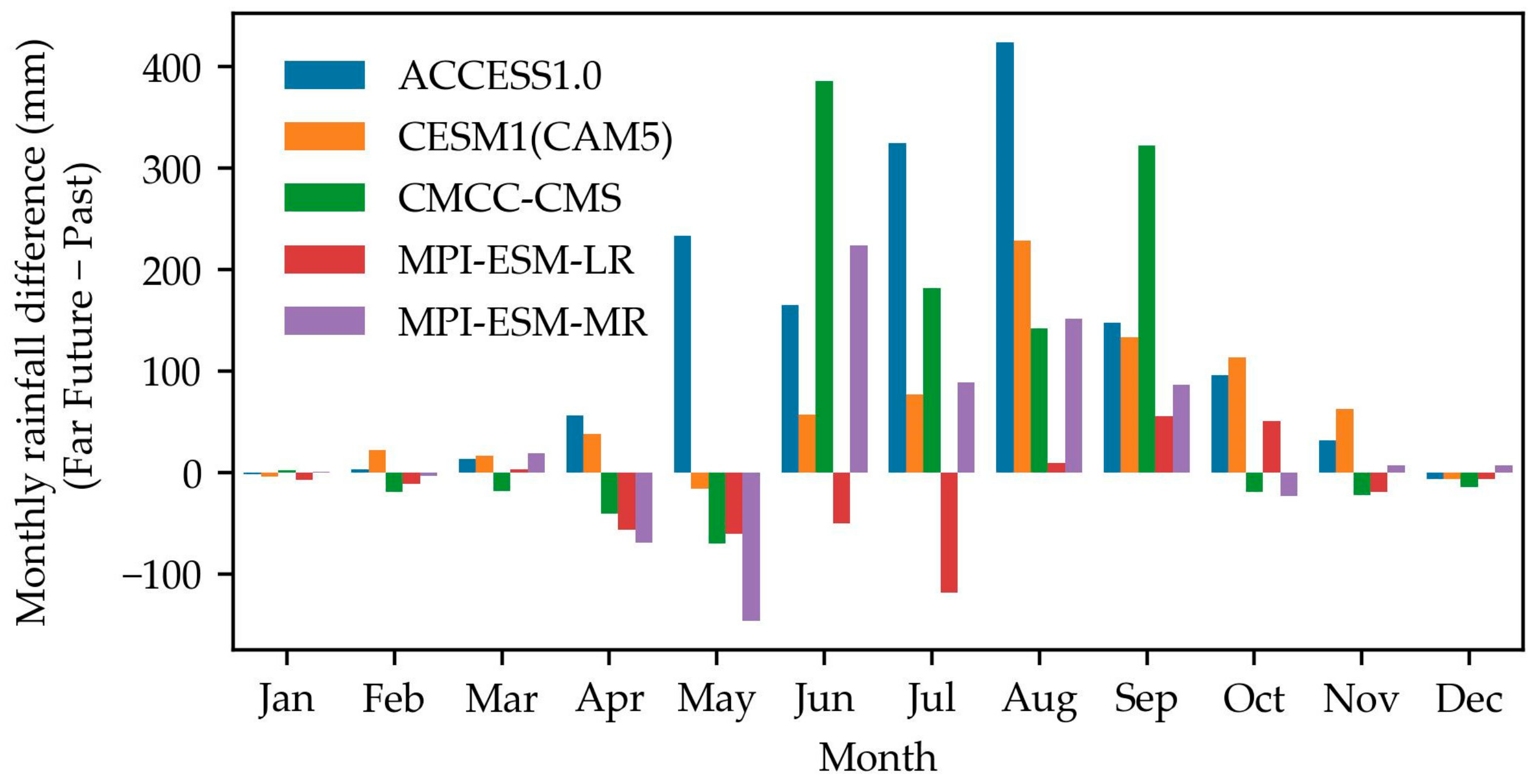
Figure 6.
Monthly rainfall difference (far-future minus past) of the selected GCMs.
Figure 6.
Monthly rainfall difference (far-future minus past) of the selected GCMs.
Figure 7.
Wind speed ratio (far-future divided by past) for the month of June. (a) ACCESS1.0, (b) CESM1(CAM5), (c) CMCC-CMS, (d) MPI-ESM-LR, (e) MPI-ESM-MR. Study area is located within the black box. Arrows are wind direction.
Figure 7.
Wind speed ratio (far-future divided by past) for the month of June. (a) ACCESS1.0, (b) CESM1(CAM5), (c) CMCC-CMS, (d) MPI-ESM-LR, (e) MPI-ESM-MR. Study area is located within the black box. Arrows are wind direction.
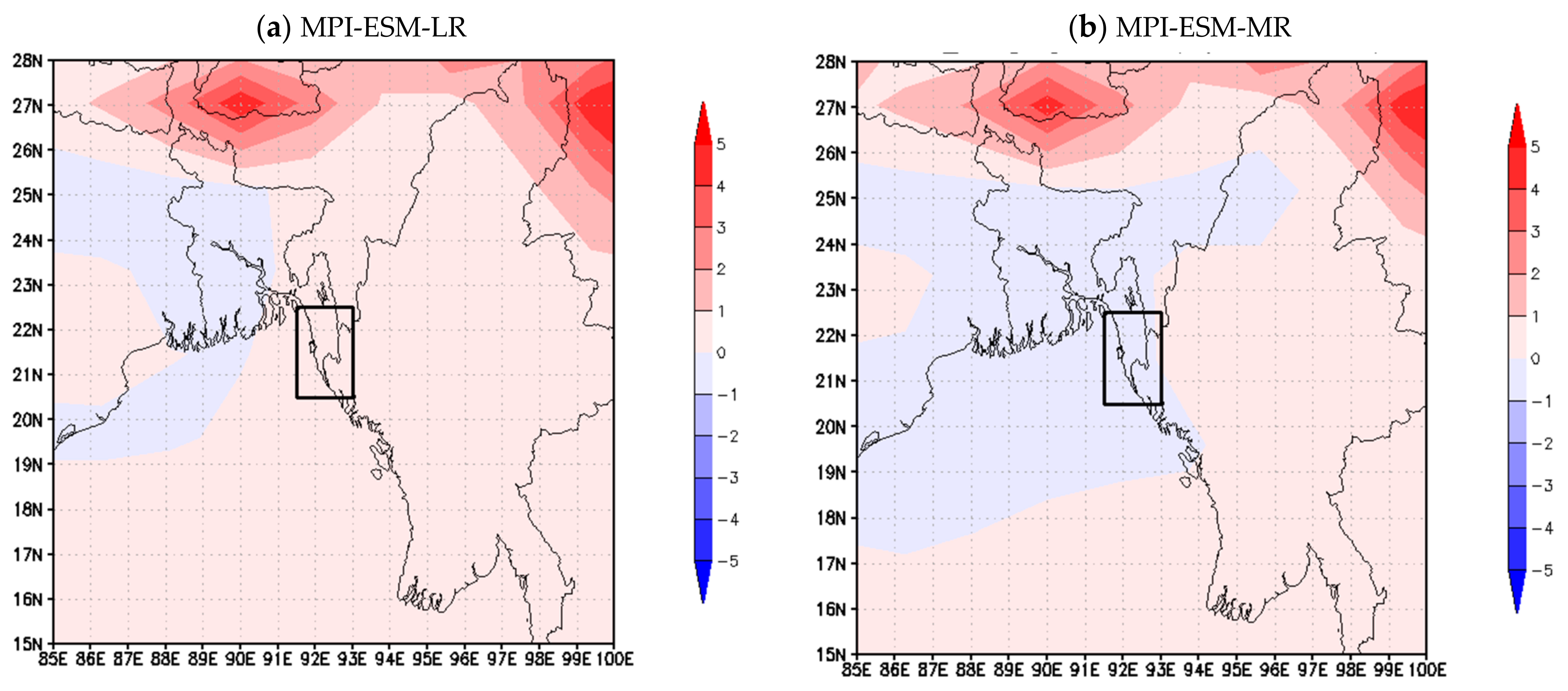
Figure 8.
Pressure difference (far-future minus past) for the month of July. (a) MPI-ESM-LR, (b) MPI-ESM-MR. Study area is located within the black box.
Figure 8.
Pressure difference (far-future minus past) for the month of July. (a) MPI-ESM-LR, (b) MPI-ESM-MR. Study area is located within the black box.
Figure 9.
Comparison between observed discharge and simulated discharge (a) model calibration for 1992–1993, and (b) model validation for 1997–2005.
Figure 9.
Comparison between observed discharge and simulated discharge (a) model calibration for 1992–1993, and (b) model validation for 1997–2005.
Figure 10.
Comparison of flood inundation in the Sangu River basin for the flood of 2015: (a) WEB-RRI simulated inundation; (b) MLSWI using MODIS data; (c) WEB-RRI simulated inundation depth (m).
Figure 10.
Comparison of flood inundation in the Sangu River basin for the flood of 2015: (a) WEB-RRI simulated inundation; (b) MLSWI using MODIS data; (c) WEB-RRI simulated inundation depth (m).
Figure 11.
Comparison between basin-averaged WEB-RRI ET and MODIS ET from the year 2009 to 2016.
Figure 11.
Comparison between basin-averaged WEB-RRI ET and MODIS ET from the year 2009 to 2016.
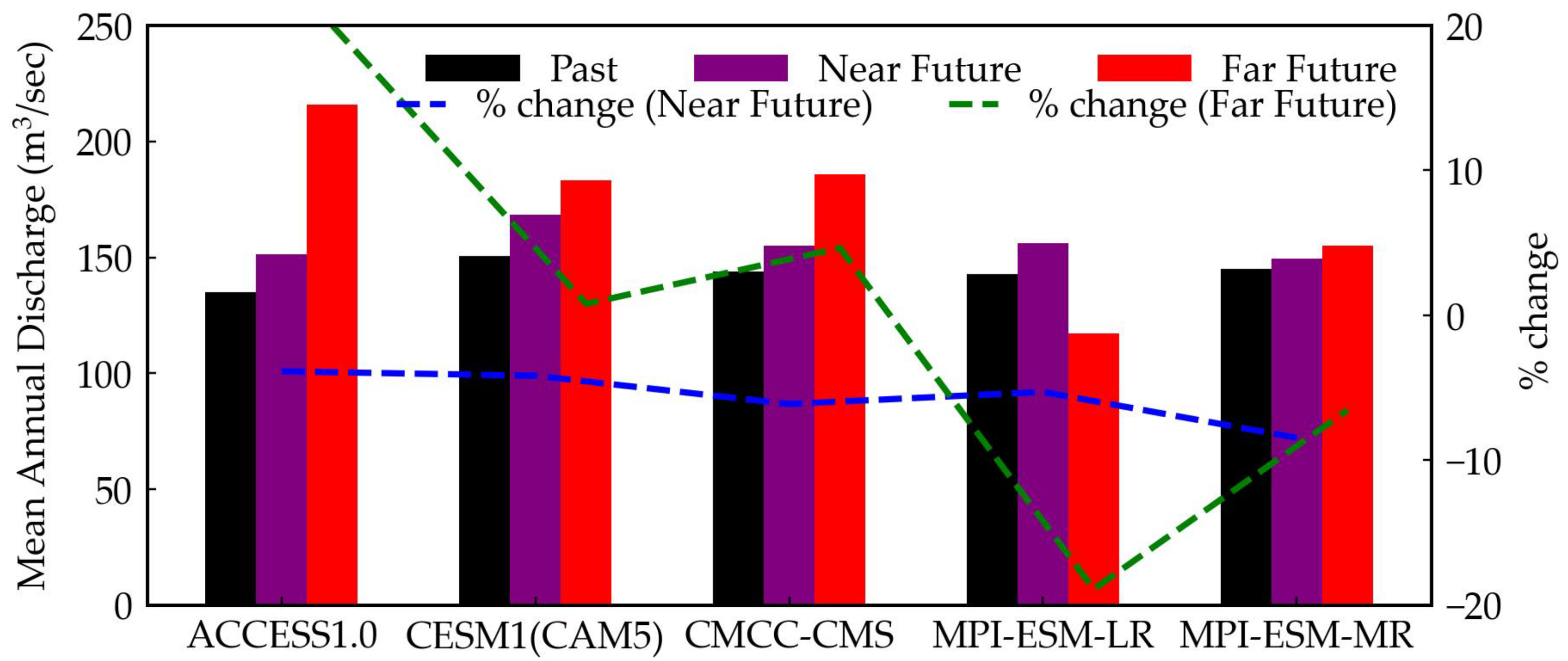
Figure 12.
Comparison of mean annual discharge among the past, near-future, and far-future, and percentage change for both the near-future and far-future.
Figure 12.
Comparison of mean annual discharge among the past, near-future, and far-future, and percentage change for both the near-future and far-future.
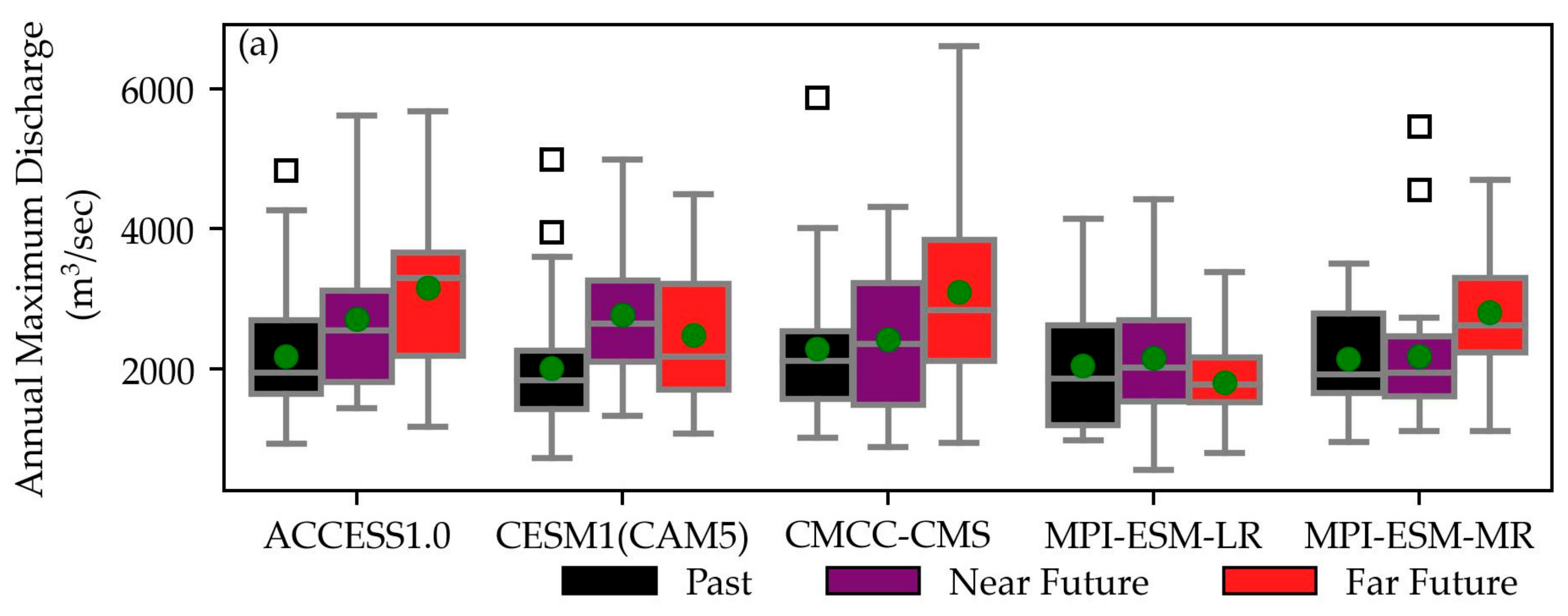
Figure 13.
Box and Whiskers of (a) annual daily maximum discharge and (b) annual daily minimum discharge at the Bandarban gauging station for the selected GCMs. Green circles show the mean value. Outliers beyond ±2 times the interquartile range are shown by black squares.
Figure 13.
Box and Whiskers of (a) annual daily maximum discharge and (b) annual daily minimum discharge at the Bandarban gauging station for the selected GCMs. Green circles show the mean value. Outliers beyond ±2 times the interquartile range are shown by black squares.
Figure 14.
Comparison of monthly discharge among the past, near-future, and far-future. The solid line (past), dashed line (near-future) and dotted line (far-future) show the mean monthly discharge, and the shaded area is the 95th and 5th percentiles of monthly discharge.
Figure 14.
Comparison of monthly discharge among the past, near-future, and far-future. The solid line (past), dashed line (near-future) and dotted line (far-future) show the mean monthly discharge, and the shaded area is the 95th and 5th percentiles of monthly discharge.
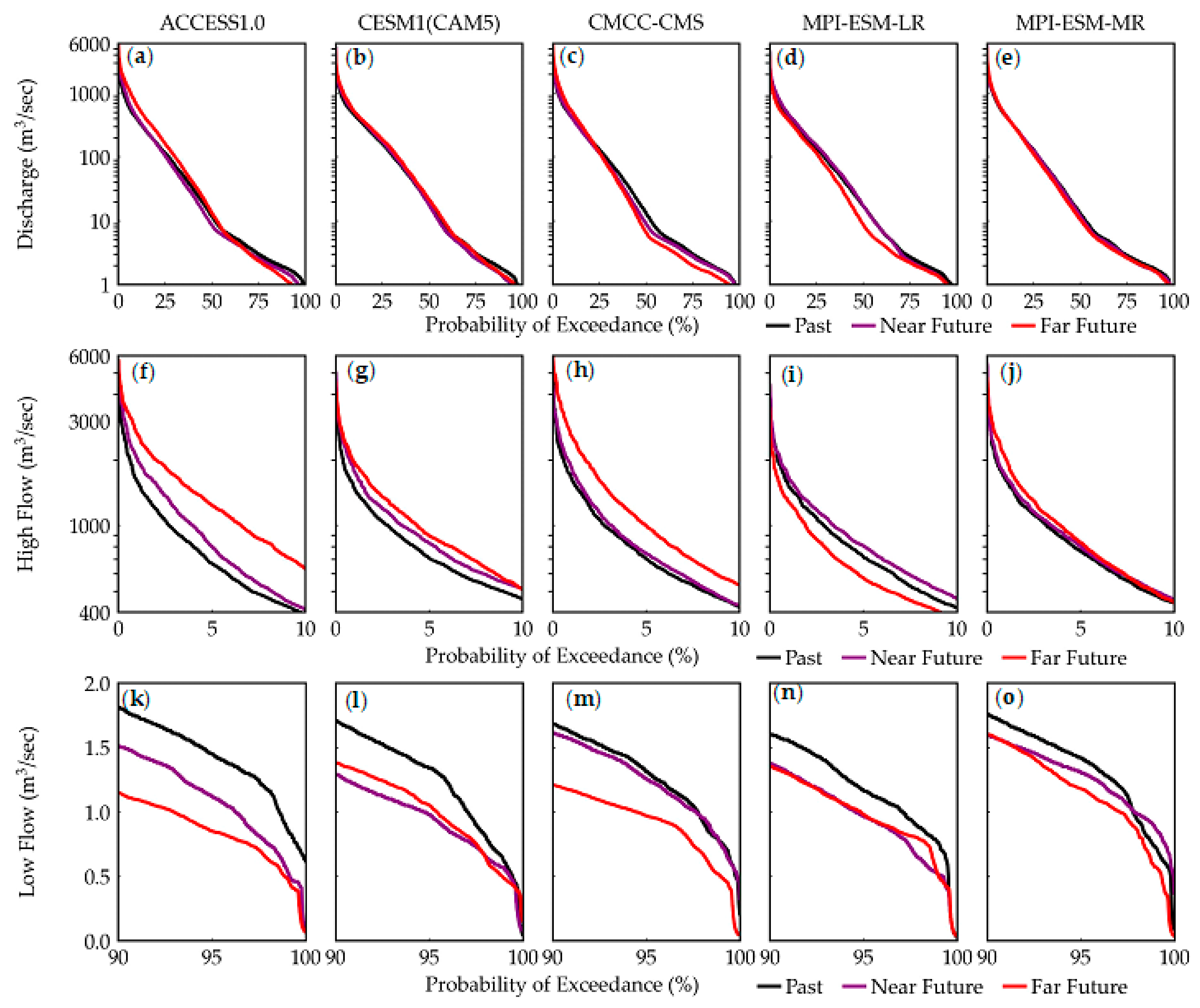
Figure 15.
Flow duration curve for the past, near-future, and far-future. (a–e) Entire period, (f–j) high flows (probability of exceedance ≤ 10%), and (k–o) low flows (90% ≤ probability of exceedance ≤ 100%).
Figure 15.
Flow duration curve for the past, near-future, and far-future. (a–e) Entire period, (f–j) high flows (probability of exceedance ≤ 10%), and (k–o) low flows (90% ≤ probability of exceedance ≤ 100%).
Figure 16.
All-time maximum inundation depth difference; (a–e) near-future minus past and (f–j) far-future minus past.
Figure 16.
All-time maximum inundation depth difference; (a–e) near-future minus past and (f–j) far-future minus past.
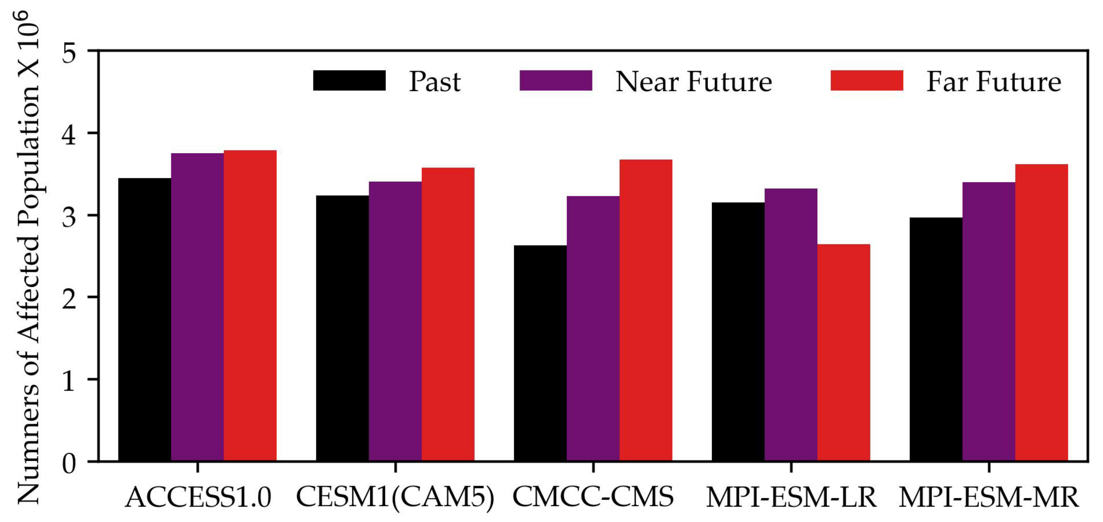
Figure 17.
Number of affected people in the Sangu River basin in the past, near-future, and far-future for all selected GCMs.
Figure 17.
Number of affected people in the Sangu River basin in the past, near-future, and far-future for all selected GCMs.
Figure 18.
Monthly ET for the all selected GCMs in the past, near-future, and far-future.
Figure 18.
Monthly ET for the all selected GCMs in the past, near-future, and far-future.
Figure 19.
Monthly transpiration for all selected GCMs in the past, near-future, and far-future.
Figure 19.
Monthly transpiration for all selected GCMs in the past, near-future, and far-future.
Table 1.
Extreme rainfall indices.
Table 1.
Extreme rainfall indices.
| Index | Descriptive Name | Definition | Unit |
|---|
| CWD | Consecutive wet days | Maximum number of consecutive rainy days with rainfall ≥ 1 mm | Days |
| CDD | Consecutive dry days | Maximum number of consecutive days with rainfall < 1 mm | Days |
| Rnn * | Number of days above nn | Yearly number of days with rainfall ≥ nn (nn is a user-defined threshold) | Days |
Table 2.
Model selection summary.
Table 2.
Model selection summary.
| Model Name | Institute | Country | Precipitation | Total Index | Remarks |
|---|
| ACCESS1.0 | CSIRO-BOM | Australia | 1 | 6 | Selected |
| CESM1(CAM5) | NCAR | USA | 1 | 8 | Selected |
| CMCC-CMS | CMCC | Italy | 1 | 7 | Selected |
| CNRM-CM5 | NCMR | France | 0 | 6 | PPR 1 |
| GFDL-CM2.1 | NOAA-GFDL | USA | 1 | 6 | NFD 2 |
| MPI-ESM-LR | MPI-N | Germany | 1 | 7 | Selected |
| MPI-ESM-MR | MPI-N | Germany | 1 | 6 | Selected |
| MPI-ESM-P | MPI-N | Germany | 1 | 7 | NFD 2 |
Table 3.
Daily rain-gauges in the Sangu River basin with ID, name, location, and average annual rainfall.
Table 3.
Daily rain-gauges in the Sangu River basin with ID, name, location, and average annual rainfall.
| ID | Station Name | Latitude | Longitude | Annual Rainfall (mm) |
|---|
| 1 | Anwara | 22.23° | 91.83° | 2340 |
| 2 | Patiya | 22.28° | 92.00° | 2725 |
| 3 | Satkania | 22.17° | 92.06° | 2385 |
| 4 | Bandarban | 22.22° | 92.19° | 2560 |
| 5 | Lama | 21.81° | 92.19° | 3745 |
| 6 | Dulahazra | 21.66° | 92.08° | 3240 |
| 7 | Nakhyangchari | 21.51° | 92.33° | 3460 |
Table 4.
Likelihood scale for policymakers.
Table 4.
Likelihood scale for policymakers.
| Term | Likelihood of the Outcome |
|---|
| Virtually certain | 99–100% probability |
| Very likely | 90–100% probability |
| Likely | 66–100% probability |
| About as likely as not | 33–66% probability |
| Unlikely | 0–33% probability |
| Very unlikely | 0–10% probability |
| Exceptionally unlikely | 0–1% probability |
Table 5.
Percentage change in meteorological variables.
Table 5.
Percentage change in meteorological variables.
| | % Change in Near Future | % Change in Far Future |
|---|
| Variables | ACCESS1.0 | CESM1(CAM5) | CMCC-CMS | MPI-ESM-LR | MPI-ESM-MR | ACCESS1.0 | CESM1(CAM5) | CMCC-CMS | MPI-ESM-LR | MPI-ESM-MR |
|---|
| Annual Rainfall | 13 | 12 | 2 | 10 | 6 | 52 | 23 | 28 | −7 | 11 |
| Pre-monsoon Rainfall | −19 | 26 | 10 | 11 | −19 | 87 | 9 | −37 | −24 | −41 |
| Monsoon Rainfall | 21 | 12 | 8 | 11 | 10 | 48 | 22 | 46 | −5 | 25 |
| Post-monsoon Rainfall | −11 | 11 | −35 | −7 | 7 | 57 | 57 | −13 | 12 | −6 |
| Winter Rainfall | −31 | −37 | −42 | 44 | 17 | −13 | 12 | −52 | −75 | 9 |
| Consecutive Wet Days | 19 | 6 | 1 | 3 | 6 | 9 | 29 | −3 | −11 | −4 |
| R50mm * | 21 | 18 | 8 | 12 | 12 | 69 | 34 | 38 | −4 | 16 |
| R100mm * | 38 | 31 | 16 | 23 | 15 | 97 | 63 | 101 | 4 | 39 |
| Consecutive Dry Days | 7 | 17 | 27 | −1 | 10 | 17 | 6 | 61 | 22 | −1 |
Table 6.
Model-calibrated parameters for the Sangu River basin.
Table 6.
Model-calibrated parameters for the Sangu River basin.
| Parameters | Unit | Value |
|---|
| Soil Parameters (basin average) | | |
| Saturated water content (θS) | m3/m3 | 0.46 |
| Residual soil water content (θr) | m3/m3 | 0.08 |
| Saturated hydraulic conductivity for soil surface | mm/h | 71.54 |
| van Genuchten parameter (α) | m−2 | 0.02 |
| van Genuchten parameter (n) | | 1.46 |
| River Parameters | | |
| Manning’s roughness coefficient for river | | 0.035 |
| Manning’s roughness coefficient for slope | | 0.4 |
| Width parameter (CW) | | 5.2 |
| Width parameter (SW) | | 0.3 |
| Depth parameter (Cd) | | 2.5 |
| Depth parameter (Sd) | | 0.2 |
Table 7.
Percentage change in hydrological variables.
Table 7.
Percentage change in hydrological variables.
| | % Change in Near Future | % Change in Far Future |
|---|
| Variables | ACCESS1.0 | CESM1(CAM5) | CMCC-CMS | MPI-ESM-LR | MPI-ESM-MR | ACCESS1.0 | CESM1(CAM5) | CMCC-CMS | MPI-ESM-LR | MPI-ESM-MR |
|---|
| Mean annual discharge | 12 | 11 | 8 | 9 | 3 | 59 | 21 | 29 | −17 | 7 |
| Annual daily max. discharge | 24 | 38 | 6 | 6 | 1 | 44 | 24 | 35 | −11 | 31 |
| Annual daily min. discharge | −18 | −16 | −4 | −11 | −10 | −31 | −13 | −24 | −6 | −10 |
| Pre-monsoon discharge | −16 | 25 | 10 | 11 | −21 | 90 | 10 | −37 | −28 | −35 |
| Monsoon discharge | 20 | 12 | 4 | 11 | 8 | 59 | 19 | 44 | −18 | 17 |
| Post-monsoon discharge | −22 | 12 | −35 | −10 | −6 | 47 | 51 | −18 | 4 | −15 |
| Winter discharge | −38 | −48 | −30 | 13 | 10 | −28 | 19 | −33 | −56 | −3 |
| Pre-monsoon ET | 1 | 14 | −6 | 5 | 1 | 26 | 1 | −3 | −17 | −9 |
| Monsoon ET | 18 | 14 | 16 | 18 | 14 | 20 | 17 | 19 | 9 | 16 |
| Post-monsoon ET | 9 | 13 | 9 | 10 | 11 | 23 | 18 | 19 | 12 | 13 |
| Winter ET | 10 | 9 | 4 | 10 | 10 | 23 | 18 | 21 | −4 | 11 |
| Pre-monsoon transpiration | 10 | 12 | 3 | 8 | 9 | 17 | 14 | 7 | −2 | 5 |
| Monsoon transpiration | 30 | 28 | 35 | 28 | 28 | 73 | 76 | 85 | 80 | 76 |
| Post-monsoon transpiration | 19 | 17 | 20 | 16 | 14 | 41 | 38 | 48 | 35 | 40 |
| Winter transpiration | 15 | 15 | 12 | 11 | 12 | 43 | 34 | 43 | 16 | 29 |
Table 8.
Summary of basin-scale assessment.
Table 8.
Summary of basin-scale assessment.
| | Likelihood of Outcomes (Increasing Trend) |
|---|
| | Near-Future | Far-Future |
|---|
| (a) Meteorological Assessment |
| Future Annual Rainfall | virtually certain | likely |
| Future Extreme Rainfall | virtually certain | likely |
| Future Meteorological Droughts | likely | likely |
| (b) Hydrological Assessment |
| Future Annual Discharge | virtually certain | likely |
| Future Extreme Discharge | virtually certain | likely |
| Future Hydrological Droughts | virtually certain | virtually certain |


