Article

SWAT Model Performance Using Spatially Distributed Saturated Hydraulic Conductivity (Ksat) and Varying-Resolution DEMs

1
Division of Forestry and Natural Resources, Davis College of Agriculture, Natural Resources and Design, West Virginia University, Morgantown, WV 26506, USA
2
Division of Plant and Soil Sciences, Davis College of Agriculture, Natural Resources and Design, West Virginia University, Morgantown, WV 26506, USA
3
Division of Resource Economics and Management, Davis College of Agriculture, Natural Resources and Design, West Virginia University, Morgantown, WV 26506, USA
4
West Virginia Agricultural and Forestry Experiment Station, Davis College of Agriculture, Natural Resources and Design, West Virginia University, Morgantown, WV 26506, USA
*
Author to whom correspondence should be addressed.
Water 2024, 16(5), 735; https://doi.org/10.3390/w16050735
Submission received: 22 January 2024 / Revised: 15 February 2024 / Accepted: 27 February 2024 / Published: 29 February 2024
(This article belongs to the Section Hydraulics and Hydrodynamics)

Abstract

:
Saturated hydraulic conductivity (Ksat) is a hydrologic flux parameter commonly used to determine water movement through the saturated soil zone. Understanding the influences of land-use-specific Ksat on the model estimation error of water balance components is necessary to advance model predictive certainties and land management practices. An exploratory modeling approach was developed in the physically based Soil and Water Assessment Tool (SWAT) framework to investigate the effects of spatially distributed observed Ksat on local water balance components using three digital elevation model (DEM) resolution scenarios (30 m, 10 m, and 1 m). All three DEM scenarios showed satisfactory model performance during calibration (R2 > 0.74, NSE > 0.72, and PBIAS ≤ ±13%) and validation (R2 > 0.71, NSE > 0.70, and PBIAS ≤ ±6%). Results showed that the 1 m DEM scenario provided more realistic streamflow results (0.315 m3/s) relative to the observed streamflow (0.292 m3/s). Uncertainty analysis indicated that observed Ksat forcings and DEM resolution significantly influence predictions of lateral flow, groundwater flow, and percolation flow. Specifically, the observed Ksat has a more significant impact on model predictive confidence than DEM resolution. Results emphasize the potential uncertainty of using observed Ksat for hydrological modeling and demonstrate the importance of finer-resolution spatial data (i.e., 1 m DEM) applied in smaller watersheds.

1. Introduction

Saturated hydraulic conductivity (Ksat) is an essential hydrologic parameter that quantitatively represents the ability of soil to transmit water through the saturated zone [1,2]. Accurate Ksat values are essential for determining infiltration, runoff generation, groundwater recharge, leaching, and other hydrological processes [3,4,5]. Consequently, Ksat influences the relative magnitude of local water balance components [2,3,6]. Determining Ksat in the field is often expensive, time-consuming, and cumbersome [3,5,7], which is why Ksat is frequently estimated using relationships to other more easily observed soil or landscape properties. Furthermore, Ksat is highly spatially variable and is greatly influenced by soil texture, compaction, and other factors [8,9,10]. There are many different techniques to directly determine Ksat in the field and laboratory (e.g., pumping, permeameter tests, and slug tests), as well as indirect methods: pedotransfer functions (PTFs), artificial neural networks (ANNs), support vector machine (SVM) models, and hydrological modeling [6,9,11,12,13,14,15,16,17,18,19,20]. All methods of estimating Ksat often provide varying results due to differences in measurement and calculation methods. For example, soil types and topography (environmental conditions) can vary significantly over a small area and affect equipment performance, resulting in variable Ksat estimates [10,11].
Physically based and semi-distributed hydrological models can be used to estimate saturated hydraulic conductivity [6,21]. These models use parameters related directly to the physical characteristics of a given watershed [22]. Watershed parameters govern water transport and include factors like the topography distribution, soil types, vegetation types, and geological features [6,21,22,23,24]. The Soil and Water Assessment Tool (SWAT) is one such model. The SWAT model is a continuous-time, physically based, semi-distributed, watershed-scale model that requires many input parameters and can be forced under daily or monthly time steps [25,26]. In the SWAT, a watershed is subdivided into multiple sub-watersheds called hydrologic response units (HRUs) [25,27]. HRUs comprise various combinations of land use, soil characteristics, and management practices in the model construction. SWAT simulates the land phase of the hydrologic cycle in HRUs based on the water mass balance using input parameters governing water transport [16]. The hydrologic cycle is climate-driven and provides moisture and energy inputs, including daily precipitation, maximum/minimum air temperature, wind speed, solar radiation, and relative humidity, all of which control the water balance [25]. The SWAT can assimilate these observed data automatically to generate simulation outputs. However, the model-simulated streamflow processes contain predictive uncertainty [21,25,28]. Therefore, simulated streamflow data must be calibrated and carefully validated by adjusting input (observed) model parameters to minimize the deviation between observed and simulated streamflow values to achieve the best model performance [22,25,28].
Ksat is a key parameter in the SWAT model that influences streamflow values and affects the amount of surface runoff and groundwater flow [29,30]. However, limited studies have investigated the impacts of spatially distributed observed Ksat on water balance predictions in hydrological models, including the SWAT model. Huisman et al. [30] showed that Ksat had a more substantial effect than land use change on simulated surface runoff and groundwater recharge using the SWAT model. Busico et al. [22] investigated SWAT output changes and showed that Ksat became more critical in streamflow generation when more soil units were considered. Higher-resolution digital elevation models (DEMs) may result in similar findings. Rocha et al. [31] used the SWAT model with different DEM resolutions (from 0.25 m to 10 m) to simulate streamflow. Results indicated that at 10 m resolution, the DEM generated streamflow hydrographs closer to observed records. Previous research showed that simulated runoff slightly increased with the decrease in DEM resolution using SWAT [32,33]. Given that previous studies indicate that the Ksat and DEM resolution are sources of uncertainty in hydrological modeling, work needs to be conducted to investigate the impact of the spatially distributed observed Ksat and optimal DEM resolution on model simulation output.
The overall objective of this study was to investigate the impact of model-generated versus observed spatially distributed Ksat values on water balance components’ predictive uncertainty using three DEM resolutions. The specific objectives were to (1) complete a sensitivity analysis to determine the most sensitive parameters within the SWAT model for the study watershed; (2) assess the model performance based on three different DEM resolutions; and (3) quantify the potential uncertainty of SWAT-generated water balance components caused by observed Ksat and DEM resolutions.

2. Materials and Methods

2.1. Study Area

The West Run Watershed (WRW) is a mixed-land use, urbanizing watershed in northeastern Morgantown, West Virginia. It has a catchment area of 23 km2 and ranges from 244 m to 427 m above mean sea level elevation [34]. The WRW is categorized as a hydrologic group D watershed (HUC #05020003) [35,36]. West Run Creek, the primary drainage of the WRW, is a third-order tributary of the Monongahela River. Morgantown is located in the north-central region of West Virginia and has a strong seasonal climate pattern [37]. July is the wettest month, receiving an average monthly precipitation of 117 mm, while February is the driest month, with an average monthly precipitation of 66 mm [36]. On average, the West Run Watershed received a total annual precipitation of 1140 mm between 2001 and 2021 [38].
The West Run Watershed (WRW) has developed rapidly. The urban/suburban area in the WRW increased from 4.37 km2 to 8.76 km2 from 2011 to 2020, including a mix of residential and commercial spaces [35,36]. Recent studies divided the watershed area into three main categories: forest (42.7%), urban/suburban (37.7%), and agricultural use (19.4%) [35,39]. The streamflow data used in the current study were collected from a single monitoring site near the confluence of the Monongahela River (Figure 1). This monitoring site (a two-inch polyvinyl chloride stilling well) was outfitted with a Solinst Levelogger Gold pressure transducer, which captured stream stage (cm) at 5 min intervals with an accuracy of ±0.3 cm [35,40]. In addition, the Solinst Levelogger monitored atmospheric pressure at 5 min intervals to compensate for atmospheric pressure [40].

2.2. Data Collection

Field Data Collection (Observed Ksat)

Observed Ksat values (77 points) of the surface soil horizon were collected from June 2022 to October 2022. Sampling locations (Figure 2) were selected using a stratified random sampling design using the conditioned Latin hypercube sample algorithm to avoid repeated disturbance to the soil [41,42]. Ksat measurements were conducted in triplicate at each sampling location using a fully automated dual-head infiltrometer (DHI) [42]. The DHI was chosen for its ease of use, rapidity, accuracy, and efficiency in measuring Ksat values [42]. In each infiltration experiment, a 5 or 10 cm deep, 7.5 cm radius insertion ring was gently hammered into the soil to ensure a good seal with the soil with minimal disturbance [4,42]. To guarantee that the ring was leveled in all orthogonal directions, the infiltrometer head was checked periodically to ensure the seal was intact. Any given experiment was aborted and re-initiated if any sign of leakage was detected [4,42]. An air pump installed in the control unit was used to pump air into the sealed infiltrometer head to add air pressure [4]. The optimized measurement parameters were applied per Zhang et al. [4], including a 15 min soaking period and two cycles of 35 min holding times at the experiments’ high- and low-pressure heads.

2.3. The Soil Water and Assessment Tool (SWAT)

The SWAT model is a comprehensive, temporally continuous, semi-distributed hydrological model developed by USDA Agricultural Research Service (ARS) [25]. In the SWAT model, the WRW was discretized into several sub-watersheds and HRUs. These HRUs are the smallest spatial units in SWAT [43] and are defined as areas within each sub-watershed with homogeneous combinations of land use, soil, and slope classes [25].
In the SWAT model, streamflow was estimated separately for each HRU and routed to obtain the total model streamflow for the WRW. The streamflow processes included the water balance that governs the land phase of the hydrological cycle, including percolation, infiltration, lateral flow, and evapotranspiration (ET) from the soil profile and groundwater flow from the aquifer [25,44,45]. The water balance equation used in the SWAT model is as follows:
S W t = S W O + i = 1 t ( R d a y Q s u r f E a W s e e p Q q w ) ,
where S W t is the final soil water content (mm H2O), S W o is the initial soil water content (mm H2O), t is time (days), R d a y is the amount of precipitation on d a y i (mm H2O), Q s u r f is the amount of surface water runoff (mm H2O), E a is the amount of evapotranspiration (mm H2O), W s e e p is the amount of water entering the vadose zone from the soil profile (mm H2O), and Q q w is the amount of return flow on d a y i .

2.4. Model Forcings for the Current Study

For the current investigation, spatial data sets for the SWAT included DEMs, land-use maps, soil maps, and meteorological data. Three DEMs of 1, 10, and 30 m in resolution were implemented (Table 1). Each DEM was iteratively used as a topographic input into the SWAT model. SWAT model simulation conditions were kept constant to avoid any disruption from other sources of uncertainty. Therefore, other SWAT simulation conditions, such as input data (e.g., land use, soil, and meteorological data), were also kept constant. In the model construction, DEM data facilitated the delineation of the watershed and river network [46]. Land use and soil data provided the necessary information to force the SWAT to simulate the needed hydrological (runoff) parameters. In addition, the Soil Survey Geographic Database (SSURGO) soil data contained the primary soil information with high accuracy (https://www.nrcs.usda.gov/resources/data-and-reports/soil-survey-geographic-database-ssurgo (accessed on 20 April 2023)). These data may, therefore, more closely simulate the actual soil conditions of local soil to the greatest extent possible. Climate data (daily precipitation, maximum, and minimum temperatures) were required for model forcings and obtained from the meteorological station at the Morgantown Municipal Airport.

2.5. SWAT-CUP, Sensitivity Analysis, Calibration, and Validation

The SWAT model was calibrated and validated using the split-time method (i.e., split the observed data into two time periods) with the assistance of the SWAT Calibration and Uncertainty Programs (SWAT-CUP, version: 2012), an auto-calibration software [25,28,47]. Observed streamflow data from 2017 to 2018 was used for calibration, while the observed streamflow data from 2019 was used for validation. Given this study’s relatively short calibration and validation periods, it is noteworthy that these available observed data were carefully selected and representative of the realistic local hydrological conditions. Furthermore, multiple studies have used the short calibration and validation period within the context of SWAT model research, and the results from these studies showed that if the model could perform well in the calibration period, the validation performance is also satisfactory [21,22,48,49,50,51]. A standard algorithm in SWAT-CUP called Sequential Uncertainty Fitting 2 (SUFI-2) was applied for multi-site model calibration and validation for monthly time steps [52,53] (Figure 3). SUFI-2 performs sensitivity analysis via global sensitivity analysis to test the sensitivity of model parameters, which is indicated by the t-stat and p-value [28,54,55,56]. The parameter has greater sensitivity if it has a higher absolute t-stat value [28]. Additionally, a parameter with a p-value closer to zero is considered more sensitive [28].
Sensitivity analysis was conducted using SWAT-CUP to identify parameters with the most significant impact on the observed output (i.e., streamflow) before calibration and validation [25,28]. This analysis helped to decrease the number of parameters in the calibration process by eliminating the parameters identified as not sensitive. The initial set of parameters was selected based on recommendations from Griensven et al., Paul et al., and Mehan et al. [57,58,59] (Table 2). Calibration and validation were conducted using the best-fitted parameter values generated by the SWAT-CUP. Model performance was evaluated using the Nash–Sutcliffe efficiency (NSE), percentage of bias (PBIAS), and coefficient of determination (R2), which are presented in the following equations [60,61]:
N S E = 1 i ( Y O B S Y S I M ) 2 i ( Y O B S Y M E A N O ) 2 ,
P B I A S = 100 × i ( Y O B S Y S I M ) i Y O B S ,
R 2 = i [ ( Y O B S Y M E A N O ) ( Y S I M Y M E A N S ) ] 2 i ( Y O B S Y M E A N O ) 2 ( Y S I M Y M E A N S ) 2 ,
where Y O B S is the observed data, Y S I M is the simulated data, Y M E A N S is the mean of the simulated data, Y M E A N O is the mean of the observed data, and i is the i th measured or simulated datapoint. The value of NSE varies between −∞ and 1, and NSE = 1 is the optimal value [62,63]. The optimum value of percent bias (PBIAS) is 0, which measures the average tendency of the simulated values to be larger or smaller than the observed data, and a low absolute PBIAS value means accurate model simulation [62]. The coefficient of determination (R2) ranges from 0–1, with higher values indicating less error variance, and a value larger than 0.5 is considered acceptable [63]. The model performance can be judged “satisfactory” for monthly streamflow if R2 > 0.7, NSE > 0.55, and PBIAS ≤ ±15% [63].
After completing the sensitivity analysis and calibration/validation procedures, the calibrated Ksat value in the soil input file for each calibrated model was replaced by mean observed field Ksat values based on each land use type (forest, pasture, and urban) using SWAT-CUP. Figure 4 shows the flowchart of the replacement procedure and the comparison between modeled water balance components using model-derived Ksat and those using mean observed Ksat values. The water balance components from the default calibrated model (Figure 3) output were compared with those from the model output with observed Ksat, and the differences were assessed using one-way analysis of variance (ANOVA). Significant differences were evaluated at the 0.05 level.

2.6. Quantification of Model Uncertainties Due to Different DEM Scenarios

The relative difference (RD) is a standard method to quantify the SWAT model output uncertainty due to different DEM scenarios [32,46,64,65,66]. This approach was defined as:
R D = ( D E M x D E M b a s e l i n e ) D E M b a s e l i n e × 100 ,
where D E M b a s e l i n e is the SWAT output derived from the baseline, and D E M x is the SWAT output generated from each different DEM scenario. A positive RD, as an uncertainty measure, indicated overestimation, and a negative RD, as an uncertainty measure, meant underestimation [64]. Moriasi et al. [63] and Tan et al. [46] suggested that if the RD values are >±15% than the baseline scenario, it is assumed that the D E M x scenario has a large impact on the SWAT model output.

3. Results

3.1. Observed Hydraulic Conductivity (Ksat)

Sample points where Ksat measurements were collected were classified by land use type (forest, pasture, and urban) [42,67,68]. Thirty points were collected from urban, 25 from pasture, and 22 from forest land use types (Table 3) (Figure 2). The Ksat values showed high spatial variability across the WRW, ranging from 15.73–433.12 mm/h for pasture sites to 157.87–823.12 mm/h for forest and 12.69–1606.56 mm/h for urban land. The average forest Ksat value was the highest (419.62 mm/h), followed by average urban land use Ksat (234.6 mm/h) and average pasture land use Ksat (190.14 mm/h). Field Ksat values showed a high standard deviation, indicating that values within each land use type were more variable. The causes of the high observed Ksat variability presumably include various factors, including differences in soil properties, topography, vegetation cover, or human activities [69,70].

3.2. Sensitivity Analysis and Model Performance Evaluation

The SWAT-CUP program with the SUFI-2 algorithm was applied in the sensitivity analysis, calibration, and validation of 1 m, 10 m, and 30 m DEMs. A total of 11 parameters related to streamflow were chosen for the sensitivity analysis (Table 2), and the first seven high-sensitivity parameters were selected for further analysis (
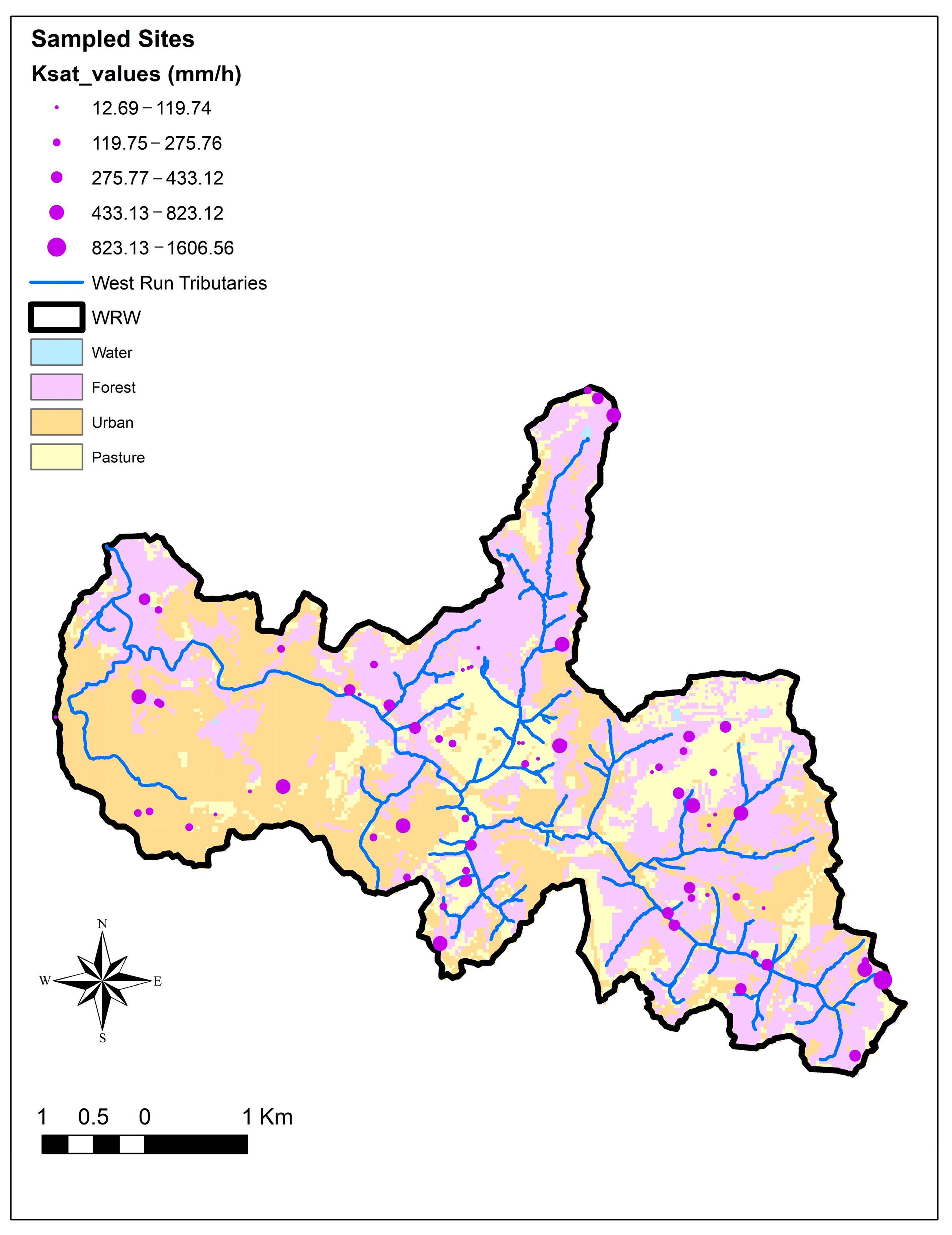
Table 4). The calibration results of the three scenarios showed that the Ksat from all soil layers decreased by 17.21%. The observed saturated hydraulic conductivity generally varied between 13 and 1607 mm/h in the field. The observed Ksat values were collected at soil depths from 0 to 10 cm in the field. Therefore, the calibrated Ksat of the first soil layer (SOL_K1) was replaced with observed Ksat values to implement the research purpose of the experiment, and the primary information about soils in other layers was held constant to maintain conditions. The default saturated hydraulic conductivity values for WRW soil within the SWAT interface for the first layers were 3.276, 32.4, 82.8, and 331.2 mm/h. Furthermore, three scenario calibration results indicated that the Ksat from layer 1 of the soil decreased by 17.21%, with no significant difference between the three scenarios. Thus, the calibrated Ksat values in the first soil layer were 2.71, 26.82, 68.55, and 274.2 mm/h. Notably, the observed average Ksat values for urban (234.6 mm/h) and pasture (190.14 mm/h) land use were found to be underestimated by 16.01% and 30.66% when compared to the calibrated Ksat value of 274.2 mm/h. Conversely, the forest land use observed average Ksat value (419.62 mm/h) was overestimated by 53%.
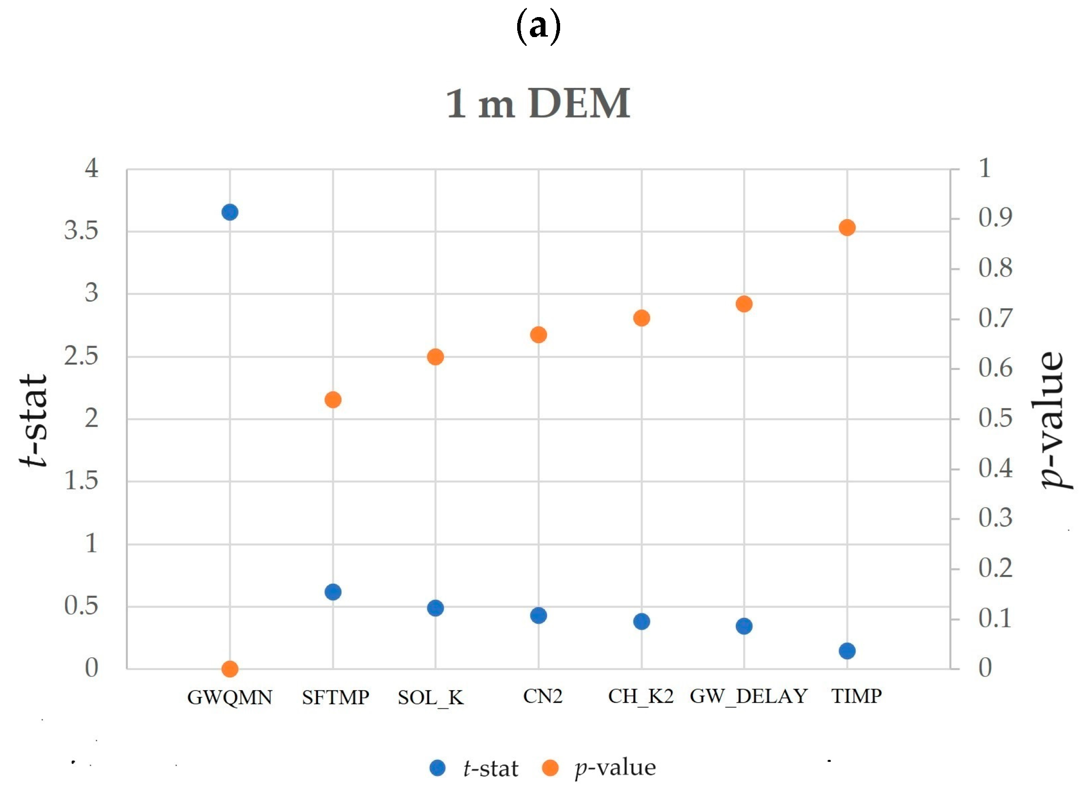
Figure 5 shows the sensitivity analysis results of parameters contributing to the streamflow in the SWAT model of the WRW for the 1 m, 10 m, and 30 m DEMs. Parameters with greater t-stat values and lower p-values were more sensitive, with changes resulting in a higher impact on the streamflow simulations. The shallow aquifer water threshold depth required for return flow (GWQMN) and temperature of snowfall (SFTMP) were the most sensitive parameters for the WRW, as they showed the highest t-stat values and lowest p-values among the seven selected parameters (Figure 5). The comparison between the sensitivity of parameters in different DEM resolutions showed that the 1 m and 30 m DEMs shared the same first three sensitive parameters, while the 10 m DEM only shared two parameters with the 1 m and 30 m DEMs. In the sensitivity analysis of the 1 m DEM, the factors with the highest impact on the streamflow simulation were identified as the shallow aquifer water threshold depth required for return flow (GWQMN), temperature of snowfall (SFTMP), saturated hydraulic conductivity (SOL_K), SCS runoff curve (CN2), effective hydraulic conductivity for the main channel (CH_K2), groundwater delay time (GW_DELAY), and temperature lag snowpack factor (TIMP). In the sensitivity analysis of the 10 m DEM, GWQMN and SFTMP were the top two most sensitive parameters, with CH_K2 as the third, followed by SOL_K, GW_DELAY, CN2, and TIMP. In addition to the top three most sensitive parameters in the 30 m DEM sensitivity analysis, which were the same as those identified in the 1 m DEM analysis, CH_K2, GW_DEALY, CN2, and TIMP were also identified as sensitive parameters in the 30 m DEM analysis, in the same order as in the 10 m DEM analysis, except CH_K2. These results align with the findings of Nazari-Sharabian et al. [55], who showed that specific parameters may become more or less sensitive depending on the resolution threshold above or below.
The calibration and validation performance of the model is presented in Table 5, and Figure 6 compares the three model simulations with observed data using monthly values. The R2 value obtained from the three DEMs during calibration ranged from 0.75 to 0.76, indicating a good correlation between observed and simulated streamflow data. The PBIAS values (−10.6, −11.4, and −12.8) for streamflow simulation in WRW were negative, revealing that 10.6%, 11.4%, and 12.8% of monthly streamflow in the calibration period are overestimated. During the validation period, the R2 values for the three DEMs ranged between 0.72 and 0.73, with higher R2 values indicating less error variance. Based on the three statistical indices (NSE, R2, and PBIAS), the SWAT model performance with the three DEMs is at least satisfactory (R2 > 0.7, NSE > 0.55, and PBIAS ≤ ±15%) [63].
Given that land use and soil types remained unchanged during model simulations, any differences in watershed delineation and streamflow generation were attributed to DEM resolution differences. As anticipated, the resolution of the DEM data impacted the number of subbasins and the layout of streams. For instance, subbasins decreased from 20 to 18 when the DEM resolutions were changed from 1 m to 10 m or 30 m. Similarly, the recommended drainage areas for streams also varied with DEM resolution, being 22.77 km2 for the 1 m DEM, 22.6 km2 for the 10 m DEM, and 21.81 km2 for the 30 m DEM. The 1 m DEM generated a model-delineated area closest to the actual WRW area compared with other DEMs (Table 6). The 1 m DEM also generated more HRUs (122) than the 10 m (86) and 30 m (87) DEMs. Furthermore, the 1 m DEM generated a streamflow of 0.315 m3/s, which was only 7.98% higher than the observed value (0.292 m3/s) at the streamflow monitoring site in the WRW (Figure 1). Therefore, the results generally confirm that the higher-resolution 1 m DEM produced more detailed and accurate SWAT model output than the 10 m and 30 m DEMs.

3.3. Impact of DEM Resolutions on the SWAT Model Output

According to the topographic and watershed characteristics calculated from the respective DEM resolutions, the 1 m DEM scenario showed results closer to the actual watershed conditions than the other two DEM scenarios. Therefore, the 1 m DEM scenario output was a baseline scenario to quantify the SWAT model output uncertainties.
The effect of different DEM scenarios on the SWAT model annual output is shown in Figure 7. Surface runoff, lateral flow, groundwater flow, percolation flow, evapotranspiration (ET), and water yield are the most common interest outputs for water balance components in SWAT model studies [71,72,73,74]. Comparison of the RDs in the modeled outputs indicated that coarser DEM resolutions (10 m and 30 m) affect the model output uncertainties. The overall uncertainty of the annual SWAT model output increased, as the absolute RD values in Figure 7b were higher than the absolute RD values in Figure 7a. The absolute RD values indicated that DEM resolution (10 m and 30 m) had minor impacts on the surface runoff, ET, and water yield, which ranged from 0.89 to 6.75% (less than 15%). Therefore, the effect of DEM resolution was considered negligible. However, the RD values of groundwater flow for the 30 m resolution were from 11.38% up to 23.41%, which were greater RD values than observed for the 10 m DEM scenario. Furthermore, the 30 m DEM resolution also greatly affected the lateral flow, and its absolute RD values were from 17.05% to 17.22%, in a pattern similar to that of the percolation flow.
Uncertainty analysis indicated that the influence of DEM resolutions on surface runoff, ET, and water yield was negligible, as the mean absolute RD values ranged from 0.77% to 3.5%, on average less than 15%. Therefore, the uncertainty analysis for the monthly SWAT model output was focused on lateral flow, groundwater flow, and percolation flow. The effects of the 10 m DEM and 30 m DEM resolution scenarios on these three components at the monthly scale are shown in Figure 8. The overall uncertainty increased as the resolution increased from 1 m to 30 m. The percolation and groundwater flow were overestimated within coarser DEMs (10 m and 30 m) and monthly time series. Specifically, RD values of percolation flow ranged from 1.6% to 21.18% and from 5.34% to 23.59% in the 10 m and 30 m DEM scenarios, respectively. Groundwater flow exhibited a similar pattern, with the most significant RD values being 21.24% and 39.98% in the 10 m and 30 m DEM scenarios, respectively. The mean RD value of groundwater flow in the 30 m DEM resolution scenario was 20.25%, exceeding 15% on average. The absolute RD values for the monthly lateral flow were less than 10%, indicating that the lateral flow changed little with the 10 m DEM resolution impact. Interestingly, the 30 m DEM resolution had a more significant impact on the lateral flow, with most absolute RD values greater than 15%, and these absolute values were nearly twice as large as the absolute RD values in the 10 m DEM resolution scenario.

3.4. Water Balance Components Analysis Based on Observed Ksat

This study’s water balance components (lateral flow, groundwater flow, percolation flow, evapotranspiration, surface runoff, and water yield) were derived from the principles outlined in the SWAT documentation [16]. Figure 9a–c presents the total contributions of the water balance components in the WRW. The results (i.e., lateral flow, groundwater, and percolation flow) of the one-way ANOVA showed that the outputs of the calibrated model (1 m, 10 m, and 30 m) were significantly different from the outputs obtained after substituting the observed Ksat values (p < 0.05). Furthermore, the lateral flow increased the most among these six components after the observed Ksat values were applied to the output of the calibrated model (1 m, 10 m, and 30 m scenarios). Lateral flow using observed Ksat forcings contributed more than lateral flow using the calibrated SWAT model output (478 mm, 447 mm, and 396 mm), ranging from 1113 mm to 1338 mm. Comparatively, groundwater and percolation flow exhibited decreased trends compared to the calibrated model outputs. The groundwater flow and percolation flow ranged from 370 mm to 524 mm and from 628 mm to 851 mm after the observed Ksat values were integrated into the calibrated model’s output (1 m, 10 m, and 30 m scenarios). In addition, water yield increased after observed Ksat values were applied. However, the difference was non-significant based on one-way ANOVA results (p > 0.05). Both evapotranspiration and surface runoff slightly declined after observed Ksat values were used in model simulations. These results are similar to the work of Bauwe et al. [75], who found that the value of Ksat affects the estimation of water balance components. For example, if Ksat is 10 mm/h or smaller, the SWAT model generates more surface runoff [75]. Still, some water balance components exhibited insignificant differences in the model simulation. However, insignificance should not be taken to mean that these changes would not be enough to impose hydrological or aquatic ecological challenges for the WRW.
Lateral flow showed an overall increase after the calibrated Ksat values were substituted by the observed Ksat values in the model simulations, ranging from 635 mm to over 900 mm, depending on the three different DEM scenarios (Table 7). The Ksat-F (forest land use) had the most considerable impact on the lateral flow, contributing to an average increase of 874 mm across the three model outputs, followed by Ksat-U (urban land use) (724 mm) and Ksat-P (pasture land use) (674 mm). This result is presumably due to the specific hydrological characteristics of forest areas, such as the soil with a relatively high infiltration rate due to the native forest vegetation and minimal anthropogenic disturbance [42]. This finding is similar to the research of Neitsch et al. [16], who showed that lateral flow becomes more significant in areas with high-hydraulic-conductivity soil in surface layers at a shallow depth. In contrast, the groundwater and percolation flows decreased after the observed Ksat values were applied in the model simulation. The Ksat-F values caused the most significant reduction in the 30 m DEM scenario, where the groundwater flow declined by 552 mm and the percolation flow declined by 751 mm. The groundwater and percolation flow showed the smallest reduction, 340 mm and 487 mm, under the Ksat-P impact in the 1 m DEM model scenario.
Additionally, the average groundwater flow decrease across the three model outputs was 489 mm for Ksat-F, 420 mm for Ksat-U, and 384 mm for Ksat-P. Similarly, the percolation flow exhibited a higher decrease than the groundwater flow, with an overall average decline of 694 mm for Ksat-F, 561 mm for Ksat-U, and 514 mm for Ksat-P. The percolation flow decline ranged from a minimum of 487 mm to a maximum of 751 mm. These results indicated that different land use types may influence groundwater flow and percolation flow patterns. Astuti et al. [76] and Sertel et al. [77] showed a similar impact of urbanization on percolation flow and groundwater flow. The impervious surface caused by urban expansion decreased infiltration, affecting aquifer recharge and hydrological processes.
The observed Ksat values for forest, pasture, and urban land types caused an overall increase in water yield relative to the calibrated SWAT model output in the three DEM model scenarios, but the average increase was less than the lateral flow. Furthermore, the surface runoff and evapotranspiration showed declining trends after the calibrated Ksat values were replaced with the observed Ksat values in the model simulations. The lowest average changes in the surface runoff were 39 mm with Ksat-F, 36 mm for Ksat-P, and 37 mm for Ksat-U.
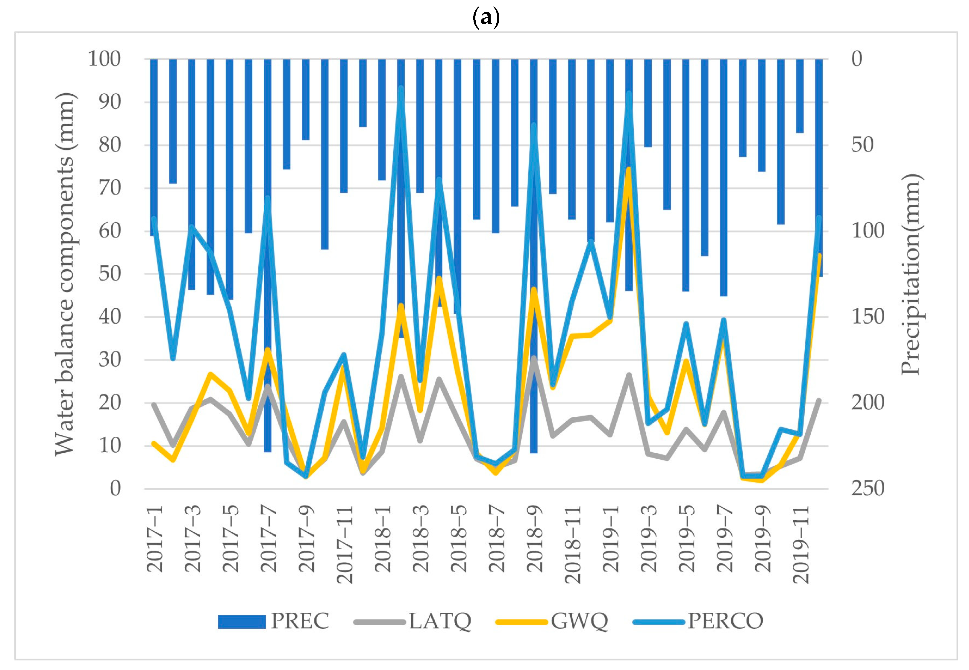
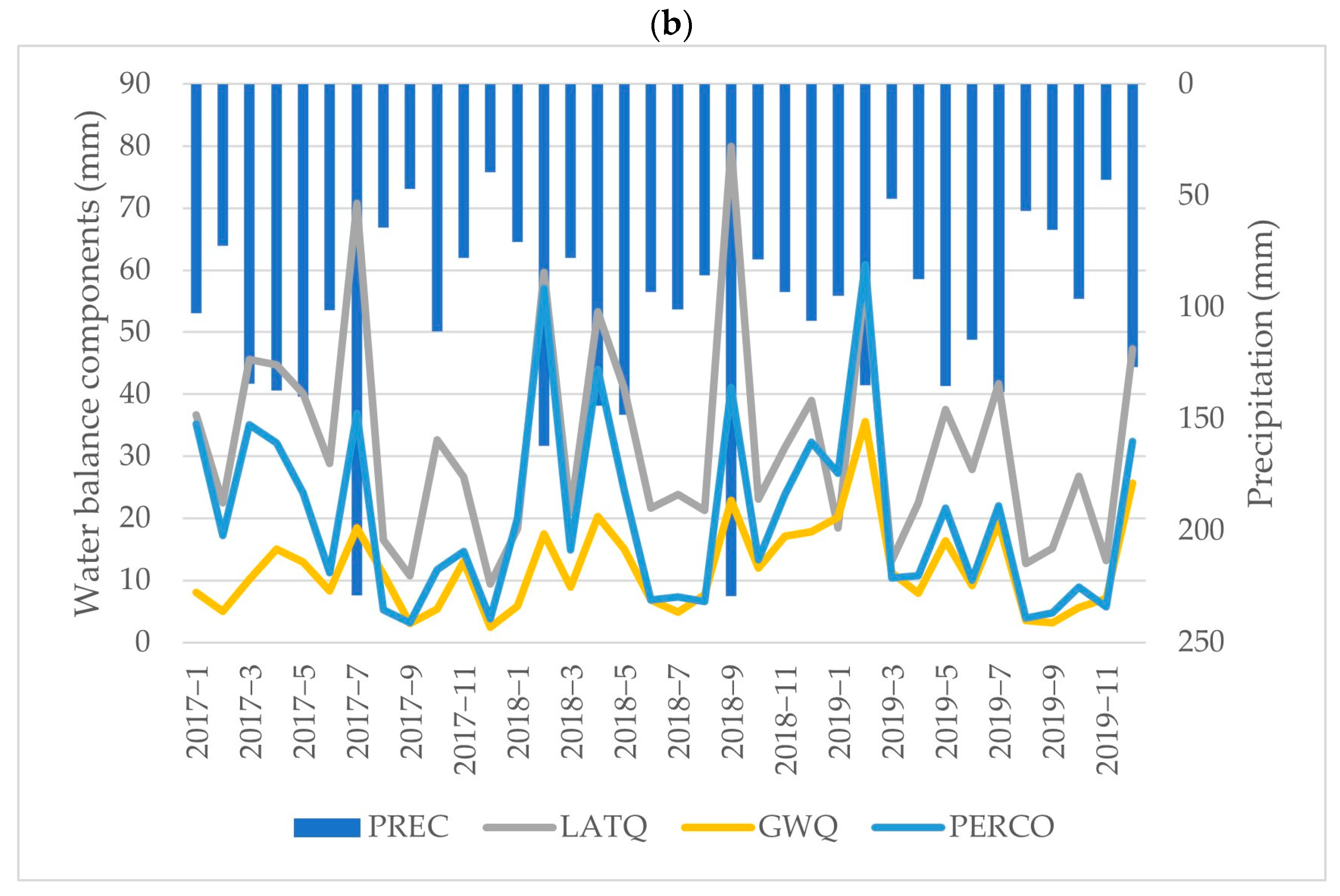
Given the preceding results, scenario 1—Ksat-U (Figure 4) was used as a reference to demonstrate the general impact of observed Ksat on the dynamics of water balance component changes over time in this study. The most significant annual precipitation (PREC) was simulated in 2018, with a total of 1390 mm, a maximum of 229 mm in September, and a minimum of 71 mm in January (Figure 10). Conversely, 2019 had the lowest precipitation among the analyzed years (1144 mm), 112 mm less than the amount generated in 2017 (1256 mm). All variables vary temporally with rainfall patterns (Figure 10a). In scenario 1—Ksat-U, the Ksat value associated with urban land use emerged as a factor driving an increase in lateral flow (LATQ) within the water balance components; however, this increase was at the cost of reduced groundwater (GWQ) and percolation flow. Lateral flow replaced percolation flow in terms of increasing the most when a high precipitation event occurred (Figure 10b). This dynamic interaction between various water balance components emphasizes the relationship between soil properties, hydrological processes, and their combined impact on watershed hydrologic processes.

3.5. Impact of Observed Ksat on the SWAT Output

Figure 11 shows the relative difference (RD) values among the lateral, groundwater, and percolation flows in the 1 m DEM scenario compared to scenario 1—Ksat-U. The observed Ksat greatly impacted these water balance components, with mean absolute RD values exceeding 15% on average. Lateral flow was overestimated after the observed Ksat was incorporated into the model simulation. Groundwater and percolation flow exhibited a similar trend; the mean RD values were −33.01% and −32.36%, respectively. The RD values of groundwater flow and percolation flow fluctuated slightly over time. Both parameters tended to be overestimated around summertime. However, most RD values remained below 0, indicating that groundwater and percolation flow were predominantly underestimated under scenario 1—Ksat-U.

4. Discussion

This research resulted in an exploratory modeling approach in the SWAT model framework to investigate the SWAT model simulation response to field-measured Ksat values under three DEM resolutions. Figure 7 shows that DEM resolution impacted model predictive outputs. The overall uncertainty of model outputs increased as the DEM resolution became coarser, evidenced by the absolute RD values (>15%). A minor impact was found on surface runoff, water yield, and ET, consistent with previous research [32,33,46,64,65]. For example, the results of Song et al. [33] showed that the simulated values of surface runoff change gently, and this value dropped by 2% when DEM resolution increased from 10 m to 130 m. Lin et al. [32] used the DEM resolution from 5 m to 140 m, and they also found similar results, namely that the relative difference (RD) of simulated runoff was less than 1%. Di Luzio et al. [78] explained that surface runoff was computed using the SCS curve number method, and DEM resolution did not affect the average curve number value. Sukumaran and Sahoo [64] pointed out that since surface runoff constituted a significant portion of water yield, variations in water yield were predominantly reflected by changes in surface runoff. Given the insensitivity of surface runoff to DEM resolutions, water yield was also not sensitive to the DEM resolutions. Further uncertainty analysis revealed that the 30 m DEM resolution had a more significant influence on the lateral flow, groundwater, and percolation flow than the 10 m DEM resolution. The groundwater flow (mean RDannual = 19.32% and mean RDmonthly = 20.25%) and percolation flow (mean RDannual = 9.43% and mean RDmonthly = 12.86%) tended to be overestimated, and the lateral flow (mean RDannual = −17.13% and mean RDmonthly = −17.09%) tended to be underestimated on both annual and monthly scales.
Mean observed Ksat values were forced in the calibrated SWAT model with different DEM resolutions to generate distinct DEM scenarios. One-way analysis of variance (ANOVA) indicated that the mean observed Ksat had a significant (p < 0.05) impact on the lateral flow, groundwater flow, and percolation flow (outputs) of the SWAT model within three DEM resolution scenarios. Furthermore, the uncertainty in SWAT model output within these DEM scenarios was changed relative to DEM resolution, and extra Ksat data were incorporated into the model simulation. Figure 11 shows the impact of the mean observed Ksat (urban land use) on model output and isolates the disturbed DEM resolution effect. The mean observed Ksat (urban land use) changed the SWAT model output uncertainty under the 1 m DEM scenario. The monthly lateral flow was overestimated, with mean RD values of 164.98%. Conversely, the overall RD values of monthly groundwater and percolation flow were negative, indicating that they were underestimated. However, both tended to be overestimated (RD values ranged from 7.01% to 63.21%) in the summer months.

5. Study Limitations and Future Directions

This study is among the first to test the impact of observed Ksat values on water balance components, incorporating the influence of DEM resolution. Despite its notable contributions, the study contains certain limitations. The field Ksat data collection did not include subsurface soil Ksat values. Ksat may vary with soil depth, and this omission could potentially affect model predictions, as more observed data might enhance the model performance and reduce model simulation uncertainty [20,25,31,69,79]. In addition, this study showed that 1 m DEM could provide a more detailed and accurate analysis in this study relative to coarser DEMs. However, 1 m DEMs may be impractical for a large catchment. Finally, while the time series duration was adequate for the current investigation, the relatively short period of available streamflow may affect model simulation accuracy. The more extended streamflow dataset includes several wet- and dry-year records, which may increase the reliability of the model calibration. In future research, investigators may wish to include additional field observations (i.e., observed field Ksat data with multiple soil depths) to validate and characterize interactions between observed Ksat and the estimation of water balance components while considering the impact of DEM resolution. Despite these limitations, the current study offers valuable insights into the nuanced relationship between Ksat and water balance components relative to DEM resolution, enriching the SWAT model research literature and contributing to improving hydrological modeling predictions. Also, investigators could consider the estimation of a single water balance component (e.g., evapotranspiration from weather data) to constrain the model further. While beyond the scope of the current study, this approach may provide impetus for future work.

6. Conclusions

This investigation used an exploratory modeling approach to assess observed Ksat values on water balance components under three DEM resolutions in a representative Appalachian mixed-land-use watershed. The model’s performance was assessed using statistical indicators (NSE, R2, and PBIAS), and three DEMs showed satisfactory (or better) performance in both calibration (R2 > 0.74, NSE > 0.72, and PBIAS ≤ ±13%) and validation (R2 > 0.71, NSE > 0.70, and PBIAS ≤ ±6%) periods. The sensitivity analysis from SWAT-CUP indicated that the most sensitive calibration parameters were the shallow aquifer water threshold depth for return flow (GWQMN) and the temperature of snowfall (SFTMP), which is essential for snowmelt threshold estimations and thus soil water infiltration processes. This observation was consistent across all three DEM scenarios. The novelty of this work includes the developed exploratory modeling method that could incorporate observed field Ksat value into the model simulation with the help of SWAT-related software (SWAT-CUP, version: 2012) under different DEM resolution scenarios. In addition, this work also quantifies the uncertainty in the model output caused by observed field Ksat and DEM resolution scenarios. It is worth noting that this methodology includes the flexibility to adapt to differences in model output attributed to differences between observed field Ksat model forcings or DEM resolutions. The uncertainty analysis indicated that observed Ksat and DEM resolutions inevitably affect the model output, especially the lateral flow, percolation flow, and groundwater flow (RD > 15%), and the observed Ksat had a more significant impact on model output than DEM resolutions. These findings offer quantitative evidence on model output, providing valuable insights for hydrologists and modelers to understand how observed Ksat affects model output relative to empirically derived Ksat under multiple DEM resolution scenarios.

Author Contributions

Conceptualization, J.A.H. and J.A.T.; methodology, J.A.H., L.J., S.J.H. and J.A.T.; software, J.A.H.; validation, J.A.H. and L.J.; formal analysis, J.A.H. and L.J.; investigation, L.J. and J.A.H.; resources, J.A.H.; data curation, L.J., J.A.T., S.J.H. and J.A.H.; writing—original draft preparation, L.J. and J.A.H.; writing—review and editing, L.J., J.A.H., S.J.H., J.A.T., S.E.C. and M.P.S.; visualization, J.A.H. and L.J.; supervision, J.A.H.; project administration, J.A.H.; funding acquisition, J.A.T. and J.A.H. All authors have read and agreed to the published version of the manuscript.

Funding

This work was supported by the USDA National Institute of Food and Agriculture, Hatch project accession number 1011536 and McIntire Stennis accession number 7003934, and the West Virginia Agricultural and Forestry Experiment Station. Additional funding was provided by the USDA Natural Resources Conservation Service, Soil and Water Conservation, Environmental Quality Incentives Program No. 68-3D47-18-005, and a portion of this research was supported by the Agriculture and Food Research Initiative Competitive Grant No. 2020-68012-31881 from the USDA National Institute of Food and Agriculture. The results presented may not reflect the sponsors’ views, and no official endorsement should be inferred. The funders had no role in study design, data collection and analysis, the decision to publish, or the preparation of the manuscript.

Data Availability Statement

The data presented in this study are available on request from the corresponding author. The data are not publicly available due to proprietary concerns. Other data are available through publicly available sources noted in text.

Acknowledgments

The authors appreciate the feedback of anonymous reviewers whose constructive comments improved the article.

Conflicts of Interest

The authors declare no conflicts of interest.

References

  1. Wu, L.; Pan, L.; Mitchell, J.; Sanden, B. Measuring Saturated Hydraulic Conductivity Using a Generalized Solution for Single-Ring Infiltrometers. Soil Sci. Soc. Am. J. 1999, 63, 788–792. [Google Scholar] [CrossRef]
  2. Hwang, H.-T.; Jeen, S.-W.; Suleiman, A.; Lee, K.-K. Comparison of Saturated Hydraulic Conductivity Estimated by Three Different Methods. Water 2017, 9, 942. [Google Scholar] [CrossRef]
  3. Jabro, J.D. Estimation of Saturated Hydraulic Conductivity of Soils from Particle Size Distribution and Bulk Density Data. Trans. ASAE 1992, 35, 557–560. [Google Scholar] [CrossRef]
  4. Zhang, S.Y.; Hopkins, I.; Guo, L.; Lin, H. Dynamics of Infiltration Rate and Field-Saturated Soil Hydraulic Conductivity in a Wastewater-Irrigated Cropland. Water 2019, 11, 1632. [Google Scholar] [CrossRef]
  5. Zhang, Y.; Schaap, M.G. Estimation of Saturated Hydraulic Conductivity with Pedotransfer Functions: A Review. J. Hydrol. 2019, 575, 1011–1030. [Google Scholar] [CrossRef]
  6. Sahoo, G.B.; Ray, C.; De Carlo, E.H. Calibration and Validation of a Physically Distributed Hydrological Model, MIKE SHE, to Predict Streamflow at High Frequency in a Flashy Mountainous Hawaii Stream. J. Hydrol. 2006, 327, 94–109. [Google Scholar] [CrossRef]
  7. Black, J.H. The Practical Reasons Why Slug Tests (Including Falling and Rising Head Tests) Often Yield the Wrong Value of Hydraulic Conductivity. Q. J. Eng. Geol. Hydrogeol. 2010, 43, 345–358. [Google Scholar] [CrossRef]
  8. Duan, R.; Fedler, C.B.; Borrelli, J. Comparison of Methods to Estimate Saturated Hydraulic Conductivity in Texas Soils with Grass. J. Irrig. Drain. Eng. 2012, 138, 322–327. [Google Scholar] [CrossRef]
  9. Sihag, P.; Esmaeilbeiki, F.; Singh, B.; Ebtehaj, I.; Bonakdari, H. Modeling Unsaturated Hydraulic Conductivity by Hybrid Soft Computing Techniques. Soft Comput. 2019, 23, 12897–12910. [Google Scholar] [CrossRef]
  10. Thomas, S.K.; Conta, J.F.; Severson, E.D.; Galbraith, J.M. Measuring Saturated Hydraulic Conductivity in Soil (No. CSES-141P); Virginia Cooperative Extension: Stafford, VA, USA, 2016; pp. 1–13. [Google Scholar]
  11. Gootman, K.; Kellner, E.; Hubbart, J. A Comparison and Validation of Saturated Hydraulic Conductivity Models. Water 2020, 12, 2040. [Google Scholar] [CrossRef]
  12. Bagarello, V.; Iovino, M.; Tusa, G. Factors Affecting Measurement of the Near-Saturated Soil Hydraulic Conductivity. Soil Sci. Soc. Am. J. 2000, 64, 1203–1210. [Google Scholar] [CrossRef]
  13. Dai, Y.; Shangguan, W.; Duan, Q.; Liu, B.; Fu, S.; Niu, G. Development of a China Dataset of Soil Hydraulic Parameters Using Pedotransfer Functions for Land Surface Modeling. J. Hydrometeorol. 2013, 14, 869–887. [Google Scholar] [CrossRef]
  14. Elbisy, M.S. Support Vector Machine and Regression Analysis to Predict the Field Hydraulic Conductivity of Sandy Soil. KSCE J. Civ. Eng. 2015, 19, 2307–2316. [Google Scholar] [CrossRef]
  15. Hvorslev, M.J. Time Lag and Soil Permeability in Ground-Water Observations. US Army Corps Eng. Waterw. Exp. Stn. Bull 1951, 36, 1–50. [Google Scholar]
  16. Neitsch, S.L.; Arnold, J.G.; Kiniry, J.R.; Williams, J.R. Soil and Water Assessment Tool Theoretical Documentation Version 2009; Texas Water Resources Institute, 2011. Available online: https://swat.tamu.edu/media/99192/swat2009-theory.pdf (accessed on 10 March 2023).
  17. Reynolds, W.D.; Bowman, B.T.; Brunke, R.R.; Drury, C.F.; Tan, C.S. Comparison of Tension Infiltrometer, Pressure Infiltrometer, and Soil Core Estimates of Saturated Hydraulic Conductivity. Soil Sci. Soc. Am. J. 2000, 64, 478–484. [Google Scholar] [CrossRef]
  18. Vereecken, H.; Weynants, M.; Javaux, M.; Pachepsky, Y.; Schaap, M.G.; van Genuchten, M.T. Using Pedotransfer Functions to Estimate the van Genuchten-Mualem Soil Hydraulic Properties: A Review. Vadose Zone J. 2010, 9, 795–820. [Google Scholar] [CrossRef]
  19. Vienken, T.; Dietrich, P. Field Evaluation of Methods for Determining Hydraulic Conductivity from Grain Size Data. J. Hydrol. 2011, 400, 58–71. [Google Scholar] [CrossRef]
  20. Abesh, B.F.; Hubbart, J.A. A Comparison of Saturated Hydraulic Conductivity (Ksat) Estimations from Pedotransfer Functions (PTFs) and Field Observations in Riparian Seasonal Wetlands. Water 2023, 15, 2711. [Google Scholar] [CrossRef]
  21. Kannan, N.; White, S.M.; Worrall, F.; Whelan, M.J. Sensitivity Analysis and Identification of the Best Evapotranspiration and Runoff Options for Hydrological Modelling in SWAT-2000. J. Hydrol. 2007, 332, 456–466. [Google Scholar] [CrossRef]
  22. Busico, G.; Colombani, N.; Fronzi, D.; Pellegrini, M.; Tazioli, A.; Mastrocicco, M. Evaluating SWAT Model Performance, Considering Different Soils Data Input, to Quantify Actual and Future Runoff Susceptibility in a Highly Urbanized Basin. J. Environ. Manag. 2020, 266, 110625. [Google Scholar] [CrossRef] [PubMed]
  23. Ntona, M.M.; Busico, G.; Mastrocicco, M.; Kazakis, N. Coupling SWAT and DPSIR Models for Groundwater Management in Mediterranean Catchments. J. Environ. Manag. 2023, 344, 118543. [Google Scholar] [CrossRef]
  24. Thompson, J.A.; Bell, J.C.; Zanner, C.W. Hydrology and Hydric Soil Extent within a Mollisol Catena in Southeastern Minnesota. Soil Sci. Soc. Am. J. 1998, 62, 1126–1133. [Google Scholar] [CrossRef]
  25. Arnold, J.G.; Moriasi, D.N.; Gassman, P.W.; Abbaspour, K.C.; White, M.J.; Srinivasan, R.; Santhi, C.; Harmel, R.D.; van Griensven, A.; van Liew, M.W.; et al. SWAT: Model Use, Calibration, and Validation. Trans. ASABE 2012, 55, 1491–1508. [Google Scholar] [CrossRef]
  26. Gassman, P.W.; Reyes, M.R.; Green, C.H.; Arnold, J.G. The Soil and Water Assessment Tool: Historical Development, Applications, and Future Research Directions. Trans. ASABE 2007, 50, 1211–1250. [Google Scholar] [CrossRef]
  27. Tan, M.L.; Gassman, P.W.; Yang, X.; Haywood, J. A Review of SWAT Applications, Performance and Future Needs for Simulation of Hydro-Climatic Extremes. Adv. Water Resour. 2020, 143, 103662. [Google Scholar] [CrossRef]
  28. Abbaspour, K.C. SWAT-CUP: SWAT Calibration and Uncertainty Programs—A User Manual; Eawag: Dübendorf, Switzerland, 2015; pp. 17–66. [Google Scholar]
  29. Spruill, C.A.; Workman, S.R.; Taraba, J.L. Simulation of daily and monthly stream discharge from small watersheds using the swat model. Trans. ASAE 2000, 43, 1431–1439. [Google Scholar] [CrossRef]
  30. Huisman, J.A.; Breuer, L.; Frede, H.-G. Sensitivity of Simulated Hydrological Fluxes towards Changes in Soil Properties in Response to Land Use Change. Phys. Chem. Earth Parts ABC 2004, 29, 749–758. [Google Scholar] [CrossRef]
  31. Rocha, J.; Duarte, A.; Fabres, S.; Quintela, A.; Serpa, D. Influence of DEM Resolution on the Hydrological Responses of a Terraced Catchment: An Exploratory Modelling Approach. Remote Sens. 2022, 15, 169. [Google Scholar] [CrossRef]
  32. Lin, S.; Jing, C.; Coles, N.A.; Chaplot, V.; Moore, N.J.; Wu, J. Evaluating DEM Source and Resolution Uncertainties in the Soil and Water Assessment Tool. Stoch. Environ. Res. Risk Assess. 2013, 27, 209–221. [Google Scholar] [CrossRef]
  33. Song, X.; Qi, Z.; Du, L.P.; Kou, C.L. The Influence of DEM Resolution on Hydrological Simulation in the Huangshui River Basin. Adv. Mater. Res. 2012, 518–523, 4299–4302. [Google Scholar] [CrossRef]
  34. Petersen, F.; Hubbart, J.A.; Kellner, E.; Kutta, E. Land-Use-Mediated Escherichia Coli Concentrations in a Contemporary Appalachian Watershed. Environ. Earth Sci. 2018, 77, 754. [Google Scholar] [CrossRef]
  35. Horne, J.P.; Hubbart, J.A. A Spatially Distributed Investigation of Stream Water Temperature in a Contemporary Mixed-Land-Use Watershed. Water 2020, 12, 1756. [Google Scholar] [CrossRef]
  36. Kellner, E.; Hubbart, J.; Stephan, K.; Morrissey, E.; Freedman, Z.; Kutta, E.; Kelly, C. Characterization of Sub-Watershed-Scale Stream Chemistry Regimes in an Appalachian Mixed-Land-Use Watershed. Environ. Monit. Assess. 2018, 190, 586. [Google Scholar] [CrossRef] [PubMed]
  37. Kutta, E.; Hubbart, J. Climatic Trends of West Virginia: A Representative Appalachian Microcosm. Water 2019, 11, 1117. [Google Scholar] [CrossRef]
  38. Abesh, B.F.; Jin, L.; Hubbart, J.A. Predicting Climate Change Impacts on Water Balance Components of a Mountainous Watershed in the Northeastern USA. Water 2022, 14, 3349. [Google Scholar] [CrossRef]
  39. Hubbart, J.A.; Kellner, E.; Petersen, F. A 22-Site Comparison of Land-Use Practices, E-Coli and Enterococci Concentrations. Int. J. Environ. Res. Public Health 2022, 19, 13907. [Google Scholar] [CrossRef] [PubMed]
  40. Heck, Z.A. Development of Multi-Catchment Rating Curves for Streams of Appalachian Mixed-Land-Use Watersheds: Preliminary Results; West Virginia University Libraries: Morgantown, WV, USA, 2021. [Google Scholar]
  41. Malone, B.P.; Minansy, B.; Brungard, C. Some Methods to Improve the Utility of Conditioned Latin Hypercube Sampling. PeerJ 2019, 7, e6451. [Google Scholar] [CrossRef] [PubMed]
  42. Higgins, S.J. Mapping Infiltration in an Urbanizing Mixed-Land-Use Watershed with Multi-Temporal Satellite Imagery; West Virginia University Libraries: Morgantown, WV, USA, 2023. [Google Scholar]
  43. Dessu, S.B.; Melesse, A.M. Modelling the Rainfall-Runoff Process of the Mara River Basin Using the Soil and Water Assessment Tool: Mara river basin: Rainfall-runoff process. Hydrol. Process. 2012, 26, 4038–4049. [Google Scholar] [CrossRef]
  44. Cao, W.; Bowden, W.B.; Davie, T.; Fenemor, A. Multi-Variable and Multi-Site Calibration and Validation of SWAT in a Large Mountainous Catchment with High Spatial Variability. Hydrol. Process. 2006, 20, 1057–1073. [Google Scholar] [CrossRef]
  45. Singh, L.; Saravanan, S. Simulation of Monthly Streamflow Using the SWAT Model of the Ib River Watershed, India. HydroResearch 2020, 3, 95–105. [Google Scholar] [CrossRef]
  46. Tan, M.L.; Ramli, H.P.; Tam, T.H. Effect of DEM Resolution, Source, Resampling Technique and Area Threshold on SWAT Outputs. Water Resour. Manag. 2018, 32, 4591–4606. [Google Scholar] [CrossRef]
  47. Rouholahnejad, E.; Abbaspour, K.C.; Srinivasan, R.; Bacu, V.; Lehmann, A. Water Resources of the Black Sea Basin at High Spatial and Temporal Resolution. Water Resour. Res. 2014, 50, 5866–5885. [Google Scholar] [CrossRef]
  48. Cerro, I.; Antigüedad, I.; Srinavasan, R.; Sauvage, S.; Volk, M.; Sanchez-Perez, J.M. Simulating Land Management Options to Reduce Nitrate Pollution in an Agricultural Watershed Dominated by an Alluvial Aquifer. J. Environ. Qual. 2014, 43, 67–74. [Google Scholar] [CrossRef] [PubMed]
  49. Mishra, A.; Kar, S. Modeling Hydrologic Processes and NPS Pollution in a Small Watershed in Subhumid Subtropics Using SWAT. J. Hydrol. Eng. 2012, 17, 445–454. [Google Scholar] [CrossRef]
  50. Sun, W.; Wang, Y.; Wang, G.; Cui, X.; Yu, J.; Zuo, D.; Xu, Z. Physically Based Distributed Hydrological Model Calibration Based on a Short Period of Streamflow Data: Case Studies in Four Chinese Basins. Hydrol. Earth Syst. Sci. 2017, 21, 251–265. [Google Scholar] [CrossRef]
  51. Li, Z.; Jian, S.; Gu, R.; Sun, J. Runoff Simulation under the Effects of the Modified Soil Water Assessment Tool (SWAT) Model in the Jiyun River Basin. Water 2023, 15, 2110. [Google Scholar] [CrossRef]
  52. Abbaspour, K.C.; Yang, J.; Maximov, I.; Siber, R.; Bogner, K.; Mieleitner, J.; Zobrist, J.; Srinivasan, R. Modelling Hydrology and Water Quality in the Pre-Alpine/Alpine Thur Watershed Using SWAT. J. Hydrol. 2007, 333, 413–430. [Google Scholar] [CrossRef]
  53. Abbaspour, K.C.; Johnson, C.A. Estimating Uncertain Flow and Transport Parameters Using a Sequential Uncertainty Fitting Procedure. Vadose Zone J. 2004, 3, 1340–1352. [Google Scholar] [CrossRef]
  54. Malik, M.A.; Dar, A.Q.; Jain, M.K. Modelling Streamflow Using the SWAT Model and Multi-site Calibration Utilizing SUFI-2 of SWAT-CUP Model for High Altitude Catchments, NW Himalaya’s. Model. Earth Syst. Environ. 2022, 8, 1203–1213. [Google Scholar] [CrossRef]
  55. Nazari-Sharabian, M.; Taheriyoun, M.; Karakouzian, M. Sensitivity Analysis of the DEM Resolution and Effective Parameters of Runoff Yield in the SWAT Model: A Case Study. J. Water Supply Res. Technol.-Aqua 2020, 69, 39–54. [Google Scholar] [CrossRef]
  56. Wu, L.; Liu, X.; Yang, Z.; Yu, Y.; Ma, X. Effects of Single- and Multi-Site Calibration Strategies on Hydrological Model Performance and Parameter Sensitivity of Large-Scale Semi-Arid and Semi-Humid Watersheds. Hydrol. Process. 2022, 36, e14616. [Google Scholar] [CrossRef]
  57. van Griensven, A.; Meixner, T.; Grunwald, S.; Bishop, T.; Diluzio, M.; Srinivasan, R. A Global Sensitivity Analysis Tool for the Parameters of Multi-Variable Catchment Models. J. Hydrol. 2006, 324, 10–23. [Google Scholar] [CrossRef]
  58. Paul, M.; Rajib, M.A.; Ahiablame, L. Spatial and Temporal Evaluation of Hydrological Response to Climate and Land Use Change in Three South Dakota Watersheds. JAWRA J. Am. Water Resour. Assoc. 2017, 53, 69–88. [Google Scholar] [CrossRef]
  59. Mehan, S.; Neupane, R.P.; Kumar, S. Coupling of SUFI 2 and SWAT for Improving the Simulation of Streamflow in an Agricultural Watershed of South Dakota. Hydrol. Curr. Res. 2017, 8. [Google Scholar] [CrossRef]
  60. Gupta, H.V.; Kling, H.; Yilmaz, K.K.; Martinez, G.F. Decomposition of the Mean Squared Error and NSE Performance Criteria: Implications for Improving Hydrological Modelling. J. Hydrol. 2009, 377, 80–91. [Google Scholar] [CrossRef]
  61. Nash, J.E.; Sutcliffe, J.V. River Flow Forecasting through Conceptual Models Part I—A Discussion of Principles. J. Hydrol. 1970, 10, 282–290. [Google Scholar] [CrossRef]
  62. Moriasi, D.N.; Arnold, J.G.; Van Liew, M.W.; Bingner, R.L.; Harmel, R.D.; Veith, T.L. Model Evaluation Guidelines for Systematic Quantification of Accuracy in Watershed Simulations. Trans. ASABE 2007, 50, 885–900. [Google Scholar] [CrossRef]
  63. Moriasi, D.N.; Gitau, M.W.; Pai, N.; Daggupati, P. Hydrologic and Water Quality Models: Performance Measures and Evaluation Criteria. Trans. ASABE 2015, 58, 1763–1785. [Google Scholar] [CrossRef]
  64. Sukumaran, H.; Sahoo, S.N. A Methodological Framework for Identification of Baseline Scenario and Assessing the Impact of DEM Scenarios on SWAT Model Outputs. Water Resour. Manag. 2020, 34, 4795–4814. [Google Scholar] [CrossRef]
  65. Zhang, P.; Liu, R.; Bao, Y.; Wang, J.; Yu, W.; Shen, Z. Uncertainty of SWAT Model at Different DEM Resolutions in a Large Mountainous Watershed. Water Res. 2014, 53, 132–144. [Google Scholar] [CrossRef]
  66. Casper, A.F.; Dixon, B.; Earls, J.; Gore, J.A. Linking a Spatially Explicit Watershed Model (SWAT) with an In-stream Fish Habitat Model (PHABSIM): A Case Study of Setting Minimum Flows and Levels in a Low Gradient, Sub-tropical River. River Res. Appl. 2011, 27, 269–282. [Google Scholar] [CrossRef]
  67. Sun, D.; Yang, H.; Guan, D.; Yang, M.; Wu, J.; Yuan, F.; Jin, C.; Wang, A.; Zhang, Y. The Effects of Land Use Change on Soil Infiltration Capacity in China: A Meta-Analysis. Sci. Total Environ. 2018, 626, 1394–1401. [Google Scholar] [CrossRef]
  68. Ali, Q.S.W.; Pandey, S.; Chaudhuri, R.R.; Behera, S.; Jeyakumar, L. Development of Rainfall-Infiltration Measurement System and Recharge Strategies for Urban Flooding Areas: A Case Study of Delhi, India. Model. Earth Syst. Environ. 2021, 7, 2719–2731. [Google Scholar] [CrossRef]
  69. Kurnianto, S.; Selker, J.; Boone Kauffman, J.; Murdiyarso, D.; Peterson, J.T. The Influence of Land-Cover Changes on the Variability of Saturated Hydraulic Conductivity in Tropical Peatlands. Mitig. Adapt. Strateg. Glob. Chang. 2019, 24, 535–555. [Google Scholar] [CrossRef]
  70. Zhou, X.; Lin, H.S.; White, E.A. Surface Soil Hydraulic Properties in Four Soil Series under Different Land Uses and Their Temporal Changes. Catena 2008, 73, 180–188. [Google Scholar] [CrossRef]
  71. Dhami, B.; Himanshu, S.K.; Pandey, A.; Gautam, A.K. Evaluation of the SWAT Model for Water Balance Study of a Mountainous Snowfed River Basin of Nepal. Environ. Earth Sci. 2018, 77, 21. [Google Scholar] [CrossRef]
  72. Garna, R.K.; Fuka, D.R.; Faulkner, J.W.; Collick, A.S.; Easton, Z.M. Watershed Model Parameter Estimation in Low Data Environments. J. Hydrol. Reg. Stud. 2023, 45, 101306. [Google Scholar] [CrossRef]
  73. Leng, M.; Yu, Y.; Wang, S.; Zhang, Z. Simulating the Hydrological Processes of a Meso-Scale Watershed on the Loess Plateau, China. Water 2020, 12, 878. [Google Scholar] [CrossRef]
  74. Tumsa, B.C.; Kenea, G.; Tola, B. The Application of SWAT+ Model to Quantify the Impacts of Sensitive LULC Changes on Water Balance in Guder Catchment, Oromia, Ethiopia. Heliyon 2022, 8, e12569. [Google Scholar] [CrossRef]
  75. Bauwe, A.; Tiedemann, S.; Kahle, P.; Lennartz, B. Does the Temporal Resolution of Precipitation Input Influence the Simulated Hydrological Components Employing the SWAT Model? JAWRA J. Am. Water Resour. Assoc. 2017, 53, 997–1007. [Google Scholar] [CrossRef]
  76. Astuti, I.S.; Sahoo, K.; Milewski, A.; Mishra, D.R. Impact of Land Use Land Cover (LULC) Change on Surface Runoff in an Increasingly Urbanized Tropical Watershed. Water Resour. Manag. 2019, 33, 4087–4103. [Google Scholar] [CrossRef]
  77. Sertel, E.; Imamoglu, M.Z.; Cuceloglu, G.; Erturk, A. Impacts of Land Cover/Use Changes on Hydrological Processes in a Rapidly Urbanizing Mid-Latitude Water Supply Catchment. Water 2019, 11, 1075. [Google Scholar] [CrossRef]
  78. Di Luzio, M.; Arnold, J.G.; Srinivasan, R. Effect of GIS Data Quality on Small Watershed Stream Flow and Sediment Simulations. Hydrol. Process. 2005, 19, 629–650. [Google Scholar] [CrossRef]
  79. Muma, M.; Rousseau, A.; Gumiere, S. Assessment of the Impact of Subsurface Agricultural Drainage on Soil Water Storage and Flows of a Small Watershed. Water 2016, 8, 326. [Google Scholar] [CrossRef]
Figure 1. The West Run Watershed (WRW) located in northern West Virginia (WV), USA (red area, top right).
Water 16 00735 g001
Figure 2. Sampling sites and associated Ksat values (mm/h) in the West Run Watershed (WRW), West Virginia (WV), USA.
Water 16 00735 g002
Figure 3. The methodological framework for calibrating the SWAT hydrological model in the current investigation.
Water 16 00735 g003
Figure 4. Flowchart of the replacement procedure within the SWAT-CUP for the current investigation (WRW), Morgantown, West Virginia, USA. Note: the current figure begins where the previous Figure 3 leaves off.
Water 16 00735 g004
Figure 5. Sensitivity of parameters contributing to the streamflow in the SWAT model using (a) the 1 m DEM, (b) the 10 m DEM, and (c) the 30 m DEM. The definition of these parameters can be found in Table 4 above.
Water 16 00735 g005aWater 16 00735 g005b
Figure 6. SWAT streamflow simulation for the 1 m DEM, 10 m DEM, and 30 m DEM for calibration and validation periods for West Run Watershed, Morgantown, West Virginia, USA.
Water 16 00735 g006
Figure 7. The comparison (relative difference) of annual surface runoff, lateral flow, groundwater flow, percolation flow, evapotranspiration, and water yield (model outputs) for DEM resolutions (10 m and 30 m) with the 1 m DEM, (a) 10 m DEM compared with 1 m DEM, (b) 30 m DEM compared with 1 m DEM.
Water 16 00735 g007
Figure 8. The comparison (relative difference) of the monthly lateral flow, groundwater flow, and percolation flow (model outputs) for DEM resolutions (10 m and 30 m) with the 1 m DEM, (a) 10 m DEM compared with 1 m DEM, (b) 30 m DEM compared with 1 m DEM.
Water 16 00735 g008aWater 16 00735 g008b
Figure 9. Total contributions of hydrological components to the water balance for the WRW: (a) 1 m DEM water balance components, (b) 10 m DEM water balance components, (c) 30 m DEM water balance components (mm).
Water 16 00735 g009
Figure 10. Time series of various simulated components: (a) 1 m DEM calibrated output, (b) scenario 1—Ksat-U output.
Water 16 00735 g010aWater 16 00735 g010b
Figure 11. The comparison (relative difference) of various simulated components in the 1 m DEM calibrated output with scenario 1—Ksat-U output over time.
Water 16 00735 g011
Table 1. Data types, descriptions, and sources of map units used in the SWAT model in the current study.
Data TypesDescriptionsData SourcesResolution/Scale/Year
DEM-1Digital elevation modelWVU GIS Technical Center http://data.wvgis.wvu.edu/elevation/ (accessed on 15 April 2023)1 m
DEM-10Digital elevation modelUSGS National Map https://apps.nationalmap.gov/downloader/ (accessed on 15 April 2023)10 m
DEM-30Digital elevation modelUSGS National Map https://apps.nationalmap.gov/downloader/ (accessed on 15 April 2023)30 m
Land UseWV land use land cover WVU GIS Technical Center https://wvgis.wvu.edu/data/dataset.php?ID=489 (accessed on 13 April 2023)5 m
SoilSoil Survey Geographic Database (SSURGO) Natural Resources Conservation Service (NRCS) https://www.nrcs.usda.gov/resources/data-and-reports/soil-survey-geographic-database-ssurgo (accessed on 20 April 2023)1:24,000
Meteorological DataDaily precipitation data and temperature dataNational Climate Data Center (NCDC) USW00013736 Morgantown Municipal Airport https://www.ncei.noaa.gov/ (accessed on 21 April 2023)2001–2021
Table 2. Description of the initial calibration parameters for West Run Watershed, Morgantown, West Virginia, USA.
Parameter IdentifierParameterDetailed Parameter Description
RCN2.mgtSCS curve number for moisture condition II
RSOL_K.solSaturated hydraulic conductivity (mm/h) (by layers)
RSURLAG.bsnSurface runoff lag coefficient
VGW_DELAY.gwGroundwater delay (days)
VALPHA_BF.gwBaseflow alpha factor (days)
VGWQMN.gwShallow aquifer water threshold depth required to occur for the return flow (mm)
VESCO.bsnCompensation soil evaporation
VCH_K2.rteAlluvium main channel hydraulic conductivity (mm/h)
VTIMP.bsnTemperature lag snowpack factor
VSFTMP.bsnTemperature of snowfall (°C)
VSMFMN.bsnMinimum melt rate for snow during the year (mm H2O/°C-day)
Notes: “V”: The default parameter is replaced by a given value; “R”: The existing parameter value is changed relatively.
Table 3. Descriptive statistics of measured (observed) Ksat values (mm/h) based on land use types for West Run Watershed, Morgantown, West Virginia, USA.
Land UsenMinimumMaximumMeanMedian
Pasture2515.73433.12190.14160.87
Forest22157.87833.12419.62391.74
Urban3012.691606.56234.60151.71
Table 4. Sensitivity analysis results and calibrated values for Scenario 1, Scenario 2, and Scenario 3.
Parameter IdentifierParameterScenario 1Scenario 2Scenario 3
Calibrated Value (1 m)Calibrated Value (10 m)Calibrated Value (30 m)
RCN2.mgt−1.8839−1.8831−1.8832
RSOL_K.sol−17.2095−17.2097−17.2096
VGW_DELAY.gw3.52043.52053.5205
VGWQMN.gw2322.55892322.56322322.5623
VCH_K2.rte25.653225.653325.6532
VTIMP.bsn0.30890.30880.3088
VSFTMP.bsn2.64122.64122.6412
Notes: “V”: The default parameter is replaced by a given value; “R”: The existing parameter value is changed relatively.
Table 5. Performance analysis of the SWAT model simulating monthly streamflow during the calibration and validation procedures at West Run Watershed, located in Morgantown, WV, USA.
WatershedStatistical Parameters1 m DEM10 m DEM30 m DEM
CalibrationValidationCalibrationValidationCalibrationValidation
West RunCoefficient of determination (R2)0.750.720.750.720.760.73
Nash–Sutcliffe efficiency (NSE)0.720.720.720.710.730.73
Percent bias (PBIAS) (%)−10.6−3−11.4−5.3−12.8−2.8
Table 6. Surface area, HRU, and average streamflow within the West Run Watershed, Morgantown, West Virginia, USA.
DEM Resolution (m)Model Delineated Area (km2)HRUStreamflow (m3/s)
1 m22.771220.3153
10 m22.6860.3192
30 m21.81870.3193
Table 7. Comparison of the water balance components between the calibrated SWAT model output and each Ksat scenario (mm). F = forest land use, P = pasture land use, and U = urban land use.
Water Balance ComponentsKsat Types1 m10 m30 mAverage Change
Water YieldF295330309311
P238249195227
U242260214239
Lateral flowF798882942874
P635690696674
U675738758724
Groundwater flowF−438−476−552−489
P−340−376−436−384
U−374−410−410−420
Percolation flowF−638−694−751−694
P−487−521−534−514
U−525−566−591−561
Surface runoffF−33−41−42−39
P−32−39−39−36
U−32−39−39−37
EvapotranspirationF−125−144−147−139
P−114−128−120−121
U−116−131−126−125
Disclaimer/Publisher’s Note: The statements, opinions and data contained in all publications are solely those of the individual author(s) and contributor(s) and not of MDPI and/or the editor(s). MDPI and/or the editor(s) disclaim responsibility for any injury to people or property resulting from any ideas, methods, instructions or products referred to in the content.

