Dynamic Analysis of Tip Leakage Phenomena in Axial Flow Pumps Using a Square-Cavity Jet Model

Abstract

In the field of pump impeller studies, tip leakage flow (TLF) and the resultant tip leakage vortex (TLV) significantly influence hydraulic efficiency, cavitation, and noise generation. This paper builds a novel square-cavity jet model combined with Large Eddy Simulation (LES) technology to obtain precise the dynamic properties of the TLV, significantly simplifying the computational resources required for numerical simulations. The novel square-cavity jet model simplifies a single blade channel to a square-cavity, and then adds a longitudinal slit on the top wall of the square-cavity. The analysis of both instantaneous and time-averaged flow fields indicates that the interaction between the main flow and the jet is the primary source of TLV generation. This study successfully captures the formation process of the TLV and accurately reveals its turbulent coherent structures. The evolution of the TLV is divided into three main parts: the first part is the jet slot, predominantly characterized by negative vorticity flow. The second part is the TLV formation, which is mainly composed of significant negative streamwise vortices. The third part is the development of the TLV, where positive and negative vorticities begin to interact, resulting in a more complex overall structure. The entire evolution of the TLV phenomenon starts with a concentrated negative vortex, which, after breakdown, develops at a certain angle to the slot and continuously advances towards the sidewall, ultimately resulting in the formation of a large-scale intermingled group of small-scale positive and negative vortices. This research not only provides a new physical model for investigating the tip leakage phenomenon in axial flow pumps but also offers a powerful tool and methodology for future studies in similar complex flow domains.

1. Introduction

The impeller is the core component of an axial flow pump. The gap between the blades and the turbine chamber, known as the blade tip leakage area, leads to the formation of blade tip leakage flow (TLF) driven by the pressure difference between the blade’s pressure and suction sides [1]. TLF is a typical flow phenomenon within the axial flow pump’s impeller, significantly impacting the pump’s performance, such as reducing axial flow within the impeller chamber and generating a noticeable “blockage” effect during stall. TLF exacerbates turbulence pulsations near the wall, leading to significant efficiency losses [2,3]. The propensity for vortex formation due to blade tip leakage creates low-pressure areas in the vortex centers, leading to cavitation when the low pressure reaches the local saturated vapor pressure [4,5]. Under conditions of low flow or low cavitation numbers, unstable cavitation flow from blade tip leakage can cause severe damage to the blade’s suction side and the impeller chamber’s end walls, accompanied by abnormal vibrations and noise, thereby reducing the service life of hydraulic components [6,7]. Currently, methods such as adjusting the blade tip clearance size [8,9] and flow control [10,11] are employed to mitigate its adverse effects. However, many phenomena within the blade tip leakage area remain poorly understood [12]. To effectively reduce the series of adverse effects caused by TLF, it is necessary to delve into the internal flow mechanisms of the impeller blade tip leakage area.

Rains [13] conducted experiments on the leakage flow in the tip clearance of compressor cascades and pumps in 1954, which are considered among the earliest studies on TLF. The experiments concluded that the leakage flow emerging from the tip clearance interacts with the main flow in the channel to form leakage vortices and Rains proposed a model for flow losses due to tip clearance. Booth [14], while conducting experiments on cascades, summarized the loss distribution for nine different single-stage turbines and found that tip clearance losses accounted for about one-third of the total losses, gradually drawing attention to the study of TLF. Over the subsequent 70 years, through model testing and numerical simulation, the structure of TLF has been gradually understood. As illustrated in Figure 1, TLF is the result of the interaction between the wall jet in the tip leakage area and the main flow in the impeller passage, culminating in a spiraling formation known as the Tip Leakage Vortex (TLV).

In recent years, with an increasing number of researchers turning their attention to the phenomenon of tip leakage in blades, experimental studies on the TLV have become increasingly comprehensive. These studies primarily utilize high-resolution Planar Particle Image Velocimetry (PIV) and Stereoscopic Particle Image Velocimetry (SPIV) to explore the tip leakage area [15,16,17]. Miorini R L et al. [18] conducted PIV experiments on the AxWJ-1 axial pump, obtaining accurate flow field measurements in the tip clearance area, including velocity, vorticity, and Reynolds stress. Similarly, Wu H et al. [19,20] carried out SPIV on the same pump model, finding that a TLV is formed by the interaction of leakage backflow from the tip clearance area with the mainstream, resulting in flow separation. Furthermore, Huang C et al. [21] conducted SPIV experiments on axial flow pumps, concluding that cloud cavitation associated with the TLV results in large-scale cavitation vortex structures. Extending this line of inquiry, Li Y et al. [22] investigated the turbulent flow dynamics within the tip leakage of axial compressors using SPIV, unveiling a pronounced turbulence anisotropy in proximity to the TLV core. Additionally, Chen H et al. [23] focused their SPIV studies on the flow characteristics within the rotor tip leakage of axial compressors near optimal efficiency, finding that the interaction between the TLV and the Compound Vortex (CV) amplifies TLV circulation.

However, due to the complex nature of the impeller tip region, there are many areas that remain inaccessible to experimental investigation. Numerical simulation results often reveal more detailed flow field characteristics compared to experimental results and are also more cost effective. Consequently, many researchers have shifted their focus to the field of numerical simulations, attempting to establish and thoroughly investigate tip leakage models. Currently, the most advanced research on the Tip Leakage Vortex (TLV) phenomenon is in the field of compressors. In recent years, researchers have analyzed experimental data from axial compressors [24,25,26], employing a cavity model with longitudinal slots to simulate the interaction between the TLF mainstream and jet, as well as the rolling up of TLV [27], simplifying the complex internal flow path of the impeller. Direct numerical simulation (DNS) studies on the leakage model of rotors [28] have shown that simple model flows, when simulated with high precision, can adequately depict the development and evolution of leakage vortices. Due to the complexity and unsteady nature of TLF, the Reynolds-averaged Navier–Stokes (RANS) simulations of the tip area often fail to make accurate predictions [29]. Zhang D et al. [30], based on a modified shear stress (SST) turbulence simulation for axial pumps, compared numerical results with experimental leakage vortex trajectories, and the two matched well. Shi W et al. [31] found, through numerical simulation, that the vorticity distribution within the axial impeller and the operating conditions of the axial flow pump are related to the impact on the TLV structure. Compared to the RANS method, Large Eddy Simulation (LES) has been proven to produce more accurate and detailed data [32]. Lu L et al. [33] utilized LES to study the impact of tip clearance on pump cavitation performance, finding that larger rotor tip clearances exacerbate cavitation, leading to lower propulsion efficiency. Lu Lin et al. [9] conducted research using LES on the effects of leakage under different blade tip clearances in axial flow pumps, demonstrating that numerical simulation can accurately predict the onset and development, shape, and location of cavitation phenomena in pump jets. The pressure difference between the pressure and suction sides in the rotor tip area causes TLV and tip clearance cavitation, resulting in efficiency losses for pump jets. Gao Y et al. [27] compared LES methods with prototype rotor simulations. Through a comparative analysis of average velocity, vorticity, turbulent kinetic energy (k), and Reynolds stress results, it was found that this flow model can reproduce similar flow fields and turbulent structures to the prototype rotor TLF, including the velocity distribution of vortices, average vortex structures, Reynolds normal stresses at the center of TLV, and more complex Reynolds shear stress structures. Therefore, LES is becoming an important method for predicting tip leakage.

In summary, while the structures of compressors and the internal flow fields of axial pumps differ, the study of tip leakage in axial pumps still holds significant reference value. Although there have been numerous experimental studies on the flow phenomena in the blade tip gap regions of axial flow pumps, there is a relative scarcity of comprehensive analyses on the internal flow characteristics and vortex dynamics within the entire tip leakage area, especially in terms of establishing a new physical model as a research tool. Inspired by Gao Y et al. [27] and adopting a generalized TLF model to represent the tip leakage phenomenon, this paper has developed a simplified square cavity jet model as an alternative to the complex impeller flow path, aimed at advancing the study of the TLV phenomenon. This study investigates the dynamic characteristics of the TLV within the square jet model through Large Eddy Simulation (LES). Based on this, it successfully replicates turbulent coherent structures and provides an in-depth vortex dynamics analysis of the composition and evolution of the TLV. Overall, this paper conducts a detailed dynamical analysis and characterization of the TLV, offering a novel approach to studying the TLV phenomenon in axial flow pumps.

2. Establishment of the Square Jet Model

2.1. Three-Dimensional Model

As illustrated in Figure 2, the AxWJ-1 axial flow pump is selected as the prototype for this study [18]. The depicted global coordinate system reveals that the primary flow direction is oriented along the negative z-axis. This axial flow pump exhibits an overall flow rate ($Q$) of 0.157 m³s⁻¹ and a head rise ($H$) of 3.7 m. The impeller comprises seven blades, whereas the guide vane consists of eleven blades. The pump’s rotor, housed within a cylindrical casing, features an elliptical rotor hub with a maximum diameter of 144.3 mm. The spatial separation between the rotor and the hub, which constitutes the blade span, is a critical dimension; in this pump model, the leading-edge span of the blades measures 123.2 mm, and the trailing-edge span measures 79.3 mm. The rotor casing diameter ($D$) stands at 304.8 mm, while the rotor diameter ($D_R$) is 303.4 mm, with an actual measured tip clearance of 1.0 mm. The chord length ($c$) at the impeller tip is 267.2 mm, and its axial chord length ($c_a$) is 74.5 mm. The blade tip speed ($V_{tip}$) is measured at 14.36 ms⁻¹.

2.1.1. Coordinate System Transformation

The single passage within the axial flow pump impeller, composed of blue and red lines as depicted in Figure 3, was separately extracted. It was transformed from a spatially twisted enclosed body into a rectangular prism through a conversion of the coordinate system. The original model’s rotational coordinate system was converted to a Cartesian coordinate system ($\mathrm{x}, \mathrm{y}, \mathrm{z}$), where $y$ represents the spanwise direction in the original model, extending from the hub to the tip of the blade; $z$ corresponds to the direction normal to the flow in the original model; and $x$ aligns with the flow direction, parallel to the blade profile lines.The upper and lower rectangular surfaces of the square cavity represent the wheel rim and blade tip, respectively. The front and back faces correspond to the suction side of blade 1 and the working surface of blade 2 in the original model, with narrow gaps substituting for the original gaps at the top of the blades. The left and right sides of the model serve as the inlet and outlet faces in the flow direction of the original design.

The primary geometric parameters of the square cavity model are defined as follows: $L$ is the blade chord length; $L_x$ is the blade height, namely the difference between the tip radius and the hub radius; $L_y$ is the product of the cascade pitch T and the cosine of the airfoil installation angle $\gamma$, expressed as $T\cos \gamma$; $L_z$ represents the total length of the flow passage; $L_0$ is the length in the flow direction from the inlet edge of blade 1 to the actual inflow; $L_1$ is the staggered distance in the flow direction between the inlet edges of blade 1 and blade 2, equal to $T\sin \gamma$. This value is one of the key parameters for subsequent analyses of cavitation and vortex dynamics behavior; $\tau$ represents the gap height.

The converted data are shown in

Table 1. Dimensions of the Flow Model.

${\mathit{L}}_{\mathit{x}}$	${\mathit{L}}_{\mathit{y}}$	${\mathit{L}}_{\mathit{z}}$	${\mathit{L}}_0$	$\mathit{L}$	$\mathit{\tau }$
556.54	79.3	134.61	134.61	267.2	1

, in units of mm:

2.1.2. Configuration of Flow Parameters

As illustrated in Figure 4a, in the square-cavity jet model studied in this paper, two perpendicular inlets have been established: one as the axial mainstream inlet and the other as the transverse jet inlet. The velocity at these inlets is governed by the rotational speed of the impeller. This model conceptualizes the flow as a solitary passage aligned with the blade’s chord. Within this framework, assuming that the impeller’s apex progresses at the tip speed ($V_{tip}$), the jet speed ($V_{jet}$) is then delineated as the component of the tip speed that is orthogonal to the chord, as shown in Figure 4b. When analyzing within a rotational coordinate system and employing the principles of the velocity triangle [34], the mainstream velocity ($V_{in}$) emerges as a synthesis of both axial and rotational velocity components. This relationship can be formulated using Equations (1)–(4), where $\gamma$ signifies the angle between the chord and the rotational axis, which is determined to be precisely 8.5°. Consequently, the defined inlet velocity is articulated as: $V_{in}=14.52$ m/s, $V_{jet}=14.2$ m/s.

$$u_1=\frac{\pi nD}{60}$$

(1)

$$V_m=\frac{Q}{A}$$

(2)

$$V_{in}=w_1=\sqrt{u_1^2+V_m^2}$$

(3)

$$V_{jet}=V_{tip}\times cos\gamma$$

(4)

2.2. Grid Construction

Precise three-dimensional modeling of a single flow passage in an axial flow pump was conducted using Pro/E 5.0 software. This model encompasses critical components such as the mainstream inlet, jet inlet, pressure side, suction side, and outlet. The model was imported into ICEM for structured hexahedral grid division, paying particular attention to local grid refinement in key areas such as the slot boundary layer. As shown in Figure 5, the effective domain is distinctly marked with red solid lines, while the slot region is indicated by blue patches.

To precisely simulate the phenomenon of tip leakage flow (TLF), this study meticulously processed the wall grid in the streamwise, spanwise, and pitchwise directions, ultimately forming a grid composed of $458\times 200\times 220$ $\left(X\times Y\times Z\right)$ cells, totaling approximately 20 million cells. Given the close relationship between the formation and development of the Tip Leakage Vortex (TLV) and the flow near the boundary layer, the first layer grid height was set as small as possible, specifically 0.003 mm in this study. By refining the grid near the top wall, especially in the area of the jet shear layer, a higher resolution was achieved, ensuring the wall $y^{+}<1$ [27]. Such a grid arrangement provides sufficient finesse for Large Eddy Simulation (LES) calculations, enabling the accurate capture of complex flow characteristics associated with the TLV.

2.3. Numerical Methods

This paper utilizes the Ansys Fluent 2020 R2 software for high-precision numerical simulations. The total number of grids used in the simulation reaches 20 million, and the flow model employs the Large Eddy Simulation (LES) method. In terms of boundary conditions, velocity inlets and pressure outlets are used. Specifically, the velocity at the mainstream inlet is $u_{\infty }=14.52 \mathrm{m}/\mathrm{s}$, with a turbulence intensity of 2% at this location. The velocity at the jet inlet is $u_{\mathrm{jet}}=14.2 \mathrm{m}/\mathrm{s}$, with a turbulence intensity of 4.4%. The pressure at the outlet is $P_{\mathrm{out}}=0$ atm. All other wall surfaces are configured as no-slip walls. For numerical processing, pressure and momentum are discretized using a second-order bounded central difference in space. The dynamic Smagorinsky–Lilly model is adopted as the subgrid scale model. The time step is set to $2\times {10}^{-5}$ seconds. After the LES simulation results stabilize, a time-averaging statistical analysis is conducted over more than $1.0\times {10}^4$ time steps to ensure the accuracy and reliability of the simulation results.

3. Results and Discussion

3.1. Characteristics of Main Jet Mixing

After the Large Eddy Simulation (LES) stabilized, a detailed instantaneous flow field analysis was conducted at the moment t = 0.2442 s on eight selected cross sections in the z-x plane. This analysis encompassed the streamwise velocity u, spanwise velocity w, streamlines, and streamwise vorticity. As depicted in Figure 6, the selected z-x planes were located at x/c = 0.5, 1, 1.5, 2, 2.5, 3, 3.5, and 4. From Figure 6a–c, it can clearly be observed that, after the transverse jet entered perpendicularly through the slot, it interacted with the axial main flow of the channel, forming a spiral vortex structure with high vorticity magnitude as shown in Figure 6d, known as the Tip Leakage Vortex (TLV).

Under the influence of the transverse jet, the mainstream, initially parallel to the x-direction, gradually became entwined with the jet, resulting in a large-scale low-speed area. In the slot region, the velocity U of the streamlines significantly decreased to its lowest value, causing a blockage. This phenomenon, which resulted in a strong momentum exchange with the originally stable mainstream, led to an increase in velocity near the center of the passage, as illustrated in the U diagram. The evolution of the instantaneous vorticity in the x-direction, analyzed in Figure 6d, revealed that vortices began to form at the start of the slot, predominantly as negative vorticity. Subsequently, the vorticity continued to develop and spread from the jet wall, i.e., the suction side of blade 1 ($z=0$), to the pressure side of blade 2 ($z=z_{max}$), interacting with the turbulence present there.

3.2. Analysis of Instantaneous Turbulent Coherent Structures

Among the five vortex identification criteria, this study employs two for further research. The first one, the Q criterion [35], is extensively used in Computational Fluid Dynamics (CFD). The Q value is defined as the second invariant of the rate of strain tensor minus that of the rotation tensor. The formula is as follows: where $\Omega$ is the rotation tensor, $\Vert {\Omega }^2\Vert$ is its second invariant (representing the strength of vorticity), $S$ is the strain tensor, and $\Vert S^2\Vert$ is its second invariant (representing the rate of strain). The Q criterion defines a vortex as a region in the flow where the second invariant of the velocity gradient tensor is positive (Q > 0), indicating that the intensity of vorticity is greater than the strain rate. The second ${\lambda }_{ci}$ criterion [36,37], also known as the Imaginary Part of the Complex Eigenvalue of the Velocity Gradient Tensor, is frequently used in visualizing complex flow field structures. The ${\lambda }_{ci}$ criterion focuses on the imaginary part ${\lambda }_i$ of the eigenvalue $\lambda$ of the velocity gradient tensor, identifying vortices by analyzing the local rotational characteristics of the fluid velocity field. According to the ${\lambda }_{ci}$ criterion, when the velocity gradient tensor has two complex conjugate eigenvalues with significant imaginary parts, it indicates the presence of vortex structures in that region.

$$Q=\frac{1}{2}\left(\Vert {\mathsf{\Omega }}^2\Vert -\Vert S^2\Vert \right)$$

(5)

$$\lambda ={\lambda }_r+i{\lambda }_i$$

(6)

3.2.1. Instantaneous Turbulent Coherent Structures from Different Perspectives

In this study on vortex identification, the ${\lambda }_{ci}$ criterion and the Q criterion were initially employed as the basis for isosurface determination. Subsequently, through the coloring of streamwise vorticity, the coherent structure of the entire vortex was visualized. Throughout this process, apart from the utilization of different isosurface vorticity identification methods, all other conditions were kept constant. Comparative analysis revealed that vortices originated from the jet slot and continuously extended towards the pressure side of blade 2 ($z=z_{max}$) and the outlet face ($x=x_{max}$), with both identification methods demonstrating high consistency overall. Near the wall, both criteria identified certain vortex flows, but at the side wall and the main flow inlet, the ${\lambda }_{ci}$ criterion exhibited superior turbulence interference resistance compared to the Q criterion. In the subsequent evolution towards the side wall ($y=y_{max}$), the ${\lambda }_{ci}$ criterion revealed more vortex details, both in terms of high vorticity color display and the regular development trend of high vorticity. Thus, the ${\lambda }_{ci}$ criterion proved to be superior in this research. For clearer observational studies, the ${\lambda }_{ci}$ criterion was selected as the method for isosurface identification.

As shown in Figure 7a, in the main flow direction (x-axis), the jet flows in from the top of the suction side of blade 1 ($z=0$). Near the top wall ($y=0$), a significant area of low vorticity was clearly observed around the slot. Almost no vortices formed at the main flow inlet, while about one-third of the vortex area was formed at the outlet. In the initial stage of vortex formation, negative vorticity vortices were predominant, which gradually interacted with the main flow space as the vortices broke and evolved, resulting in scattered positive vorticity vortices. These vortices, generated by the shearing action of the mainstream and the jet, formed a certain angle with the jet. These observations indicate that the TLV can be considered as a combination of many small-scale vortex structures.

3.2.2. Visualization of Instantaneous Turbulent Coherent Structures on Isosurfaces

To more clearly reveal specific fluid structures, this paper employed the isosurface of instantaneous vorticity ($\left|\omega \right|$) for visualizing instantaneous turbulent coherent structures and utilized the Q criterion for coloring analysis of the streamwise vorticity. $\left|\omega \right|$ is derived from the X vorticity (${\omega }_x$), Y vorticity (${\omega }_y$), and Z vorticity (${\omega }_z$). The resulting images primarily display the flow field near the $y_{max}$ wall. TLV, being a streamwise vortex phenomenon similar to Burgers vortices, is quantified by the following formula for instantaneous vorticity. This formula aids in a deeper understanding of the dynamic characteristics and fluid mechanics of TLV.

$$\left|\omega \right|=\sqrt{{\omega }_x^2+{\omega }_y^2+{\omega }_z^2}$$

(7)

As illustrated in Figure 8, during the isosurface visualization analysis of the flow field structure, it was found that selecting a value of $\left|\omega \right|=3000$, representing 15% of the maximum value, yielded the clearest visualization of the fluid structure. In area $1.99\le y\le y_{max}$ in Figure 8a, the upstream region of the slot displayed elongated, streamwise, and striped flow structures. Throughout the entire observed area, the vortex structure was relatively simple, without complex vortex phenomena, predominantly characterized by negative vortices at the slot. This feature demonstrated typical wall turbulence behavior. In the middle and lower parts of the slot in this cross section, an interaction between negative and positive vortices was observed, leading to less stable vortex flows. In the $y_{max}$ region of the top wall, small-scale flow interactions between wall turbulence and the transverse jet began, resulting in more twisted and complex vortex structures. The vortex flow continued to extend; in area $1.98\le y\le y_{max}$ in Figure 8b, the upstream region of the slot was no longer dominated by solely negative vortices, as some positive vortices were also mixed in. Overall, the development of the negative vortices still formed a certain angle with the slot and continued to push towards the $z_{max}$ direction. In area $1.95\le y\le y_{max}$ in Figure 8c, the vortex structure appeared to be more complex. Compared to the upper region, a significant proportion of positive vortices occupied the slot here, significantly increasing the instability of the flow field. Near the center of the cross section within the square cavity, positive and negative vortices coexisted within the main body of the TLV, with negative vortices dominating but the area of positive vortices continuously expanding. In the middle and downstream regions, a certain proportion of backflow phenomena began to appear in the upper right of the z-x plane of the square cavity, and numerous small-scale vortex flow structures were present on the $y_{max}$ side wall, adding to the complexity of the flow field.

3.3. Vortex Dynamics Analysis

3.3.1. Evolution of Instantaneous Streamwise Vorticity

As shown in Figure 9, the use of the Q criterion for the analysis of the instantaneous flow field in the selected z-x plane clearly reveals the morphology and genesis of planar vortices. The determination of vortex breakage relies on the regularization of helicity ($H_n$), which is defined as the scalar product of velocity and vorticity divided by the product of their magnitudes. In the region of flow field, $H_n$ scalar field is defined everywhere except at specific points where both velocity vector $V$ and vorticity vector $\omega$ are zero. The evolution of the phenomenon begins with the continuous breakdown of a negative vortex, which then leads to the formation of multiple small-scale vortices consisting of intertwined positive and negative vortices. This pattern of instantaneous vorticity evolution is in agreement with the result of PIV experiments conducted by Miorini R L et al. [18], thereby validating the feasibility of this model in replicating the tip leakage area.

$$H_n=\frac{V\omega }{\left|V\right|\left|\omega \right|}$$

(8)

Throughout the entire flow channel, the formation and evolution of the TLV demonstrate noticeable instability. However, three main sections can be distinctly identified. The first section is the jet slot area, characterized primarily by negative vorticity flow. The second part is the TLV formation area, dominated by significant negative streamwise vortices. The third section is the development area of the TLV, where interactions between positive and negative vorticities begin to emerge, leading to a more complex overall structure.

Figure 10 illustrates the variation in instantaneous streamwise vorticity in the cross-section. The TLV begins to form at the x/c = 1 cross section, initially dominated by negative vorticity and exhibiting a relatively stable structure. Between x/c = 1 and 1.5, a rupture of the vortex occurs, leading to a significant proportion of positive vorticity. It is observed that the initial positive vorticity originates from the upper shear layer. As the main flow and jet continuously produce shearing effects, the influence of the TLV gradually extends from the wall at $z=0$ to the opposite wall at $z=z_{max}$. At the position of x/c = 2.5, the vortex flow in the center of the channel is primarily positive. At x/c = 3, the TLV begins to weaken, but at x/c = 3.5, it significantly intensifies again, even occupying one-third of the flow channel cross section. These observations reveal the dynamic evolution of TLV within the channel, demonstrating its complex fluid mechanics.

3.3.2. Evolution of Time-Averaged Streamwise Vorticity

As shown in Figure 11, a detailed investigation of the TLV phenomenon in the average flow field of the square-cavity jet model was conducted using vortex identification and vortex streamline mapping. Analysis of different cross sections revealed typical characteristics at the x/c = 1.2, 2.6, and 4.1 sections of the average flow field, with streamlines drawn based on the two-dimensional velocity vectors $\left(\langle w\rangle ,\langle v\rangle \right)$.

The vortex streamline diagram intuitively presents the distribution and motion paths of vortices in the flow field. In Figure 11a, four main vortex cores were captured across these sections: the Tip Leakage Vortex (TLV), Corner Vortex (CV), and two Induced Vortices (IV1 and IV2). The Corner Vortex CV, located in the upper left corner, is attributed to the wall turbulence effect caused by the sidewall at $z=0$. The presence of the Induced Vortex IV1, previously observed in airfoils and cascades with tip clearance, is attributed to the separation of the boundary layer on the wall. The Induced Vortex IV2, situated near sidewall at $z=z_{max}$ and below the slot, previously unobserved, is believed to be formed by the interaction between the jet and the wall. The TLV results from the mutual influence of the main jet’s mixing characteristics. The complex phenomenon of tip leakage is not caused by a single vortex. Through the analysis of vortex identification and vortex streamline diagrams, it can clearly be seen that TLV is the primary influencing factor.

As shown in Figure 11b, starting from x/c = 1.2, a positive vortex becomes noticeably apparent at the center of the TLV, surrounded by negative vortices in an almost circular ring shape. At this point, the boundary between negative and positive vortex regions is very clear, indicating a relatively stable state. Therefore, considering the previous analysis of the TLV breakdown between x/c = 1 and 1.5, the conclusion regarding the instantaneous flow field rupture location is further refined: the TLV rupture occurs between x/c = 1.2 and 1.5. At x/c = 2.6, positive and negative vortices are completely mixed, breaking the previously clear boundary between them, due to the interaction between the jet and the wall. At x/c = 4.1, the TLV converts and extends into a broader area, resulting from interaction between the jet and the main flow. Compared to the previous two sections, it is verified, by combining with Figure 6d, that the TLV formed at x/c = 4.1 has a large area of average vorticity, contributed by multiple small-scale vortices. The vortex streamline diagram and vortex identification map correspondingly show that the extensive area of positive vortices is due to the rolling up of the TLV.

3.3.3. Analysis of Time-Average Streamwise Velocity

As shown in Figure 12, an in-depth analysis of the time-averaged streamwise velocity in the square cavity jet model has been conducted. From Figure 12a, it is evident that, influenced by the blockage effect of the TLV at the slot, a significant low-speed zone is generated in the slot area for the average streamwise velocity $\langle u\rangle$. After the jet is injected laterally from the slot, it combines with the axial flow of the main stream within the channel, causing the streamlines to bend and move at a certain angle towards the axial direction, i.e., towards $x_{max}$, gradually merging with the main flow. Along with the interaction between the TLV and the main stream, the low-speed zone starts to continuously expand towards the opposite wall at $z=z_{max}$. Furthermore, due to the increase in the jet flow rate and the mixing effect of the main jet, the initial blockage effect gradually weakens, resulting in an increase in flow velocity. This leads to a gradual reduction of the low-speed area, with even some high-speed zones appearing at the outer edge of the TLV.

As shown in Figure 12b, the average y-direction velocity, $\langle v\rangle$, exhibits a pronounced negative value during the formation stage of the TLV, holding a dominant position during this phase. With the gradual rupture of the TLV, at the cross section of x/c = 1.5, it is clearly observed that the average y-direction velocity manifests as positive on the right side of the channel and negative on the left, with each side occupying specific, independent regions. As the TLV continues to evolve, in the x/c = 2 and 2.5 sections, signs of interaction between the positive and negative regions begin to emerge. Notably, in the x/c = 2.5 section, the positive region of the average y-direction velocity becomes dominant, while the energy in the negative region weakens. However, this phenomenon undergoes a significant shift in the x/c = 3 section, where a large low-speed area starts to form, displaying a considerable energy balance with the high-speed area. At this point, the low-speed and high-speed areas have completely merged, no longer maintaining their previous relative stability and independence, reflecting the complexity and dynamic nature of the flow field.

As depicted in Figure 12c, the average z-direction velocity $\langle w\rangle$, which represents the mean spanwise velocity, shows a high-speed area near the slot, presenting a state completely opposite to the average streamwise velocity $\langle u\rangle$. Predominantly characterized by the average spanwise velocity $\langle w\rangle$ near the slot, the area beneath the TLV displays a negative spanwise velocity region, while the area above it shows a positive spanwise velocity region, fully illustrating the influence of the jet. Analysis of the time-averaged streamwise velocity reveals the complexity of the flow characteristics within the TLV, which is also a result of the average flow field’s vortex motion. These detailed analyses and observations clearly demonstrate the influence of the TLV on the flow field characteristics, as well as its dynamic evolution within the square cavity, thereby revealing key dynamical features of the flow field.

As shown in Figure 13a, an analysis was conducted on the streamline S1 at the slot and the main flow streamline S2. Figure 13b–d display the distribution of the average velocities $\langle u\rangle$, $\langle v\rangle$, and $\langle w\rangle$. In the distribution of the average velocities, the jet streamline S1 exhibits stronger swirling characteristic during the initial stages of TLV formation. At this time, the main flow streamline S2 flows in steadily, showing almost no significant deviation. Therefore, it can be inferred that the jet flow is the main influencing factor in the early stages of TLV formation. In the distribution map of the average velocity $\langle u\rangle$, streamline S1 is located in an area of significant velocity change, while streamline S2 shows almost no change in the streamwise velocity $\langle u\rangle$. In the distribution maps of the average velocities $\langle v\rangle$ and $\langle w\rangle$, streamline S1 is positioned between positive and negative values, indicating a strong exchange of positive and negative energy, leading to the highly helical nature of the jet streamline. This finding further validates the earlier view: the jet plays a dominant role in the initial formation of the TLV. As the TLV progressively breaks down, the jet streamlines at the confluence of the main flow and the jet begins to stabilize, while the deviation of the main flow markedly increases in contrast. Following the breakdown of the TLV, the influence of wall turbulence and the jet begins to diminish, and the mixing effect of the main jet emerges as the dominant factor in the development of the flow field, driving the formation and evolution of vortex groups.

4. Conclusions

This paper presents a simplified square-cavity jet model to simulate the tip leakage phenomenon in the single passage of an axial flow pump impeller and conducts an in-depth analysis of the dynamic characteristics of the tip leakage flow. The flow model is a rectangular duct with a longitudinal slot on the SS side of the top wall. The jet rolls up the mainstream to form a negative vortex, with result the Tip Leakage Vortex (TLV). The square-cavity jet model was simulated using Large Eddy Simulation (LES), and both instantaneous and average flow fields were analyzed. The conclusions are as follows:

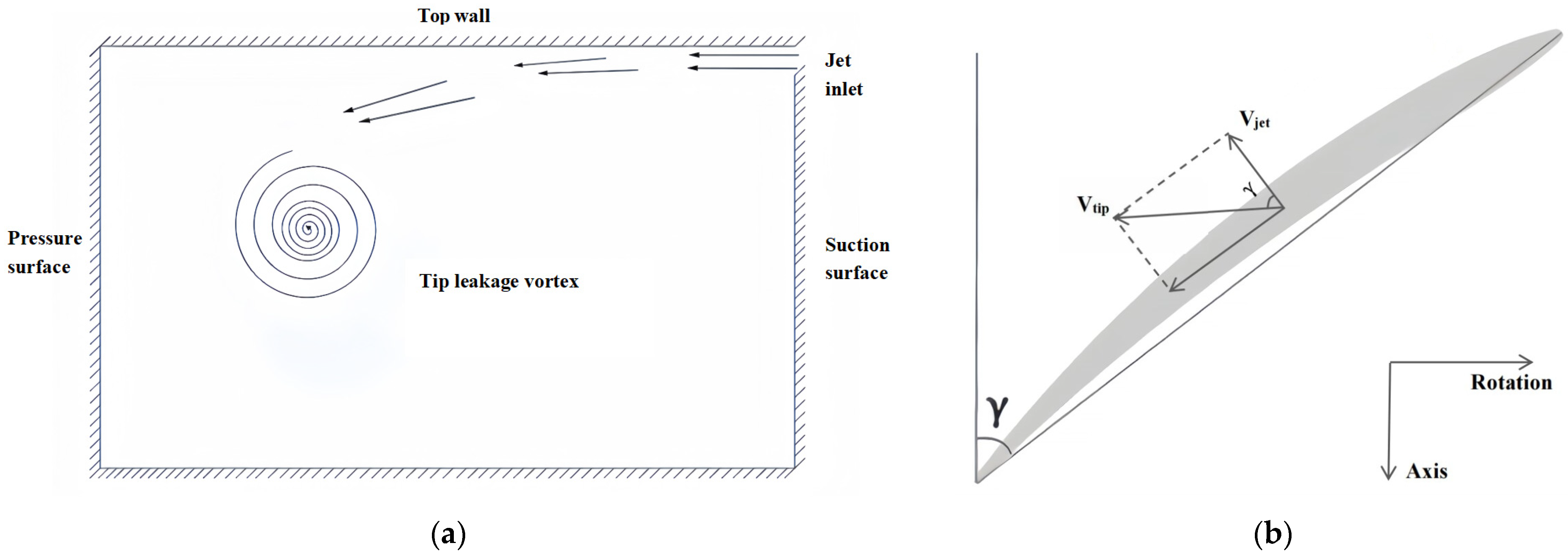
• An analysis of the main jet’s flow mixing characteristics revealed the cause of TLV formation: the lateral jets from the slot induce a blockage effect, which results in a large low-speed area; the low-speed flow gives rise to a strong momentum exchange with the originally steady mainstream, which, furthermore, forms a spiral vortex structure with a high vorticity magnitude, i.e., TLV. The instantaneous vorticity simulation is highly consistent with the experimental results, validating the reliability of the model.
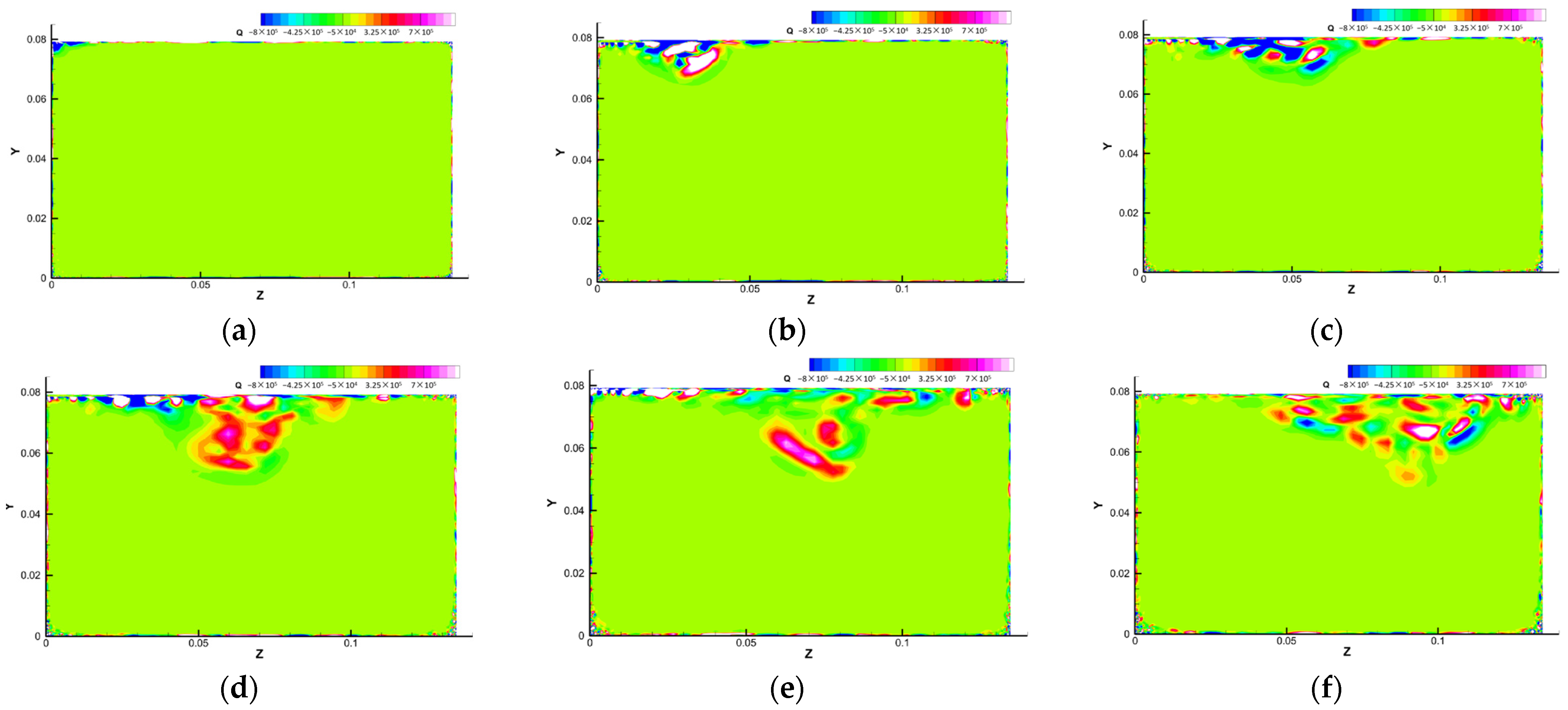
• The evolution of the TLV is divided into three main parts. The first part is the jet slot, predominantly characterized by negative vorticity flow. The second part is the TLV formation, mainly composed of significant negative streamwise vortices. The third part is the development of TLV, where positive and negative vorticities begin to interact, resulting in a more complex overall structure.
• The simplified square-cavity jet model successfully reveals the vortex structures in the tip clearance of an axial flow pump impeller, including the TLV, Corner Vortex (CV), and Induced Vortices. Clearly, the TLV is the main factor causing complex phenomena in tip leakage. The TLV forms at x/c = 1, initially dominated by concentrated negative vortices. At x/c = 1.2, the clear boundaries of positive and negative vortices are visible. As the TLV develops, it breaks down between x/c = 1.2 and 1.5, unbalancing the original stable boundaries between the positive and negative vortices. Downstream, many small-scale vortices are formed and extended, with the TLV tending to move towards the sidewall at $z_{max}$.
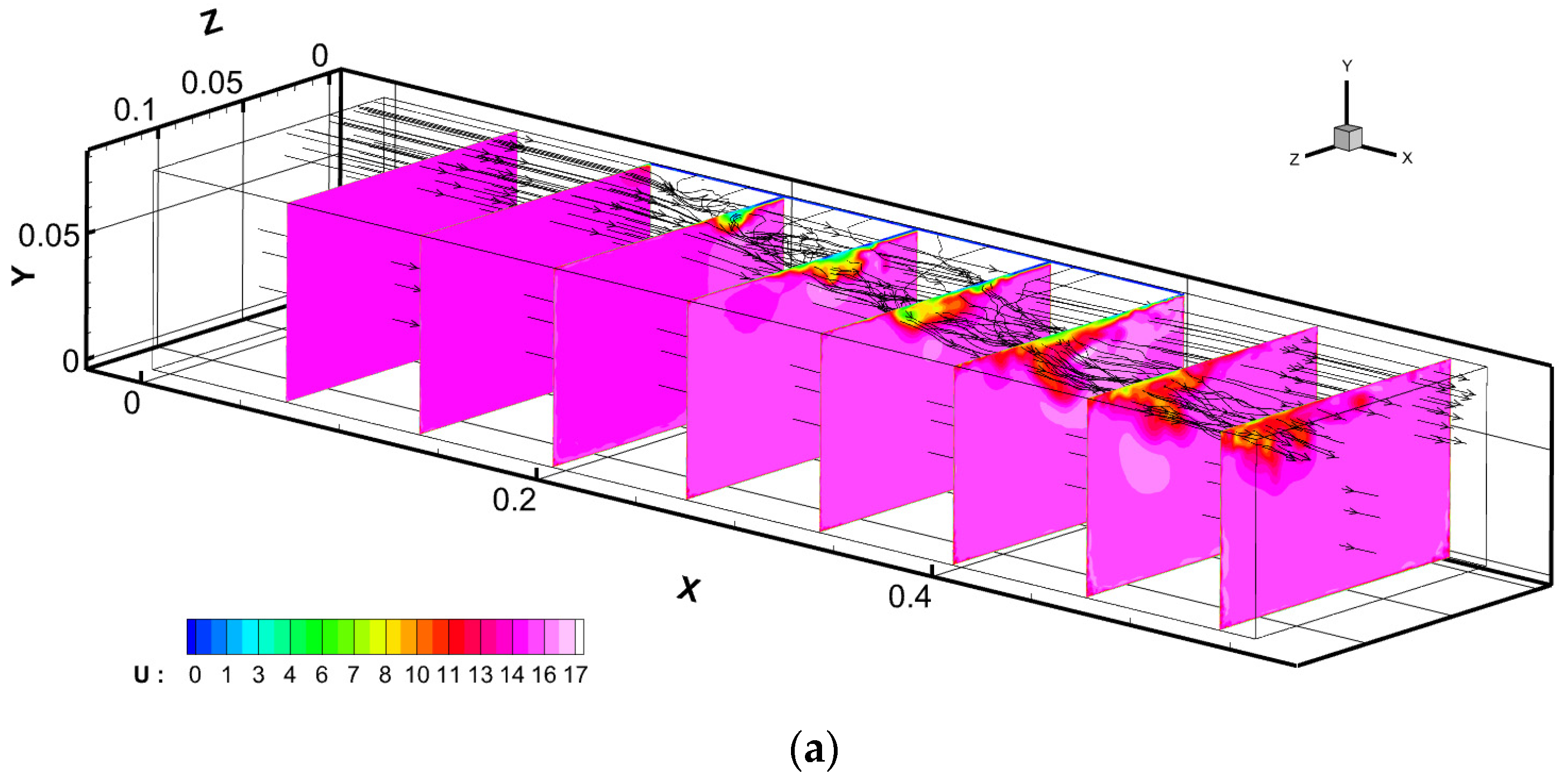
• During the initial formation of the TLV, the main stream is more stable compared to the jet. The jet streamline, positioned between the positive and negative regions of the average velocities $\langle v\rangle$ and $\langle w\rangle$, shows strong swirling characteristics. In the initial stages of TLV formation, corresponding to the second part of conclusion 2, the TLV generation area, the jet is the primary influencing factor in the flow field. As the TLV ruptures, the jet becomes more stable compared to its initial state, with the main jet’s mixing effect now playing a dominant role.

References

1. Denton, J.D. Loss Mechanisms in Turbomachines. Trans. ASME J. Turbomach. 1993, 115, V002T14A001. [Google Scholar] [CrossRef]
2. Booth, T.C.; Dodge, P.R.; Hepworth, H.K. Rotor-Tip Leakage: Part I—Basic Methodology. J. Eng. Power 1982, 104, 154–161. [Google Scholar] [CrossRef]
3. Dreyer, M.; Decaix, J.; Münch-Alligné, C.; Farhat, M. Mind the gap: A new insight into the tip leakage vortex using stereo-PIV. Exp. Fluids 2014, 55, 1849. [Google Scholar] [CrossRef]
4. Pouffary, B.; Patella, R.F.; Reboud, J.-L.; Lambert, P.-A. Numerical Simulation of 3D Cavitating Flows: Analysis of Cavitation Head Drop in Turbomachinery. J. Fluids Eng. 2008, 130, 061301. [Google Scholar] [CrossRef]
5. Doeller, N. Cavitation Breakdown in an Axial Waterjet Pump: An Experimental Characterization of Flow Phenomena. Ph.D. Thesis, Johns Hopkins University, Baltimore, MD, USA, 2017. [Google Scholar]
6. Shridhar, G.; Katz, J.; Liu, H.L. Effect of Gap Size on Tip Leakage Cavitation Inception, Associated Noise and Flow Structure. J. Fluids Eng. 2002, 124, 994–1004. [Google Scholar]
7. Choi, J.-K.; Chahine, G.L. Noise due to extreme bubble deformation near inception of tip vortex cavitation. Phys. Fluids 2004, 16, 2411–2418. [Google Scholar] [CrossRef]
8. Shi, Y.; Pan, G.; Wang, P.; Du, X. Numerical Analysis of Cavitation Characteristics of Pumpjet Propulsors. J. Shanghai Jiao Tong Univ. 2014, 48, 1059–1064. [Google Scholar]
9. Lu, L.; Pan, G. Numerical Simulation Analysis of Unsteady Cavitation Performance of Pumpjet Propulsors. J. Shanghai Jiao Tong Univ. 2015, 49, 262–268. [Google Scholar]
10. Mao, X.; Liu, B.; Tang, T.; Zhao, H. The impact of casing groove location on the flow instability in a counter-rotating axial flow compressor. Aerosp. Sci. Technol. 2018, 76, 250–259. [Google Scholar] [CrossRef]
11. Li, J.; Du, J.; Li, F.; Zhang, Q.; Zhang, H. Stability enhancement using a new hybrid casing treatment in an axial flow compressor. Aerosp. Sci. Technol. 2019, 85, 305–319. [Google Scholar] [CrossRef]
12. Tan, C.S. Three-dimensional and tip clearance flows in compressors. In Proceedings of the Von Karman Institute for Fluid Dynamics Lecture Series: Advances in Axial Compressor Aerodynamics, Ghent, Belgium, 10 July 2006. [Google Scholar]
13. Rains, D.A.; Acosta, A.J.; Rannie, W.D. Tip Clearance Flows in Axial Flow Compressors and Pumps; Hydrodynamics and Mechanical Engineering Laboratories, California Institute of Technology: Pasadena, CA, USA, 1954. [Google Scholar]
14. Booth, T.C. Importance of Tip Clearance Flows in Turbine Design, VKI Lecture Series 1985-05: Tip Clearance Effects in Axial Turbomachines; Von Karman Institute for Fluid Dynsmics: Sint-Genesius-Rode, Belgium, 1985; pp. 1–34. [Google Scholar]
15. Oweis, G.F.; Ceccio, S.L. Instantaneous and time-averaged flow fields of multiple vortices in the tip region of a ducted propulsor. Exp. Fluids 2005, 38, 615–636. [Google Scholar] [CrossRef]
16. Wu, H.; Miorini, R.L.; Tan, D.; Katz, J. Turbulence Within the Tip-Leakage Vortex of an Axial Waterjet Pump. AIAA J. 2012, 50, 2574–2587. [Google Scholar] [CrossRef]
17. Miorini, R.L.; Wu, H.; Katz, J. The Internal Structure of the Tip Leakage Vortex Within the Rotor of an Axial Waterjet Pump. J. Turbomach. 2012, 134, 031018. [Google Scholar] [CrossRef]
18. Miorini, R.L.; Wu, H.; Tan, D.; Katz, J. Three-Dimensional Structure and Turbulence Within the Tip Leakage Vortex of an Axial Waterjet Pump. In Proceedings of the ASME-JSME-KSME Joint Fluids Engineering Conference, Hamamatsu, Japan, 24–29 July 2011. [Google Scholar]
19. Wu, H.; Tan, D.; Miorini, R.L.; Katz, J. Three-dimensional flow structures and associated turbulence in the tip region of a waterjet pump rotor blade. Exp. Fluids 2011, 51, 1721–1737. [Google Scholar] [CrossRef]
20. Wu, H.; Miorini, R.L.; Katz, J. Measurements of the tip leakage vortex structures and turbulence in the meridional plane of an axial water-jet pump. Exp. Fluids 2011, 50, 989–1003. [Google Scholar] [CrossRef]
21. Chen, H. Experimental Investigations of Cavitation Breakdown in an Axial Waterjet Pump. J. Fluids Eng. 2015, 137, 317–320. [Google Scholar] [CrossRef]
22. Li, Y.; Chen, H.; Katz, J. Measurements and Characterization of Turbulence in the Tip Region of an Axial Compressor Rotor. J. Turbomach. 2017, 139, 121003. [Google Scholar] [CrossRef]
23. Chen, H.; Li, Y.; Katz, J. On the Interactions of a Rotor Blade Tip Flow with Axial Casing Grooves in an Axial Compressor Near the Best Efficiency Point. J. Turbomach. 2019, 141, 011008.1–011008.14. [Google Scholar] [CrossRef]
24. Li, Y.; Chen, H.; Tan, D.; Katz, J. Effects of Tip Clearance and Operating Conditions on the Flow Structure and Turbulence Within an Axial Compressor Rotor Passage. In Proceedings of the ASME Turbo Expo: Turbomachinery Technical Conference & Exposition, Seoul, Republic of Korea, 13–17 June 2016. [Google Scholar]
25. Chen, H.; Li, Y.; Tan, D.; Katz, J. Visualizations of Flow Structures in the Rotor Passage of an Axial Compressor at the Onset of Stall. J. Turbomach. 2017, 139, V02AT37A031. [Google Scholar] [CrossRef]
26. Li, Y.; Chen, H.; Tan, D.; Katz, J. On the Effects of Tip Clearance and Operating Condition on the Flow Structures Within an Axial Turbomachine Rotor Passage. J. Turbomach. 2019, 141, 111002. [Google Scholar] [CrossRef]
27. Gao, Y.; Liu, Y. A flow model for tip leakage flow in turbomachinery using a square duct with a longitudinal slit. Aerosp. Sci. Technol. 2019, 95, 105460. [Google Scholar] [CrossRef]
28. Fang, J.; Gao, Y.; Liu, Y.; Lu, L.; Yao, Y.; Le Ribault, C. Direct numerical simulation of a tip-leakage flow in a planar duct with a longitudinal slit. Phys. Fluids 2019, 31, 125108. [Google Scholar] [CrossRef]
29. Wells, J.B. Effects of Turbulence Modeling on RANS Simulations of Tip Vortices. In Proceedings of the AIAA Aerospace Sciences Meeting Including the New Horizons Forum & Aerospace Exposition, Orlando, FL, USA, 5–8 January 2009. [Google Scholar]
30. Zhang, D.; Pan, D.; Shi, W.; Wu, S.; Shao, P. Study on tip leakage vortex in an axial flow pump based on modified shear stress transport k-ω turbulence model. Therm. Sci. 2013, 17, 1551–1555. [Google Scholar] [CrossRef]
31. Zhang, D.; Shi, W.; Van Esch, B.B.; Shi, L.; Dubuisson, M. Numerical and experimental investigation of tip leakage vortex trajectory and dynamics in an axial flow pump. Comput. Fluids 2015, 112, 61–71. [Google Scholar] [CrossRef]
32. Decaix, J.; Balarac, G.; Dreyer, M.; Farhat, M.; Münch, C. RANS and LES computations of the tip-leakage vortex for different gap widths. J. Turbul. 2015, 16, 309–341. [Google Scholar] [CrossRef]
33. Lu, L.; Gao, Y.; Li, Q.; Du, L. Numerical investigations of tip clearance flow characteristics of a pumpjet propulsor. Int. J. Nav. Archit. Ocean Eng. 2018, 10, 307–317. [Google Scholar] [CrossRef]
34. Guan, X. Modern Pump Theory and Design; China Aerospace Publishing House: Beijing, China, 2011; pp. 40–45. [Google Scholar]
35. Hunt, J.C.; Wray, A.A.; Moin, P. Eddies, Streams, and Convergence Zones in Turbulent Flows; CTR-S88; Center for Turbulence Research Report: Stanford, CA, USA, 1988; pp. 193–208. [Google Scholar]
36. Zhou, J.; Adrian, R.J.; Balachandar, S.; Kendall, T. Mechanisms for generating coherent packets of hairpin vortices in channel flow. J Fluid Mech. Phys. Fluids 1999, 387, 353–396. [Google Scholar] [CrossRef]
37. Pirozzoli, S.; Bernardini, M.; Grasso, F. Characterization of coherent vortical structures in a supersonic turbulent boundary layer. J. Fluid Mech. 2008, 613, 205–231. [Google Scholar] [CrossRef]
Figure 1. Illustration of the structure of Tip Leakage Flow (TLF).
Water 16 00676 g001
Figure 2. Perspective view of the axial flow pump model AxWJ-1 [18]. A refers to the top and side planes of the casing, B denotes the inlet section, C represents the rotor, and D signifies the stator; Ω symbolizes the rotation axis.
Water 16 00676 g002
Figure 3. Geometric shape of the flow model. The area marked by the blue and red lines is the extracted impeller single channel.
Water 16 00676 g003
Figure 4. Definition of flow parameters: (a) schematic diagram of the model cross-section; (b) schematic representation of velocity definition.
Water 16 00676 g004
Figure 5. Grid distribution of the computational domain. The red solid lines mark the effective area, and the blue patch marks the slit.
Water 16 00676 g005
Figure 6. Instantaneous flow field in the z-y plane: (a) streamwise velocity u; (b) spanwise velocity w; (c) streamlines; (d) streamwise vorticity.
Water 16 00676 g006aWater 16 00676 g006b
Figure 7. Visualization of instantaneous turbulent coherent structures of the model t = 0.2442   s : (a) isosurfaces based on the λ c i criterion, (b) isosurfaces based on the Q criterion.
Water 16 00676 g007
Figure 8. Visualization of instantaneous turbulent coherent structures on the y = y max isosurface: (a) 1.99 y y max , (b) 1.98 y y max , (c) 1.95 y y max .
Water 16 00676 g008aWater 16 00676 g008b
Figure 9. Evolution of instantaneous streamwise vorticity in plane z-y.
Water 16 00676 g009
Figure 10. Instantaneous streamwise vorticity in cross section z-y: (a) x/c = 1; (b) x/c = 1.5; (c) x/c = 2; (d) x/c = 2.5; (e) x/c = 3; (f) x/c = 3.5.
Water 16 00676 g010
Figure 11. The average flow field in the X-direction: (a) vortex streamline diagram; (b) vortex identification map.
Water 16 00676 g011
Figure 12. Time-average velocity and streamlines in the z-y plane: (a) average streamwise velocity u ; (b) average y-direction velocity v ; (c) average z-direction velocity w .
Water 16 00676 g012aWater 16 00676 g012b
Figure 13. Streamlines (a) and the distribution of average velocities: u (b), v (c), and w (d).
Water 16 00676 g013