
Fault Diagnosis in Hydroelectric Units in Small-Sample State Based on Wasserstein Generative Adversarial Network


Abstract
1. Introduction
- (1)
- Aiming to solve the problem of fewer sample data for hydropower unit faults, we propose the W-GAN hydropower unit data augmentation approach;
- (2)
- We effectively expand the sample features and improve the accuracy of fault diagnosis;
- (3)
- For cases in which the training data are sufficiently small or the sample features are single, we make full use of the data generated through the W-GAN training process Generator in different epochs, combining them with the actual data to enrich the sample features.
2. Theoretical Background
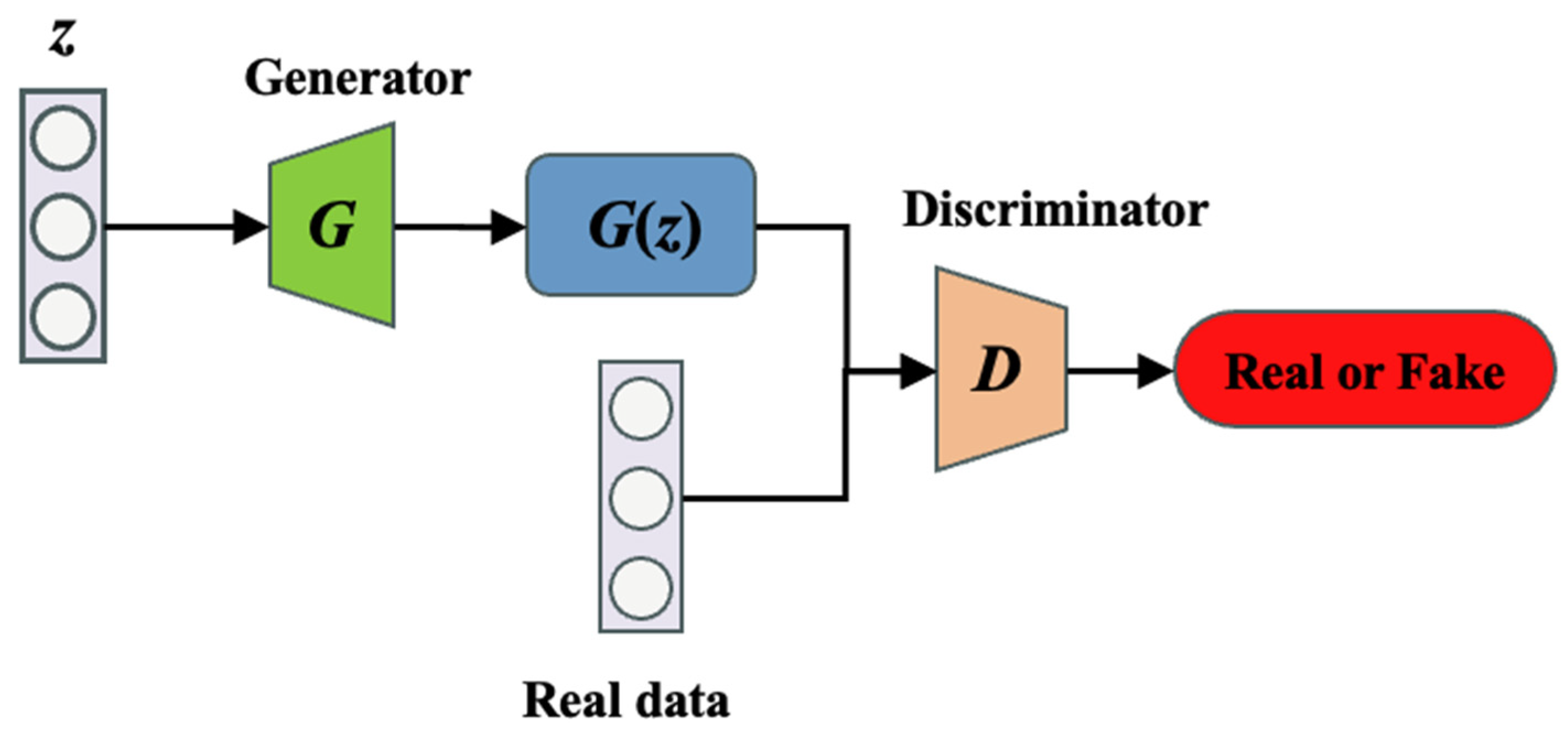
2.1. W-GAN
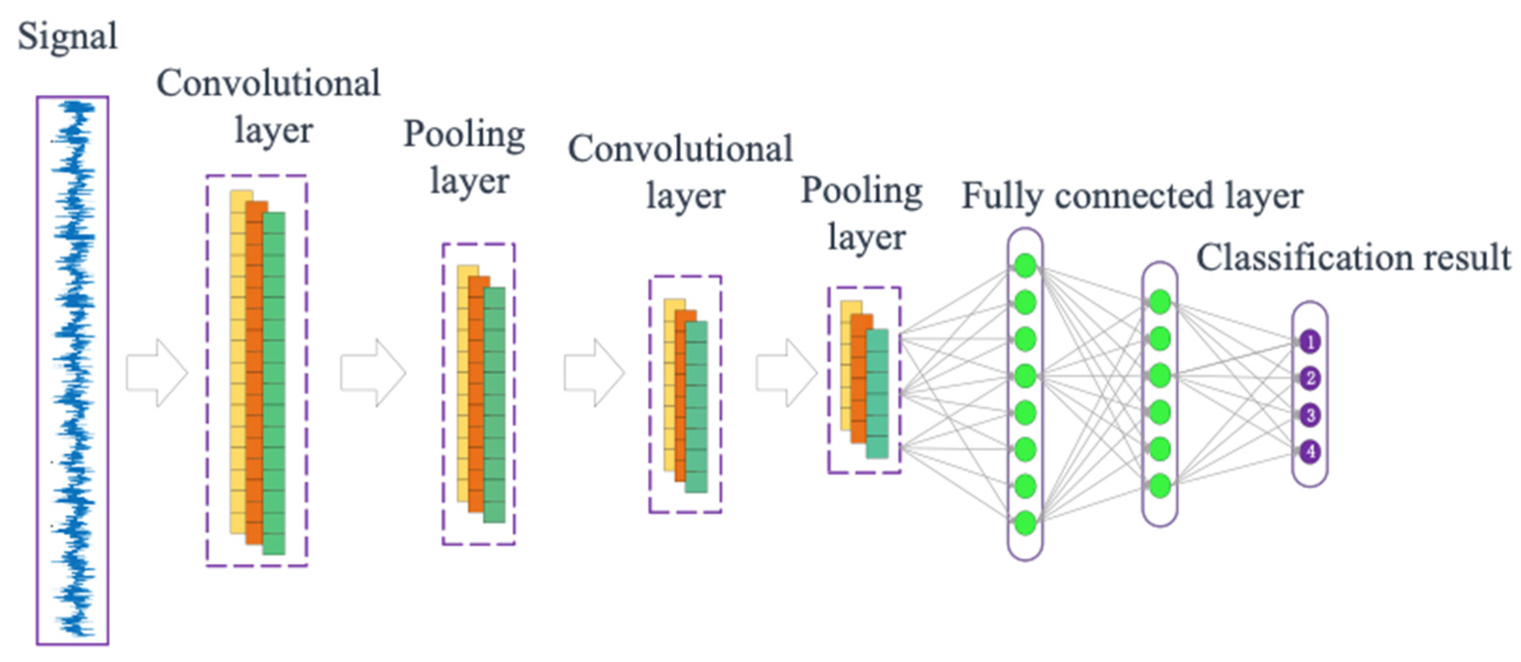
2.2. 1D-CNN
3. Proposed Method
- The collection of vibration waveform data from mechanical vibrations associated with hydroelectric units using sensors;
- The zero-mean preprocessing of collected data on different fault types in hydroelectric units;
- The preprocessed waveform data are converted to frequency domain via FFT, and the spectrum is obtained;
- The spectral dataset is divided into a training set and a test set according to the proportion of unbalanced small-sample states, where the training set is used to train W-GAN and the test set is used to validate the model for fault diagnosis;
- We train W-GAN using the training set, obtain the data generated via W-GAN in different epochs, and expand the dataset for the training set;
- The expanded dataset trains 1D-CNN, and the test set is inputted to 1D-CNN for fault diagnosis.
4. Experimental Verification
4.1. Introduction of Experimental Data
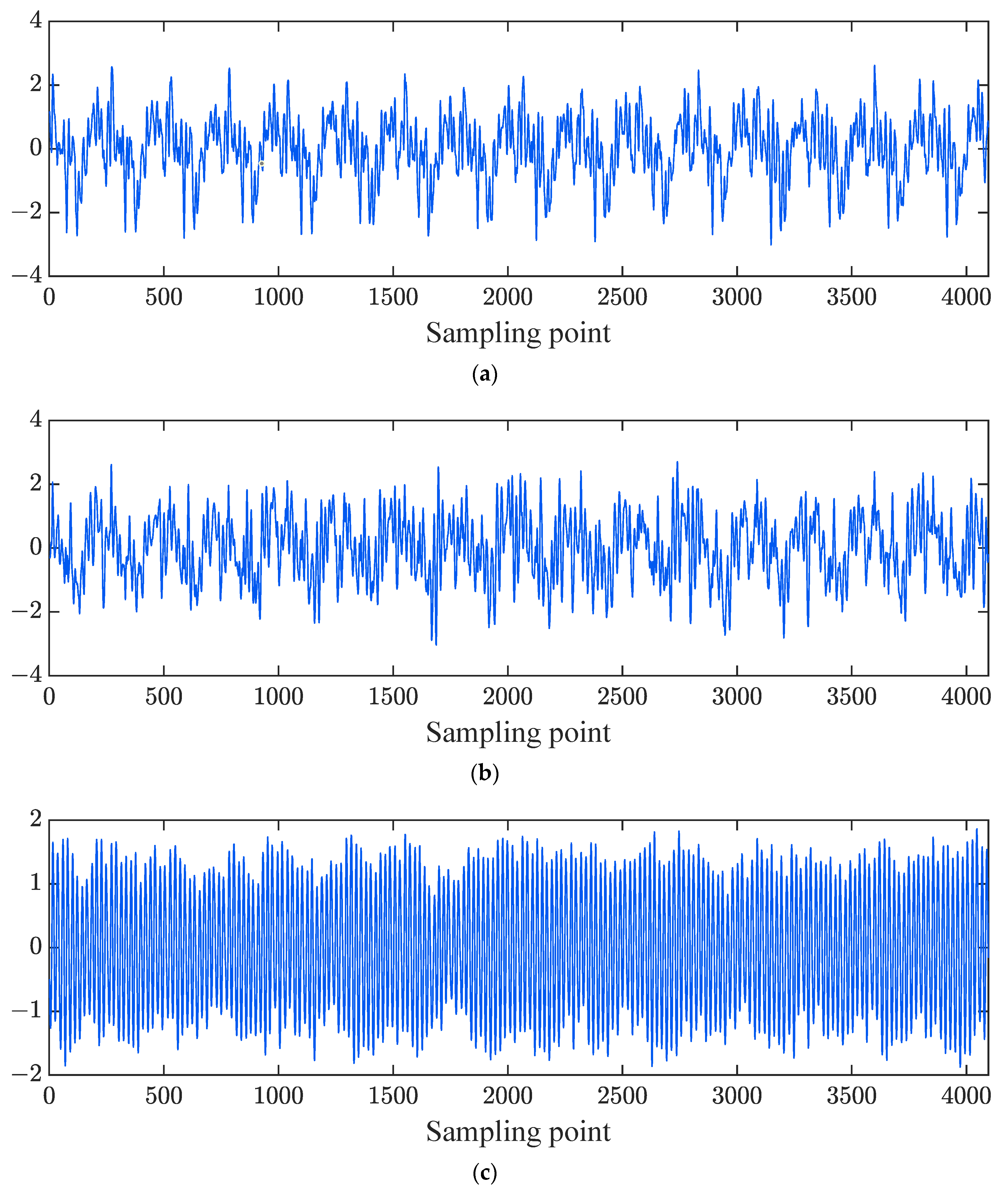
4.2. Data Preprocessing
- (a)
- Zero-mean normalization
- (b) Fourier Transform
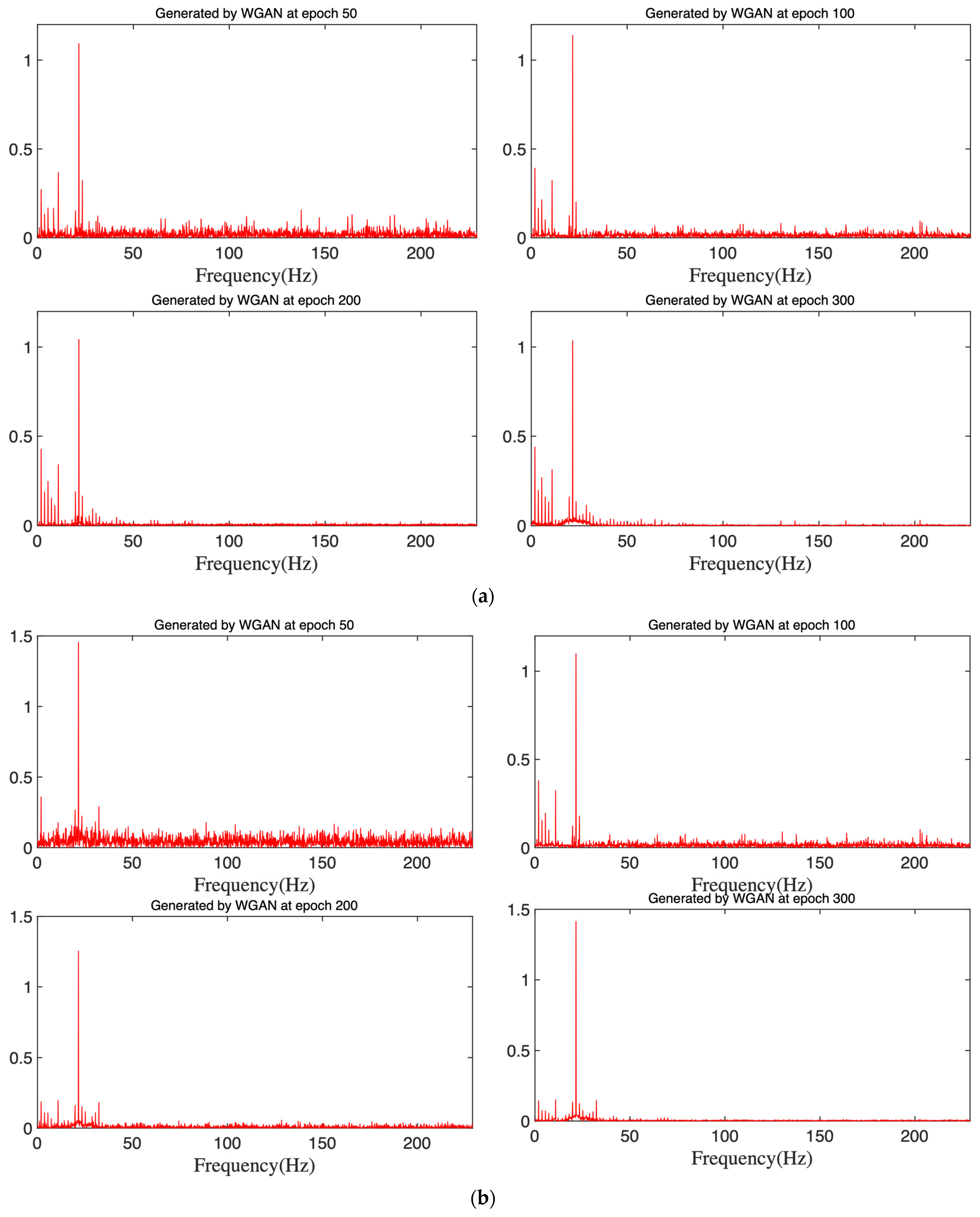
4.3. Data Augmentation Based on W-GAN
4.4. Evaluation of the Data Generated
- (a)
- PCC
- (b)
- Cosine similarity
4.5. Fault Diagnosis and Result Analysis
5. Conclusions
- The small-sample fault diagnosis method based on W-GAN proposed in this paper realizes the augmentation of small-sample hydropower unit imbalance data by combining the fault data of the No. 3 hydropower unit of a power station in China. The results show that the features of the enhanced samples are more abundant. The accuracy of fault diagnosis has been improved by 7% on average compared with that of the unenhanced fault diagnosis;
- By combining the data generated by W-GAN in different iterations with the actual data, it was found that the more iterations of the model, the richer the sample features, and the higher the accuracy in CNN troubleshooting identification.
Author Contributions
Funding
Data Availability Statement
Conflicts of Interest
References
- de Santis, R.B.; Costa, M.A. Extended isolation forests for fault detection in small hydroelectric plants. Sustainability 2020, 12, 6421. [Google Scholar] [CrossRef]
- Yuan, Z.; Xiong, G.; Fu, X. Artificial Neural Network for Fault Diagnosis of Solar Photovoltaic Systems: A Survey. Energies 2022, 15, 8693. [Google Scholar] [CrossRef]
- Chen, Q.; Han, Y.; Wu, J.; Gan, Y. Energy-Saving Task Scheduling Based on Hard Reliability Requirements: A Novel Approach with Low Energy Consumption and High Reliability. Sustainability 2022, 14, 6591. [Google Scholar] [CrossRef]
- Tian, H.; Yang, L.; Ji, P. Intelligent Analysis of Vibration Faults in Hydroelectric Generating Units Based on Empirical Mode Decomposition. Processes 2023, 11, 2040. [Google Scholar] [CrossRef]
- Dao, F.; Zeng, Y.; Zou, Y.; Li, X.; Qian, J. Acoustic vibration approach for detecting faults in hydroelectric units: A review. Energies 2021, 14, 7840. [Google Scholar] [CrossRef]
- Liao, G.-P.; Gao, W.; Yang, G.-J.; Guo, M.-F. Hydroelectric generating unit fault diagnosis using 1-D convolutional neural network and gated recurrent unit in small hydro. IEEE Sens. J. 2019, 19, 9352–9363. [Google Scholar] [CrossRef]
- Zhang, F.; Guo, J.; Yuan, F.; Shi, Y.; Li, Z. Research on Denoising Method for Hydroelectric Unit Vibration Signal Based on ICEEMDAN–PE–SVD. Sensors 2023, 23, 6368. [Google Scholar] [CrossRef] [PubMed]
- Yao, Q.; Liu, Y. Vibration fault diagnosis of hydroelectric unit based on LS-SVM and information fusion technology. In Proceedings of the 2016 4th International Conference on Electrical & Electronics Engineering and Computer Science (ICEEECS 2016), Jinan, China, 15–16 October 2016; Atlantis Press: Amsterdam, The Netherlands, 2016; pp. 720–725. [Google Scholar]
- Attoui, I.; Boutasseta, N.; Fergani, N.; Oudjani, B.; Deliou, A. Vibration-based bearing fault diagnosis by an integrated DWT-FFT approach and an adaptive neuro-fuzzy inference system. In Proceedings of the 2015 3rd International Conference on Control, Engineering & Information Technology (CEIT), Tlemcen, Algeria, 25–27 May 2015; IEEE: Piscataway, NJ, USA, 2015; p. 16. [Google Scholar]
- Zhang, Q.; Deng, L. An intelligent fault diagnosis method of rolling bearings based on short-time Fourier transform and convolutional neural network. J. Fail. Anal. Prev. 2023, 23, 795–811. [Google Scholar] [CrossRef]
- Kolar, D.; Lisjak, D.; Pająk, M.; Gudlin, M. Intelligent fault diagnosis of rotary machinery by convolutional neural network with automatic hyper-parameters tuning using Bayesian optimization. Sensors 2021, 21, 2411. [Google Scholar] [CrossRef] [PubMed]
- Wang, Y.; Zou, Y.; Hu, W.; Chen, J.; Xiao, Z. Intelligent fault diagnosis of hydroelectric units based on radar maps and improved GoogleNet by depthwise separate convolution. Meas. Sci. Technol. 2023, 35, 025103. [Google Scholar] [CrossRef]
- Yu, G.; You, Y.; Ma, B.; Han, Y. Intelligent Fault Diagnosis for Unknown Faults of Rotating Machinery based on the CNN and the DCGAN. In Proceedings of the 2023 IEEE 12th Data Driven Control and Learning Systems Conference (DDCLS), Xiangtan, China, 12–14 May 2023; IEEE: Piscataway, NJ, USA, 2023; pp. 72–77. [Google Scholar]
- Gao, Y.; Chai, C.; Li, H.; Fu, W. A deep learning framework for intelligent fault diagnosis using AutoML-CNN and image-like data fusion. Machines 2023, 11, 932. [Google Scholar] [CrossRef]
- Mushtaq, S.; Islam, M.M.; Sohaib, M. Deep learning aided data-driven fault diagnosis of rotatory machine: A comprehensive review. Energies 2021, 14, 5150. [Google Scholar] [CrossRef]
- Zhang, X.; Wang, H.; Wu, B.; Zhou, Q.; Hu, Y. A novel data-driven method based on sample reliability assessment and improved CNN for machinery fault diagnosis with non-ideal data. J. Intell. Manuf. 2023, 34, 2449–2462. [Google Scholar] [CrossRef]
- Zhang, X.; Wu, P.; He, J.; Lou, S.; Gao, J. A gan based fault detection of wind turbines gearbox. In Proceedings of the 2020 7th International Conference on Information, Cybernetics, and Computational Social Systems (ICCSS), Guangzhou, China, 13–15 November 2020; IEEE: Piscataway, NJ, USA, 2020; pp. 271–275. [Google Scholar]
- Yang, J.; Liu, J.; Xie, J.; Wang, C.; Ding, T. Conditional GAN and 2-D CNN for bearing fault diagnosis with small samples. IEEE Trans. Instrum. Meas. 2021, 70, 3525712. [Google Scholar] [CrossRef]
- Chen, B. A Research on Fault Diagnosis of Wind Turbine CMS Based on Bayesian-GAN-LSTM Neural Network. J. Phys. Conf. Ser. 2022, 2417, 012031. [Google Scholar] [CrossRef]
- Goodfellow, I.; Pouget-Abadie, J.; Mirza, M.; Xu, B.; Warde-Farley, D.; Ozair, S.; Courville, A.; Bengio, Y. Generative adversarial nets. In Proceedings of the Advances in Neural Information Processing Systems 27 (NIPS 2014), Montreal, QC, Canada, 8–13 December 2014. [Google Scholar]
- Barua, S.; Erfani, S.M.; Bailey, J. FCC-GAN: A fully connected and convolutional net architecture for GANs. arXiv 2019, arXiv:1905.02417. [Google Scholar]
- Eren, L.; Ince, T.; Kiranyaz, S. A generic intelligent bearing fault diagnosis system using compact adaptive 1D CNN classifier. J. Signal Process. Syst. 2019, 91, 179–189. [Google Scholar] [CrossRef]
- Pandian, R.; Sabarivani, A.; Ramadevi, R.; Krishnamoorthy, N. Effect of data preprocessing in the detection of epilepsy using machine learning techniques. J. Sci. Ind. Res. 2022, 80, 1066–1077. [Google Scholar]


| Term | Symbol | Definition | Function |
|---|---|---|---|
| Noise Vector | z | A randomly generated vector that serves as input to the generator | Provides an initial point for the generator to produce data |
| Generator | G | A model, typically a neural network, that accepts a noise vector and produces data | Learns to create new data instances that increasingly resemble the true data distribution |
| Generated Data | G(z) | The data produced by the generator based on the input noise vector z | Intended to deceive the discriminator into believing that the data are authentic |
| Discriminator | D | A model, often a neural network, that assesses whether input data are authentic or fabricated by the generator | Learns to distinguish between fake data generated by the generator and real data, thereby improving its accuracy in judgement |
| Training Set | Test Set | |||||
|---|---|---|---|---|---|---|
| Class 1 | Class 2 | Class 3 | Class 1 | Class 2 | Class 3 | |
| Number of samples | 20 | 10 | 10 | 20 | 20 | 20 |
| Percentage | 50 | 25 | 25 | 33.33 | 33.33 | 33.33 |
| Total number of samples | 40 | 60 | ||||
| Overall percentage | 40 | 60 | ||||
| # | Network Layer | Input Size | Output Size | Activation Layer |
|---|---|---|---|---|
| Generator: | ||||
| 1 | Linear layer 1 | 200 | 500 | LeakyRelu |
| 2 | Linear layer 2 | 500 | 1000 | LeakyRelu |
| 3 | Linear layer 3 | 1000 | 2048 | LeakyRelu |
| Discriminator: | ||||
| 4 | Convolutional layer 1 | [1, 2048] | [4, 2048] | LeakyRelu |
| 5 | Pooling layer | [1, 2048] | [4, 1024] | |
| 6 | Convolutional layer 2 | [4, 1024] | [4, 1024] | LeakyRelu |
| 7 | Pooling layer | [4, 1024] | [4, 512] | |
| 8 | Fully connected layer 1 | [1, 2048] | [1, 256] | LeakyRelu |
| 9 | Fully connected layer 2 | [1, 256] | [1, 1] | Sigmoid |
| Epoch | PCC | CS | ||||||
|---|---|---|---|---|---|---|---|---|
| 50 | 100 | 200 | 300 | 50 | 100 | 200 | 300 | |
| Class 2 | 0.742 | 0.875 | 0.915 | 0.988 | 0.675 | 0.919 | 0.914 | 0.969 |
| Class 3 | 0.693 | 0.781 | 0.937 | 0.977 | 0.713 | 0.827 | 0.912 | 0.939 |
| Epoch | Training Set | Test Set | |||||
|---|---|---|---|---|---|---|---|
| Class 1 | Class 2 | Class 3 | Class 1 | Class 2 | Class 3 | ||
| Group 1 | / | 20 | 10 | 10 | 20 | 20 | 20 |
| Group 2 | 100 | 20 | 20 | 20 | 20 | 20 | 20 |
| Group 3 | 200 | 20 | 20 | 20 | 20 | 20 | 20 |
| Group 4 | 300 | 20 | 20 | 20 | 20 | 20 | 20 |
| # | Network Layer | Parameters | Output Size |
|---|---|---|---|
| 1 | Input layer | / | [1, 2048] |
| 2 | Convolutional layer | Input Channels: 1; Output Channels: 32 Kernel Size: 3 × 1; Stride: 1 | [32, 2048] |
| 3 | Batch normalization layer | / | [32, 2048] |
| 4 | Pooling layer | Kernel Size: 2 × 1; Stride: 2 | [32, 1024] |
| 5 | Convolutional layer | Input Channels: 32; Output Channels: 4; Kernel Size: 3 × 1; | [4, 1024] |
| 6 | Batch normalization layer | / | [4, 1024] |
| 7 | Pooling layer | Kernel Size: 2 × 1; Stride: 2 | [4, 512] |
| 8 | Flatten layer | / | [1, 2048] |
| 9 | Fully connected layer 1 | Input Channels: 2048, Output Channels: 512 | [1, 512] |
| 10 | Fully connected layer 2 | Input Channels: 512, Output Channels: 32 | [1, 32] |
| 11 | Fully connected layer 3 | Input Channels: 32, Output Channels: 3 | [1, 3] |
| Model | Datasets Used | Number of Samples in the Training Set after Data Augmentation | Average Accuracy |
|---|---|---|---|
| Proposed method (GAN-1D-CNN) | Group 4 | 60 | 89.12 |
| GAN-BPNN | Group 4 | 60 | 84.42 |
| SVM | Group 1 | 40 | 67.12 |
| 1D-CNN | Group 1 | 40 | 81.36 |
| BPNN | Group 1 | 40 | 75.28 |
Disclaimer/Publisher’s Note: The statements, opinions and data contained in all publications are solely those of the individual author(s) and contributor(s) and not of MDPI and/or the editor(s). MDPI and/or the editor(s) disclaim responsibility for any injury to people or property resulting from any ideas, methods, instructions or products referred to in the content. |
© 2024 by the authors. Licensee MDPI, Basel, Switzerland. This article is an open access article distributed under the terms and conditions of the Creative Commons Attribution (CC BY) license (https://creativecommons.org/licenses/by/4.0/).
Share and Cite
Sun, W.; Zou, Y.; Wang, Y.; Xiao, B.; Zhang, H.; Xiao, Z. Fault Diagnosis in Hydroelectric Units in Small-Sample State Based on Wasserstein Generative Adversarial Network. Water 2024, 16, 454. https://doi.org/10.3390/w16030454
Sun W, Zou Y, Wang Y, Xiao B, Zhang H, Xiao Z. Fault Diagnosis in Hydroelectric Units in Small-Sample State Based on Wasserstein Generative Adversarial Network. Water. 2024; 16(3):454. https://doi.org/10.3390/w16030454
Chicago/Turabian StyleSun, Wenhao, Yidong Zou, Yunhe Wang, Boyi Xiao, Haichuan Zhang, and Zhihuai Xiao. 2024. "Fault Diagnosis in Hydroelectric Units in Small-Sample State Based on Wasserstein Generative Adversarial Network" Water 16, no. 3: 454. https://doi.org/10.3390/w16030454
APA StyleSun, W., Zou, Y., Wang, Y., Xiao, B., Zhang, H., & Xiao, Z. (2024). Fault Diagnosis in Hydroelectric Units in Small-Sample State Based on Wasserstein Generative Adversarial Network. Water, 16(3), 454. https://doi.org/10.3390/w16030454