Integrating Convolutional Attention and Encoder–Decoder Long Short-Term Memory for Enhanced Soil Moisture Prediction

Abstract

Soil moisture is recognized as a crucial variable in land–atmosphere interactions. This study introduces the Convolutional Attention Encoder–Decoder Long Short-Term Memory (CAEDLSTM) model to address the uncertainties and limitations inherent in traditional soil moisture prediction methods, especially in capturing complex temporal dynamics across diverse environmental conditions. Unlike existing approaches, this model integrates convolutional layers, an encoder–decoder framework, and multi-head attention mechanisms for the first time in soil moisture prediction. The convolutional layers capture local spatial features, while the encoder–decoder architecture effectively manages temporal dependencies. Additionally, the multi-head attention mechanism enhances the model’s ability to simultaneously focus on multiple key influencing factors, ensuring a comprehensive understanding of complex environmental variables. This synergistic combination significantly improves predictive performance, particularly in challenging climatic conditions. The model was validated using the LandBench1.0 dataset, which includes multiple high-resolution datasets, such as ERA5-land, ERA5 atmospheric variables, and SoilGrids, covering various climatic regions, including high latitudes, temperate zones, and tropical areas. The superior performance of the CAEDLSTM model is evidenced by comparisons with advanced models such as AEDLSTM, CNNLSTM, EDLSTM, and AttLSTM. Relative to the traditional LSTM model, CAEDLSTM achieved an average increase of 5.01% in R², a 12.89% reduction in RMSE, a 16.67% decrease in bias, and a 4.35% increase in KGE. Moreover, it effectively addresses the limitations of traditional deep learning methods in challenging climates, including tropical Africa, the Tibetan Plateau, and Southeast Asia, resulting in significant enhancements in predictive accuracy within these regions, with R² values improving by as much as 20%. These results underscore the capabilities of CAEDLSTM in capturing complex soil moisture dynamics, demonstrating its considerable potential for applications in agriculture and water resource monitoring across diverse climates.

1. Introduction

Soil moisture is an important factor that connects atmospheric processes with land surface conditions. It plays a vital role in climate, hydrological cycles, and ecosystems. Soil moisture is essential for various applications, including weather forecasting, flood assessment, and agricultural management [1,2,3]. The regulation of surface energy and water exchanges by soil moisture influences evaporation and transpiration, directly affecting atmospheric moisture content and temperature distribution [4]. This control not only impacts local weather but also exerts a broader influence on climate by altering cloud formation and precipitation patterns [5]. As a key component of the climate system, soil moisture governs the surface energy balance and water cycling, significantly affecting seasonal climate variations and extreme weather events such as droughts and floods [6]. Within the hydrological cycle, soil moisture dictates the partitioning of precipitation, influencing surface runoff, infiltration, and groundwater recharge [7]. In ecosystems, soil moisture has a direct impact on plant growth, water use efficiency, and biodiversity, thereby determining the health and stability of ecosystems [8]. Accurate measurement and prediction of soil moisture are critical for improving the accuracy of weather forecasts, assessing flood risks, and optimizing agricultural irrigation strategies [9]. This study focuses on the development of short-term (1-day lead time) soil moisture prediction models to address these challenges.

Over the past decades, soil moisture prediction has predominantly been reliant on process-based models, such as land surface and hydrological models. These models utilize parameterization schemes to simulate soil hydrological processes, incorporating factors such as topography and soil type [10]. Notable examples include the SWAT model for watershed-scale applications [11], the HYDRUS model for unsaturated zone water movement [12], and the MODFLOW model for groundwater flow [13]. However, these approaches are subject to significant limitations, including uncertainties in driving factors, high computational demands, and challenges in accurately capturing the nonlinear characteristics of land–atmosphere interactions [14]. Consequently, prediction accuracy and model applicability are persistently challenging.

With advancements in computational power and the increasing availability of extensive datasets in Earth sciences, data-driven machine learning and deep learning models have been shown to exhibit exceptional performance in hydrological prediction. These models learn directly from data, thereby circumventing the need for problem-specific theories or assumptions. A variety of machine learning algorithms have been applied in this context. For instance, Support Vector Machines (SVMs) and Relevance Vector Machines (RVMs) were utilized by Hong et al. [15] to develop a novel site-specific soil moisture prediction framework, which maintained high accuracy over a sustained period of one year. Zhao et al. [16] devised a soil moisture relationship model using the Random Forest approach, leveraging MODIS and AMSR-E products to address the limitations imposed by the coarse spatial resolution of passive microwave soil moisture products. Qiu et al. [17] developed a multivariate linear regression (MLR) model to predict spatial patterns, incorporating land use and topographic indices, and assessed its performance and applicability to soil moisture in the Loess Plateau. Model prediction accuracy was enhanced by Mabunga et al. [18] through the use of Gaussian process regression for model development and Bayesian optimization for hyperparameter tuning. Elshorbagy et al. [19] found that artificial neural network (ANN) models demonstrate high performance in identifying crucial state variables and predicting soil moisture levels, although they are influenced by the structure and composition of soil cover.

Compared to conventional machine learning models, deep learning models are capable of transforming low-level information (raw input) into higher-level features by learning complex nonlinear functions [20]. Characterized by their adaptability and efficiency in data processing and feature extraction, deep learning models can autonomously manage missing data and noise, thereby extracting meaningful features from diverse data sources. The Long Short-Term Memory (LSTM) architecture has gained significant popularity and demonstrated considerable performance advantages in soil moisture prediction, representing a substantial advancement in predictive accuracy [21]. A regional soil moisture prediction system was developed by Filipović et al. [22] using an LSTM neural network, which outperformed traditional methods in forecasting soil moisture three days ahead with minimal errors. This model is intended to serve as a cornerstone for irrigation scheduling in AgroSense.rs, Serbia’s national digital agriculture platform. By utilizing regional data without the need for explicit definitions of hydrological processes, LSTM offers a more accurate and robust solution for predicting streamflow. It was demonstrated by Arsenault et al. [23] that LSTM networks significantly outperform traditional hydrological models in streamflow prediction for ungauged basins. An enhanced LSTM model was developed by Fang et al. [24], incorporating a novel data integration kernel to assimilate irregular SMAP observations for near-real-time soil moisture forecasting. This method surpassed existing models by reducing errors associated with unmodeled processes and forcing conditions, providing a new data-driven approach in geosciences. Additionally, a multi-head LSTM model was created by Datta et al. [25], which improves long-term soil moisture prediction by aggregating data across different time scales. This method achieves a high R-squared value of 95.04% for forecasts extending up to one month, effectively overcoming the limitations of standard LSTM models in extended predictions.

In time series prediction tasks, while LSTM networks have been widely adopted for their remarkable ability to capture long-term dependencies, they still face significant challenges when handling complex and dynamic datasets. First, while LSTMs are highly effective at capturing long-term dependencies, they often struggle to accurately capture short-term local patterns, especially in time series data with rapid fluctuations or complex multi-scale variations. The lack of localized feature extraction mechanisms can limit their ability to model high-frequency patterns [26]. Second, despite their gate mechanisms, LSTMs can still suffer from the vanishing gradient problem during training, particularly when modeling very long sequences, which hinders their ability to learn effectively over extended periods [27]. Finally, LSTMs are prone to overfitting or underfitting when faced with highly dynamic or limited datasets, as they may over-rely on irrelevant time steps. This issue is exacerbated by the absence of mechanisms to selectively focus on important features, especially in cases where the data exhibit significant variation or noise [28].

Soil moisture prediction presents unique challenges due to its sensitivity to various dynamic environmental factors, including rainfall, temperature fluctuations, and soil structure variations [29]. These factors often interact in highly nonlinear ways, and their dependencies evolve significantly over time. As these interactions become increasingly intricate, traditional Long Short-Term Memory (LSTM) models, although capable of handling temporal dependencies to some extent, frequently struggle to manage the multi-dimensional dynamics inherent in such data [30]. Advanced models such as CNN-LSTM, EDLSTM, and AttLSTM have specific limitations. For example, while CNN-LSTM uses convolutional layers for feature extraction, it often struggles to maintain the contextual relevance of earlier time steps, especially in highly dynamic environments. This issue can impede its ability to accurately capture essential temporal patterns. On the other hand, EDLSTM and AttLSTM, despite their efforts to enhance focus on relevant features, remain vulnerable to noise within the data. This susceptibility can undermine the effectiveness of their attention mechanisms, resulting in inconsistencies when identifying critical features. As a result, this limitation can hinder their ability to effectively capture the temporal features needed for accurate future predictions.

To address these challenges, we propose a model that integrates CNN, an encoder–decoder LSTM architecture, and multi-head attention mechanisms. The CNN layers act as temporal feature extractors, capturing short-term dependencies across selected time steps and reducing dimensionality while preserving critical information. The encoder–decoder LSTM structure effectively models both short- and long-term dependencies, overcoming standard LSTM limitations by enhancing the model’s ability to handle complex temporal patterns and varying sequence lengths. This design mitigates vanishing gradients and improves generalization. The multi-head attention mechanism further boosts performance by dynamically focusing on key features across time steps, enhancing the model’s handling of multi-scale and nonlinear data while reducing overfitting risks. These enhancements enable our model to significantly outperform traditional approaches in complex time series tasks, resulting in notable gains in prediction accuracy and broader applicability.

This study aims to significantly enhance the accuracy and robustness of soil moisture prediction using the CAEDLSTM model. Specifically, the goal is to address the shortcomings of existing methods in handling multi-dimensional dynamic environmental data while demonstrating the model’s strong adaptability across various climatic conditions and regional environments. Additionally, comparisons with traditional machine learning methods (such as Random Forest) and other deep learning models (e.g., CNN-LSTM, EDLSTM, and AttLSTM) will be conducted to validate the advantages and practical applicability of CAEDLSTM in real-world scenarios.

The paper is structured as follows: Section 2 outlines the Materials and Methods, detailing the datasets utilized (e.g., LandBench1.0, ERA5, and SoilGrids) and describing the architecture of the CAEDLSTM model, including its components such as LSTM, CNN, encoder–decoder structure, and attention mechanisms. Section 3 presents the Results, comparing the performance of CAEDLSTM with that of other state-of-the-art models, including AEDLSTM [31], EDLSTM [32], AttLSTM [33], CNNLSTM [34], and LSTM [35], using key metrics such as R², RMSE, and bias. This section offers insights into the model’s predictive accuracy and stability across diverse regions and climatic conditions. Section 4 provides a Discussion, analyzing the advantages and limitations of CAEDLSTM while suggesting potential improvements for future research. Finally, Section 5 concludes with a concise summary of the study’s key findings, the practical implications of the CAEDLSTM model in real-world applications, and directions for future work.

2. Materials and Methods

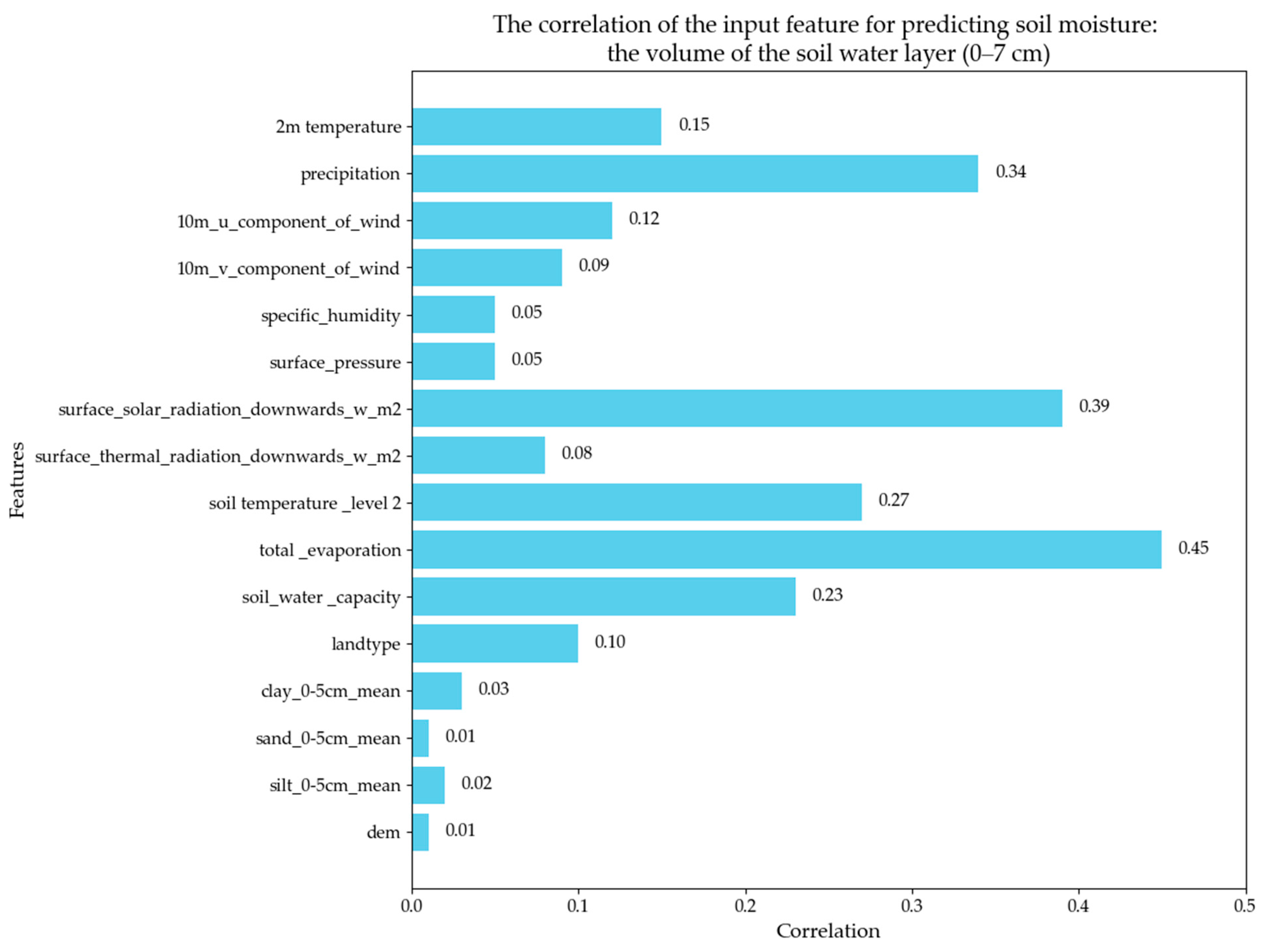
2.1. Data Description

Evaluations and comparisons were conducted utilizing the LandBench1.0 dataset, a standardized platform for predicting land surface variables (LSVs) [36,37,38]. The LSVs are derived from the ERA5-land reanalysis dataset, with atmospheric forcing variables sourced from the ERA5 reanalysis dataset and static variables obtained from the SoilGrids dataset. Soil water content was extracted from the work of Xie et al. [39], while vegetation cover types were derived from Friedl et al. [40]. The ERA5 dataset, provided by the European Centre for Medium-Range Weather Forecasts (ECMWF), represents a significant advancement over the ERA-Interim dataset, offering higher spatial resolution and increased data points [41]. In contrast, ERA5-land aims to enhance estimates of land surface states and fluxes [42]. The SoilGrids project utilizes advanced machine-learning techniques to create medium-resolution global soil property maps with a cell size of 250 m. This project integrates soil observation data and environmental descriptors from around 240,000 sites worldwide, incorporating over 400 variables related to vegetation, topography, climate, geology, and hydrology [43]. Data from SoilGrids, ERA5, and ERA5-land are extensively utilized across various research fields, providing critical soil and meteorological information to researchers and policymakers, thereby aiding in the understanding and management of challenges related to changes in the Earth system [44,45]. Furthermore, the LandBench1.0 dataset offers multiple resolution options, including 0.5°, 1°, 2°, and 4°. In this study, a resolution of 1° was selected, striking an optimal balance between computational efficiency and spatial accuracy. This resolution provides sufficient detail for representing land surface variables while significantly reducing computational demands, making it ideal for large-scale, long-term climate modeling and analysis.

Table 1. Summary of data sources and variables used for evaluating and comparing models in the LandBench dataset.

Long Name	Description	Unit
Land surface variables from ERA5-Land
Volumetric soil water layer 1	Volume of water in soil layer 1 (0–7 cm)	m3/m3
Surface solar radiation downwards	Amount of surface solar radiation	J/m2
Surface thermal radiation downwards	Amount of surface thermal radiation	J/m2
Soil temperature level 1	Temperature of the soil in layer 1 (0–7 cm)	K
Evaporation	Accumulated amount of water vapor	m
Atmospheric variables from ERA5
Precipitation	Daily precipitation	m
2m_Temperature	Temperature of air at 2 m above the surface of land or inland waters	K
U component of wind	Wind in x/longitude direction	m/s
V component of wind	Wind in y/latitude direction	m/s
Surface_pressure	Surface pressure	Pa
Specific_humidity	Mixing ratio of water vapor	kg/kg
Static variables
Clay (from SoilGrid)	Clay content	g/kg
Sand (from SoilGrid)	Sand content	g/kg
Silt (from SoilGrid)	Silt content	g/kg
Soil water capacity	Reconstructed soil moisture storage capacity	mm
Vegetation type	Physical and biological material that covers the Earth’s surface	none
DEM	Ground elevation	m

presents a comprehensive overview of the data utilized in this study. Although the volume of surface soil moisture is minimal—corresponding to an average water layer thickness of 8 mm that covers less than 0.001% of the global land surface—it plays a critical role in the formation and persistence of extreme weather events, including droughts, floods, and heatwaves [46]. Consequently, surface SM (0–7 cm) was selected as the predictive variable. The accuracy and reliability of results obtained from the Land Surface Model (LSM) are significantly influenced by atmospheric data, which depend on the quality and precision of the atmospheric forcing data [47]. The final atmospheric variables selected for this study include two-meter temperature, ten-meter east–west wind speed, ten-meter north–south wind speed, precipitation, surface pressure, and specific humidity. The thermal properties of the soil determine its rate of temperature change and stability, while soil moisture regulates these effects. Additionally, surface radiation influences the energy input and output of the soil, with SM being closely related to evapotranspiration, thereby regulating energy balance and the overall climate system [48,49,50]. Therefore, the surface variables incorporated in this study consist of ground solar radiation, ground thermal radiation, soil temperature, and evaporation. Static variables represent the unchanging characteristics of soil and vegetation, which directly or indirectly influence the distribution and variation of soil moisture. The static variables utilized include soil water content, clay, sand, silt, and elevation data (DEM) extracted from the work of Yamazaki et al. [51]. Finally, Pearson correlation coefficients were calculated between the aforementioned input variables and the research variable, as illustrated in Figure 1.

2.2. CAEDLSTM

2.2.1. Long Short-Term Memory Network (LSTM)

LSTM networks, a variant of Recurrent Neural Networks (RNNs), are crucial for processing time series data. Unlike traditional RNNs, LSTMs utilize a gating mechanism—comprising forget, input, and output gates—that mitigates issues like gradient vanishing and exploding. This design allows LSTMs to capture long-term dependencies more effectively, enhancing their overall performance and robustness in modeling sequential data. Figure 2 illustrates the basic structure and algorithms within the cells of modern LSTM. The processing begins with the forget gate $f_t$, which determines whether information from the previous memory cell should be retained or forgotten (values range from 0 to 1, where 1 indicates complete retention, and 0 indicates complete forgetting, as shown in Equation (1)) [52]. The input gate $i_t$ then decides which new information to store, using a sigmoid function to filter values and a tanh function to generate candidate updates (Equations (2) and (3)). Updating the memory cell involves combining the retained old information with the new candidate values (Equation (4)) using element-wise multiplication (⊙). Finally, the output gate regulates the information passed to the hidden state of the next time step (Equations (5) and (6)). Here, all gates are parameterized by learnable weights, denoted as $W$, $U,$ and $b$.

$$f_t=\sigma (W_f{x}_t+U_f{h}_{t-1}+b_f)$$

(1)

$$i_t=\sigma (W_i{x}_t+U_i{h}_{t-1}+b_i)$$

(2)

$$C_t=tanh(W_c{x}_t+U_c{h}_{t-1}+b_c)$$

(3)

$$C_t=f_t\odot C_{t-1}+i_t\odot C_t$$

(4)

$$o_t=\sigma (W_o{x}_t+U_o{h}_{t-1}+b_o)$$

(5)

$$h_t=o_t\odot tanh\left(C_t\right)$$

(6)

In this study, the temporal dependency and complex nonlinear patterns in soil moisture data, influenced by factors such as seasons, climate, and topography, necessitate capturing lag effects and nonlinear relationships effectively. LSTM networks are chosen for processing these time series data. PyTorch, an open-source Python library developed by Meta’s AI research team and now managed by the Linux Foundation, provides LSTM layers as a standard feature [53]. The version used in this study is PyTorch 1.12.0. Widely used in AI fields like computer vision and natural language processing, PyTorch’s LSTM components are utilized in this project.

2.2.2. Convolutional Neural Network (CNN)

Convolutional Neural Networks (CNNs) are widely utilized for their ability to automatically capture local patterns in data, making them particularly effective in feature extraction [54]. In this study, CNN layers were integrated to preprocess and extract high-level features from input sequences before feeding them into the LSTM. The CNN component helps reduce noise and capture local dependencies across time steps, facilitating a more structured input for the LSTM.

The convolutional layer is configured with an input of 16 channels, an output of 64 channels, a kernel size of 3, and a padding of 1. This configuration allows the model to capture local spatial patterns in the input sequence, as each convolutional operation focuses on a window of three elements. By using a max-pooling layer with a kernel size and stride of 2, the model down-samples the features, reducing the sequence length by half and focusing on the most prominent features, which helps reduce computation while preserving spatial information. This combination of convolution and pooling enhances the model’s ability to extract meaningful representations, particularly when dealing with temporal data that exhibit localized patterns over time (e.g., seasonality or sudden changes in soil moisture). By employing CNNs for preliminary feature extraction, we aim to improve the efficiency and performance of the subsequent LSTM layers in modeling the temporal dependencies within the data.

2.2.3. Encoder–Decoder Structure and Attention Mechanism

Following the explanation of the operational processes of LSTM and CNN, the applications and advantages of the encoder–decoder structure and its attention mechanism in hydrological forecasting are examined. The encoder–decoder architecture, commonly employed in tasks such as machine translation, demonstrates superior performance compared to traditional LSTM due to its flexibility in managing varying input and output sequence lengths, as well as its enhanced capacity for information management [55]. This architecture consists of an encoder and a decoder, which together convert the input sequence into a context vector, effectively capturing global information and addressing complex input–output relationships [56]. It excels in managing long sequences, thereby alleviating the challenges associated with long-term dependencies and providing more accurate predictions—qualities that are particularly beneficial for hydrological forecasting.

Multi-head attention is a widely used mechanism in neural networks, especially in transformer architectures [57]. In this soil moisture prediction model, the multi-head attention mechanism transforms input features into several independent attention heads. Each head focuses on a different subspace of the feature set, allowing the model to capture various relationships among the input features. By computing the outputs of these attention heads in parallel, the model learns to extract complex relationships, as well as both short- and long-term dependencies from the time series data. The inclusion of multi-head attention in the soil moisture prediction task enhances the model’s capability to understand interactions among historical moisture levels, climatic conditions, and other multi-dimensional factors, significantly improving prediction accuracy and generalization. The formula for the multi-head attention mechanism is as follows [58]:

$$Attention(Q,K,V)=softmax({\displaystyle \frac{Q{K}^T}{\sqrt{d_k}}})V$$

(7)

$${head}_i=Attention(Q{W}_i^Q,K{W}_i^K,V{W}_i^V)$$

(8)

$$MultiheadAttention(Q,K,V)=Concat({head}_1,{head}_2\dots {head}_i)W^o$$

(9)

The attention scores computed by each head are calculated by multiplying the query vectors, key vectors, and value vectors by their respective weight matrices, followed by a weighted summation. After passing through a softmax activation function, these attention scores serve as the output values for their corresponding positions. The dimension $d_k$ of the key $K$ is 128. $Q{W}_i^Q,K{W}_i^K,V{W}_i^V$ are the weight matrix for the $i$-th head, and $W^o$ is the weight matrix for the output. In this setup, the queries $Q$, keys $K$, and values $V$ are all the same; specifically, they are all outputs of the encoder, a process typically referred to as self-attention.

The attention mechanism, implemented through a multi-head attention layer, operates over the entire sequence output from the LSTM. By applying self-attention, the model can dynamically focus on different parts of the sequence at each time step, enabling it to consider the relevance of previous and subsequent time steps for each position in the sequence. This mechanism allows the model to weigh the contributions of different parts of the sequence, enhancing its ability to focus on relevant temporal features and improve prediction accuracy.

2.2.4. CAEDLSTM Model

In time series forecasting, one of the primary challenges is capturing both local and long-range dependencies in complex, multi-dimensional data. To address these limitations, we propose the CAEDLSTM model, which integrates CNN, the multi-head attention mechanism, and an encoder–decoder LSTM structure. Figure 3 illustrates the operational process of the CAEDLSTM model, depicting how data flow through the system. This model architecture enables efficient handling of spatial–temporal data and improves predictive accuracy by focusing on the most critical features across time steps.

• Convolutional Layer for Feature Extraction: The first stage of the CAEDLSTM model involves a convolutional layer that processes the input sequence. Unlike standard LSTMs, which tend to focus more on capturing long-term dependencies, the CNN component allows the model to capture localized patterns in the data. The 1D convolutional layer applies filters over the input sequence to extract high-level features, while max-pooling layers reduce the dimensionality of the input, retaining essential information. This step improves the model’s efficiency and enhances its ability to detect complex, localized patterns in multi-dimensional input data.
• Encoder–Decoder LSTM Structure: Once the CNN has extracted features, the data are passed through the LSTM encoder–decoder structure, which is enhanced by a multi-head attention mechanism. The encoder captures the long-term dependencies within the data, while the decoder uses these features to generate predictions based on both the encoded information and the original input. The attention mechanism dynamically assigns weights to different time steps and features, allowing the model to focus on the most relevant information for each prediction. By doing so, the CAEDLSTM model avoids treating all inputs equally and instead emphasizes the most influential aspects of the data, which is particularly crucial in capturing nonlinear and non-stationary behaviors, such as those found in soil moisture dynamics.
• Multi-Head Attention Mechanism: In the CAEDLSTM model, the multi-head attention mechanism is essential for enhancing predictive performance. Unlike traditional LSTM models, the attention layer dynamically weighs different time steps and features, enabling the model to capture crucial temporal and spatial correlations. This mechanism ensures that significant events or trends in the data receive appropriate focus while less critical information is down-weighted, resulting in more accurate and context-aware predictions.
• Output Layer: The final prediction is generated through a fully connected output layer that processes the combined information from the attention-enhanced LSTM decoder. This layer outputs predictions for future sequences based on both historical and current inputs, ensuring that the model captures the cumulative impact of all past and present data points. The CAEDLSTM model’s output is highly adaptable, making it well-suited for tasks such as soil moisture prediction and other environmental monitoring applications.

Advantages of the CAEDLSTM Model: The combination of CNN for short-term local patterns feature extraction, attention mechanisms for focusing on key temporal information, and LSTM’s capability to capture long-term dependencies results in a highly effective model for time series forecasting. This design allows CAEDLSTM to achieve the following:

• Capture both long-term and short-term temporal patterns in multi-dimensional data with greater efficiency than traditional LSTMs.
• Prioritize important features and time steps using the attention mechanism, improving the overall accuracy and robustness of the model.
• Handle nonlinear relationships in the data by combining the strengths of CNNs and LSTMs, making them suitable for dynamic environmental conditions.

In conclusion, CAEDLSTM integrates convolutional layers, attention mechanisms, and an encoder–decoder LSTM structure to address the complex challenges of spatial–temporal forecasting, particularly in domains like soil moisture prediction. Its innovative design enables more accurate and reliable predictions, even in data-intensive and highly variable contexts.

Although CAEDLSTM improves spatial–temporal pattern recognition, it has limitations. The model’s complexity, due to convolutional layers, attention mechanisms, and the encoder–decoder structure, results in high computational demands, making it less suitable for resource-constrained environments like real-time monitoring on mobile devices. Additionally, CAEDLSTM’s reliance on large, high-quality datasets may hinder performance in data-scarce or noisy environments. The model also faces challenges in handling extreme, irregular events, which can deviate from learned patterns, potentially reducing predictive accuracy in such cases.

To address these limitations, future research could focus on the following areas:

• Streamlining the Model: Investigating methods such as model pruning or weight quantization to reduce computational overhead, allowing the model to be applied in environments with constrained resources.
• Improving Data Utilization: Leveraging data-efficient strategies like data augmentation, transfer learning, or semi-supervised learning to lessen the dependency on large, high-quality datasets, improving performance where data are limited or noisy.
• Boosting Resilience: Introducing more adaptive frameworks or integrating alternative models, like graph neural networks, to better cope with extreme or unexpected events, enhancing the model’s reliability.
• Widening Application Scope: Extending the use of CAEDLSTM beyond soil moisture prediction to areas such as water resource management, ecosystem monitoring, or climate modeling, enhancing the model’s versatility and practical impact.

2.3. Model Setting and Training

This study utilized data from 2000 to 2020, maintaining a spatial resolution of 1° to ensure manageable data volumes without compromising model performance. The dataset was divided into training, validation, and test sets, with data from 2000 to 2019 allocated for training and validation in a 4:1 ratio, while data from 2020 were reserved for testing. To enhance computational efficiency, training data were randomly sampled across all grids. The original digital elevation model (DEM) had a resolution of 90 m, and the Köppen–Geiger climate classification map was at 0.5°. Bilinear interpolation was applied to align all variables to a 1° resolution, resulting in a grid of 180 × 360. To facilitate model convergence, min–max normalization was employed, scaling the data to a range of [0, 1]. This method was selected for its simplicity and effectiveness, considering the known data range and the absence of significant outliers.

$$x_{norm}={\displaystyle \frac{x-x_{min}}{x_{min}-x_{max}}}$$

(10)

where $x$, $x_{max}$, $x_{min}$, and $x_{norm}$ represent the original value, maximum value, minimum value, and normalized value of the training data on the grid, respectively.

Hyperparameter selection plays a critical role in optimizing the performance of machine learning models, as it directly influences the model’s ability to generalize and make accurate predictions. In the context of the CAEDLSTM model for forecasting soil moisture, careful tuning of parameters such as learning rate, hidden size, batch size, and number of epochs is essential for capturing both short- and long-term dependencies in multi-dimensional temporal data. In

Table 2. The forecasted soil moisture results for the future 1 day using different sets of hyperparameters for CAEDLSTM. The best set within each group is highlighted in bold.

Learning Rate	Hidden Size	Batch Size	Epoch	Niter	R
0.01	128	64	1000	400	0.8564
0.001	128	64	1000	400	0.9543
0.0001	128	64	1000	400	0.9391
0.001	64	64	1000	400	0.9437
0.001	256	64	1000	400	0.9455
0.001	128	32	1000	400	0.9359
0.001	128	128	1000	400	0.9524
0.001	128	64	500	400	0.9420
0.001	128	64	1500	400	0.9543
0.001	128	64	1000	200	0.9361
0.001	128	64	1000	600	0.9463

, various combinations of hyperparameters were tested, with the performance metric R being used to evaluate the accuracy of the forecast. Among the tested configurations, the combination of a learning rate of 0.001, a hidden size of 128, a batch size of 64, and 1000 epochs yielded the highest R-value of 0.9543, indicating the best predictive performance. This choice of hyperparameters strikes an optimal balance between convergence speed and the model’s ability to capture the underlying temporal patterns in the data. Lower or higher learning rates, as well as adjustments to hidden size or batch size, led to either slower convergence or less accurate predictions. The sequence length was set to 365 days to capture seasonal variations. The formula for R is as follows [59]:

$$R={\displaystyle \frac{\sum _{i=1}^N\left(y_i-\overline{Y}\right)\left(x_i-\overline{X}\right)}{\sqrt{{\sum _{i=1}^N\left(y_i-\overline{Y}\right)}^2}\sqrt{{\sum _{i=1}^N\left(x_i-\overline{X}\right)}^2}}}$$

(11)

$y_i$ and $x_i$ represent the actual and predicted values at the $i$-th time step, respectively. $\overline{Y}$ and $\overline{X}$ are the mean values of the actual and predicted values, respectively.

To validate the performance of the CAEDLSTM model, we compared it against LSTM, EDLSTM, AttLSTM, CNNLSTM, and AEDLSTM models. All models underwent the same preprocessing pipeline and were tuned with uniform hyperparameter settings. This process involved comprehensive data standardization, including outlier removal, missing data imputation, and min–max normalization. During training, we tracked loss and validation metrics, utilized early stopping to mitigate overfitting, and ensured strong generalization to unseen data. This standardized approach enabled a rigorous and fair comparison across models. All benchmark models were trained using the same hyperparameters.

To minimize random variations from initial parameters, we consistently fixed random seeds throughout all model training and testing processes. This approach ensures a fair and accurate comparison of model performances and enhances the reproducibility of our experiments, allowing other researchers to verify and build upon our work. The experiments were conducted on a server equipped with an Intel Core™ i9-10980XE CPU, 128 GB of memory, and two NVIDIA RTX A800 graphics cards.

2.4. Model Evaluation

For performance evaluation, we utilized the coefficient of determination (R²), Kling–Gupta Efficiency (KGE), Root Mean Square Error (RMSE), and bias. It should be noted that the RMSE used in this study is the normalized RMSE, expressed in units of cubic meters per cubic meter. R² quantifies the proportion of variance explained by the model, KGE assesses goodness of fit by considering correlation, variability bias, and systematic bias, RMSE measures prediction volatility, and bias evaluates the systematic deviation of predictions, as follows [60,61,62]:

$$R^2=1-{\displaystyle \frac{\sum _{i=1}^N{\left(y_i-x_i\right)}^2}{\sum _{i=1}^N{\left(y_i-\overline{Y}\right)}^2}}$$

(12)

$$KGE=1-\sqrt{{\left(r-1\right)}^2+{\left(\beta -1\right)}^2+{\left(\gamma -1\right)}^2}$$

(13)

$$RMSE=\sqrt{{\displaystyle \frac{{\sum }_{i=1}^N{\left(y_i-x_i\right)}^2}{N}}}$$

(14)

$$BIAS={\displaystyle \frac{\sum _{i=1}^N{\left(y_i-x_i\right)}^2}{N}}$$

(15)

The definitions of $y_i$, $x_i$, $\overline{Y}$, and $\overline{X}$ were previously mentioned in Section 2.3 when introducing the formula for R. $r$ is the linear correlation coefficient between the actual and predicted values, $\beta$ is the bias ratio between the actual and predicted values, and $\gamma$ is the temporal correlation coefficient between the actual and predicted values.

3. Results

3.1. Box Plot Analysis of Predictive Performance in Soil Moisture Models

To assess the variability and stability of model performance, we generated box plots in Figure 4, illustrating the median values and distributions of key performance metrics: R², KGE, RMSE, and bias. The results showcase the predictive capabilities of each model, with CAEDLSTM consistently outperforming the others. It achieved an average increase of 5.01% in R², a 12.89% reduction in RMSE, a 16.67% decrease in bias, and a 4.35% increase in KGE compared to the LSTM model, demonstrating significant enhancements in global soil moisture prediction.

The box plots illustrate that CAEDLSTM achieved the highest accuracy, with a median R² of 0.880 (Q1 = 0.775, Q3 = 0.940), highlighting its robust predictive capabilities and stability across diverse conditions. This elevated median R² indicates that CAEDLSTM is particularly effective at capturing the underlying patterns in soil moisture data, which is essential for accurate predictions.

In comparison, CNNLSTM recorded a median R² of 0.869 (Q1 = 0.753, Q3 = 0.934), demonstrating strong performance but exhibiting a decline under extreme conditions. This finding suggests potential limitations of CNNLSTM in managing outlier scenarios, which may impact its applicability in practical contexts where such conditions frequently arise. EDLSTM achieved a median R² of 0.864 (Q1 = 0.732, Q3 = 0.931) but displayed greater variability in challenging situations, indicating that while it performs well on average, it may encounter difficulties with less predictable data.

Furthermore, AttLSTM and AEDLSTM achieved median R² values of 0.854 and 0.857, respectively, indicating that the integration of attention mechanisms and autoencoders did not markedly improve stability. This observation raises critical questions regarding the effectiveness of these techniques in enhancing model performance across diverse conditions.

Lastly, LSTM exhibited the lowest median R² of 0.838 (Q1 = 0.674, Q3 = 0.921) and demonstrated the most variability, struggling to maintain consistent performance with complex temporal data. This variability points to the challenges inherent in simpler model architectures when faced with intricate data patterns, further emphasizing the advantages of more advanced models like CAEDLSTM.

3.2. Comparative Analysis of CAEDLSTM Performance Through Cumulative Distribution Functions

Cumulative Distribution Function (CDF) plots were generated to compare the performance of CAEDLSTM against other state-of-the-art prediction models, including CNNLSTM, EDLSTM, AttLSTM, AEDLSTM, and LSTM. These CDFs were analyzed across key metrics—R², KGE, RMSE, and bias—to evaluate each model’s predictive accuracy, error control, and stability. Figure 5a,b present the global and local CDFs for R², emphasizing model performance in prediction accuracy and stability. In the global CDF (Figure 5a), CAEDLSTM exhibits the best overall performance, as indicated by its slower accumulation curve, which reflects a concentration of predictions in the higher R² range. This finding suggests that CAEDLSTM consistently produces high-quality predictions, a critical factor for practical applications in soil moisture forecasting. CNNLSTM closely follows, maintaining high accuracy, though its slightly faster accumulation indicates occasional lower precision under certain conditions.

EDLSTM exhibits moderate performance with more variability, suggesting it may be less reliable in highly variable scenarios. Meanwhile, AttLSTM, AEDLSTM, and LSTM demonstrate larger fluctuations and lower precision, indicating their struggles in maintaining performance across diverse data conditions. The local CDF (Figure 5b) emphasizes high R² values, where CAEDLSTM again performs best, underscoring its stability in high-accuracy predictions. This stability is vital in real-world applications where consistent results are necessary for decision-making.

The interpretation of R² and KGE CDF plots differs; R² assesses goodness-of-fit, while KGE provides a broader evaluation of correlation, error, and bias. In the global KGE CDF plot (Figure 5c), CAEDLSTM exhibits the steepest curve at the highest position, indicating superior stability and error control. LSTM and CNNLSTM follow, showing good error management but lagging behind CAEDLSTM. EDLSTM, AttLSTM, and AEDLSTM present more gradual curves, particularly AttLSTM, which indicates greater variability and potentially less reliability in real-world applications.

RMSE and bias CDF plots (Figure 5e–h) analyze prediction errors in soil moisture estimation. Both metrics show CAEDLSTM and CNNLSTM with superior error control, with CAEDLSTM maintaining minimal prediction errors. EDLSTM performs moderately, while LSTM accumulates more rapidly at higher RMSE values, indicating larger errors. In the bias analysis, CAEDLSTM again leads, demonstrating the steepest rise and superior bias control, followed by CNNLSTM and EDLSTM. This consistent performance reinforces the idea that CAEDLSTM is better equipped to handle the challenges of soil moisture prediction.

In summary, the CDF analysis reveals CAEDLSTM’s clear superiority in predictive accuracy, stability, and error control. Its ability to deliver consistent, high-precision predictions makes it the most reliable choice among the tested models, particularly in complex prediction tasks where accuracy is essential.

3.3. Global Soil Moisture Prediction and Performance Enhancements

To demonstrate the effectiveness of the CAEDLSTM model in predicting global soil moisture, we generated global distribution maps (Figure 6) and improvement maps (Figure 7). These visualizations highlight the performance enhancements offered by the CAEDLSTM model, particularly in regions where predictive accuracy has significantly improved. In the global soil moisture prediction map (Figure 6), the CAEDLSTM model consistently outperforms other models across key metrics, including R², RMSE, and bias. It shows stability, minimal errors, and the lowest bias between predicted and actual values. While other models exhibit satisfactory performance, their accuracy declines in certain areas compared to CAEDLSTM. Notably, CAEDLSTM and CNNLSTM perform strongly in regions such as central North America, Europe, and East Asia, where they display higher R² values, lower RMSE, and minimal bias, reflecting robust prediction accuracy and stability.

The global distribution improvement map (Figure 7) presents a detailed comparison, highlighting significant gains in R², RMSE, and bias for the CAEDLSTM model in challenging regions. In the northern latitudes of North America and high-latitude areas of Russia, CAEDLSTM demonstrates an approximate 20% improvement in R² compared to models such as AEDLSTM, AttLSTM, EDLSTM, CNNLSTM, and LSTM. These regions, characterized by extreme seasonal variations and freeze–thaw cycles, benefit from the model’s enhanced ability to capture complex soil moisture dynamics. Similarly, CAEDLSTM outperforms other models in Central Europe and East Asia, achieving moderate R² improvements in more stable, temperate climates. In terms of RMSE, CAEDLSTM achieves an approximately 15% reduction in North America, Northern Europe, and East Asia, particularly when compared to CNNLSTM, LSTM, and AEDLSTM. The model also exhibits a 15% reduction in bias in North Africa and Southeast Asia, indicating a closer alignment between predicted and actual values. These improvements highlight CAEDLSTM’s superior capacity to reduce error and provide stable predictions across regions with both complex and regular climate patterns.

Despite these successes, the suboptimal performance of conventional deep learning models in regions like the northern high latitudes, tropical Africa, the Tibetan Plateau, and Southeast Asia poses challenges. These areas experience significant seasonal variability, diverse topographies, and sparse observational data, which complicate predictive modeling. Factors such as freeze–thaw cycles and irregular rainfall further hinder model generalization, resulting in lower R² values and higher RMSE. However, CAEDLSTM demonstrates marked improvement in these complex environments, attributable to its architectural design that integrates CNN layers for short-term local feature capture and an attention mechanism for focusing on critical temporal and spatial variations. This makes CAEDLSTM particularly well-suited for addressing the intricacies of soil moisture dynamics in challenging climates.

Overall, the results affirm CAEDLSTM’s position as a leading tool for soil moisture forecasting, especially in regions where conventional models struggle. Its enhanced predictive accuracy and stability make it a robust choice for applications in complex and temperate climates, ultimately advancing our understanding and management of soil moisture dynamics.

3.4. Evaluating the Temporal Generalization Capability of CAEDLSTM Models

To further assess temporal generalization, time series plots (Figure 8) were constructed, highlighting soil moisture predictions across five distinct global regions (marked by red stars in Figure 8a) over the course of one year. Each subplot compares model predictions with actual observations, with the x-axis representing days and the y-axis showing soil moisture. Zoomed-in sections provide a detailed view of peak and trough predictions, offering insights into the models’ ability to capture seasonal fluctuations. Across all regions, CAEDLSTM consistently outperformed the other models, demonstrating the highest alignment with observed data. The model adeptly follows seasonal trends and captures peaks and troughs, reflecting its superior adaptability.

For example, in the Andes region of Argentina (Figure 8b, 36° S, 68° W), where soil moisture is significantly influenced by seasonal rainfall in arid or semi-arid climates, CAEDLSTM captures rapid moisture fluctuations during wet–dry transitions. In contrast, models like AEDLSTM and AttLSTM show delayed responses to these seasonal changes, leading to less reliable predictions. In Texas, North America (Figure 8c, 34° N, 95° W), a temperate region with stable precipitation, CAEDLSTM not only captures seasonal moisture peaks but also accurately simulates post-rainfall increases. Its minimal prediction errors, especially in response to sharp moisture changes following rainfall, underscore its effectiveness.

The model’s performance in diverse regions, such as Nigeria (Figure 8d, 9° N, 10° E) and Ukraine (Figure 8e, 49° N, 35° E), further illustrates its stability across varied climates. Notably, in Northeast China (Figure 8f, 53° N, 120° E), which experiences a temperate monsoon climate, CAEDLSTM excels at capturing high soil moisture levels during the summer monsoon and low levels in dry winter months. This capability is crucial for effective water resource management, particularly in areas susceptible to extreme weather events.

The time series analysis reveals CAEDLSTM’s superior ability to track seasonal changes, extreme weather events, and dynamic fluctuations in soil moisture across a range of global climate zones. While models like AEDLSTM and AttLSTM generally follow observed trends, they struggle with peak and trough accuracy during rapid changes. In contrast, LSTM underperforms by failing to capture significant moisture variations, resulting in slower responses and higher prediction errors.

CAEDLSTM’s robust predictive performance has profound implications for water resource management, agriculture, and disaster prevention. In regions such as the Andes, Texas, and Northeast China, where climate conditions vary from arid to temperate monsoonal, accurate soil moisture predictions are essential. Its ability to align closely with observed data ensures reliable forecasts, which are critical for mitigating the impacts of extreme weather events like droughts and floods. In areas with pronounced seasonal transitions, such as Central Africa and Ukraine, CAEDLSTM’s precision in capturing rapid moisture changes provides valuable insights for agricultural planning and ecosystem management, fostering sustainability and resilience in these climate-sensitive regions.

3.5. Spectral Analysis of Model Performance in Soil Moisture Prediction

Spectral analysis reveals each model’s ability to capture soil moisture characteristics across frequencies, highlighting their accuracy in modeling long-term trends and short-term fluctuations [63].

Figure 9 displays the spectra of the CAEDLSTM and LSTM models. In soil moisture analysis, the x-axis (frequency, Hz) represents the frequency components of the signal: low frequencies correspond to slower, seasonal variations, while high frequencies capture rapid, short-term oscillations, such as those driven by rainfall or temperature. The y-axis (spectral amplitude) indicates the strength of each frequency component; higher amplitudes at low frequencies often signify that long-term trends strongly influence overall soil moisture levels.

In the low-frequency region, all three curves exhibit high spectral amplitudes, suggesting that the main soil moisture trends in the observational data and model predictions are concentrated here. Both CAEDLSTM (blue dashed line) and LSTM (red dashed-dot line) closely match the observational data in this range, demonstrating their effectiveness in capturing the long-term (seasonal) variations in soil moisture. In the mid-frequency range, minor differences begin to emerge between the models, with CAEDLSTM showing a slightly better alignment with observational data than LSTM. This suggests a potential advantage of CAEDLSTM in capturing mid-frequency fluctuations, such as monthly or quarterly variations, possibly due to the model’s use of attention mechanisms or encoder–decoder structures that enable it to more accurately capture complex frequency patterns. In the high-frequency range, which represents rapid fluctuations or noise, the spectral curves of CAEDLSTM and LSTM diverge further from the observational data, with CAEDLSTM maintaining closer alignment. This suggests that CAEDLSTM may offer an advantage in modeling high-frequency, short-term variability in soil moisture.

The RMSE and R² values from the spectral analysis (

Table 3. Frequency-domain RMSE and R² values for soil moisture prediction models. This table compares the frequency-domain RMSE and R² values for CAEDLSTM, LSTM, AEDLSTM, ATTLSTM, EDLSTM, and CNNLSTM models.

Model	Frequency-Domain RMSE	Frequency-Domain R2
CAEDLSTM	0.0011	0.9995
AEDLSTM	0.0014	0.9992
AttLSTM	0.0018	0.9986
EDLSTM	0.0017	0.9988
CNNLSTM	0.0019	0.9986
LSTM	0.0017	0.9989

) quantify each model’s accuracy in frequency-specific feature extraction, evaluating performance in trend and cycle detection.

The frequency-domain RMSE and R² results confirm that all models capture the primary characteristics of soil moisture data well, with R² values close to 1 (ranging from 0.9986 to 0.9995), indicating a high degree of accuracy in trend and cycle detection. CAEDLSTM performed best with the lowest RMSE (0.0011) and highest R² (0.9995), showing the closest match to the observed spectral data and surpassing other models. AEDLSTM, LSTM, and EDLSTM follow closely with slightly higher RMSE values, though R² remains near 1. In contrast, ATTLSTM and CNNLSTM exhibit a slightly lower frequency feature fit, though the overall discrepancy is minimal. Thus, CAEDLSTM demonstrates outstanding performance in capturing soil moisture data’s spectral characteristics, establishing it as the optimal model.

CAEDLSTM outperforms other models in capturing soil moisture’s spectral characteristics, particularly excelling in both long-term and short-term frequency components. This superior performance, reflected by its low RMSE and high R² values, suggests CAEDLSTM’s enhanced ability to accurately model complex temporal patterns in soil moisture data.

3.6. Comparative Analysis of CAEDLSTM and Random Forest Models

To ensure the comprehensiveness of our study and to benchmark the proposed deep learning model against conventional approaches, we conducted a comparative performance analysis with a traditional Random Forest model. Given the extensive application of classical machine learning methods like Random Forests in the hydrological sciences, this comparison provides valuable insights into the strengths and limitations of each approach in the context of global soil moisture prediction. For the Random Forest model, we used the Random Forest Regressor implementation, setting n_estimators to 100 and a random seed of 42 to maintain experimental stability and reproducibility. These settings are commonly adopted in hydrological modeling to balance model complexity with computational efficiency.

As illustrated in Figure 10, the Random Forest model achieved an R² score of 0.749, which, while respectable, falls short of the performance exhibited by the proposed deep learning models. The comparatively lower R² score suggests that the Random Forest model may be less capable of capturing the complex spatiotemporal dependencies inherent in soil moisture dynamics. In contrast, the deep learning models demonstrated a superior capacity for pattern recognition, indicating their robustness in handling datasets with intricate spatial and temporal relationships. This finding underscores the potential of deep learning techniques to advance predictive accuracy in hydrological applications, where traditional models may face limitations in fully representing data complexity.

4. Discussion

This study introduces the Convolutional Attention Encoder–Decoder Long Short-Term Memory (CAEDLSTM) model, which is specifically designed to overcome the limitations of traditional soil moisture prediction methods in capturing complex temporal dynamics. By integrating convolutional layers, an encoder–decoder structure, and a multi-head attention mechanism, CAEDLSTM significantly enhances predictive performance. Validation using the LandBench1.0 dataset demonstrates a 20% increase in R² and a 15% reduction in RMSE and bias in complex climatic regions, highlighting its superior capability to capture soil moisture dynamics across diverse conditions.

The CAEDLSTM model exhibits several advantages over existing models. It effectively integrates convolutional layers for improved local feature extraction and utilizes a multi-head attention mechanism to prioritize critical information, offering significant enhancements compared to AEDLSTM. In relation to CNNLSTM, the encoder–decoder structure of CAEDLSTM manages long-term dependencies more effectively, which enhances prediction accuracy during rapid changes. Additionally, in comparison to EDLSTM, CAEDLSTM leverages local temporal features alongside attention mechanisms to further boost performance. This combination of localized feature extraction and adaptive weighting of time steps allows CAEDLSTM to surpass traditional LSTM models, resulting in improved predictive accuracy and robustness for real-world applications.

Box plot analysis indicates that CAEDLSTM outperforms other models in terms of accuracy and stability, particularly under challenging conditions. Its highest median R² and shortest interquartile range (IQR) reflect its effectiveness in handling complex temporal data and its resilience to outliers. In contrast, CNNLSTM and EDLSTM demonstrate greater variability, while AttLSTM and AEDLSTM show limited improvements despite employing attention mechanisms. LSTM exhibits the largest IQR, indicating significant performance variability. CDF analysis further underscores CAEDLSTM’s superiority in predictive accuracy, stability, and error control, consistently outperforming CNNLSTM, EDLSTM, and LSTM, especially in high-precision scenarios. CAEDLSTM’s gradual increase in R² and sharper curves in KGE, RMSE, and bias plots emphasize its robust error management, whereas CNNLSTM and EDLSTM encounter a trade-off between accuracy and variability.

In terms of climate performance, traditional deep learning models often struggle in regions such as North America’s high latitudes, tropical Africa, the Tibetan Plateau, and Southeast Asia, where complex climates and sparse observational data lead to lower R² values and higher RMSE. Conversely, CAEDLSTM excels in temperate regions characterized by predictable seasonal patterns and dense observation networks, thereby enhancing accuracy and stability. Its architecture, which integrates CNN layers, an attention mechanism, and an encoder–decoder structure, enables it to outperform other models in diverse environments, offering superior generalization and predictive capability. Time series analysis highlights CAEDLSTM’s proficiency in tracking seasonal changes and fluctuations in soil moisture, demonstrating precision superior to AEDLSTM, AttLSTM, and traditional LSTM models during rapid moisture changes.

Lastly, spectral analysis reveals that CAEDLSTM significantly outperforms traditional models in capturing both long-term trends and short-term fluctuations. It effectively replicates fundamental moisture trends in the low-frequency range and excels in detecting subtler fluctuations in the mid-frequency range, aided by its integrated attention mechanisms and encoder–decoder architecture. Furthermore, CAEDLSTM successfully models rapid soil moisture changes during short-term weather events, such as rainfall, with superior RMSE and R² values, validating its strong performance in representing complex temporal dynamics. Comparative analysis with the Random Forest model highlights significant differences in predictive capabilities for soil moisture forecasting. While the Random Forest model achieves a respectable R² score of 0.749, it struggles to capture intricate spatiotemporal dependencies in soil moisture dynamics, reflecting the limitations of traditional machine learning methods in handling nonlinear datasets.

These analyses demonstrate that CAEDLSTM significantly outperforms other models, including CNNLSTM, EDLSTM, AttLSTM, LSTM, and Random Forest, in soil moisture prediction. CAEDLSTM excels in accuracy, stability, and error control, particularly under challenging conditions. Its architecture, integrating CNN, attention mechanisms, and an encoder–decoder structure, enables superior handling of both short-term fluctuations and long-term trends. These results highlight CAEDLSTM’s ability to effectively model complex temporal dynamics, offering better generalization and predictive capabilities compared to traditional models, especially in regions with dynamic climates.

The innovative CAEDLSTM architecture offers significant potential for a wide range of Earth science applications. Its enhanced predictive capabilities can lead to more accurate weather forecasting, improved flood risk assessments, and optimized irrigation strategies, all of which contribute to sustainable agricultural practices. The model’s adaptability to diverse climatic conditions makes it a valuable tool for studying the effects of climate change on soil moisture dynamics, supporting better water resource management.

However, CAEDLSTM has notable limitations. Its complexity, resulting from the integration of convolutional layers, attention mechanisms, and the encoder–decoder structure, leads to high computational demands, making it less suitable for resource-constrained environments such as real-time mobile monitoring. The model’s reliance on large, high-quality datasets may hinder its performance in data-scarce or noisy contexts, and it may struggle with extreme or irregular events, potentially impacting predictive accuracy. Future research should focus on simplifying the model through techniques like pruning, enhancing data utilization with transfer learning, and improving its resilience through adaptive frameworks or alternative models. Expanding CAEDLSTM’s application beyond soil moisture prediction to areas such as water resource management and climate modeling could further enhance its utility.

5. Conclusions

This study presents the Convolutional Attention Encoder–Decoder Long Short-Term Memory (CAEDLSTM) model as a significant advancement in soil moisture prediction. By integrating convolutional networks, an encoder–decoder framework, and multi-head attention mechanisms with LSTM networks, the model demonstrates superior performance compared to traditional LSTM and other advanced models, such as EDLSTM, CNNLSTM, and AttLSTM.

Key findings from this research, based on experimental analysis, encompass the following significant points:

• The CAEDLSTM model achieved an average increase of 5.01% in R², a 12.89% reduction in RMSE, a 16.67% decrease in bias, and a 4.35% increase in KGE relative to the traditional LSTM model.
• It effectively addresses the limitations of traditional deep learning methods in challenging climates, including tropical Africa, the Tibetan Plateau, and Southeast Asia, resulting in significant enhancements in predictive accuracy within these regions, with R² values improving by as much as 20%.
• The model effectively captures complex spatiotemporal dependencies in soil moisture dynamics, resulting in enhanced predictive accuracy.
• Its accurate predictions can inform optimized irrigation strategies, thereby supporting sustainable water resource management and contributing to conservation efforts in diverse agricultural and environmental contexts.

Despite the promising results demonstrated by the CAEDLSTM model, several limitations were identified that warrant consideration:

• One primary concern is the model’s susceptibility to varying environmental conditions, which may lead to performance fluctuations. This variability necessitates localized adaptations for effective practical application in different regions.
• The study’s assumption of broad applicability may not fully account for the intricate realities present in real-world scenarios. The complexities of these environments highlight the need for extensive empirical testing to ascertain the model’s robustness and versatility in diverse contexts.

Looking ahead, future research should concentrate on several critical areas to enhance the effectiveness and applicability of the CAEDLSTM model:

• Validating the CAEDLSTM model across a range of geographical and climatic settings to thoroughly assess its robustness and adaptability. This will ensure that the model can perform effectively under different environmental conditions.
• Exploring the integration of the CAEDLSTM model with established physical and hydrological frameworks, which could further enhance its predictive capabilities and broaden its applicability in hydrological studies.
• Conducting an in-depth analysis of temporal dependencies and lag phenomena within the model to optimize its performance in dynamic environments. This exploration will contribute to a deeper understanding of how temporal factors influence soil moisture dynamics.

In conclusion, the CAEDLSTM model represents a significant innovation in soil moisture prediction and offers a strong foundation for further research in environmental modeling. By addressing its limitations and validating its effectiveness across diverse applications, the CAEDLSTM can serve as a valuable tool for advancing agricultural practices, improving water resource management, and contributing to broader environmental sustainability efforts. This study lays the groundwork for future research, emphasizing the importance of continuous development and empirical testing to fully realize the potential of this model in real-world contexts.

References

1. Mimeau, L.; Tramblay, Y.; Brocca, L.; Massari, C.; Camici, S.; Finaud-Guyot, P. Modeling the response of soil moisture to climate variability in the Mediterranean region. Hydrol. Earth Syst. Sci. 2021, 25, 653–669. [Google Scholar] [CrossRef]
2. Wang, C.; Fu, B.; Zhang, L.; Xu, Z. Soil moisture–plant interactions: An ecohydrological review. J. Soils Sediments 2019, 19, 1–9. [Google Scholar] [CrossRef]
3. Deng, Y.; Wang, S.; Bai, X.; Luo, G.; Wu, L.; Cao, Y.; Li, H.; Li, C.; Yang, Y.; Hu, Z.; et al. Variation trend of global soil moisture and its cause analysis. Ecol. Indic. 2020, 110, 105939. [Google Scholar] [CrossRef]
4. Giles, J.A.; Menéndez, C.G.; Ruscica, R.C. Nonlocal impacts of soil moisture variability in South America: Linking two land–atmosphere coupling hot spots. J. Clim. 2023, 36, 227–242. [Google Scholar] [CrossRef]
5. Meza, F.J.; Montes, C.; Bravo-Martínez, F.; Serrano-Ortiz, P.; Kowalski, A.S. Soil water content effects on net ecosystem CO2 exchange and actual evapotranspiration in a Mediterranean semiarid savanna of Central Chile. Sci. Rep. 2018, 8, 8570. [Google Scholar] [CrossRef]
6. Wasko, C.; Nathan, R. Influence of changes in rainfall and soil moisture on trends in flooding. J. Hydrol. 2019, 575, 432–441. [Google Scholar] [CrossRef]
7. Sahoo, S.; Sahoo, B. Assessing Spatially-Distributed Soil Moisture Under Changing Land Uses and Climate. In Climate Change Impacts on Soil-Plant-Atmosphere Continuum; Springer Nature: Singapore, 2024; pp. 209–228. [Google Scholar] [CrossRef]
8. Deng, L.; Wang, K.; Li, J.; Zhao, G.; Shangguan, Z. Effect of soil moisture and atmospheric humidity on both plant productivity and diversity of native grasslands across the Loess Plateau, China. Ecol. Eng. 2016, 94, 525–531. [Google Scholar] [CrossRef]
9. Ray, S.; Majumder, S. Water management in agriculture: Innovations for efficient irrigation. In Modern Agronomy; International Books & Periodical Supply Service: New Delhi, India, 2024; pp. 169–185. Available online: https://www.researchgate.net/publication/381867727_Water_Management_in_Agriculture_Innovations_for_Efficient_Irrigation (accessed on 15 September 2024).
10. Schweppe, R.; Thober, S.; Müller, S.; Kelbling, M.; Kumar, R.; Attinger, S.; Samaniego, L. MPR 1.0: A stand-alone multiscale parameter regionalization tool for improved parameter estimation of land surface models. Geosci. Model Dev. 2022, 15, 859–882. [Google Scholar] [CrossRef]
11. Akoko, G.; Le, T.H.; Gomi, T.; Kato, T. A review of SWAT model application in Africa. Water 2021, 13, 1313. [Google Scholar] [CrossRef]
12. Šimunek, J.; Van Genuchten, M.T.; Šejna, M. HYDRUS: Model use, calibration, and validation. Trans. ASABE 2012, 55, 1263–1274. [Google Scholar] [CrossRef]
13. Bakker, M.; Post, V.; Langevin, C.D.; Hughes, J.D.; White, J.T.; Starn, J.J.; Fienen, M.N. Scripting MODFLOW model development using Python and FloPy. Groundwater 2016, 54, 733–739. [Google Scholar] [CrossRef] [PubMed]
14. Sabzipour, B.; Arsenault, R.; Troin, M.; Martel, J.-L.; Brissette, F.; Brunet, F.; Mai, J. Comparing a long short-term memory (LSTM) neural network with a physically-based hydrological model for streamflow forecasting over a Canadian catchment. J. Hydrol. 2023, 627, 130380. [Google Scholar] [CrossRef]
15. Hong, Z.; Kalbarczyk, Z.; Iyer, R.K. A data-driven approach to soil moisture collection and prediction. In Proceedings of the 2016 IEEE International Conference on Smart Computing (SMARTCOMP), St. Louis, MO, USA, 18–20 May 2016; pp. 1–6. [Google Scholar] [CrossRef]
16. Zhao, W.; Li, A.; Huang, P.; He, J.; Ma, X. Surface soil moisture relationship model construction based on random forest method. In Proceedings of the 2017 IEEE International Geoscience and Remote Sensing Symposium (IGARSS), Fort Worth, TX, USA, 23–28 July 2017; pp. 2019–2022. [Google Scholar] [CrossRef]
17. Qiu, Y.; Fu, B.; Wang, J.; Chen, L.; Meng, Q.; Zhang, Y. Spatial prediction of soil moisture content using multiple-linear regressions in a gully catchment of the Loess Plateau, China. J. Arid Environ. 2010, 74, 208–220. [Google Scholar] [CrossRef]
18. Mabunga, Z.P.; Cruz, J.C.D. An optimized soil moisture prediction model for smart agriculture using Gaussian process regression. In Proceedings of the 2022 IEEE 18th International Colloquium on Signal Processing & Applications (CSPA), Selangor, Malaysia, 12–12 May 2022; pp. 243–247. [Google Scholar] [CrossRef]
19. Elshorbagy, A.; Parasuraman, K. On the relevance of using artificial neural networks for estimating soil moisture content. J. Hydrol. 2008, 362, 1–18. [Google Scholar] [CrossRef]
20. Saxe, A.M.; Bansal, Y.; Dapello, J.; Advani, M.; Kolchinsky, A.; Tracey, B.D.; Cox, D.D. On the information bottleneck theory of deep learning. J. Stat. Mech. Theory Exp. 2019, 2019, 124020. [Google Scholar] [CrossRef]
21. Hochreiter, S.; Schmidhuber, J. Long short-term memory. Neural Comput. 1997, 9, 1735–1780. [Google Scholar] [CrossRef]
22. Filipović, N.; Brdar, S.; Mimić, G.; Marko, O.; Crnojević, V. Regional soil moisture prediction system based on Long Short-Term Memory network. Biosyst. Eng. 2022, 213, 30–38. [Google Scholar] [CrossRef]
23. Arsenault, R.; Martel, J.-L.; Brunet, F.; Brissette, F.; Mai, J. Continuous streamflow prediction in ungauged basins: Long short-term memory neural networks clearly outperform traditional hydrological models. Hydrol. Earth Syst. Sci. 2023, 27, 139–157. [Google Scholar] [CrossRef]
24. Fang, K.; Shen, C. Near-real-time forecast of satellite-based soil moisture using long short-term memory with an adaptive data integration kernel. J. Hydrometeorol. 2020, 21, 399–413. [Google Scholar] [CrossRef]
25. Datta, P.; Faroughi, S.A. A multihead LSTM technique for prognostic prediction of soil moisture. Geoderma 2023, 433, 116452. [Google Scholar] [CrossRef]
26. Zhang, S.; Liu, J.; Wang, J. High-resolution load forecasting on multiple time scales using Long Short-Term Memory and Support Vector Machine. Energies 2023, 16, 1806. [Google Scholar] [CrossRef]
27. Zargar, S. Introduction to Sequence Learning Models: RNN, LSTM, GRU. Ph.D. Thesis, Department of Mechanical and Aerospace Engineering, North Carolina State University, Raleigh, NC, USA, 2021. [Google Scholar] [CrossRef]
28. Hnamte, V.; Nhung-Nguyen, H.; Hussain, J.; Hwa-Kim, Y. A novel two-stage deep learning model for network intrusion detection: LSTM-AE. IEEE Access 2023, 11, 37131–37148. [Google Scholar] [CrossRef]
29. Zhu, Q.; Liao, K.; Xu, Y.; Yang, G.; Wu, S.; Zhou, S. Monitoring and prediction of soil moisture spatial–temporal variations from a hydropedological perspective: A review. Soil Res. 2013, 50, 625–637. [Google Scholar] [CrossRef]
30. Sagheer, A.; Kotb, M. Unsupervised pre-training of a deep LSTM-based stacked autoencoder for multivariate time series forecasting problems. Sci. Rep. 2019, 9, 19038. [Google Scholar] [CrossRef]
31. Du, S.; Li, T.; Yang, Y.; Horng, S.-J. Multivariate time series forecasting via attention-based encoder–decoder framework. Neurocomputing 2020, 388, 269–279. [Google Scholar] [CrossRef]
32. Li, Q.; Li, Z.; Shangguan, W.; Wang, X.; Li, L.; Yu, F. Improving soil moisture prediction using a novel encoder-decoder model with residual learning. Comput. Electron. Agric. 2022, 195, 106816. [Google Scholar] [CrossRef]
33. Han, D.; Liu, P.; Xie, K.; Li, H.; Xia, Q.; Cheng, Q.; Wang, Y.; Yang, Z.; Zhang, Y.; Xia, J. An attention-based LSTM model for long-term runoff forecasting and factor recognition. Environ. Res. Lett. 2023, 18, 024004. [Google Scholar] [CrossRef]
34. Li, P.; Zhang, J.; Krebs, P. Prediction of flow based on a CNN-LSTM combined deep learning approach. Water 2022, 14, 993. [Google Scholar] [CrossRef]
35. Fan, H.; Jiang, M.; Xu, L.; Zhu, H.; Cheng, J.; Jiang, J. Comparison of long short term memory networks and the hydrological model in runoff simulation. Water 2020, 12, 175. [Google Scholar] [CrossRef]
36. Li, Q.; Zhang, C.; Shangguan, W.; Wei, Z.; Yuan, H.; Zhu, J.; Li, X.; Li, L.; Li, G.; Liu, P.; et al. LandBench 1.0: A benchmark dataset and evaluation metrics for data-driven land surface variables prediction. Expert Syst. Appl. 2024, 243, 122917. [Google Scholar] [CrossRef]
37. Yan, Y.; Li, G.; Li, Q.; Zhu, J. Enhancing hydrological variable prediction through multitask LSTM models. Water 2024, 16, 2156. [Google Scholar] [CrossRef]
38. Li, Q.; Xiao, Q.; Zhang, C.; Zhu, J.; Chen, X.; Yan, Y.; Liu, P.; Shangguan, W.; Wei, Z.; Li, L.; et al. Improving global soil moisture prediction through cluster-averaged sampling strategy. Geoderma 2024, 449, 116999. [Google Scholar] [CrossRef]
39. Xie, K.; Liu, P.; Xia, Q.; Li, X.; Liu, W.; Zhang, X.; Cheng, L.; Wang, G.; Zhang, J. Global soil moisture storage capacity at 0.5° resolution for geoscientific modelling. Earth Syst. Sci. Data Discuss. 2022, 14, 4473–4488. [Google Scholar] [CrossRef]
40. Friedl, M.A.; Sulla-Menashe, D.; Tan, B.; Schneider, A.; Ramankutty, N.; Sibley, A.; Huang, X. MODIS Collection 5 global land cover: Algorithm refinements and characterization of new datasets. Remote Sens. Environ. 2010, 114, 168–182. [Google Scholar] [CrossRef]
41. Tarek, M.; Brissette, F.P.; Arsenault, R. Evaluation of the ERA5 reanalysis as a potential reference dataset for hydrological modelling over North America. Hydrol. Earth Syst. Sci. 2020, 24, 2527–2544. [Google Scholar] [CrossRef]
42. Valipour, M.; Dietrich, J. Developing ensemble mean models of satellite remote sensing, climate reanalysis, and land surface models. Theor. Appl. Climatol. 2022, 150, 909–926. [Google Scholar] [CrossRef]
43. Poggio, L.; de Sousa, L.M.; Batjes, N.H.; Heuvelink, G.B.M.; Kempen, B.; Ribeiro, E.; Rossiter, D. SoilGrids 2.0: Producing soil information for the globe with quantified spatial uncertainty. Soil 2021, 7, 217–240. [Google Scholar] [CrossRef]
44. Jiang, Q.; Li, W.; Fan, Z.; He, X.; Sun, W.; Chen, S.; Wen, J.; Gao, J.; Wang, J. Evaluation of the ERA5 reanalysis precipitation dataset over Chinese Mainland. J. Hydrol. 2021, 595, 125660. [Google Scholar] [CrossRef]
45. Gomis-Cebolla, J.; Rattayova, V.; Salazar-Galán, S.; Francés, F. Evaluation of ERA5 and ERA5-Land reanalysis precipitation datasets over Spain (1951–2020). Atmos. Res. 2023, 284, 106606. [Google Scholar] [CrossRef]
46. McColl, K.A.; Alemohammad, S.H.; Akbar, R.; Konings, A.G.; Yueh, S.; Entekhabi, D. The global distribution and dynamics of surface soil moisture. Nat. Geosci. 2017, 10, 100–104. [Google Scholar] [CrossRef]
47. Gelati, E.; Decharme, B.; Calvet, J.-C.; Minvielle, M.; Polcher, J.; Fairbairn, D.; Weedon, G.P. Hydrological assessment of atmospheric forcing uncertainty in the Euro-Mediterranean area using a land surface model. Hydrol. Earth Syst. Sci. 2018, 22, 2091–2115. [Google Scholar] [CrossRef]
48. Guan, X.; Huang, J.; Guo, N.; Bi, J.; Wang, G. Variability of soil moisture and its relationship with surface albedo and soil thermal parameters over the Loess Plateau. Adv. Atmos. Sci. 2009, 26, 692–700. [Google Scholar] [CrossRef]
49. Small, E.E.; Kurc, S.A. Tight coupling between soil moisture and the surface radiation budget in semiarid environments: Implications for land-atmosphere interactions. Water Resour. Res. 2003, 39, 1278. [Google Scholar] [CrossRef]
50. Wetzel, P.J.; Chang, J.T. Concerning the relationship between evapotranspiration and soil moisture. J. Appl. Meteorol. Climatol. 1987, 26, 18–27. [Google Scholar] [CrossRef]
51. Yamazaki, D.; Ikeshima, D.; Tawatari, R.; Yamaguchi, T.; O’Loughlin, F.; Neal, J.C.; Sampson, C.C.; Kanae, S.; Bates, P.B. A high-accuracy map of global terrain elevations. Geophys. Res. Lett. 2017, 44, 5844–5853. [Google Scholar] [CrossRef]
52. Sherstinsky, A. Fundamentals of recurrent neural network (RNN) and long short-term memory (LSTM) network. Phys. D Nonlinear Phenom. 2020, 404, 132306. [Google Scholar] [CrossRef]
53. Paszke, A.; Gross, S.; Massa, F.; Lerer, A.; Bradbury, J.; Chanan, G.; Killeen, T.; Lin, Z.; Gimelshein, N.; Antiga, L.; et al. Pytorch: An imperative style, high-performance deep learning library. Adv. Neural Inf. Process. Syst. 2019, 32, 8024–8035. [Google Scholar] [CrossRef]
54. Namatēvs, I. Deep convolutional neural networks: Structure, feature extraction and training. Inf. Technol. Manag. Sci. 2017, 20, 40–47. [Google Scholar] [CrossRef]
55. Wang, S.; Mu, L.; Liu, D. A hybrid approach for El Niño prediction based on Empirical Mode Decomposition and convolutional LSTM Encoder-Decoder. Comput. Geosci. 2021, 149, 104695. [Google Scholar] [CrossRef]
56. Zheng, S.; Lu, J.; Zhao, H.; Zhu, X.; Luo, Z.; Wang, Y.; Fu, Y.; Feng, J.; Xiang, T.; Torr, P.H.; et al. Rethinking semantic segmentation from a sequence-to-sequence perspective with transformers. In Proceedings of the IEEE/CVF Conference on Computer Vision and Pattern Recognition, Nashville, TN, USA, 20–25 June 2021; pp. 6881–6890. [Google Scholar] [CrossRef]
57. Reza, S.; Ferreira, M.C.; Machado, J.; Tavares, J.M.R. A multi-head attention-based transformer model for traffic flow forecasting with a comparative analysis to recurrent neural networks. Expert Syst. Appl. 2022, 202, 117275. [Google Scholar] [CrossRef]
58. Vaswani, A. Attention is all you need. Adv. Neural Inf. Process. Syst. 2017, 30, 5998–6008. Available online: https://user.phil.hhu.de/~cwurm/wp-content/uploads/2020/01/7181-attention-is-all-you-need.pdf (accessed on 15 September 2024).
59. Ratner, B. The correlation coefficient: Its values range between+1/−1, or do they? J. Target. Meas. Anal. Mark. 2009, 17, 139–142. [Google Scholar] [CrossRef]
60. Chicco, D.; Warrens, M.J.; Jurman, G. The coefficient of determination R-squared is more informative than SMAPE, MAE, MAPE, MSE and RMSE in regression analysis evaluation. Peerj Comput. Sci. 2021, 7, e623. [Google Scholar] [CrossRef] [PubMed]
61. Knoben WJ, M.; Freer, J.E.; Woods, R.A. Inherent benchmark or not? Comparing Nash–Sutcliffe and Kling–Gupta efficiency scores. Hydrol. Earth Syst. Sci. 2019, 23, 4323–4331. [Google Scholar] [CrossRef]
62. Chai, T.; Draxler, R.R. Root mean square error (RMSE) or mean absolute error (MAE). Geosci. Model Dev. Discuss. 2014, 7, 1525–1534. [Google Scholar] [CrossRef]
63. Alan, A.R.; Bayındır, C.; Ozaydin, F.; Altintas, A.A. The Predictability of the 30 October 2020 İzmir-Samos Tsunami Hydrodynamics and Enhancement of Its Early Warning Time by LSTM Deep Learning Network. Water 2023, 15, 4195. [Google Scholar] [CrossRef]
Figure 1. The correlation of the input feature for predicting soil moisture: the volume of the soil water layer (0–7 cm).
Water 16 03481 g001
Figure 2. The structure of the LSTM model.
Water 16 03481 g002
Figure 3. The structure of the CAEDLSTM model.
Water 16 03481 g003
Figure 4. Box plots of the predictive performance of LSTM, CNNLSTM, EDLSTM, AttLSTM, AEDLSTM, and CAEDLSTM models for predicting soil moisture measured by R2, KGE, bias, and RMSE(m3/m3).
Water 16 03481 g004
Figure 5. CDF plot analysis of all models for R2 (a,b), KGE (c,d), RMSE(m3/m3) (e,f), and bias (g,h). Images (b,d,f,h) are magnified views of the red boxes in the corresponding left figure (a,c,e,g), respectively.
Water 16 03481 g005
Figure 6. Global soil moisture predictions for six models (LSTM, CNNLSTM, EDLSTM, AttLSTM, AEDLSTM, and the proposed CAEDLSTM) at a 1-degree spatial resolution and 1-day lead time.
Water 16 03481 g006
Figure 7. The global distribution map of the CAEDLSTM model highlights improvements across three key metrics, R2, RMSE (m3/m3), and bias, compared to five other models.
Water 16 03481 g007
Figure 8. Time series of soil moisture predictions from the CAEDLSTM, AEDLSTM, EDLSTM, AttLSTM, CNNLSTM, and LSTM models across five global locations marked on the world map (a). Subgraphs (bf) show predictions for the Andes region, Argentina (b); Texas, USA (c); Nigeria (d); Ukraine (e); and Northeast China (f), representing different climatic zones.
Water 16 03481 g008
Figure 9. Spectral comparison of CAEDLSTM and LSTM models for soil moisture prediction.
Water 16 03481 g009
Figure 10. R2 score comparison between proposed deep learning models and the Random Forest model for global soil moisture prediction.
Water 16 03481 g010