Simulating Water Application Efficiency in Pressurized Irrigation Systems: A Computational Approach

Abstract

The agricultural sector faces growing environmental and societal pressures to balance natural resource use with food security, particularly within the Water-Energy-Food-Ecosystems Nexus (WEFE). Increasing water demand, competition, and challenges like droughts and desertification are driving the need for innovative irrigation practices. Pressurized irrigation systems, such as sprinkler and micro-irrigation, are gaining prominence due to their automation, labor savings, and increased water application efficiency. To support farmers in designing and managing these systems, the R&D project AGIR developed a computational tool that simulates water application efficiency under site-specific conditions. The tool integrates key parameters, including system design, scheduling, soil properties, topography, meteorological data, and vegetation cover, providing a robust methodological framework with classification criteria for evaluating irrigation options. Validated using data from six case studies, the tool achieved simulated irrigation efficiencies of 73% to 90%, which are consistent with field observations. By simplifying complex irrigation requirement calculations, the model offers a user-friendly alternative while maintaining accuracy at the farm level. This innovative tool enables stakeholders to optimize irrigation systems, reduce water losses, and establish standardized recommendations for design, management, performance, and socio-economic considerations. It represents a significant step forward in supporting sustainable water management and advancing the goals of Agriculture 4.0.

1. Introduction

Currently, in a global panorama, conditions of marked vulnerability are observed in terms of “resource productivity” and “food security”, and solutions are being sought for the integrated management of water and energy resources in interaction with food issues in the context of the so-called Water-Energy-Food (WEF) Nexus [1] and the high-tech Agriculture 4.0 [2]. In these approaches, the Food and Agriculture Organization of the United Nations (FAO) considers it necessary to construct databases and assessment tools based on indicators, which involve different geographical scales of variables and have specific objectives in terms of productivity and efficiency regarding the use of natural resources. The Organization for Economic Cooperation and Development (OECD) warns that activities in the agricultural sector, involving the WEF Nexus, complement those in other sectors but also compete for available resources [3]. Consequently, consumption pressures impact economic growth costs, and the sustainability of ecosystems is also included in the WEF-Ecosystems Nexus [4].

Moreover, global projections highlight that the demand for renewable water resources (RWR), energy, and food will grow significantly in the coming decades, posing challenges, notably regarding population growth, economic development, and climate change [1,5,6,7,8,9,10]. International reports [11,12] have documented a rising trend in the vulnerability of agri-food sectors, involving biophysical factors (e.g., energy, climate, water, soil, and land) with a significant impact at the local management—farm level, and to which climate change adds complexity. Regarding the issues related to increasing water shortage periods in irrigation areas due to climate change, it is undoubtedly necessary for irrigation system managers to control performance indicators and achieve high standards related to efficiency in order to ensure water savings.

The United Nations [13] emphasizes that freshwater availability is expected to decrease in many parts of the world, and water scarcity conditions are worsening due to imbalances between water availability and exploitation rates, as well as quality degradation. Climate issues assume particular importance in the Mediterranean region [14], where mainland Portugal is included, due to large intra- and inter-annual variability and scenarios that project a reduction in precipitation and an increase in temperature during summer seasons [11]; consequently, the risks of droughts, water scarcity, and threats to the potential of agricultural production and food security are aggravated. The problems observed raise particular attention to irrigators for practices grounded in agroecology, in which one tries to combine accumulated traditional experience with innovative scientific knowledge [15,16].

In this general context, policymakers at the European level have been considering plans and programs to support farm adaptation and sustainable food systems, good examples of which include the European Green Deal (EGD) [17] and the Common Agricultural Policy (CAP) for 2023 to 2027 [18,19].

The CAP 2023–2027 (Figure 1) aims to support national strategic plans for agriculture in agreement with the Green Deal [17] and the Farm to Fork Strategy [20] and presents, among others, several objectives and integrated approaches that reflect tradeoffs between economic competitiveness, food quality, ecological values, and climate change adaptation actions, involving knowledge and innovation. These measures also promote the adoption of new technologies and advanced digital-based tools that will help strengthen the application of more sustainable and efficient practices at the farm level. The EGD aims to develop a competitive economy, address climate and environmental issues, and enhance resource efficiency. A critical area of action covered is food systems, as proposed through the Farm to Fork Strategy. Both programs support circular economy characteristics and factors, including water use minimization, increased efficiency in using all natural resources, technological ecoinnovation, and the application of relevant indicators [21].

A study conducted by the International Center for Advanced Mediterranean Agronomic Studies (CIHEAM) offers insightful strategies for the rational utilization of water resources in the Mediterranean region. These strategies, which align with the thematic areas previously mentioned, highlight several key actions that warrant attention [23]:

• Development of guidelines and manuals for the “Rational Use of Water” for users.
• Improving irrigation water use in a technical context.
• Encourage the use of potentially more efficient irrigation technologies (e.g., drip and sprinkler systems).
• Promote research and the application of the results in irrigation modernization.
• Greater capacity building in the sizing, management, and operational phases of irrigation projects.
• Development of national certification standards for irrigation equipment.
• Need for indicators to evaluate water use.
• Research application efficiency at the farmer’s plot level.
• Selection of technologies best adapted to local (site-specific) conditions.

To achieve higher efficiency in irrigation practices, it is essential to address issues related to the selection and sizing of the installation, as well as the operational conditions that follow. Given the feasibility and constraints of alternatives, the option for pressurized irrigation methods (i.e., sprinkler and micro-irrigation systems) has advantages under environmental and economic sustainability, namely, automation and labor savings, although the investment and energy costs (especially in equipment requiring higher operating pressures) are generally higher [24,25].

Simulation tools are increasingly being proposed in the agroenvironmental sector to reflect the impacts of agricultural practices (e.g., soil tillage, fertilizer application, etc.) and non-agricultural factors (e.g., climatic variability, hydrologic regime, etc.). These tools provide datasets and information aimed at reducing risks and uncertainties in decision-making processes related to traditional and innovative agricultural practices [26]. In the irrigation sector, the implementation of tools with quantitative and qualitative indicators, as well as classification frameworks, proves useful in assessing the suitability of projects [27]. These tools emphasize the management and conservation of natural resources, including water and soil use and quality standards. They facilitate the establishment of standardized, comparable, and consistent recommendations related to design, management, performance, and socio-economic components.

Information and communication technologies (ICTs) have significantly advanced processes at farm level irrigation networks, in particular to support precision agriculture [28,29,30]: (1) selection and design (e.g., decision support systems); (2) irrigation management and operation (e.g., remote control); (3) monitoring (e.g., sensors, satellites, geographic information systems (GISs), and Normalized Difference Vegetation Index (NDVI) tools); and (4) evaluation (e.g., artificial intelligence technologies). These processes, which encompass technical, environmental, and economic aspects, also serve as valuable sources of information for validating simulation tools. However, despite the availability of several simulation models to assess irrigation design and management for supporting farmers’ decision making, irrigation efficiency indicators are often overlooked. Since the input parameters associated with field irrigation efficiency are not easily observed or determined, many times, such indicators are simply obtained from literature reviews and statistical or historical data (e.g., FAO models such as Cropwat, Aquacrop, and RAP).

A scoping review of the literature following the methodology used by Gurmessa and Assefa [31] was carried out. This review utilized the Web of Science database, focusing on water application simulation tools in pressurized irrigation systems, specifically sprinkler and drip systems. The study revealed that existing tools simulate the water application patterns of pressurized irrigation systems (e.g., center-pivot) [32,33] under specific conditions (e.g., windy days) [34], the coefficient of uniformity [35], the water application depth [36,37], and the water use efficiency [38].

Recognizing the gap in existing tools, a Portuguese R&D project, AGIR, proposed a new simulation model to support decision making in selecting, designing, and managing pressurized irrigation projects. This innovative, user-friendly tool gives stakeholders an effective procedure to run and evaluate irrigation installations to reduce the occurrence of water losses. Consistent with this objective, the tool provides a robust solution that incorporates the main parameters and reference values (i.e., system design and scheduling, soil, relief, topography, meteorological conditions, and vegetation cover) necessary for a qualitative methodological approach to pressurized irrigation systems. As such, and to facilitate better use, input data with discrete ranges of values were defined. From these data, which aim to characterize two systems—(i) water–soil–atmosphere and (ii) pressurized irrigation—the water application efficiency in the plot was calculated, in a qualitative way, with classes of values. Validation results confirm the interest of the model and suggest that it is possible to avoid more complex hydraulic, hydrologic, climatic, or infiltration equations (subject to wide variability and random conditions at the field level) to compute irrigation requirements, which are commonly used by quantitative information models (e.g., Epic, Isareg, and Presud-IR), while having average/overall values at the farm level of a similar order of magnitude.

In conclusion, this paper provides methodological support for the simulation tool, which was developed to enable a qualitative and robust evaluation of the water application efficiency of the main pressurized irrigation methods under various environmental conditions. Thus, this tool provides a transfer-friendly and accessible solution toward more sustainable practices when predicting the amount of water that shall be applied in very specific site conditions.

2. Framework for the Assessment of Water Application Efficiency

The performance of an irrigation system shall be assessed by indicators related to the efficiency and uniformity of water application. Performance indicators help identify excessive water losses and determine whether the irrigation system is providing plants with the required amount of water. Thus, with the impact of water application conditions, it is possible to confirm if the irrigation system is suitable and well managed for rational decisions involving agroenvironmental and economic criteria [24,25]. Often, the following basic indicators are selected: (1) Water Application Efficiency (WAE); (2) Distribution Uniformity (DU); and (3) Storage Efficiency (SE). The WAE, an indicator used in the AGIR project, is defined as the ratio of the average volume (or depth) of water available for use by the plant to the average volume of water delivered to the field and is expressed as a percentage. WAE values, to be generally acceptable, range between 70 and 90% in pressurized irrigation systems [39,40]. They allow for a perception of the environmental quality of irrigation according to the level of water losses. In those systems, these losses involve the following: (1) Deep Percolation/Deepwater runoff (infiltration below the root zone); (2) Surface runoff; (3) Evaporation (from droplets and wetted surfaces); and (4) Wind Drift (only in case of sprinkler irrigation).

A very high WAE (around 90%) indicates small water losses; however, it does not ensure adequacy of the overall irrigation system performance, namely, when the occurrence of low uniformity and under-irrigation (e.g., related to design quality, topography, poor irrigation scheduling, or meteorological conditions) results in undesirable water stress in some root zones of the soil profile (Figure 2). This type of effect is indicated by the DU and SE values, which are also very useful to indicate the impact of irrigation on crop production [41].

It is also useful to recall that the Available Water Capacity (AWC) corresponds to the amount of water released by a soil between the field capacity (FC) and permanent wilting point (PWP) [24]. The total amount of water stored in the root zone can be utilized by plants. With pressurized systems, it is typically assumed that high frequencies are used in irrigation scheduling, generally between daily or once a week applications in warm seasons (compared to much longer intervals in gravity methods). Thus, to avoid water stress on the plants, the irrigation system shall deliver water when the soil moisture is within the range of the Management Allowed Depletion (MAD) for crop growth stages, which corresponds to a ratio of the AWC (usually between 20 and 50%) [42,43]. This parameter determines the Readily Available Water (RAW) in soil, which is a volume also dependent on the soil type.

Assuming the system design and scheduling options typically ensure that adequate DU and SE goals are achieved, the primary focus is on controlling water losses associated with the soil–plant–atmosphere system, thereby reducing the risk of low WAE. During an irrigation event, the water application amount or the initial soil water content may be excessive, resulting in a saturation level beyond the root zone and, consequently, the occurrence of deep percolation and water loss. However, under an irrigation scheduling based on common water balance approaches, this occurrence is not expected, since the water management strategy of pressurized systems tends to provide relatively low amounts (less than 30 mm) and establish more frequent irrigations (e.g., water application at intervals between 1 to 3 days) [23]. Lamn et al. [44] also mention that percolation may be expected in center-pivot irrigation when poor management practices occur. So, in the first stage, it was decided to simplify the methodological procedure by not considering the water loss component associated with percolation through the deep layers of soil. According to this approach, the initial soil moisture content may also be considered a parameter of low impact on irrigation efficiency and is not included. Skaggs et al. [45] support this statement, mentioning that soil water content near saturation has a very strong influence on infiltration but for drier conditions is of far smaller consequence. Examining hydrologic parameters and soil properties for runoff calculations, the NWA [46] points out, using the Green and Ampt method, that the hydraulic conductivity is, by far, the most variable and sensitive parameter when compared to the capillary suction or the initial soil moisture; the work also considers that soil water storage conditions are better approached by the capacity of the soil to infiltrate than by the antecedent moisture level. On the other hand, minor variations in the soil water balance along the irrigation season are expected due to low water application amounts and to the water storage being related to MAD values below 50% before irrigation events [42]. The results of a model to compute the performance of center-pivot irrigation systems [43] also show that the impact of the initial soil water content on surface runoff is very small for a large range of MAD values compared to the impact of different hydraulic conductivities of soil textural classes and ranges of common application rates (irrigation system design) or application depths (irrigation system management). Similar observations were reported by Kincaid [47,48] and Gilley [49], who proposed a graphical methodology to predict runoff in center-pivot irrigation using the relationship between the peak application rate and the irrigation depth for several intake family soils (modified to account for infiltration for non-surface saturated conditions).

Based on the aforementioned irrigation conditions, soil moisture may be considered a minor factor in determining the likelihood of deep percolation and surface runoff. Therefore, in line with such references, the methodological procedure proposed sets up the surface runoff depending upon the most meaningful parameters [36]: the (1) soil infiltration rate (IR); (2) water application rate (AR); (3) irrigation depth (D); and (4) surface storage (SS). The parameters required to approach water losses related to evaporation and wind drift are (1) temperature and (2) wind velocity. For all of them, the conceptual structure of the tool involved three classes. Accordingly, following this framework, a more detailed analysis is provided for explaining how those parameters are consistently applied.

The characterization of the soil texture at the depth profile is required to estimate hydraulic parameters such as the SAT, FC, AWC, and IR [43]. The evaluation of surface runoff for a given irrigation event typically considers a steady-state infiltration rate, which can be assumed equivalent to another important soil parameter: the saturated hydraulic conductivity (Ks).

The water application rate (AR) is a design parameter related to the flow rate of the emitters, spacing configuration, and wet diameter. ARs of irrigation systems are increased under pressure reduction and consequent smaller wetted diameters. Although this option may result in beneficial economic aspects, it contributes to increased water losses. Apart from the specific case of center pivots (with further analysis), it is intended for sprinkler and drip irrigation that the values of the average application rate and the soil’s infiltration capacity (steady-state rate) present a similar order of magnitude to avoid or minimize the occurrence of surface runoff [24,45].

The gross irrigation depth (dose—Dg) is a management parameter related to the amount of water applied to an area during a defined period (event). Gross irrigation requirements are related to net requirements (associated with evapotranspiration) and irrigation efficiency.

Pressurized irrigation systems are typically managed to ensure that their application depths (or water amounts) and frequencies match the soil water content before reaching the Maximum Available Depth (MAD) to prevent plant stress and low productivity [24,43]. Water application depths of 10 mm or less (up to 5 mm) are generally associated with daily crop water requirements and light soils. However, if the soil provides more water storage capacity, it is also common to increase the interval and application depth to around 30 mm. Thus, in these systems with high frequencies, the application depths tend to be relatively low, which is advantageous in avoiding runoff (both subsoil and surface), while it may lead to greater losses, particularly concerning adverse conditions such as wind drift and high temperatures.

The most adverse conditions for maximum water losses associated with potential surface runoff (PSR) occur in soils with lower Ks and irrigation systems with higher water application rates (>15 mm h⁻¹) and depths (>25 mm). In the case of center pivots, considering a point within the irrigated field, the movement of the lateral to cross that point generates in time an approximated AR geometric pattern (e.g., elliptical shape), and different water application rates are observed along the radial distance (Figure 3). In a first risk assessment, the outer edge of the irrigated circle was considered, where the highest peak application rates (Pk) were observed [24].

In all other systems, this PSR evaluation is done with average water application and infiltration rates. In the case of crust sealing development, the Ks is extremely low, and a value of 60% of the water application depth may be considered to estimate the PSR, as observed from several field tests [32]. The actual water losses also depend on the ability of the soil to retain part of the PSR. In other words, the actual surface runoff (ASR) is determined by subtracting the surface storage (SS) from the PSR. The surface storage will depend on the slope and the ground cover according to an adaptation from a table of the Natural Resources Conservation Service (NRCS) [50], of the United States Department of Agriculture, cited by Martin et al. [43]. In the case of center pivots, PSR tables are calculated for the outer end of the lateral comprising the last sprinklers. Consequently, it can be deducted that for the entire irrigated area, the average (or weighted) PSR will be lower. Based on simulations performed for different soils and irrigation conditions from evaluations of various case studies [32,49,51,52], a reduction of 1/3 in the ASR initially calculated for the outer end of the lateral is accepted as a “rule of thumb”. Those simulations involved theoretical relationships between peak application rates, water application depths, surface storage, and NRCS intake families [36].

Some water losses are expected in drip irrigation systems due to the effect of temperature on evaporation, but when estimating water losses from sprinkler irrigation methods, the wind effects on drift/dispersion/uniformity and, along with temperature, on droplet/soil/canopy evaporation must be considered. The Water Resources Program Guidance number GUID-1210 [40] indicates average evaporation losses from drip irrigation systems ranging between 5 and 10% and from sprinkler systems between 10 and 15%, but wind drift losses (sprinkler systems) may reach 10% (or more) under high wind conditions (values above 4 ms⁻¹) [53]. Evaluating various sprinklers and environmental conditions, research carried out by Martinez-Cob et al. [54] considered, for moderate evaporative demand, the wind drift and evaporation losses (WDELs) from solid set sprinklers ranging from 10% (night) to 18% (day), and Playan et al. [55,56] points out values ranging from less than 1% to 8% (with a maximum wind speed of 5 ms⁻¹ but generally low values under 2 ms⁻¹) for moving systems. King and Bjorneberg [57] point out that WEDLs may range from 1.5% to 40% in center pivots depending mostly on wind speed. The results obtained by Martin et al. [43] for different sprinkler packages of center pivots indicate evaporation values (droplet and canopy) around 20–30% (ET approximately 8.5 mm), with high wind speed reaching 5 ms⁻¹. According to Keller and Bliesner [24] and Solomon [58], under more common conditions of wind speed, temperature, and water application uniformity, wind drift and evaporation losses are close to 5–10% but can be considerably greater (15–20%) under more extreme conditions. Common temperature conditions are related to daily maximum values ranging between 20 and 30 °C; when the temperature is above 30 °C, such days are defined as “warm” (Portuguese climate web portal https://portaldoclima.ipma.pt/, accessed on 14 June 2024).

3. Methodological Procedure for the Simulation of the Water Application Efficiency

Based on the data sources and methods explained in Section 2, a computational tool was developed for the calculation of Water Application Efficiency (WAE) at the farm level. As previously mentioned, the WAE depends on the following set of variables: type and characteristics of irrigation (i.e., water depth and water application rate), soil characteristics (i.e., soil, slope, and vegetation cover), and meteorological factors (i.e., wind speed and temperature), as schematized in Figure 4.

In Figure 4, the black boxes represent the variables to be chosen by the user in the platform, while the gray ones are calculated. The variables use a conceptual qualitative categorization into three classes (i.e., low, medium, and high), as presented in the following descriptions.

Regarding the selection of the water application amount in pressurized irrigation systems, mainly depending on the type of soil and meteorological conditions, low, medium, and high classes—10, 20, and 30 mm, respectively—were considered as reference values in the computational application.

The application rate depends on the design of the irrigation system. Three different pressurized irrigation methods were considered, namely, sprinkler–solid set, sprinkler–center pivot, and drip systems:

• Solid set

$$AR={\displaystyle \frac{Q_{sprinkler}}{A_{irr}}}$$

(1)

In this equation, the following are defined:

AR = Application rate (mm/h).

Q_sprinkler = Sprinkler flow rate (l/h).

A_irr = Irrigated area associated with sprinklers’ spacing [S_s(sprinkler) × S_l(lateral)] (m²).

• Center pivot

$$P_k=K\times {\displaystyle \frac{Q}{L\times \frac{D_m}{2}}}$$

(2)

In this equation, the following are defined:

P_k = Peak—application rate at the outer end of the lateral (mm/h).

K = Conversion constant equal to 4584 in the International System of Units.

Q = System discharge (l/s).

L = Length of the lateral (m).

D_m = Diameter of the sprinkler wetted area at the outer end of the lateral (m).

• Drip

$$AR={\displaystyle \frac{\frac{Q_{emitter}}{A_{spacing}}}{\frac{\%A_{wet}}{100}}}$$

(3)

In this equation, the following are defined:

AR = Application rate (mm/h).

Q_emitter = Emitter flow rate (l/h).

A_spacing = Area of the emitters’ spacing [S_e(emitter) × S_l(lateral)] (m²).

%A_wet = Percentage of wet area (%).

The surface runoff is directly related to the soil texture, and the following four types were considered in the computational tool: Sandy (Light), Loam (Medium), Clay (Heavy), and crust sealing. Combining the irrigation type and characteristics with the soil texture for the irrigated area (except in the case of center pivots: for the outer end irrigated area), the potential runoff classification (PSR) can be obtained based on the matrices presented in Figure 5:

• A corresponds to a reduced PSR.
• B1 corresponds to an average PSR.
• B2 corresponds to a high PSR.
• C corresponds to a very high PSR.
• Crust sealing corresponds to a type of soil strongly affected by low infiltration. The PSR is extremely high.

The actual surface runoff is obtained by applying equation (4):

$$ASR=PSR-SS$$

(4)

In this equation, the following are defined:

ASR = Actual surface runoff (mm).

PSR = Potential surface runoff (mm).

SS = Surface storage (mm).

In the case of center-pivot irrigation systems, the final ASR value (associated with the entire area) corresponds to 2/3 of the result obtained with Equation (4) (where PSR refers to the circular area of the distal end). The PSR assumes a percentage of the water application depth, as presented in

Table 1. Potential runoff as a percentage of the gross irrigation depth (%).

PSR Classes	Reference Values
A	10 (<15)
B1	23 (15–30)
B2	36 (30–45)
C	50 (>45)
Crust	60

.

The surface storage will depend on the slope and the vegetation cover of the land, which are according to

Table 2. Surface storage (in mm). Adapted from NRCS (2005) [50].

Vegetable Cover	Land Slope
	Low (<2%)	Medium (2% to 5%)	High (>5%)
Low (<30%)	10	5	0
Medium (30 to 60%)	13	8	3
High (>60%)	16	11	6

.

Finally, the water application efficiency is determined from the average depth of water applied, the water losses associated with the actual surface runoff, and the impact of meteorological factors, such as temperature and wind speed (only in sprinkler irrigation systems). In the case of wind speed, consider the average value during the irrigation event. For temperature, use the daily maximum value.

Table 3. Summary of the classes and ranges of the variables.

Variable		Low	Medium	High
Gross Irrigation depth (mm)		<15	15–25	>25
Application rate (mm/h)	Solid Set Sprinklers	<5	5–15	>15
	Pivot Sprinklers	<65	65–100	>100
	Drip	<5	5–15	>15
Soil texture—Ks (mm/h)		<5 (Heavy)	5–20 (Medium)	>20 (Light)
Vegetation cover (%)		<30	30–60	>60
Land slope (%)		<2	2–5	>5
Wind speed (m/s)		<2	2–4	>4
Air temperature (°C)		<20	20–30	>30
Water application efficiency (%)		<70	70–80	>80

presents, in summary, the classes considered for the different variables of the computational tool.

Based on the temperature and wind (linked to sprinkler systems) class values, concerning the references to resulting water losses, a reduction in water application efficiency is considered, in percentage points, as shown in

Table 4. Summary of main references to variables approach.

Variables		Information Sources Listed
Irrigation Depth and Frequency		National Irrigation Guide—Part 652, Chapter 4 [42] Sprinkle and Trickle Irrigation—Chapters 3, 14, 19 [24]
Application Rates	Solid Set, Center-Pivot, Drip	CPNOZZLE [39] Sprinkle and Trickle Irrigation—Chapter 5, 14, 20 [24]
Infiltration, Soil Texture, Ks		Kozak and Ahuja—Soil properties—Table 1 [43] Luz and Heermann—Infiltration simulation [36]
Potential Runoff		CPNOZZLE [39,52]; Gilley—Design Guidelines [49]; Luz—Approaches to Runoff Occurrence [32]
Surface Storage		Gilley—Design Guidelines [49] NRCS Nebraska Amendment [43,50]
Climate Conditions		WDEL Experimental (Sprinklers) [55,56] National Irrigation Guide—Part 652, Chapter 4 [42] Sprinkle and Trickle Irrigation—Chapters 4, 6 [24]
Water Loss and Water Application Efficiency		Irrigation Practices Guide [39] Rain Bird—Efficiency Multi-Variant Approach [53] Sprinkle and Trickle Irrigation—Chapters 4, 6 [24] Water Resources Program Guidance [40]

.

The application efficiency (or irrigation efficiency) is obtained using Formula (5):

$$WAE=\left(1-{\displaystyle \frac{ASR}{D}}\right)\times 100-v-t$$

(5)

In this equation, the following are defined:

WAE = Water application efficiency (%).

ASR = Actual surface runoff (mm).

D = Gross irrigation depth (mm).

v = Sink term accounting for wind impact (%).

t = Sink term accounting for temperature influence (%).

In the case of drip irrigation systems, the “v” portion (wind effect) is not considered. It is reasonable to admit that drip irrigation systems are potentially the most efficient. However, it is worth noting that it is more important to identify the limits to extremely low and high WAE in terms of irrigation strategies. Thus, the expected standards of water losses are of the same magnitude [39], regardless of the selected pressurized method, and a unique basis in Table 3 was used to classify the WAE.

Figure 6 shows a snapshot of the computational tool for calculating water application efficiency, which is available at https://agir.ips.pt/water, accessed on 17 April 2025.

The specific steps and output/results are described as follows:

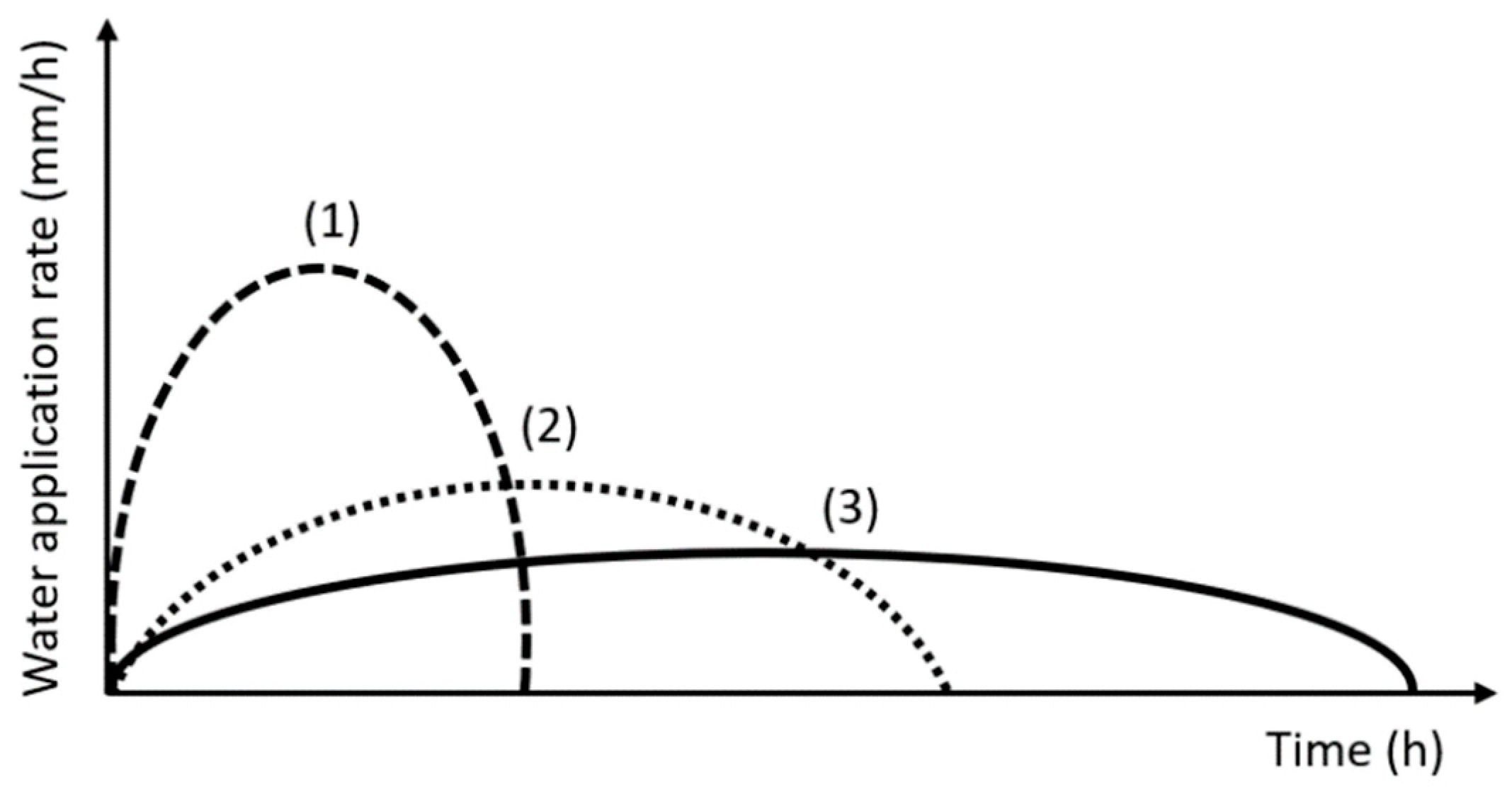
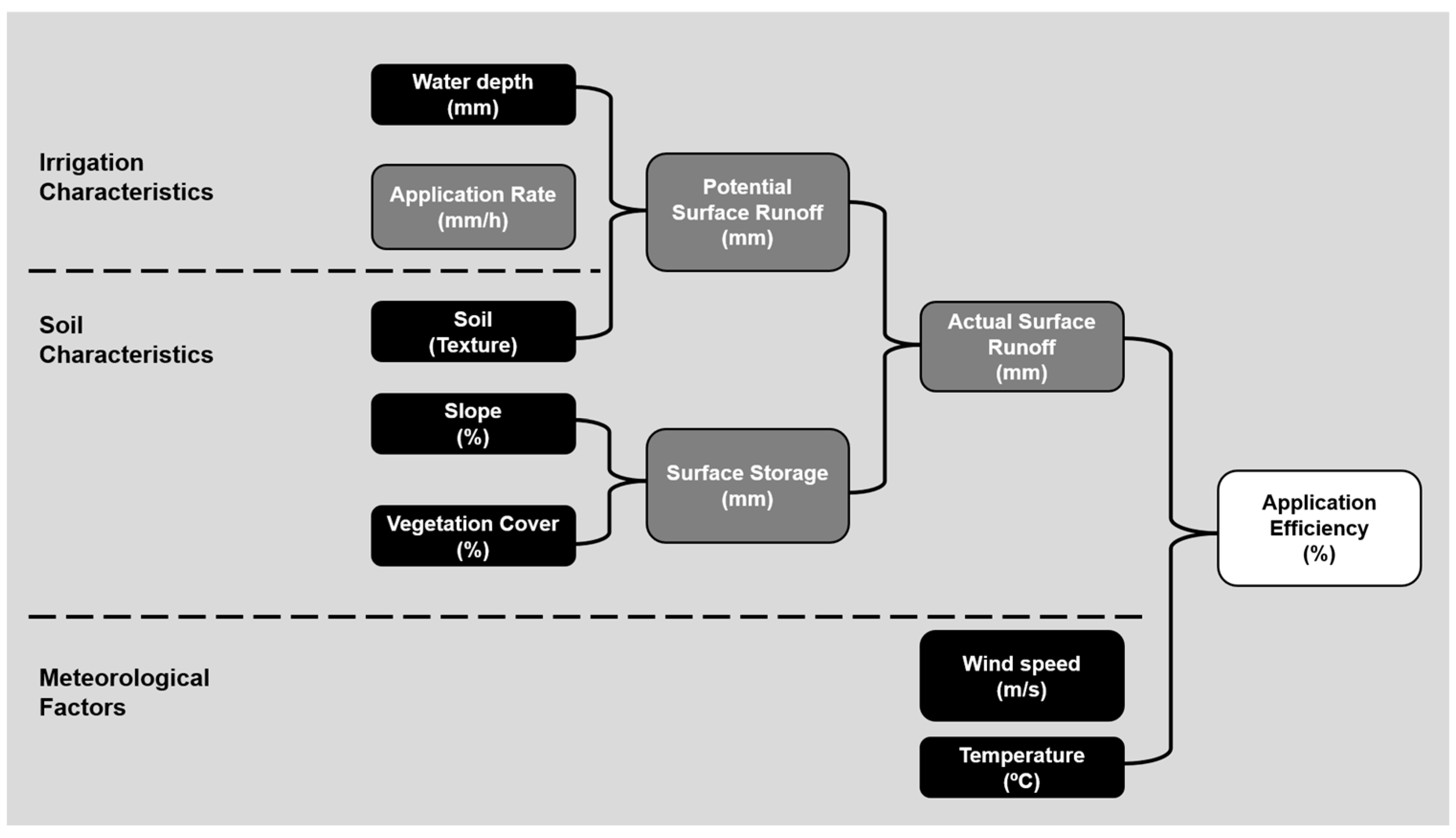
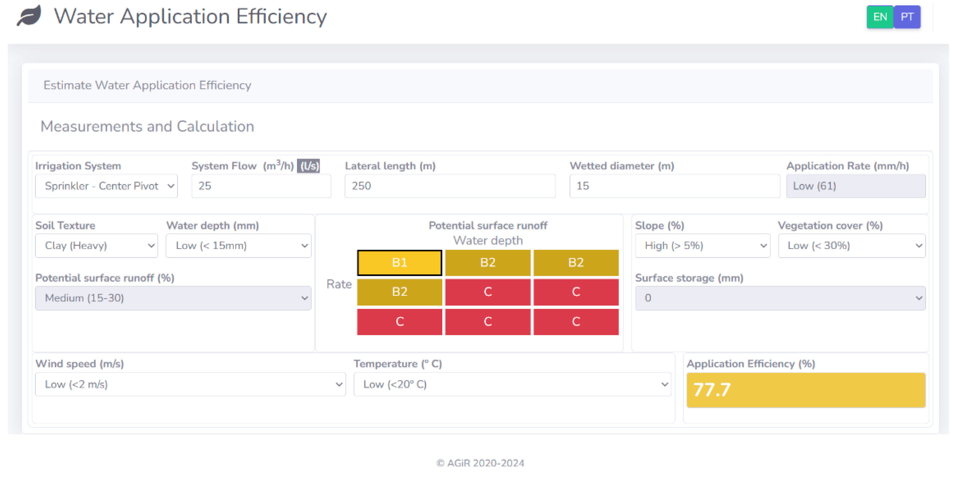
• Step 1: Irrigation system design—flow, length and water diameter inputs to compute the application rate;
• Step 2: Irrigation management—water depth and soil texture inputs;
• First result: Potential runoff (maximum value);
• Step 3: Slope and vegetation cover to estimate surface storage and compute actual runoff;
• Step 4: Climate parameters to estimate water losses;
• Final result: Application efficiency.

One should note that the procedures applied by the computational tool, providing potential runoff and application efficiency results, include adaptations from validated approaches found in the bibliography. Table 4 identifies the main sources of information (data, formulas, classifications, and methods) used to compute the specific variables.

4. Computational Tool Validation and Discussion

Table 5. Data used for the validation of the computational application calculation.

Variables	Case Studies
	C.PIVOT 1	C.PIVOT 2	SOLID SET 1	SOLID SET 2	DRIP 1	DRIP 2
Soil texture	Loam (Medium)	Clay (High)	Loam (Medium)	Loam (Medium)	Loam (Medium)	Loam (Medium)
Peak/Application Rate (mm/h)	60 (Low)	120 (High)	7 (Medium)	3 (Low)	7 (Medium)	4 (Low)
Gross irrigation depth (mm)	7.5 (Low)	15.2 (Medium)	7.2 (Low)	6 (Low)	8.2 (Low)	25.7 (High)
Slope Class (%)	2–5% (Medium)	2–5% (Medium)	2–5% (Medium)	2–5% (Medium)	2–5% (Medium)	2–5% (Medium)
Vegetation Cover (%)	Sunflower (Medium)	Corn (Medium)	Corn (Medium)	Corn (Low)	Corn (Medium)	Melon (Low)
Surface storage (mm)	8	8	8	5	8	5
Wind speed (m/s)	1	>3	0.9	2	–	–
Month of the year and temperature	July (High)	June (Medium)	July (High)	June (Medium)	July (High)	July (High)
Evaporation and wind drift (mm)	1	3	1.1	0.7	0.8 (evaporation)	2.6 (evaporation)

presents data from Pereira [59] for six case studies, two per type of pressure irrigation system, that were simulated to validate the computational application.

Table 6. Results obtained with the computational tool.

Variables	Case Studies
	C.PIVOT 1	C.PIVOT 2	SOLID SET 1	SOLID SET 2	DRIP 1	DRIP 2
PSR classification	A	C	A	A	A	A
Surface runoff (mm)	0	1.3	0	0	0	0
WAE (computational tool) (%)	85 (High)	78 (Medium)	85 (High)	85 (High)	90 (High)	90 (High)
WAE (in the field) (%)	87 (High)	78 (Medium)	83 (High)	88 (High)	- (High)	- (High)

presents the results obtained with the computational application for the application efficiency of the six case studies presented in Table 5.

In all irrigation trials, the water caught varied along laterals by reasonable or good values of uniformity, which contributed to minimizing water losses through surface runoff. Consistently, adverse conditions related to water application depth or wind and distribution, which could result in a low classification level for water application efficiency, were not observed. On the other hand, with the occurrence of very extreme weather events or inadequate water application depths, the field areas will be more prone to overwatering, runoff, or evaporation. It has been found that the irrigation systems, as designed and scheduled, were generally suitable for operating without significant water losses, and deep percolation was not anticipated. It is worth noting that a high WAE, combined with a high DU (characterized by minimal variation in soil water content relative to the scheduled average value), does not guarantee acceptable irrigation performance, as the crop’s water requirements may not be met. On the other hand, a low WAE always means an excess of water loss, and a low DU indicates conditions of water stress and/or ponding areas (negatively affecting crop production). When comparing the six case studies, it is clear that the estimated values for water loss indicated by the PSR are rather small. Only the PIVOT2 and DRIP2 tests showed potential impact. However, only PIVOT2 pointed to propitious conditions for ASR occurrence despite the medium value of surface storage. In all other cases, the WAE achieved a high-class result, which is consistent with model estimates.

5. Conclusions

Full data from the bibliography to the validation process seems to be extremely difficult to find. To our knowledge, the Portuguese report [59], with field data, is the single available publication where we could find some information from (few) irrigation systems (design: flows, application rates, lateral lengths; management; and water depths), soil (texture, AWC, and MAD), topography (slope), crop, and climate (month temperature, wind, and ET), as required to compute Table 5. On the other hand, the basis to obtain parameter values regarding “partial validations” assumed from Table 4 helps to expect reliable results from full validation procedures.

The main innovative feature is the development of a simplified qualitative computational tool, involving several classes of three/four parameters, to estimate the water application efficiency based on adaptation approaches related to several data sources and methodological procedures. The irrigation efficiency values obtained using the computer tool for the six case studies are consistent with the field values presented in Pereira [59]. Thus, it is an easy-to-use support system, pointing to a comprehensive and robust evaluation. Even applying very different information considering the classification of multi-range datasets, the results are consistent with common estimated values of water application efficiencies (pressurized systems) included in manuals, monographs, and papers.

References

1. FAO. The Water-Energy-Food Nexus. A New Approach in Support of Food Security and Sustainable Agriculture; Food and Agriculture Organization of the United Nations: Rome, Italy, 2014; p. 28. [Google Scholar]
2. FAO. Agriculture 4.0—Agricultural Robotics and Automated Equipment for Sustainable Crop Production; Food and Agriculture Organization of the United Nations: Rome, Italy, 2020; p. 25. [Google Scholar]
3. OECD. New Perspectives on the Water-Energy-Food Nexus—Forum Background Note; OECD Headquarters: Paris, France, 2014. [Google Scholar]
4. European Commission: Joint Research Centre; Biedler, M.; Carmona-Moreno, C.; Dondeynaz, C. Position Paper on Water, Energy, Food and Ecosystems (WEFE) Nexus and Sustainable Development Goals (SDGs); Biedler, M., Carmona-Moreno, C., Dondeynaz, C., Eds.; Publications Office, 2019. Available online: https://op.europa.eu/en/publication-detail/-/publication/265bda85-88db-11e9-9369-01aa75ed71a1/language-en (accessed on 11 April 2025).
5. Fatima, N.; Li, Y.; Ahmad, M.; Jabeen, G.; Li, X. Factors Influencing Renewable Energy Generation Development: A Way to Environmental Sustainability. Environ. Sci. Pollut. Res. 2021, 28, 51714–51732. [Google Scholar] [CrossRef] [PubMed]
6. Giordono, L.S.; Flora, J.; Zanocco, C.; Boudet, H. Food Practice Lifestyles: Identification and Implications for Energy Sustainability. Int. J. Environ. Res. Public Health 2022, 19, 5638. [Google Scholar] [CrossRef] [PubMed]
7. Hoff, H. Understanding the Nexus. In Proceedings of the Background Paper for the Bonn2011 Conference: The Water, Energy and Food Security Nexus; Stockholm Environment Institute: Stockholm, Sweden, 2011. [Google Scholar]
8. Lazaro, L.L.B.; Bellezoni, R.A.; Puppim de Oliveira, J.A.; Jacobi, P.R.; Giatti, L.L. Ten Years of Research on the Water-Energy-Food Nexus: An Analysis of Topics Evolution. Front. Water 2022, 4, 859891. [Google Scholar] [CrossRef]
9. Molajou, A.; Afshar, A.; Khosravi, M.; Soleimanian, E.; Vahabzadeh, M.; Variani, H.A. A New Paradigm of Water, Food, and Energy Nexus. Environ. Sci. Pollut. Res. 2023, 30, 107487–107497. [Google Scholar] [CrossRef]
10. Salmoral, G.; Zegarra, E.; Vázquez-Rowe, I.; González, F.; del Castillo, L.; Saravia, G.R.; Graves, A.; Rey, D.; Knox, J.W. Water-Related Challenges in Nexus Governance for Sustainable Development: Insights from the City of Arequipa, Peru. Sci. Total Environ. 2020, 747, 141114. [Google Scholar] [CrossRef]
11. EEA. Climate Change, Impacts and Vulnerability in Europe 2016—An Indicator-Based Report; European Environment Agency: Copenhagen, Denmark, 2017; p. 424. [Google Scholar]
12. FAO. Handbook on Climate Information for Farming Communities—What Farmers Need and What Is Available; Food and Agriculture Organization of the United Nations: Rome, Italy, 2019; p. 184. [Google Scholar]
13. UN. The United Nations World Water Development Report 2021: Valuing Water; UNESCO: Paris, France, 2021. [Google Scholar]
14. La Jeunesse, I.; Cirelli, C.; Aubin, D.; Larrue, C.; Sellami, H.; Afifi, S.; Bellin, A.; Benabdallah, S.; Bird, D.N.; Deidda, R.; et al. Is Climate Change a Threat for Water Uses in the Mediterranean Region? Results from a Survey at Local Scale. Sci. Total Environ. 2016, 543, 981–996. [Google Scholar] [CrossRef]
15. Funk, C.; Raghavan Sathyan, A.; Winker, P.; Breuer, L. Changing Climate—Changing Livelihood: Smallholder’s Perceptions and Adaption Strategies. J. Environ. Manag. 2020, 259, 109702. [Google Scholar] [CrossRef]
16. Zarei, Z.; Karami, E.; Keshavarz, M. Co-Production of Knowledge and Adaptation to Water Scarcity in Developing Countries. J. Environ. Manag. 2020, 262, 110283. [Google Scholar] [CrossRef]
17. EC. Communication from the Commission: The European Green Deal (COM/2019/640); EC: Brussels, Belgium, 2019. [Google Scholar]
18. EC. Summary of CAP Strategic Plans for 2023–2027: Joint Effort and Collective Ambition; European Commission: Brussels, Belgium, 2023; p. 13. [Google Scholar]
19. Van Oost, I. Common Agricultural Policy post-2020. DG AGRI European Commission Unit B2—Research & Innovation; COP: Brussels, Belgium, 2021. [Google Scholar]
20. Communication from the Commission to the European Parliament, the Council, the European Economic and Social Committee and the Committee of the Regions: A Farm to Fork Strategy for a Fair, Healthy and Environmentally-Friendly Food System (COM(2020) 381); European Commission: Brussels, Belgium, 2020.
21. EEA. Circular Economy in Europe—Developing the Knowledge Base; EEA Report; European Environment Agency: Copenhagen, Denmark, 2016. [Google Scholar]
22. EC. Key Policy Objectives of the CAP 2023-27—European Commission. Available online: https://agriculture.ec.europa.eu/common-agricultural-policy/cap-overview/cap-2023-27/key-policy-objectives-cap-2023-27_en (accessed on 30 May 2024).
23. CIHEAM. Dialogues on Mediterranean Water Challenges: Rational Water Use, Water Price versus Value and Lessons Learned from the European Water Framework Directive; SERIES A: Mediterranean Seminars; Centre International de Hautes Etudes Agronomiques Méditerranéennes: Bari, Italy, 2011; p. 196. [Google Scholar]
24. Keller, J.; Bliesner, R.D. Sprinkle and Trickle Irrigation; Reprint of the 1990 edition; Springer: Berlin/Heidelberg, Germany, 2012; ISBN 978-1-4757-1427-2. [Google Scholar]
25. Oliveira, I. Irrigation Techniques-Volumes I & II (In Portuguese), 2nd ed.; Isaurindo Oliveira: Lisboa, Portugal, 2011; ISBN 978-989-20-2692-3. [Google Scholar]
26. Luz, P.B. Guia Para a Avaliação e Seleção de Sistemas de Rega. Programa de Investigação e Formação Pós-Graduada; INIAV: Oeiras, Portugal, 2013. [Google Scholar]
27. OECD. Environmental Indicators for Agriculture: Vol. 1: Concepts and Framework Vol. 2: Issues and Design—“The York Workshop”; Organisation for Economic Co-operation and Development: Paris, Paris, 1999. [Google Scholar]
28. Todorović, N.; Ivković, V.; Kordić, S.; Dimitrieski, V.; Luković, I. IrrigDSS—Decision Support System for Irrigation Scheduling; Faculty of Technical Sciences, University of Novi Sad: Novi Sad, Serbia, 2018. [Google Scholar]
29. Lakhiar, I.A.; Yan, H.; Zhang, C.; Wang, G.; He, B.; Hao, B.; Han, Y.; Wang, B.; Bao, R.; Syed, T.N.; et al. A Review of Precision Irrigation Water-Saving Technology under Changing Climate for Enhancing Water Use Efficiency, Crop Yield, and Environmental Footprints. Agriculture 2024, 14, 1141. [Google Scholar] [CrossRef]
30. Xing, Y.; Wang, X. Precision Agriculture and Water Conservation Strategies for Sustainable Crop Production in Arid Regions. Plants 2024, 13, 3184. [Google Scholar] [CrossRef]
31. Gurmessa, D.K.; Assefa, S.G. A Scoping Review of the Smart Irrigation Literature Using Scientometric Analysis. J. Eng. 2023, 2023, 2537005. [Google Scholar] [CrossRef]
32. Luz, P.B. A Graphical Solution to Estimate Potential Runoff in Center-Pivot Irrigation. Trans. ASABE 2011, 54, 81–92. [Google Scholar] [CrossRef]
33. Ouazaa, S.; Latorre, B.; Burguete, J.; Serreta, A.; Playan, E.; Salvador, R.; Paniagua, P.; Zapata, N. Effect of the Start-Stop Cycle of Center-Pivot Towers on Irrigation Performance: Experiments and Simulations. Agric. Water Manag. 2015, 147, 163–174. [Google Scholar] [CrossRef]
34. Delirhasannia, R.; Sadraddini, A.A.; Nazemi, A.H.; Farsadizadeh, D.; Playan, E. Dynamic Model for Water Application Using Centre Pivot Irrigation. Biosyst. Eng. 2010, 105, 476–485. [Google Scholar] [CrossRef]
35. Al-Agele, H.A.; Mahapatra, D.M.; Prestwich, C.; Higgins, C.W. Dynamic Adjustment of Center Pivot Nozzle Height: An Evaluation of Center Pivot Water Application Pattern and the Coefficient of Uniformity. Appl. Eng. Agric. 2020, 36, 647–656. [Google Scholar] [CrossRef]
36. Luz, P.B.; Heermann, D. A Statistical Approach to Estimating Runoff in Center Pivor Irrigation with Crust Conditions. Agric. Water Manag. 2005, 72, 33–46. [Google Scholar] [CrossRef]
37. Sadeghi, S.H.; Peters, R.T. An Explicit Equation for the Maximum Water Application Depth in Center Pivot Irrigation. J. Irrig. Drain. Eng. 2022, 148, 06022007. [Google Scholar] [CrossRef]
38. Zapata, N.; Bahddou, S.; Latorre, B.; Playan, E. A Simulation Tool to Optimize the Management of Modernized Infrastructures in Collective and On-Farm Irrigation Systems. Agric. Water Manag. 2023, 284, 108337. [Google Scholar] [CrossRef]
39. Barta, R.; Broner, I.; Schneekloth, J.; Waskom, R. Colorado High Plains Irrigation Practices Guide; Special Report No. 14; Colorado Water Resources Research Institute, Colorado State University: Fort Collins, CO, USA, 2004. [Google Scholar]
40. Slattery, K. Determining Irrigation Efficiency and Consumptive Use; GUID 1210-Water Resources Program Guidance; Washington State Department of Ecology: Washington, DC, USA, 2005. [Google Scholar]
41. Rogers, D.H.; Lamm, F.R.; Alam, M.; Trooien, T.P.; Clark, A.; Barnes, P.L. Efficiencies and Water Losses of Irrigation Systems; Irrigation Management Series; Kansas State University: Manhattan, KS, USA, 1997. [Google Scholar]
42. NRCS. National Irrigation Guide. Part 652-Engineering-Handbooks; 210-vi-NEH SC Supplement; USDA National Resources Conservation Service: Columbia, SC, USA, 2016; Chapter 4. [Google Scholar]
43. Martin, D.L.; Kranz, W.; Thompson, A.; Liang, H. Selecting Sprinkler Packages for Center Pivots. Trans. ASABE 2012, 55, 513–523. [Google Scholar] [CrossRef]
44. Lamm, F.R.; Bordovsky, J.P.; Howell, T.A., Sr. A Review of In-Canopy and Near-Canopy Sprinkler Irrigation Concepts. Trans. ASABE 2019, 62, 1355–1364. [Google Scholar] [CrossRef]
45. Skaggs, R.W.; Miller, D.E.; Brooks, R.H. Chapter 4: Soil Water Part I—Properties. In Design and Operation of Farm Irrigation Systems; Jensen, M.E., Ed.; American Society of Agricultural Engineers: Michigan, MI, USA, 1983; ISBN 0-916150-28-3. [Google Scholar]
46. NWA. Inver Grove Heights Stormwater Manual—Appendix E—Curve Number Derivation; Northwest Area: Inver Grove Heights, MN, USA, 2006. [Google Scholar]
47. Kincaid, D. The WEPP Model for Runoff and Erosion Prediction under Sprinkler Irrigation. Trans. ASAE 2002, 45, 67. [Google Scholar] [CrossRef]
48. Kincaid, D.C. Application Rates from Center Pivot Irrigation with Current Sprinkler Types. Appl. Eng. Agric. 2005, 21, 605–610. [Google Scholar] [CrossRef]
49. Gilley, J.R. Suitability of Reduced Pressure Center-Pivots. J. Irrig. Drain. Eng. 1984, 110, 22–34. [Google Scholar] [CrossRef]
50. NRCS. National Irrigation Guide; Part 652. 210-VI-NEH-IG. Nebraska Amendment NE4; NRCS: Washington, DC, USA, 2005. [Google Scholar]
51. Klocke, N.; Kranz, W.; Yonts, C.D.; Wertz, K. Water Runoff from Sprinkler Irrigation: A Case Study; University of Nebraska: Lincoln, RI, USA, 1996. [Google Scholar]
52. Rogers, D.H.; Spurgeon, W.; Sothers, W. Sprinklers Package Effects on Runoff; Irrigation Management Series; Kansas State University: Manhattan, KS, USA, 1994. [Google Scholar]
53. Montgomery, R. Wind Effects on Sprinkler Irrigation Performance; Rain Bird Corporation Technical Paper Library, Irrigation Association: Fairfax, VA, USA, 2013. Available online: https://www.irrigation.org/IA/FileUploads/IA/Resources/TechnicalPapers/2013/WindEffectsOnSprinklerIrrigationPerformance.pdf (accessed on 17 March 2025).
54. Martínez-Cob, A.; Playán, E.; Zapata, N.; Cavero, J.; Medina, E.T.; Puig, M. Contribution of Evapotranspiration Reduction during Sprinkler Irrigation to Application Efficiency. J. Irrig. Drain. Eng. 2008, 134, 745–756. [Google Scholar] [CrossRef]
55. Playan, E.; Garrido, S.; Faci, J.M.; Galán, A. Characterizing Pivot Sprinklers Using an Experimental Irrigation Machine. Agric. Water Manag. 2004, 70, 177–193. [Google Scholar] [CrossRef]
56. Playan, E.; Salvador, R.; Faci, J.M.; Zapata, N.; Martinez-Cob, A.; Sanchez, I. Day and night wind drift and evaporation losses in sprinkler solid-sets and moving laterals. Agric. Water Manag. 2005, 76, 139–159. [Google Scholar] [CrossRef]
57. King, B.A.; Bjorneberg, D.L. Evaluation of potential runoff and erosion of four center pivot irrigation sprinklers. Appl. Eng. Agric. 2011, 27, 75–85. [Google Scholar] [CrossRef]
58. Solomon, K. Irrigation Systems and Water Application Efficiencies; California State University: Fresno, CA, USA, 1988. [Google Scholar]
59. Pereira, L.S. Diagnóstico dos Sistemas de Rega em Pressão. Report—Pediza Project nº 1999.64.006326.1; Departamento de Engenharia Rural, Instituto Superior de Agronomia: Lisboa, Portugal, 2002; 231p. [Google Scholar]
Figure 1. The ten key policy objectives of the Common Agricultural Policy 2023–2027 [22].
Water 17 01217 g001
Figure 2. Theoretical overview of soil profiles with representative canopy cover growth comparing adverse effects of two opposite conditions of Water Application Efficiency (WAE) and Distribution Uniformity (DU): (A) low WAE (60%), high DU (90%), and SE (100%)—larger water losses under deep percolation, evaporation, and wind drift; (B)—high WAE (90%), low DU (60%), and SE (50%)—yield reduction due to water stress.
Water 17 01217 g002
Figure 3. Approximate elliptical patterns of ARs at 3 locations of a center-pivot lateral concerning the correspondent field points: the outer end (1), middle (2), and first third (3). The water application depth is the same at all field points; Pk (1) is twice (2) and three times (3); relatively to Time (1), the time to irrigate a point is double at (2) and triple at (3).
Water 17 01217 g003
Figure 4. Schematic illustration of the WAE calculation.
Water 17 01217 g004
Figure 5. PSR classification.
Water 17 01217 g005
Figure 6. Snapshot of the computational tool for the calculation of the water application efficiency.
Water 17 01217 g006