
Seasonal Patterns of Water Chemistry into Three Boreal Rivers: Implication for Salmonid Incubation and Rearing in the Frame of Hydrological Extremes and Land Use Contexts

 ,
,  , ,
, ,  , and
, and 
Abstract
1. Introduction
2. Materials and Methods
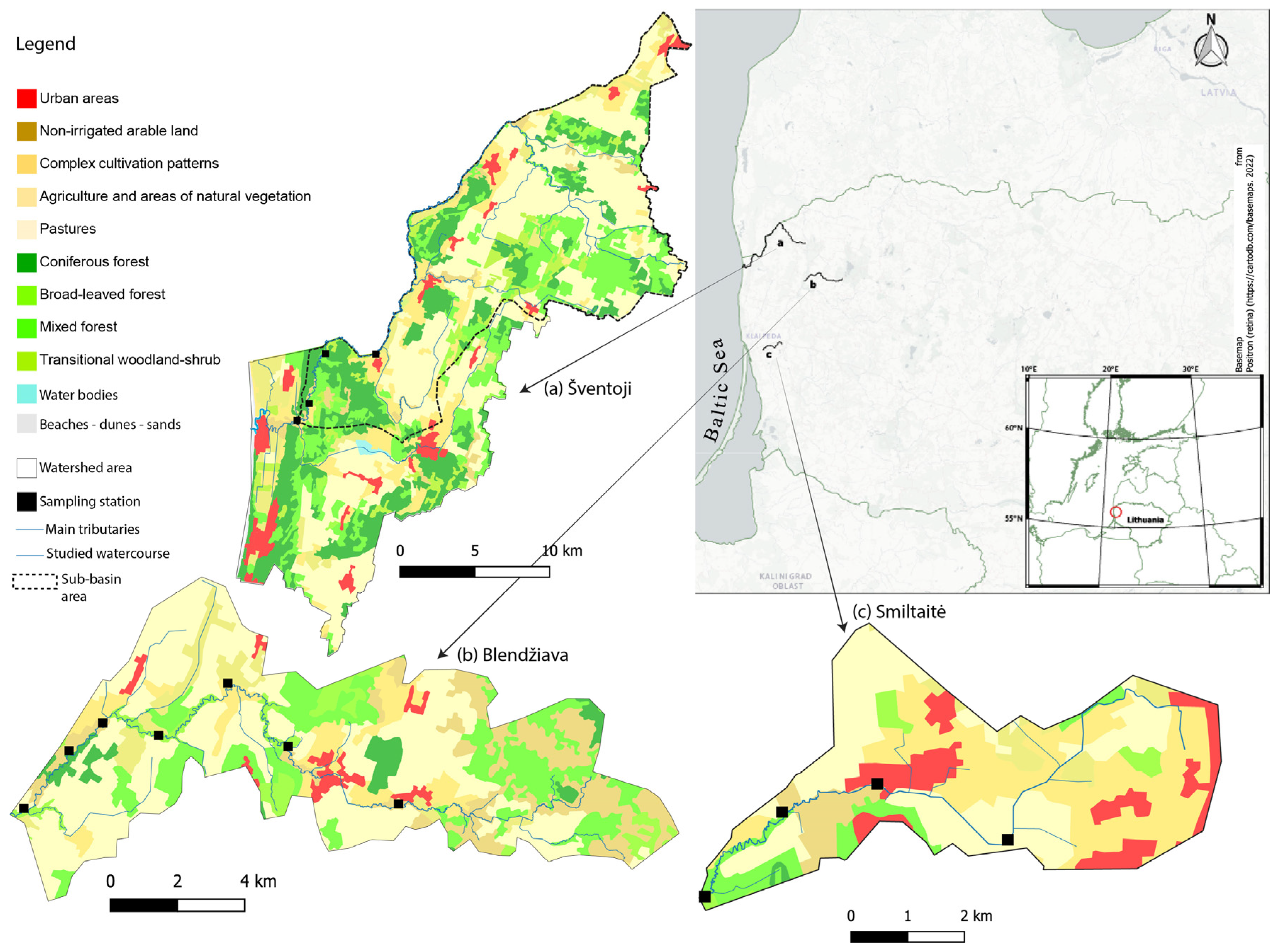
2.1. Study Areas and Land Use
2.2. Sampling Strategy
2.3. Statistical Analyses
3. Results
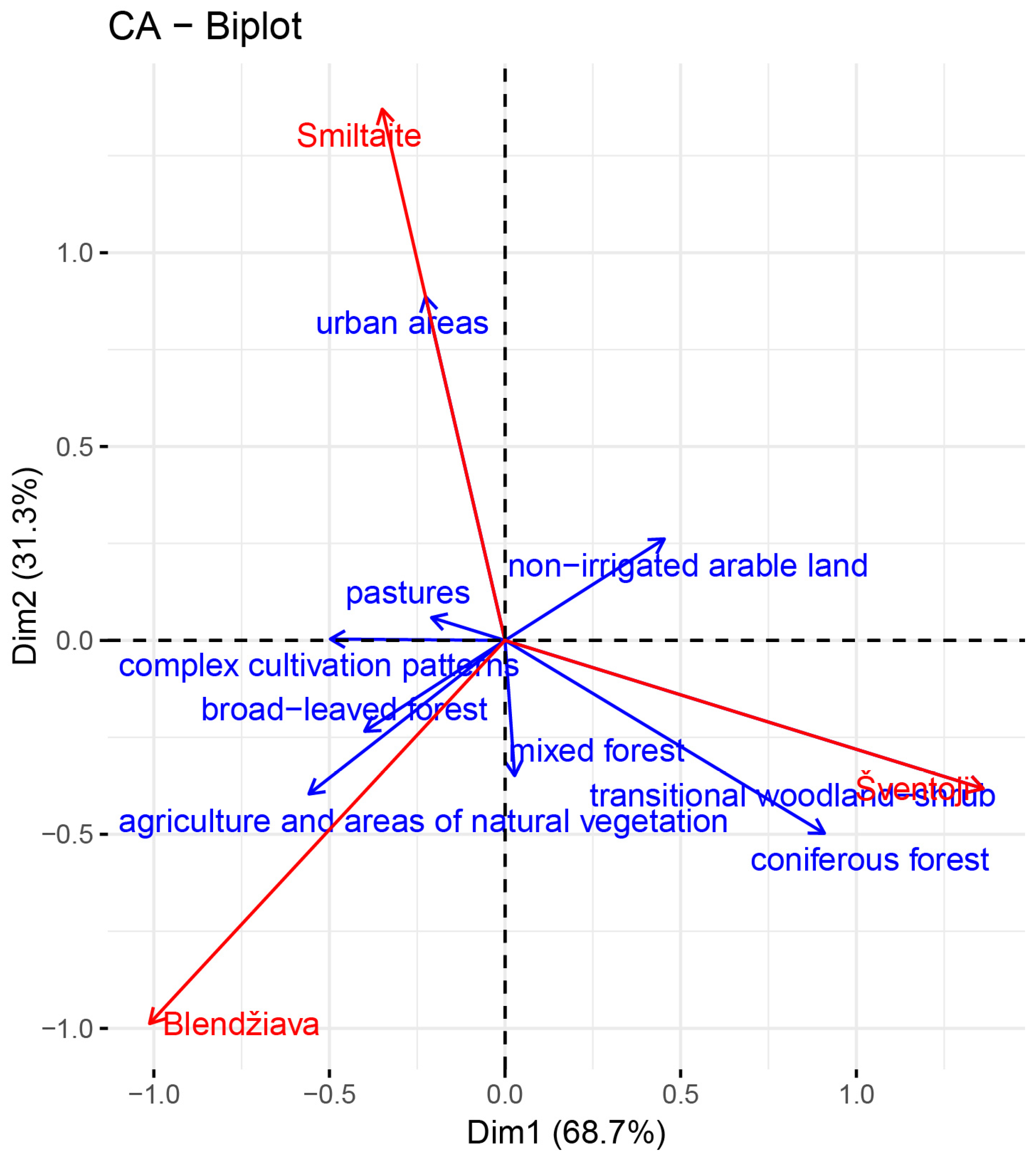
3.1. Land Cover
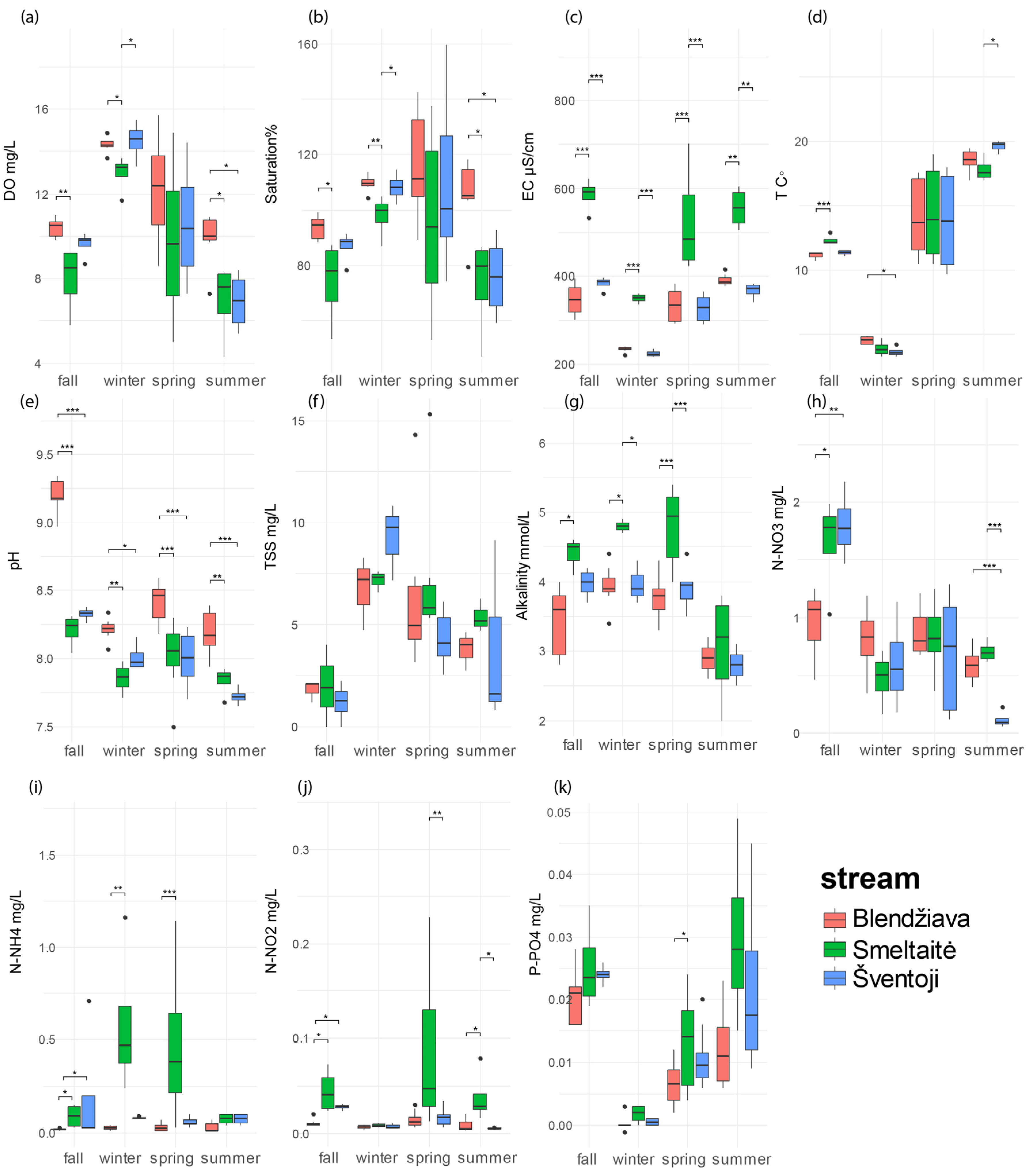
3.2. Seasonal Variations in Water Quality Among Rivers
3.2.1. Fall
3.2.2. Winter
3.2.3. Spring
3.2.4. Summer
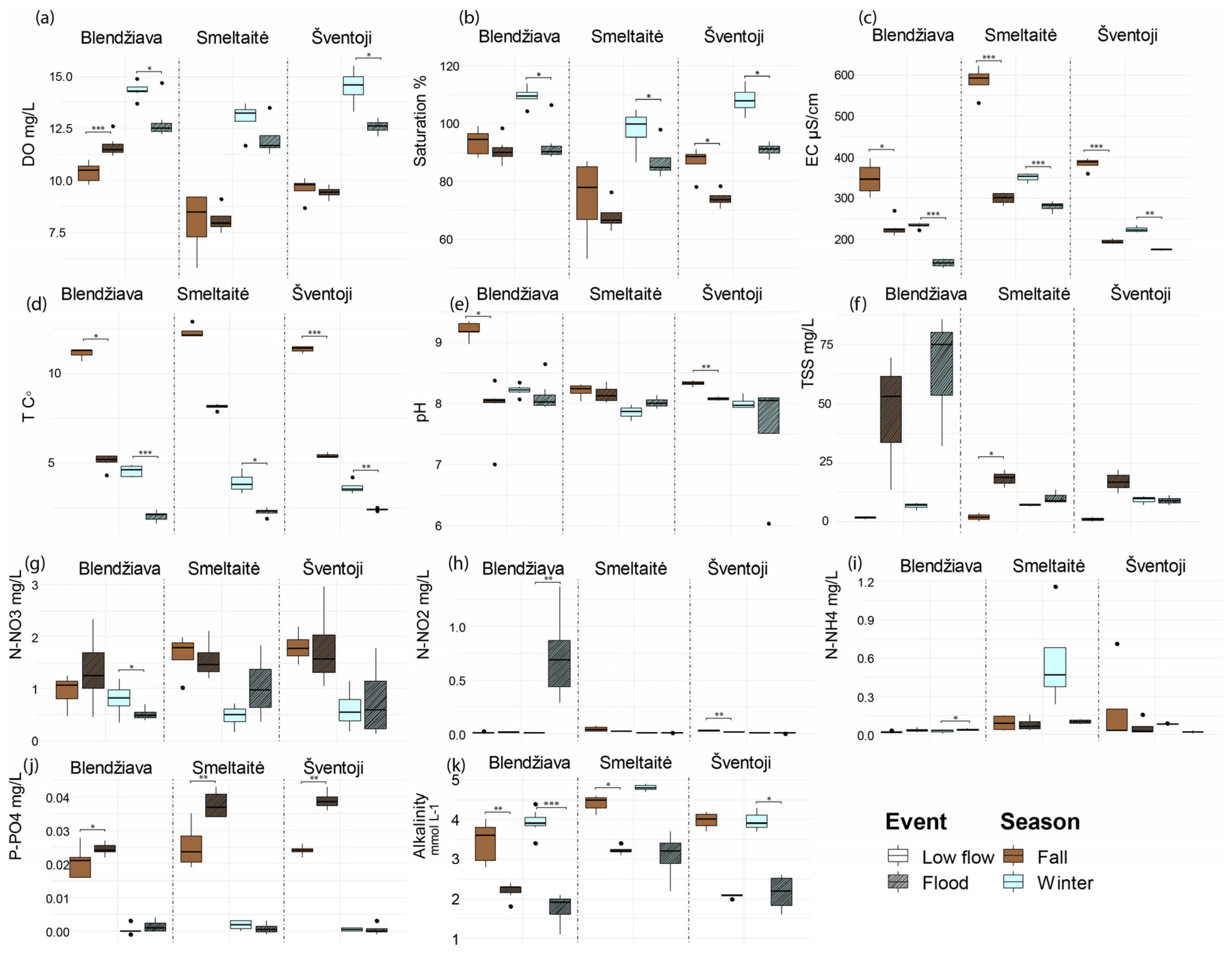
3.3. Rivers’ Behavior Under Extreme Hydrological Events
4. Discussion
4.1. Land Use as the Main Driver of Water Quality
4.2. Accounting for the Seasonality and Hydrological Extremes Shifts
4.3. Implication for Salmonid Incubation and Juvenile Rearing Phases
5. Conclusions
Supplementary Materials
Author Contributions
Funding
Data Availability Statement
Acknowledgments
Conflicts of Interest
References
- Brooks, R.T. Potential impacts of global climate change on the hydrology and ecology of ephemeral freshwater systems of the forests of the northeastern United States. Clim. Chang. 2009, 95, 469–483. [Google Scholar] [CrossRef]
- Nohara, D.; Kitoh, A.; Hosaka, M.; Oki, T. Impact of climate change on river discharge projected by multimodel ensemble. J. Hydrometeorol. 2006, 7, 1076–1089. [Google Scholar] [CrossRef]
- Stanley, E.H.; Fisher, S.G.; Grimm, N.B. Ecosystem expansion and contraction in streams. BioScience 1997, 47, 427–435. [Google Scholar] [CrossRef]
- Dahm, C.N.; Baker, M.A.; Moore, D.I.; Thibault, J.R. Coupled biogeochemical and hydrological responses of streams and rivers to drought. Freshw. Biol. 2003, 48, 1219–1231. [Google Scholar] [CrossRef]
- Sutherland, W.J.; Bailey, M.J.; Bainbridge, I.P.; Brereton, T.; Dick, J.T.; Drewitt, J.; Dulvy, N.K.; Dusic, N.R.; Freckleton, R.P.; Gaston, K.J. Future novel threats and opportunities facing UK biodiversity identified by horizon scanning. J. Appl. Ecol. 2008, 45, 821–833. [Google Scholar] [CrossRef]
- Wilby, R.; Whitehead, P.; Wade, A.; Butterfield, D.; Davis, R.; Watts, G. Integrated modelling of climate change impacts on water resources and quality in a lowland catchment: River Kennet, UK. J. Hydrol. 2006, 330, 204–220. [Google Scholar] [CrossRef]
- Bernal, S.; von Schiller, D.; Sabater, F.; Martí, E. Hydrological extremes modulate nutrient dynamics in mediterranean climate streams across different spatial scales. Hydrobiologia 2013, 719, 31–42. [Google Scholar] [CrossRef]
- Vannote, R.L.; Minshall, G.W.; Cummins, K.W.; Sedell, J.R.; Cushing, C.E. The River Continuum Concept. Can. J. Fish. Aquat. Sci. 1980, 37, 130–137. [Google Scholar] [CrossRef]
- Lange, J.; Haensler, A. Runoff generation following a prolonged dry period. J. Hydrol. 2012, 464, 157–164. [Google Scholar] [CrossRef]
- Larned, S.T.; Datry, T.; Arscott, D.B.; Tockner, K. Emerging concepts in temporary-river ecology. Freshw. Biol. 2010, 55, 717–738. [Google Scholar] [CrossRef]
- Poff, N.L.; Zimmerman, J.K.H. Ecological responses to altered flow regimes: A literature review to inform the science and management of environmental flows. Freshw. Biol. 2010, 55, 194–205. [Google Scholar] [CrossRef]
- Woelfle-Erskine, C.; Larsen, L.G.; Carlson, S.M. Abiotic habitat thresholds for salmonid over-summer survival in intermittent streams. Ecosphere 2017, 8, e01645. [Google Scholar] [CrossRef]
- Hosen, J.D.; Aho, K.S.; Appling, A.P.; Creech, E.C.; Fair, J.H.; Hall, R.O., Jr.; Kyzivat, E.D.; Lowenthal, R.S.; Matt, S.; Morrison, J.; et al. Enhancement of primary production during drought in a temperate watershed is greater in larger rivers than headwater streams. Limnol. Oceanogr. 2019, 64, 1458–1472. [Google Scholar] [CrossRef]
- Burke, N. Physical Controls on Salmon Spawning Habitat Quality and Embryo Fitness: An Integrated Analysis. Ph.D. Thesis, University of Southampton, Southampton, UK, 2011. [Google Scholar]
- Greig, S.; Sear, D.; Carling, P. The impact of fine sediment accumulation on the survival of incubating salmon progeny: Implications for sediment management. Sci. Total Environ. 2005, 344, 241–258. [Google Scholar] [CrossRef] [PubMed]
- Conallin, J. The negative impacts of sedimentation on brown trout (Salmo trutta) natural recruitment, and the management of Danish streams. J. Transdiscipl. Environ. Stud. 2004, 3, 2. [Google Scholar]
- Guarch-Ribot, A.; Butturini, A. Hydrological conditions regulate dissolved organic matter quality in an intermittent headwater stream. From drought to storm analysis. Sci. Total Environ. 2016, 571, 1358–1369. [Google Scholar] [CrossRef]
- Malcolm, I.; Middlemas, C.; Soulsby, C.; Middlemas, S.; Youngson, A. Hyporheic zone processes in a canalised agricultural stream: Implications for salmonid embryo survival. Fundam. Appl. Limnol. 2010, 176, 319. [Google Scholar] [CrossRef]
- Pulg, U.; Barlaup, B.T.; Sternecker, K.; Trepl, L.; Unfer, G. Restoration of spawning habitats of brown trout (Salmo trutta) in a regulated chalk stream. River Res. Appl. 2013, 29, 172–182. [Google Scholar] [CrossRef]
- Calles, O.; Nyberg, L.; Greenberg, L. Temporal and spatial variation in quality of hyporheic water in one unregulated and two regulated boreal rivers. River Res. Appl. 2007, 23, 829–842. [Google Scholar] [CrossRef]
- Dumas, J.; Bassenave, J.; Jarry, M.; Barriere, L.; Glise, S. Effects of fish farm effluents on egg-to-fry development and survival of brown trout in artificial redds. J. Fish Biol. 2007, 70, 1734–1758. [Google Scholar] [CrossRef]
- Adjovu, G.E.; Stephen, H.; Ahmad, S. Spatiotemporal Variability in Total Dissolved Solids and Total Suspended Solids along the Colorado River. Hydrology 2023, 10, 125. [Google Scholar] [CrossRef]
- Soulsby, C.; Malcolm, I.; Youngson, A. Hydrochemistry of the hyporheic zone in salmon spawning gravels: A preliminary assessment in a degraded agricultural stream. Regul. Rivers Res. Manag. Int. J. Devoted River Res. Manag. 2001, 17, 651–665. [Google Scholar] [CrossRef]
- Swietlik, W.; Berry, W.; Gardner, T.; Hill, B.; Jha, M.; Kaufmann, P.; Melzian, B.; Norton, D.; Paul, J.; Rubinstein, N. Developing Water Quality Criteria for Suspended and Bedded Sediments (SABS); Potential Approaches; US EPA Office of Water, Office of Science and Technology, Health and Ecological Criteria Division: Washington, DC, USA, 2003.
- Sutherland, A.B.; Meyer, J.L.; Gardiner, E.P. Effects of land cover on sediment regime and fish assemblage structure in four southern Appalachian streams. Freshw. Biol. 2002, 47, 1791–1805. [Google Scholar] [CrossRef]
- Malcolm, I.; Soulsby, C.; Youngson, A.; Hannah, D.; McLaren, I.; Thorne, A. Hydrological influences on hyporheic water quality: Implications for salmon egg survival. Hydrol. Process. 2004, 18, 1543–1560. [Google Scholar] [CrossRef]
- Sternecker, K.; Wild, R.; Geist, J. Effects of substratum restoration on salmonid habitat quality in a subalpine stream. Environ. Biol. Fishes 2013, 96, 1341–1351. [Google Scholar] [CrossRef]
- Severini, E.; Magri, M.; Soana, E.; Bartoli, M.; Faggioli, M.; Celico, F. Irrigation practices affect relationship between reduced nitrogen fertilizer use and improvement of river and groundwater chemistry. Agric. Water Manag. 2023, 289, 108564. [Google Scholar] [CrossRef]
- Jarvie, H.P.; Jürgens, M.D.; Williams, R.J.; Neal, C.; Davies, J.J.; Barrett, C.; White, J. Role of river bed sediments as sources and sinks of phosphorus across two major eutrophic UK river basins: The Hampshire Avon and Herefordshire Wye. J. Hydrol. 2005, 304, 51–74. [Google Scholar] [CrossRef]
- Brinkman, S.F.; Woodling, J.D.; Vajda, A.M.; Norris, D.O. Chronic toxicity of ammonia to early life stage rainbow trout. Trans. Am. Fish. Soc. 2009, 138, 433–440. [Google Scholar] [CrossRef]
- Rubin, J.F.; Glimsäter, C. Egg-to-fry survival of the sea trout in some streams of Gotland. J. Fish Biol. 1996, 48, 585–606. [Google Scholar]
- Binkley, D.; Brown, T.C. Forest practices as nonpoint sources of pollution in North America 1. JAWRA J. Am. Water Resour. Assoc. 1993, 29, 729–740. [Google Scholar] [CrossRef]
- Chapman, D. Critical review of variables used to define effects of fines in redds of large salmonids. Trans. Am. Fish. Soc. 1988, 117, 1–21. [Google Scholar] [CrossRef]
- Bjornn, T.C.; Reiser, D.W. Habitat requirements of salmonids in streams. Am. Fish. Soc. Spec. Publ. 1991, 19, 138. [Google Scholar]
- Billi, P.; Spalevic, V. Suspended sediment yield in Italian rivers. Catena 2022, 212, 106119. [Google Scholar] [CrossRef]
- Gorgoglione, A.; Gregorio, J.; Rios, A.; Alonso, J.; Chreties, C.; Fossati, M. Influence of land use/land cover on surface-water quality of Santa Lucìa river, Uruguay. Sustainability 2020, 12, 4692. [Google Scholar] [CrossRef]
- Van Esbroeck, C.J.; Macrae, M.L.; Brunke, R.I.; McKague, K. Annual and seasonal phosphorus export in surface runoff and tile drainage from agricultural fields with cold temperate climates. J. Great Lakes Res. 2016, 42, 1271–1280. [Google Scholar] [CrossRef]
- Chen, N.; Hong, H. Nitrogen export by surface runoff from a small agricultural watershed in southeast China: Seasonal pattern and primary mechanism. Biogeochemistry 2011, 106, 311–321. [Google Scholar] [CrossRef]
- Maraseni, T.; Mitchell, C. An assessment of carbon sequestration potential of riparian zone of Condamine Catchment, Queensland, Australia. Land Use Policy 2016, 54, 139–146. [Google Scholar] [CrossRef]
- Opperman, J.J.; Lohse, K.A.; Brooks, C.; Kelly, N.M.; Merenlender, A.M. Influence of land use on fine sediment in salmonid spawning gravels within the Russian River Basin, California. Can. J. Fish. Aquat. Sci. 2005, 62, 2740–2751. [Google Scholar] [CrossRef]
- Olyaei, M.A.; Karamouz, M.; Farmani, R. Framework for assessing flood reliability and resilience of wastewater treatment plants. J. Environ. Eng. 2018, 144, 04018081. [Google Scholar] [CrossRef]
- Zouboulis, A.; Tolkou, A. Effect of Climate Change in Wastewater Treatment Plants: Reviewing the Problems and Solutions. In Managing Water Resources Under Climate Uncertainty: Examples from Asia, Europe, Latin America, and Australia; Shrestha, S., Anal, A.K., Salam, P.A., van der Valk, M., Eds.; Springer International Publishing: Cham, Switzerland, 2015; pp. 197–220. [Google Scholar]
- IPCC. Impacts, Adaptation, and Vulnerability. Contribution of Working Group II to the Fifth Assessment Report of the Intergovernmental Panel on Climate Change; Cambridge University Press: Cambridge, NY, USA, 2014. [Google Scholar]
- Šarauskienė, D.; Akstinas, V.; Kriaučiūnienė, J.; Jakimavičius, D.; Bukantis, A.; Kažys, J.; Povilaitis, A.; Ložys, L.; Kesminas, V.; Virbickas, T. Projection of Lithuanian river runoff, temperature and their extremes under climate change. Hydrol. Res. 2018, 49, 344–362. [Google Scholar] [CrossRef]
- Čerkasova, N.; Mėžinė, J.; Idzelytė, R.; Lesutienė, J.; Ertürk, A.; Umgiesser, G. Exploring variability in climate change projections on the Nemunas River and Curonian Lagoon: Coupled SWAT and SHYFEM modeling approach. Ocean Sci. 2024, 20, 1123–1147. [Google Scholar] [CrossRef]
- Jablonskis, J.; Lasinskas, M. Lithuanian river cadastre (discharges, slopes, capacities). Vilnius Lith. 1962, 3, 640. [Google Scholar]
- Gailiušis, B.; Jablonskis, J.; Kovalenkovienė, M. Lithuanian Rivers: Hydrography and Runoff; Lithuanian Energy Institute: Kaunas, Lithuania, 2001; pp. 1–792. [Google Scholar]
- HELCOM. River Restoration in the Baltic Sea Region: Best Practices and Recommendations for Successful Projects. 2021. Available online: https://retrout.org/2021/08/04/river-restoration-in-the-baltic-sea-region-best-practices-and-recommendations-for-successful-projects/ (accessed on 10 March 2024).
- Nemunas River Basin District; Government of the Republic of Lithuania: Vilnius, Lithuania, 2010.
- List of Water Bodies at Risk; Minister of the Environment of the Republic of Lithuania: Vilnius, Lithuania, 2017. (In Lithuanian)
- Venta River Basin District; Government of the Republic of Lithuania: Vilnius, Lithuania, 2010.
- Kesminas, V. Sea trout and salmon populations and rivers in Lithuania: HELCOM assessment of salmon (Salmo salar) and sea trout (Salmo trutta) populations and habitats in rivers flowing to the Baltic Sea. In Baltic Sea Environment Proceedings; Commission, H., Ed.; Baltic Marine Environment Protection Commission: Helsinki, Finland, 2011. [Google Scholar]
- Jablonskis, J.; Janukėnienė, R. Change of Lithuanian River Runoff; Science: Vilnius, Lithuania, 1978. [Google Scholar]
- Kontautas, A.; Rauckis, U. Some data on sea trout population parameters in Minija River basin. Proc. Klaipėda Univ. 1994, 1, 137–142. [Google Scholar]
- Shi, P.; Zhang, Y.; Li, Z.; Li, P.; Xu, G. Influence of land use and land cover patterns on seasonal water quality at multi-spatial scales. Catena 2017, 151, 182–190. [Google Scholar] [CrossRef]
- Ding, J.; Jiang, Y.; Liu, Q.; Hou, Z.; Liao, J.; Fu, L.; Peng, Q. Influences of the land use pattern on water quality in low-order streams of the Dongjiang River basin, China: A multi-scale analysis. Sci. Total Environ. 2016, 551, 205–216. [Google Scholar] [CrossRef]
- Pinardi, M.; Soana, E.; Severini, E.; Racchetti, E.; Celico, F.; Bartoli, M. Agricultural practices regulate the seasonality of groundwater-river nitrogen exchanges. Agric. Water Manag. 2022, 273, 107904. [Google Scholar] [CrossRef]
- Racchetti, E.; Salmaso, F.; Pinardi, M.; Quadroni, S.; Soana, E.; Sacchi, E.; Severini, E.; Celico, F.; Viaroli, P.; Bartoli, M. Is flood irrigation a potential driver of river-groundwater interactions and diffuse nitrate pollution in agricultural watersheds? Water 2019, 11, 2304. [Google Scholar] [CrossRef]
- Severini, E.; Magri, M.; Soana, E.; Bartoli, M. Unraveling the nexus: Exploring river-groundwater interaction as the primary driver of eutrophication in river ecosystems. J. Hydrol. 2024, 645, 132185. [Google Scholar] [CrossRef]
- Jankowski, K.J.; Houser, J.N.; Scheuerell, M.D.; Smits, A.P. Warmer winters increase the biomass of phytoplankton in a large floodplain river. J. Geophys. Res. Biogeosci. 2021, 126, e2020JG006135. [Google Scholar] [CrossRef]
- Thellman, A.; Jankowski, K.J.; Hayden, B.; Yang, X.; Dolan, W.; Smits, A.P.; O’Sullivan, A.M. The ecology of river ice. J. Geophys. Res. Biogeosci. 2021, 126, e2021JG006275. [Google Scholar] [CrossRef]
- Gran, G. Determination of the equivalence point in potentiometric titrations. Part II. Analyst 1952, 77, 661–671. [Google Scholar] [CrossRef]
- Bendixen, M. A practical guide to the use of correspondence analysis in marketing research. Mark. Res. Line 1996, 1, 16–36. [Google Scholar]
- Nenadic, O.; Greenacre, M. Correspondence analysis in R, with two-and three-dimensional graphics: The ca package. J. Stat. Softw. 2007, 20, 1–13. [Google Scholar]
- Kassambara, A. Practical Guide to Principal Component Methods in R: PCA, M (CA), FAMD, MFA, HCPC, Factoextra. Volume 2. Sthda. 2017. Available online: https://www.sthda.com/english/wiki/practical-guide-to-principal-component-methods-in-r?title=practical-guide-to-principal-component-methods-in-r (accessed on 20 April 2024).
- R Core Team. R: A Language and Environment for Statistical Computing. v 4.4.0. 2023. Available online: https://www.gbif.org/tool/81287/r-a-language-and-environment-for-statistical-computing (accessed on 20 April 2024).
- Kassambara, A. rstatix: Pipe-Friendly Framework for Basic Statistical Tests. v. 0.6.0. 2021. Available online: https://rpkgs.datanovia.com/rstatix/ (accessed on 20 April 2024).
- Kassambara, A. factoextra: Extract and Visualize the Results of Multivariate Data Analyses. R Package Version 1.0.4. 2016. Available online: https://rpkgs.datanovia.com/factoextra/index.html (accessed on 20 April 2024).
- Wickham, H.; Chang, W.; Henry, L.; Pedersen, T.L.; Takahashi, K.; Wilke, C.; Woo, K.; Yutani, H.; Dunnington, D.; van den Brand, T. Package ‘ggplot2’. Create Elegant Data Visualisations Using the Grammar of Graphics. Version 3.5.1. 2016. Available online: https://ggplot2.tidyverse.org/reference/ggplot2-package.html (accessed on 20 April 2024).
- McDowell, R.W.; Hamilton, D.P. Nutrients and eutrophication: Introduction. Mar. Freshw. Res. 2013, 64, iii–vi. [Google Scholar] [CrossRef]
- Wu, T.; Zhu, G.; Zhu, M.; Xu, H.; Zhang, Y.; Qin, B. Use of conductivity to indicate long-term changes in pollution processes in Lake Taihu, a large shallow lake. Environ. Sci. Pollut. Res. 2020, 27, 21376–21385. [Google Scholar] [CrossRef] [PubMed]
- Sager, P.E. Ecological Aspects of Eutrophication. Water Int. 1976, 1, 11–17. [Google Scholar] [CrossRef]
- Sivarajah, B.; Simmatis, B.; Favot, E.J.; Palmer, M.J.; Smol, J.P. Eutrophication and climatic changes lead to unprecedented cyanobacterial blooms in a Canadian sub-Arctic landscape. Harmful Algae 2021, 105, 102036. [Google Scholar] [CrossRef]
- Nika, N. Reproductive Ecology and Success of Sea Trout Salmo trutta L. in a Small Lowland Stream of Western Lithuania. Doctoral Dissertation, Klaipeda University, Coastal Research and Planning Institute, Klaipeda, Lithuania, 2011. [Google Scholar]
- Jeon, I.; Nam, K. Change in the site density and surface acidity of clay minerals by acid or alkali spills and its effect on pH buffering capacity. Sci. Rep. 2019, 9, 9878. [Google Scholar] [CrossRef]
- Kumari, N.; Mohan, C. Basics of Clay Minerals and Their Characteristic Properties; IntechOpen: London, UK, 2021. [Google Scholar]
- Cai, W.-J.; Hu, X.; Huang, W.-J.; Murrell, M.C.; Lehrter, J.C.; Lohrenz, S.E.; Chou, W.-C.; Zhai, W.; Hollibaugh, J.T.; Wang, Y. Acidification of subsurface coastal waters enhanced by eutrophication. Nat. Geosci. 2011, 4, 766–770. [Google Scholar] [CrossRef]
- Sunda, W.G.; Cai, W.-J. Eutrophication induced CO2-acidification of subsurface coastal waters: Interactive effects of temperature, salinity, and atmospheric p CO2. Environ. Sci. Technol. 2012, 46, 10651–10659. [Google Scholar] [CrossRef]
- Sutela, T.; Vehanen, T.; Jounela, P. Response of fish assemblages to water quality in boreal rivers. Hydrobiologia 2010, 641, 1–10. [Google Scholar] [CrossRef]
- Delgado, J.A.; Dillon, M.A.; Sparks, R.T.; Essah, S.Y. A decade of advances in cover crops. J. Soil Water Conserv. 2007, 62, 110A–117A. [Google Scholar]
- Dabney, S.M.; Delgado, J.A.; Meisinger, J.J.; Schomberg, H.H.; Liebig, M.A.; Kaspar, T.; Mitchell, J.; Reeves, W. Using cover crops and cropping systems for nitrogen management. Adv. Nitrogen Manag. Water Qual. 2010, 66, 231–282. [Google Scholar]
- Ross, S.M.; Izaurralde, R.C.; Janzen, H.; Robertson, J.; McGill, W.B. The nitrogen balance of three long-term agroecosystems on a boreal soil in western Canada. Agric. Ecosyst. Environ. 2008, 127, 241–250. [Google Scholar] [CrossRef]
- Heathwaite, A.L.; Johnes, P.J.; Peters, N.E. Trends in nutrients. Hydrol. Process. 1996, 10, 263–293. [Google Scholar] [CrossRef]
- Malcolm, I.A.; Youngson, A.F.; Soulsby, C. Survival of salmonid eggs in a degraded gravel-bed stream: Effects of groundwater–surface water interactions. River Res. Appl. 2003, 19, 303–316. [Google Scholar] [CrossRef]
- Kato, T.; Kuroda, H.; Nakasone, H. Runoff characteristics of nutrients from an agricultural watershed with intensive livestock production. J. Hydrol. 2009, 368, 79–87. [Google Scholar] [CrossRef]
- Yang, Q.; Tian, H.; Li, X.; Ren, W.; Zhang, B.; Zhang, X.; Wolf, J. Spatiotemporal patterns of livestock manure nutrient production in the conterminous United States from 1930 to 2012. Sci. Total Environ. 2016, 541, 1592–1602. [Google Scholar] [CrossRef]
- Finn, R.N. The physiology and toxicology of salmonid eggs and larvae in relation to water quality criteria. Aquat. Toxicol. 2007, 81, 337–354. [Google Scholar] [CrossRef]
- Kincheloe, J.W.; Wedemeyer, G.A.; Koch, D.L. Tolerance of developing salmonid eggs and fry to nitrate exposure. Bull. Environ. Contam. Toxicol. 1979, 23, 575–578. [Google Scholar] [CrossRef]
- Crisp, T. Trout and Salmon: Ecology, Conservation and Rehabilitation; John Wiley & Sons: Hoboken, NJ, USA, 2008. [Google Scholar]
- Greig, S.; Sear, D.; Carling, P. A field-based assessment of oxygen supply to incubating Atlantic salmon (Salmo salar) embryos. Hydrol. Process. Int. J. 2007, 21, 3087–3100. [Google Scholar] [CrossRef]
- Williams, E.; Eddy, F. Effect of nitrite on the embryonic development of Atlantic salmon (Salmo salar). Can. J. Fish. Aquat. Sci. 1989, 46, 1726–1729. [Google Scholar] [CrossRef]
- Smialek, N.; Pander, J.; Geist, J. Environmental threats and conservation implications for Atlantic salmon and brown trout during their critical freshwater phases of spawning, egg development and juvenile emergence. Fish. Manag. Ecol. 2021, 28, 437–467. [Google Scholar] [CrossRef]
- Peterson, R.; Daye, P.; Metcalfe, J. Inhibition of Atlantic salmon (Salmo salar) hatching at low pH. Can. J. Fish. Aquat. Sci. 1980, 37, 770–774. [Google Scholar] [CrossRef]
- Singleton, H. Ambient Water Quality Guidelines (Criteria) for Turbidity, Suspended and Benthic Sediments; British Columbia Ministry of Water, Land and Air Protection: Victoria, BC, Canada, 2001.
- Peña-Guerrero, M.D.; Nauditt, A.; Muñoz-Robles, C.; Ribbe, L.; Meza, F. Drought impacts on water quality and potential implications for agricultural production in the Maipo River Basin, Central Chile. Hydrol. Sci. J. 2020, 65, 1005–1021. [Google Scholar] [CrossRef]
- Vybernaite-Lubiene, I.; Zilius, M.; Saltyte-Vaisiauske, L.; Bartoli, M. Recent trends (2012–2016) of N, Si, and P export from the Nemunas River Watershed: Loads, unbalanced stoichiometry, and threats for downstream aquatic ecosystems. Water 2018, 10, 1178. [Google Scholar] [CrossRef]
- Liu, Y.; Su, B.; Mu, H.; Zhang, Y.; Chen, L.; Wu, B. Effects of point and nonpoint source pollution on urban rivers: From the perspective of pollutant composition and toxicity. J. Hazard. Mater. 2023, 460, 132441. [Google Scholar] [CrossRef]
- Mosley, L.M. Drought impacts on the water quality of freshwater systems; review and integration. Earth-Sci. Rev. 2015, 140, 203–214. [Google Scholar] [CrossRef]
- Povilaitis, A. Phosphorus trends in Lithuanian Rivers affected by agricultural non-point pollution. Environ. Res. Eng. Manag. 2004, 4, 17–27. [Google Scholar]
- Trentman, M.T.; Tank, J.L.; Shepherd, H.A.; Marrs, A.J.; Welsh, J.R.; Goodson, H.V. Characterizing bioavailable phosphorus concentrations in an agricultural stream during hydrologic and streambed disturbances. Biogeochemistry 2021, 154, 509–524. [Google Scholar] [CrossRef]
- Wong, C.H.; Barton, G.W.; Barford, J.P. The nitrogen cycle and its application in wastewater treatment. In The Handbook of Water and Wastewater Microbiology; Mara, D., Horan, N., Eds.; Academic Press: Cambridge, MA, USA, 2003; pp. 427–440. [Google Scholar]
- Zhou, H.; Li, X.; Xu, G.; Yu, H. Overview of strategies for enhanced treatment of municipal/domestic wastewater at low temperature. Sci. Total Environ. 2018, 643, 225–237. [Google Scholar] [CrossRef] [PubMed]
- Bach, H.; Christensen, N.; Kristensen, P. The State of the Environment in Denmark, 2001; NERI Technical Report; Ministry of the Environment: Copenhagen, Denmark, 2002.
- Schepers, J.S.; Vavricka, E.J.; Andersen, D.R.; Wittmuss, H.D.; Schuman, G.E. Agricultural runoff during a drought period. Water Pollut. Control Fed. 1980, 52, 711–719. [Google Scholar]
- Luke, S.H.; Luckai, N.J.; Burke, J.M.; Prepas, E.E. Riparian areas in the Canadian boreal forest and linkages with water quality in streams. Environ. Rev. 2007, 15, 79–97. [Google Scholar] [CrossRef]
- Bauer, A.; Weert, S. Status of nutrient bookkeeping in the Baltic Sea Countries. Rep. Doc. Texte 2015, 95, 2015. [Google Scholar]
- Green, P.A.; Vörösmarty, C.J.; Meybeck, M.; Galloway, J.N.; Peterson, B.J.; Boyer, E.W. Pre-industrial and contemporary fluxes of nitrogen through rivers: A global assessment based on typology. Biogeochemistry 2004, 68, 71–105. [Google Scholar] [CrossRef]
- Lawlor, P.A.; Helmers, M.J.; Baker, J.L.; Melvin, S.W.; Lemke, D.W. Nitrogen application rate effects on corn yield and nitrate-nitrogen concentration and loss in subsurface drainage. In Proceedings of the 2005 ASAE Annual Meeting, Alor Setar, Malaysia, 20–22 August 2005; American Society of Agricultural and Biological Engineers: St. Joseph, MI, USA, 2005. [Google Scholar]
- Szewczyk, C.J.; Smith, E.M.; Benitez-Nelson, C.R. Temperature sensitivity of oxygen demand varies as a function of organic matter source. Front. Mar. Sci. 2023, 10, 1133336. [Google Scholar] [CrossRef]
- White, J.; Khamis, K.; Dugdale, S.; Jackson, F.; Malcolm, I.; Krause, S.; Hannah, D. Drought impacts on river water temperature: A process-based understanding from temperate climates. Hydrol. Process. 2023, 37, e14958. [Google Scholar] [CrossRef]
- Haapala, H.; Sepponen, P.; Meskus, E. Effect of spring floods on water acidity in the Kiiminkijoki area, Finland. Oikos 1975, 26, 26–31. [Google Scholar] [CrossRef]
- Brils, J. Sediment monitoring and the European water framework directive. Ann. Dell’‘istituto Super. Di Sanita 2008, 44, 218. [Google Scholar]
- Nore, A. The Effect of Turbulence on Oxygen Uptake of Water. Master’s Thesis, NTNU, Trondheim, Norway, 2022. [Google Scholar]
- Alderdice, D.; Wickett, W.; Brett, J. Some effects of temporary exposure to low dissolved oxygen levels on Pacific salmon eggs. J. Fish. Board Can. 1958, 15, 229–250. [Google Scholar] [CrossRef]
- Wickett, W.P. The oxygen supply to salmon eggs in spawning beds. J. Fish. Board Can. 1954, 11, 933–953. [Google Scholar] [CrossRef]
- Washington State Department of Ecology. Evaluating Criteria for the Protection of Freshwater Aquatic Life in Washington’s Surface Water Quality Standards: Dissolved Oxygen. 2002; p. 90. Available online: https://apps.ecology.wa.gov/publications/SummaryPages/0010071.html (accessed on 20 April 2024).
- Matthews, K.; Berg, N. Rainbow trout responses to water temperature and dissolved oxygen stress in two southern California stream pools. J. Fish Biol. 1997, 50, 50–67. [Google Scholar] [CrossRef]
- Spoor, W. Distribution of fingerling brook trout, Salvelinus fontinalis (Mitchill), in dissolved oxygen concentration gradients. J. Fish Biol. 1990, 36, 363–373. [Google Scholar] [CrossRef]
- Bams, R. Adaptations of sockeye salmon associated with incubation in stream gravels. In Symposium on Salmon and Trout in Streams; University of British Columbia: Vancouver, BC, Canada, 1969; p. 87. [Google Scholar]
- Claire, E.W.; Phillips, R.W. The stonefly Acroneuria pacifica as a potential predator on salmonid embryos. Trans. Am. Fish. Soc. 1968, 97, 50–52. [Google Scholar] [CrossRef]
- Heywood, M.; Walling, D. The sedimentation of salmonid spawning gravels in the Hampshire Avon catchment, UK: Implications for the dissolved oxygen content of intragravel water and embryo survival. Hydrol. Process. Int. J. 2007, 21, 770–788. [Google Scholar] [CrossRef]
- McDaniels, T.; Wilmot, S.; Healey, M.; Hinch, S. Vulnerability of Fraser River sockeye salmon to climate change: A life cycle perspective using expert judgments. J. Environ. Manag. 2010, 91, 2771–2780. [Google Scholar] [CrossRef]
- Massa, F.; Bagliniere, J.; Prunet, P.; Grimaldi, C. Egg-to-Fry Survival of Brown Trout (Salmo trutta) and Chemical Environment in the Redd. Cybium Int. J. Ichthyol. 2000, 24, 129–140. [Google Scholar]
- Burkhalter, D.E.; Kaya, C.M. Effects of prolonged exposure to ammonia on fertilized eggs and sac fry of rainbow trout (Salmo gairdneri). Trans. Am. Fish. Soc. 1977, 106, 470–475. [Google Scholar] [CrossRef]
- Isaak, D.J.; Young, M.K. Cold-water habitats, climate refugia, and their utility for conserving salmonid fishes. Can. J. Fish. Aquat. Sci. 2023, 80, 1187–1206. [Google Scholar] [CrossRef]
- Crisp, D. Environmental requirements of common riverine European salmonid fish species in fresh water with particular reference to physical and chemical aspects. Hydrobiologia 1996, 323, 201–221. [Google Scholar] [CrossRef]
- Elliott, J. Some aspects of thermal stress on freshwater teleosts. Stress Fish 1981, 1981, 209–245. [Google Scholar]
- Elliott, J.; Hurley, M. A functional model for maximum growth of Atlantic salmon parr, Salmo salar, from two populations in northwest England. Funct. Ecol. 1997, 11, 592–603. [Google Scholar] [CrossRef]
- Davis, J.C. Minimal dissolved oxygen requirements of aquatic life with emphasis on Canadian species: A review. J. Fish. Board Can. 1975, 32, 2295–2332. [Google Scholar] [CrossRef]
- Martin, B.T.; Pike, A.; John, S.N.; Hamda, N.; Roberts, J.; Lindley, S.T.; Danner, E.M. Phenomenological vs. biophysical models of thermal stress in aquatic eggs. Ecol. Lett. 2017, 20, 50–59. [Google Scholar] [CrossRef] [PubMed]
- Geist, D.R.; Hanrahan, T.P.; Arntzen, E.V.; McMichael, G.A.; Murray, C.J.; Chien, Y.-J. Physicochemical characteristics of the hyporheic zone affect redd site selection by chum salmon and fall Chinook salmon in the Columbia River. N. Am. J. Fish. Manag. 2002, 22, 1077–1085. [Google Scholar] [CrossRef]
- Burril, S.E.; Zimmerman, C.E.; Finn, J.E. Characteristics of Fall Chum Salmon Spawning Habitat on a Mainstem River in Interior Alaska. 2010. Available online: https://pubs.usgs.gov/publication/ofr20101164 (accessed on 9 March 2024).
- Stanley, J.G.; Trial, J.G. Habitat Suitability Index Models: Nonmigratory Freshwater Life Stages of Atlantic Salmon; US Department of the Interior, National Biological Service: Washington, DC, USA, 1995; Volume 3.
- McLaughlin, B.C.; Ackerly, D.D.; Klos, P.Z.; Natali, J.; Dawson, T.E.; Thompson, S.E. Hydrologic refugia, plants, and climate change. Glob. Chang. Biol. 2017, 23, 2941–2961. [Google Scholar] [CrossRef]
- Bean, J.R.; Wilcox, A.C.; Woessner, W.W.; Muhlfeld, C.C. Multiscale hydrogeomorphic influences on bull trout (Salvelinus confluentus) spawning habitat. Can. J. Fish. Aquat. Sci. 2015, 72, 514–526. [Google Scholar] [CrossRef]
- Larsen, L.G.; Woelfle-Erskine, C. Groundwater is key to salmonid persistence and recruitment in intermittent Mediterranean-climate streams. Water Resour. Res. 2018, 54, 8909–8930. [Google Scholar] [CrossRef]
- USEPA. 1999 Update of Ambient Water Quality Criteria for Ammonia; USEPA: Washington, DC, USA, 1999.
- EIFAC. Water Quality Criteria for European Freshwater Fish; Report on Ammonia and Inland Fisheries; FAO: Rome, Italy, 1970. [Google Scholar]
- Russo, R.C.; Thurston, R.V. Toxicity of ammonia, nitrite and nitrate to fishes. Aquac. Water Qual. 1991, 3, 58–89. [Google Scholar]
- Eddy, F. Ammonia in estuaries and effects on fish. J. Fish Biol. 2005, 67, 1495–1513. [Google Scholar] [CrossRef]
- Emerson, K.; Russo, R.C.; Lund, R.E.; Thurston, R.V. Aqueous ammonia equilibrium calculations: Effect of pH and temperature. J. Fish. Board Can. 1975, 32, 2379–2383. [Google Scholar] [CrossRef]
- Randall, D.J.; Tsui, T. Ammonia toxicity in fish. Mar. Pollut. Bull. 2002, 45, 17–23. [Google Scholar] [CrossRef] [PubMed]
- Calamari, D.; Marchetti, R.; Vailati, G. Effects of Long-Term Exposure to Ammonia on the Developmental Stages of Rainbow Trout(Salmo gairdneri Richardson). Int. Explor. Mer. 1981, 178, 81–86. [Google Scholar]
- Ip, Y.; Chew, S.; Randall, D. Ammonia toxicity, tolerance, and excretion. Fish Physiol. 2001, 20, 109–148. [Google Scholar]
- Chen, B.; Li, Y. Numerical modeling of biofilm growth at the pore scale. In Proceedings of the 1999 Conference on Hazardous Waste Research, St. Louis, MI, USA, 24–27 May 1999; pp. 215–226. [Google Scholar]
- Battin, T.J.; Kaplan, L.A.; Newbold, J.D.; Cheng, X.; Hansen, C. Effects of current velocity on the nascent architecture of stream microbial biofilms. Appl. Environ. Microbiol. 2003, 69, 5443–5452. [Google Scholar] [CrossRef] [PubMed]
- McKean, J.; Tonina, D. Bed stability in unconfined gravel bed mountain streams: With implications for salmon spawning viability in future climates. J. Geophys. Res. Earth Surf. 2013, 118, 1227–1240. [Google Scholar] [CrossRef]
- Neachell, E. Environmental flows: Saving rivers in the third millennium, by A.H. Arthington. 2012. University of California Press: Berkeley, 424. (ISBN 978-0-520-27369-6) Price: £52.00. River Res. Appl. 2014, 30, 132–133. [Google Scholar] [CrossRef]


| Ecological Status Classes | ||||||||
|---|---|---|---|---|---|---|---|---|
| Watercourse | Annual Average ± sd (Min–Max) | River Type | High | Good | Moderate | Poor | Limits for Salmonid Protection | Parameter |
| Sm | 0.017 ± 0.015 (0–0.049) | 1–2 | <0.050 | 0.05–0.09 | 0.091–0.180 | 0.181–0.400 | NA | P-PO43 mg L−1 |
| Sv | 0.015 ± 0.014 (0–0.045) | |||||||
| Bl | 0.01 ± 0.0092 (0–0.028) | |||||||
| Sm | 0.26 ± 0.31 (0.027–1.16) | 1–2 | <0.10 | 0.10–0.20 | 0.21–0.6 | 0.61–1.50 | 0.017–17 [30,87] *‡ | N-NH4+, mg L−1 |
| Sv | 0.079 ± 0.13 (0.015–0.71) | |||||||
| Bl | 0.03 ± 0.016 (0.009–0.07) | |||||||
| Sm | 1.01 ± 0.52 (0.17–2.11) | 1–2 | <1.30 | 1.3–2.3 | 2.31–4.50 | 4.51–10.00 | 20–34 [88] ‡ | N-NO3−, mg L−1 |
| Sv | 0.92 ± 0.75 (0.06–2.97) | |||||||
| Bl | 0.85 ± 0.39 (0.35–2.34) | |||||||
| Sm | 9.65 ± 2.95 (4.33–14.94) | 1 | >8.50 | 8.50–7.50 | 7.49–6.00 | 5.99–3.00 | 7–9 [89,90] ‡† | O2 mg L−1 |
| Bl | 11.92 ± 1.89 (7.35–15.7) | |||||||
| Sv | 10.59 ± 2.65 (5.38–15.48) | 2 | >7.50 | 7.5–6.5 | 6.49–5.00 | 4.99–2.00 | ||
| Sm | 0.04 ± 0.05 (0.007–0.23) | NA | 14 [21,91] ‡ | N-NO2− mg L−1 | ||||
| Bl | 0.11 ± 0.28 (0.003–1.43) | |||||||
| Sv | 0.01 ± 0.01 (0.004–0.034) | |||||||
| Sm | 10.46 ± 5.71 (1.9–19.1) | NA | 0–11 [89] ‡ 19–20 °C [89,92] † | T °C | ||||
| Bl | 9.94 ± 5.9 (1.6–19.5) | |||||||
| Sv | 10.01 ± 6.21 (2.3–20) | |||||||
| Sm | 8.01 ± 0.2 (7.5–8.35) | NA | >6.7 [93] ‡ | pH | ||||
| Bl | 8.36 ± 0.43 (7–9.34) | |||||||
| Sv | 7.96 ± 0.42 (6.03–8.38) | |||||||
| Sm | 8.27 ± 5.33 (0–22) | NA | <25 increment in clear waters [94] ‡§ | TSS mg L−1 | ||||
| Bl | 19.3 ± 26.4 (1.2–86) | |||||||
| Sv | 6.25 ± 5.1 (0–22) | |||||||
Disclaimer/Publisher’s Note: The statements, opinions and data contained in all publications are solely those of the individual author(s) and contributor(s) and not of MDPI and/or the editor(s). MDPI and/or the editor(s) disclaim responsibility for any injury to people or property resulting from any ideas, methods, instructions or products referred to in the content. |
© 2024 by the authors. Licensee MDPI, Basel, Switzerland. This article is an open access article distributed under the terms and conditions of the Creative Commons Attribution (CC BY) license (https://creativecommons.org/licenses/by/4.0/).
Share and Cite
Benetti, R.; Severini, E.; Nika, N.; Čerkasova, N.; Magri, M.; Bartoli, M. Seasonal Patterns of Water Chemistry into Three Boreal Rivers: Implication for Salmonid Incubation and Rearing in the Frame of Hydrological Extremes and Land Use Contexts. Water 2024, 16, 3352. https://doi.org/10.3390/w16233352
Benetti R, Severini E, Nika N, Čerkasova N, Magri M, Bartoli M. Seasonal Patterns of Water Chemistry into Three Boreal Rivers: Implication for Salmonid Incubation and Rearing in the Frame of Hydrological Extremes and Land Use Contexts. Water. 2024; 16(23):3352. https://doi.org/10.3390/w16233352
Chicago/Turabian StyleBenetti, Rudy, Edoardo Severini, Nerijus Nika, Natalja Čerkasova, Monia Magri, and Marco Bartoli. 2024. "Seasonal Patterns of Water Chemistry into Three Boreal Rivers: Implication for Salmonid Incubation and Rearing in the Frame of Hydrological Extremes and Land Use Contexts" Water 16, no. 23: 3352. https://doi.org/10.3390/w16233352
APA StyleBenetti, R., Severini, E., Nika, N., Čerkasova, N., Magri, M., & Bartoli, M. (2024). Seasonal Patterns of Water Chemistry into Three Boreal Rivers: Implication for Salmonid Incubation and Rearing in the Frame of Hydrological Extremes and Land Use Contexts. Water, 16(23), 3352. https://doi.org/10.3390/w16233352