Article

Evaluating Hydrologic Model Performance for Characterizing Streamflow Drought in the Conterminous United States

by
Caelan Simeone
1,*,
Sydney Foks
2,
Erin Towler
3,
Timothy Hodson
4 and
Thomas Over
5
1
Oregon Water Science Center, U.S. Geological Survey, Portland, OR 97204, USA
2
Water Resources Mission Area, U.S. Geological Survey, Tacoma, WA 98402, USA
3
National Center for Atmospheric Research, Boulder, CO 80307, USA
4
Water Resources Mission Area, U.S. Geological Survey, Urbana, IL 61801, USA
5
Central Midwest Water Science Center, U.S. Geological Survey, Urbana, IL 61801, USA
*
Author to whom correspondence should be addressed.
Water 2024, 16(20), 2996; https://doi.org/10.3390/w16202996
Submission received: 13 August 2024 / Revised: 19 September 2024 / Accepted: 29 September 2024 / Published: 21 October 2024

Abstract

:
Hydrologic models are the primary tools that are used to simulate streamflow drought and assess impacts. However, there is little consensus about how to evaluate the performance of these models, especially as hydrologic modeling moves toward larger spatial domains. This paper presents a comprehensive multi-objective approach to systematically evaluating the critical features in streamflow drought simulations performed by two widely used hydrological models. The evaluation approach captures how well a model classifies observed periods of drought and non-drought, quantifies error components during periods of drought, and assesses the models’ simulations of drought severity, duration, and intensity. We apply this approach at 4662 U.S. Geological Survey streamflow gages covering a wide range of hydrologic conditions across the conterminous U.S. from 1985 to 2016 to evaluate streamflow drought using two national-scale hydrologic models: the National Water Model (NWM) and the National Hydrologic Model (NHM); therefore, a benchmark against which to evaluate additional models is provided. Using this approach, we find that generally the NWM better simulates the timing of flows during drought, while the NHM better simulates the magnitude of flows during drought. Both models performed better in wetter eastern regions than in drier western regions. Finally, each model showed increased error when simulating the most severe drought events.

1. Introduction

Drought is a costly natural disaster, sometimes causing billions of dollars’ worth of damage, and has wide-ranging impacts, from agriculture to public health [1,2,3]. While drought has received much attention in the hydrologic literature [4], drought is a complex phenomenon that is difficult to simulate [5,6,7,8,9]. Droughts are commonly separated into four categories: meteorological, agricultural (or soil moisture), hydrological, and socioeconomic [10,11,12]. Meteorological, agricultural, and hydrological droughts occur in physical systems, whereas socioeconomic droughts are the social and economic impacts of drought [12,13]. We focus on streamflow drought, which is a subset of hydrological drought, that Van Loon [11] defines as follows: “a lack of water in the hydrologic system manifesting itself in abnormally low streamflow in rivers.” Streamflow drought can be costly and negatively impact many sectors that rely on streamflow quantity, quality, and timing, such as ecosystem, agricultural, navigation, and municipal services [1].
Due to the importance of streamflow drought, there have been ongoing efforts to simulate and predict drought occurrence and severity [8,14,15,16,17,18,19]. Many studies and models have shown skill in simulating certain drought events; however, there are many different types of drought indicators [11,20,21], and the methodologies used to evaluate models are inconsistent [22]. Differences in the methodologies used to evaluate drought simulations can make model intercomparison difficult, as is the case more broadly in hydrology [23,24].
Streamflow drought is different to normal low flows. Although droughts may include periods of low streamflows, a recurring seasonal low-flow event is not necessarily a drought [25]. Numerous studies have aimed to quantify low flows (e.g., 7-day mean low-flow (Q7) [25]) and evaluate how well models simulate low-flow metrics [26,27,28,29,30], but these metrics alone are inadequate for evaluating model simulations of drought as they do not address the differences between low flows and drought, and often target a specific low-flow magnitude like Q7 instead of evaluating the full period of a drought.
Common model evaluation metrics, like the Nash–Sutcliffe efficiency (NSE; [31]), are often more sensitive to high flows than low flows, making them a poor indicator of predictive accuracy for drought [32]. To address this issue, drought studies sometimes use evaluation metrics on standardized drought indices (e.g., standardized streamflow index) or streamflow percentiles [11] instead of directly on the streamflow [6,33,34]. This offers some improvement, but often still focuses a large percentage of the evaluation on non-drought periods. Streamflow droughts are, by definition, abnormal events (often between the 2nd and 30th percentile [35,36]), meaning that, generally, 70–98% of streamflow data represent non-drought conditions. Applying metrics across non-drought periods may inflate or deflate model performance metrics, making them less indicative of a model’s performance when simulating drought [32].
Studies also use different methods of identifying drought events, making model intercomparison and benchmarking difficult. For example, drought can be identified with a fixed method (where a river is in a drought when it drops below a single fixed long-term level) or a variable method (where the drought threshold varies seasonally based on how much water is typically available in that season) [7,18,35,37].
Previous efforts to evaluate the simulation of streamflow drought vary substantially (e.g., using different temporal resolutions, periods or seasons of interest, methods for drought characterization, and different methods for evaluation), which makes model evaluation intercomparisons challenging. One reason for this is that the focus of traditional hydrologic modeling has been on local or regional catchment scales [23], where evaluations typically vary study by study, depending on the application or location. Similarly, studies sometimes focus on a particular drought event (e.g., [33,34,38]), which by design is not conducive to model evaluation intercomparisons. However, as hydrologic modeling moves to encompass national and larger spatial scales, and toward longer (multi-year) runs, there is a need to provide systematic, comprehensive, comparable metrics to evaluate the streamflow drought modeled across hydroclimatic regions. Previous model intercomparison studies have provided systematic evaluation approaches for Earth system models [39] and long-term streamflow performance [24], but Towler et al. [24] only looked at one low-flow metric.
Given the shift toward standardized approaches to the construction and evaluation of national-scale hydrologic models and the importance of streamflow drought, we propose a systematic and comprehensive approach to evaluating simulations of streamflow drought. We demonstrate the approach through an assessment of the streamflow drought simulation performance of two large-scale hydrological modeling applications in the conterminous United States (CONUS): the National Water Model version 2.1 application of WRF-Hydro (NWM; [40]; accessed through NOAA’s Office of Water Prediction) and the National Hydrologic Model application of the Precipitation-Runoff Modeling System version 1.0 three-step calibration with routing (NHM; [41,42,43]).
Specifically, we use three categories of metrics to evaluate model simulations of streamflow drought:
  • Classification: How well the models simulate the occurrence of observed drought vs. non-drought periods [44] according to Cohen’s kappa [45]. Evaluating model simulation of drought occurrence is one of the simplest but most important measures of model performance in drought simulation.
  • Error Components: How well the models simulate the timing, magnitude, and variability of streamflow during periods of drought according to Spearman’s r [46], percent bias, and the ratio of standard deviations, respectively. This approach examines how errors in streamflow are split across these three components [47].
  • Drought Signatures: How well the models simulate drought duration, intensity, and severity according to the normalized mean absolute errors of annualized data. These three drought characteristics are widely used by the research community and play a large role in the impact of droughts.
This suite of metrics captures many facets of streamflow drought simulation and evaluates them across many hydrologic environments. This approach extends existing model evaluations of drought (e.g., [48]), with additional focus on multi-objective evaluation that emphasizes the critical features of streamflow drought which are relevant to understanding error. The evaluation of these models across a wider number and density of gages provides a more robust understanding of models [49] and importantly captures the heterogeneity in drought responses, which, especially in mountainous regions, can have major implications for regional responses and water security [50]. Applying this comprehensive evaluation in a benchmarking framework for the intercomparison of the NWM and NHM modeling application allows for an improved understanding of the differences and potential limitations and benefits of each model [24]. We apply advances from large sample intercomparison studies [24,49,51] to continue to build on studies examining streamflow drought simulations (e.g., [48]).

2. Materials and Methods

Prior to evaluating streamflow drought using the three categories of metrics, we acquired data at stream gages with sufficient historical records, identified stream gages in regions with similar hydroclimatic characteristics, and identified periods of streamflow drought that were suitable for the demonstration of the drought evaluation framework.

2.1. Modeling Applications and Observed Data

2.1.1. Modeling Applications

The NHM and NWM are similar in their temporal and spatial extent (CONUS-wide), in which the hydrologic state and flux variables are simulated, and in their use in hydrologic estimation and research. However, these modeling applications have some key differences, including the spatial and temporal resolution, parameter estimation techniques, parameter datasets, calibrations, and forcings. The NHM is forced with the 1 km Daymet version 3 product [52], whereas the NWM is forced with the NOAA-produced 1 km Analysis of Record for Calibration version 1.0 forcing dataset [53]. The NWM calculates states and fluxes on a 1 km grid, while the NHM uses hydrological response units and a stream network as the primary geospatial structure [24]. The NWM runs on an hourly timestep, while the NHM is daily.
While the model calibration details can be found in [24,43], here we highlight several key aspects of calibration for each model. The NWM calibrates its parameters for hourly streamflow at 1378 observation stations, mostly in natural (unimpaired) basins. The calibration uses a modified Nash–Sutcliffe efficiency (NSE; [31,54]), which includes the standard NSE, as well as a log-transformed NSE. Then, the NWM employs hydrologic similarity to regionalize the parameters for the remaining watersheds. On the other hand, the NHM considers multiple objectives in a stepwise manner in its calibration routine. First, it balances the water budgets in each hydrologic response unit (HRU), considers the streamflow timing based on a statistically generated dataset, and finally calibrates to the observed streamflow at 1417 gage locations.
Both the NWM and the NHM have been evaluated for their performance in simulating streamflow (e.g., [24,27,55,56,57,58]), but have not yet been evaluated against other models for simulating streamflow drought; they thus serve as good candidates for our methodology. We used daily mean streamflow simulations direct from the NHM and averaged the hourly streamflow simulations from the NWM into a daily mean streamflow for each gage of interest. A daily timestep was chosen for comparison to preserve as much of the event timing relationship as possible while still accommodating common modeling application timescales (many model applications simulate results at a daily timestep). Further descriptions of these modeling applications and calibration techniques are explained in Towler et al. [24] and Hay et al. [43].

2.1.2. Observed Data

The drought performance of both model applications was evaluated at 4662 U.S. Geological Survey (USGS) stream gages across CONUS. We subset the stream gage dataset for benchmarking the hydrologic modeling applications described in Foks et al. [59] to include gages with at least 16 years of daily observations of flow (a longer record was needed to obtain sufficient data during drought periods). The study period spans the climate years (CYs, April 1–March 31) 1985–2016, which is the overlap between the NWM and the NHM historical simulations. Climate years more consistently contain the entire annual low-flow period than calendar years (January through December) or water years (October through September; [60,61]) in CONUS.

2.1.3. Evaluating Regional Performance

We categorized the stream gages into 12 hydrologic regions (Figure 1), defined by their correlation in monthly flows among the minimally altered gages in the Hydro-Climatic Data Network (HCDN; [62]), following approaches by McCabe and Wolock [63]. We then evaluated the regional differences in model performance when simulating streamflow drought by examining the model performance across all stream gages in each region. These same regions were used in the regional drought analysis by Hammond et al. [35]. We attributed stream gages not within the HCDN to the region of the nearest HCDN gage.

2.2. Identification of Drought

We characterized drought using fixed and variable streamflow percentiles and thresholds at the 5th, 10th, 20th, and 30th percentiles, as implemented by Hammond et al. [35]. We converted the daily streamflow observations and model simulations to percentiles for all gages. Within observations or a single model, percentiles allow for the fair classification of drought across different hydroclimatic regions. Percentiles allow for more direct comparisons of low-flow anomalies (i.e., drought) between observations and models without the influence of model bias, which we evaluate elsewhere. The streamflow percentiles were computed with the Weibull plotting position (r/(n + 1), where r is rank and n is the number of data (e.g., [64])). Two types of percentile-based threshold approaches were used: (1) fixed—all modeled or observed flows in the period on record are used to calculate one fixed threshold, and (2) variable—unique thresholds are calculated for each day of the year using only the values for that day from all years on record (Figure S1a,b). We implemented a modified version [65] of the combined threshold level and continuous dry period methods developed by Van Huijgevoort et al. [66] to handle the zero-flow measurements (<0.00028 cubic meters per second; <0.01 cubic feet per second). This method breaks ties between zero-flow days for percentile rankings based on the number of preceding zero-flow days, with days with more preceding zero-flow days receiving lower percentile rankings. Droughts were classified according to whether the streamflow was below the 5th, 10th, 20th, or 30th percentiles (Figure S1c), which roughly correspond to the extreme, severe, moderate, or abnormal drought classifications used by the U.S. Drought Monitor (https://droughtmonitor.unl.edu/, accessed 1 November 2023). This created a time series of drought presence and absence for each stream gage, threshold, and simulated and observed streamflow dataset. For each climate year, we calculated the following:
  • Drought duration: the total number of days below the threshold (days);
  • Drought severity: the sum of flow departures or deficit below the threshold (cms-days);
  • Drought intensity: the maximum drought intensity (minimum percentiles).

2.3. Evaluation for Drought Performance

We evaluate the performance of model simulations of drought by examining the goodness of the match [44] between modeled and observed events (i.e., event classification) and the quality of the simulation for matched events [44]. To evaluate the quality of the simulations during drought, we examine the error components during drought events (Spearman’s r, ratio of standard deviations, and percent bias) and the errors in the important characteristics of drought (drought signatures of duration, severity, and intensity) aggregated to the climate year level. Table 1 shows the streamflow drought statistical metrics included in our systematic evaluation. We evaluated performance in three categories— “Event Classification”, “Error Components”, and “Drought Signatures”—which are described in the subsections below.

2.3.1. Event Classification Evaluation

Drought and non-drought periods were first classified for modeled and observed time series data. Evaluating if the model can correctly classify drought is one of the simplest but most important measures of model performance in drought simulation. If a model cannot correctly simulate when a drought is occurring, the quality of the rest of its predictions in the context of drought may not be particularly useful. We used Cohen’s kappa to evaluate how well the simulated drought periods capture observed drought periods considering each day independently. Cohen’s kappa measures the accuracy of the model classification and accounts for class imbalance in cases where categorical results are not evenly balanced (i.e., for the 20th percentile drought threshold, 80% of days will be non-drought). Cohen’s kappa compares the relative observed agreement (true positives and true negatives from a contingency table or confusion matrix) to the expected agreement. Landis and Koch [67] provide guidelines for interpreting Cohen’s kappa. They describe values < 0 as indicating no agreement and 0–0.20 as slight, 0.21–0.40 as fair, 0.41–0.60 as moderate, 0.61–0.80 as substantial, and 0.81–1 as almost perfect agreement [67]. Cohen’s kappa was calculated as follows:
k = p o p e 1 p e
where p o is the relative observed agreement and p e is the expected agreement or probability of agreement.

2.3.2. Error Components Evaluation

Commonly used metrics of efficiency like NSE are aggregations of model error components, but more information and insights can often be obtained when these error components are decomposed [47,68,69]. Gupta et al. [47] decomposed NSE and showed that “NSE consists of three distinctive components representing the correlation, the bias, and a measure of relative variability in the simulated and observed value.” We evaluated these three individual components of model error rather than a single aggregated metric in order to provide insight into what might be driving model error during periods of drought. To evaluate the model performance during drought periods, we calculated the correlation (which shows errors from timing), bias (which shows errors in the magnitude of the streamflow distribution), and ratio of standard deviations (which evaluates errors in the variability of the streamflow distribution) of the simulated flows corresponding to the observed droughts. We followed a similar approach to that used by Pushpalatha et al. [32] (10th percentile of flow) and Pfannerstill et al. [30] (5th and 20th percentiles of flow) for evaluating the model performance for low flows and calculated our metrics only on values corresponding to drought events.
To evaluate the models’ ability to reproduce the sequence of the observed time series, in other words, the timing of streamflow, during drought periods, we calculated Spearman’s rank correlation coefficient [70,71]. Being based on the ranks of the flow magnitudes, Spearman’s r depends only on the monotonicity of the relation between the observed and simulated flows. As a result, Spearman’s r is a better estimator of the timing correlation than the more common Pearson estimator for streamflow data [72], since it is resistant to nonlinearity and skewness. Spearman’s r is often used to assess flow timing to determine how well a model reproduces the relative position in time of flow values [24,73]. Our calculations began in the same way as those for standard Spearman’s r, where the observed and modeled streamflow are each ranked by magnitude across the entire study period. After calculating ranks, however, we subset the data into periods with observed droughts at the various threshold levels of interest; for example, we took the lowest 20% of flow values for the 20th percentile drought threshold. Spearman’s r is calculated on these subsets as follows:
Spearman’s r = c o v R o b s Q o b s d r o u g h t ,   R s i m Q o b s d r o u g h t s i g m a R o b s Q o b s d r o u g h t s i g m a R s i m Q o b s d r o u g h t
where R(obsQ) and R(simQ) are the ranks of observed and modeled discharges, which are then subset into periods of observed drought. When the streamflow was at zero, we used the continuous dry period method, as described in Section 2.2, to break ties for ranking.
To investigate whether the model over or underestimated the total streamflow volume during drought periods, we calculated the percent bias of the observed flows below the drought threshold versus the modeled flows below the drought threshold ([24]; note that these are thresholds of the equal streamflow percentile, not of the streamflow volume). Our implementation of percent bias for drought flows focused only on flows below a threshold, like the implementation in Yilmaz et al. [74], although they used a 30th percentile threshold while we address a range of thresholds. Percent bias is calculated as follows:
P B i a s = 100   m e a n s i m Q s i m d r o u g h t m e a n o b s Q o b s d r o u g h t m e a n o b s Q o b s d r o u g h t
To provide a first-order estimate of errors in the statistical distribution of simulated flow magnitudes during periods of drought, we calculated the ratio of standard deviations between the modeled and observed streamflow (rSD) [24],
rSD = σ s i m d r o u g h t σ o b s d r o u g h t
This metric shows the relative variability between simulation and observations [24,47,75] and indicates if the model has over- or under-simulated the variability during periods of drought. The combination of rSD and percent bias evaluates whether the distribution of the simulated drought flows matches the distribution of the observed drought flows. Note that in the scorecard summaries, we present the absolute percent bias and the difference in the rSD from 1 so that both metrics can be presented in a range from better to worse.

2.3.3. Drought Signatures Evaluation

Duration, intensity, and severity are fundamental characteristics of drought events [76,77,78] and are widely used throughout the literature covering drought. The duration, intensity, and severity of a drought influence the impacts that the event has on socioeconomic and ecological systems [79]. It is important to evaluate how well models simulate these three drought characteristics as they are so heavily used by the research community and play a large role in the impact of droughts. To capture the event characteristics throughout all periods of interest, we aggregated the drought events identified each year to determine the annual signatures of drought in each given climate year. We built on a previous methodology dedicated to hydrologic signatures [80,81] to understand the signatures and characteristics of droughts. The drought signatures we present are duration, severity, and intensity, which capture a range of the important characteristics of drought [35]. Annual resolution signatures provide a continuous and matched time series between simulated and observed data. We then calculated the normalized mean absolute error (NMAE) on this annual time series to compare across stream gages and models:
NMAE =     i = 1 n | s i m i o b s i |     n × 1 m e a n ( o b s )
where n is the number of years, and simi and obsi are the simulated and observed drought signature values (duration, severity, or intensity), respectively, for year i. Evaluating several different drought signature attributes is important as different indicators capture different information [35,82].

3. Results

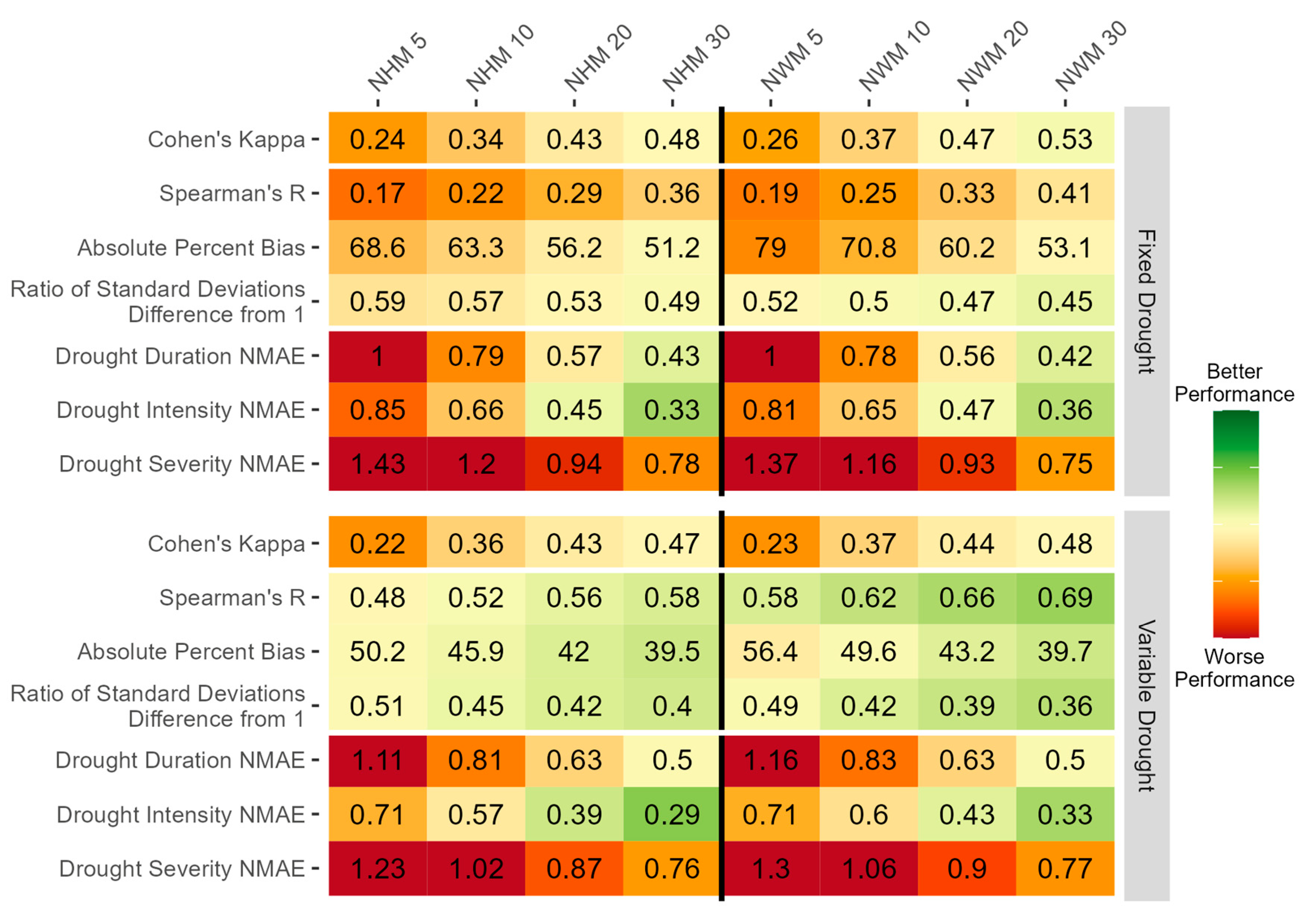
We present our systematic model evaluation results for each metric category in three sections: event classification (Section 3.1), error components (Section 3.2), and drought signatures (Section 3.3). Figure 2 presents a scorecard with an overview of the model performance across all metrics for each model, threshold, and drought characterization method, with more detailed results presented in the following sections. Detailed result data from this systematic evaluation are published for both the NWM [83] and the NHM [84], so that they may be used as benchmarks against which other hydrologic modeling applications can be compared.

3.1. Event Classification

The NWM and NHM simulated droughts had moderate agreement with the observed droughts (Cohen’s kappa 0.41–0.60) for the fixed and variable methods at the 20th and 30th thresholds, but had only fair agreement (0.21–0.40) when simulating more severe droughts (5th and 10th percentiles; Figure 2). This difference highlights that examining both the fixed and variable methods over a range of thresholds is necessary in relaying the range and patterns of performance. The NWM had slightly but consistently higher Cohen’s kappa values than the NHM across both methods (fixed and variable) and all thresholds of characterizing drought (Figure 2). Additionally, the difference in the Cohen’s kappa between thresholds (for both the fixed and variable methods) is substantially larger than the difference between the modeling applications, with the NWM only showing the slightly better detection of drought events than the NHM, but there is a two-fold increase in the median between the most extreme threshold (5th percentile) and most moderate threshold (30th percentile) for each model and each method. Both modeling applications classify drought events similarly for fixed and variable drought methods, although the models have slightly more agreement between stream gages for the fixed drought methods (Figure S2).
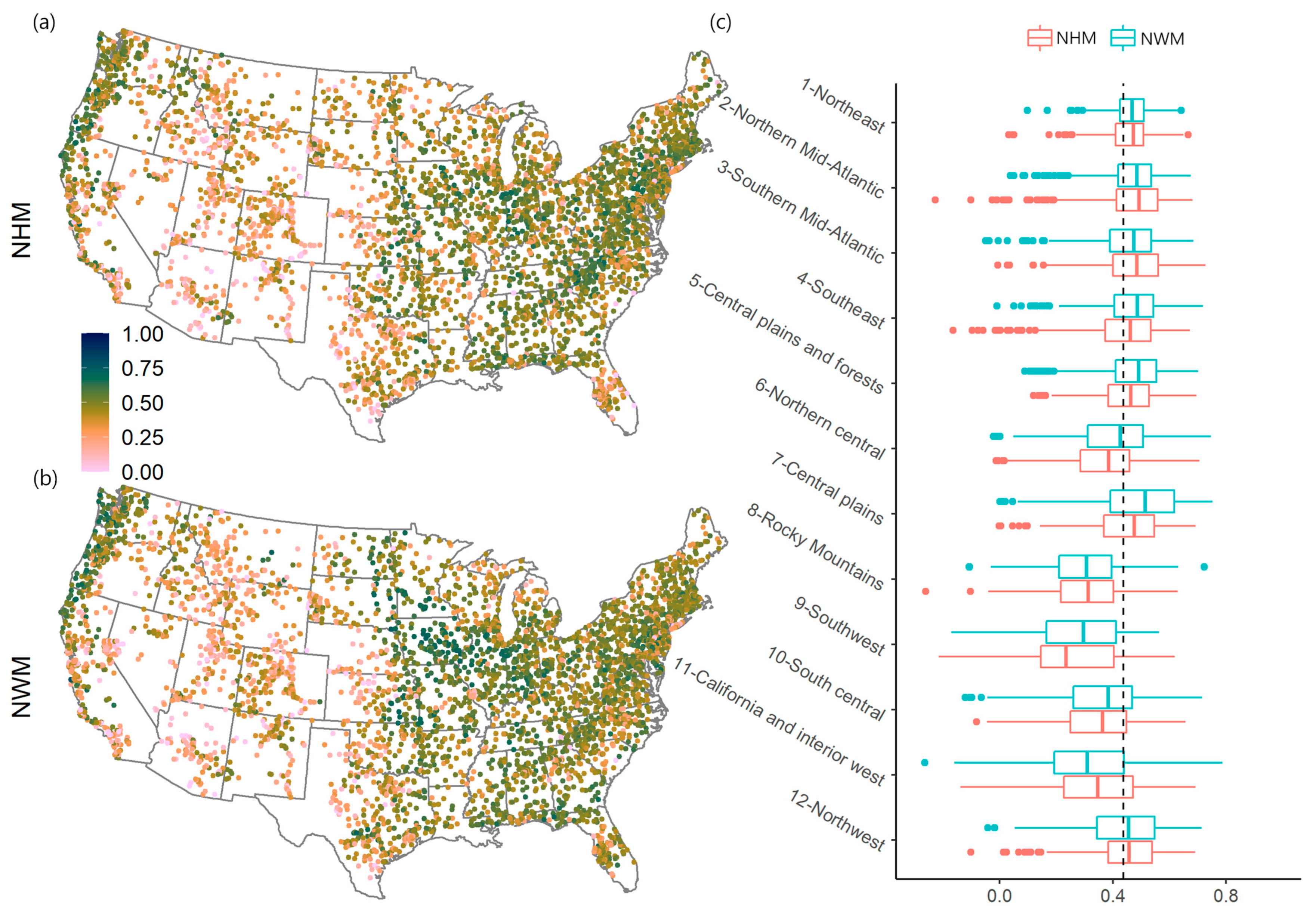
The examination of model performance over varying hydroclimatic regions is needed to understand if hydrologic models can generalize and classify streamflow drought well across large national scales. We found that the overall streamflow drought classification performance of the NHM and the NWM varies by region, with regions in the wetter, eastern CONUS typically showing the better classification of drought events than regions in the drier, western CONUS (Figure 3). This is consistent across percentile thresholds and drought classification methods. One exception to the generally poorer drought event classification in the west is the wetter, most northwestern region of CONUS (region 12). The northwest region has a Cohen’s kappa that is slightly higher than the national median for both the fixed and variable methods for the NHM and generally for the NWM, except for the 5th and 10th percentile fixed thresholds and the 30th percentile variable threshold.
There were some minor differences between the modeling applications in the west and east of CONUS, with the NHM classifying drought occurrence slightly more accurately than the NWM in the Northwest, California, and Interior West for all threshold types. The NWM classifies drought occurrence more accurately at the variable 20th percentile threshold than the NHM for much of central and eastern CONUS, but the NHM performs better in the Northwest and California and Interior West regions.
There was also more regional variability for the fixed threshold than the variable-threshold classification (Figure 3 and Figure S3). The NWM also outperforms the NHM in eastern regions by a wider margin for the fixed method. The median values for each approach were similar across all thresholds, with a Cohen’s kappa between 0.41 and 0.47 for the 20th percentile threshold.
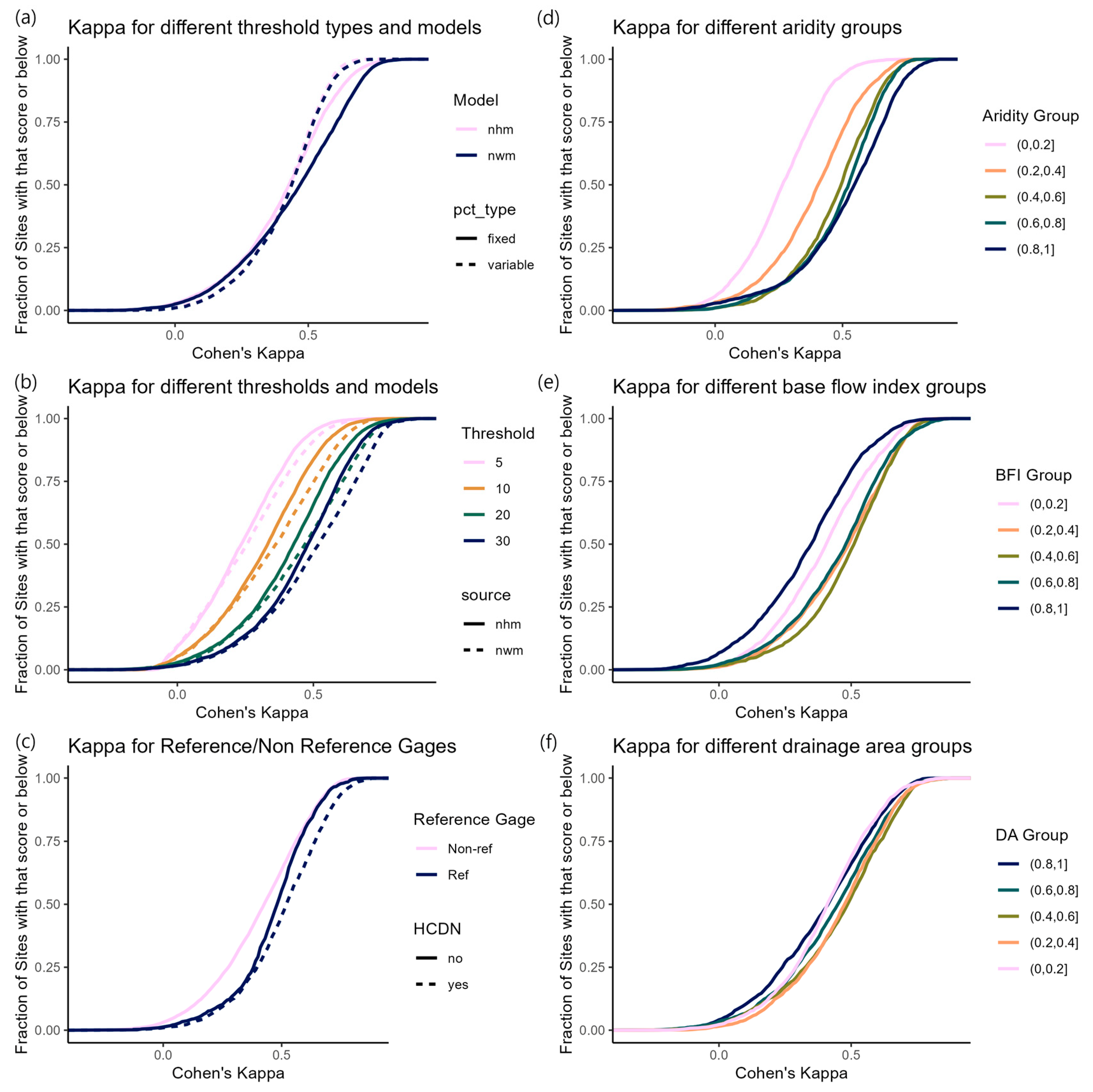
To further distinguish the model performance beyond regions, we examine the model performance across various basin characteristics like aridity, the drainage area, and the baseflow index (Figure 4; the baseflow index (BFI) is the long-term fractional contribution of subsurface flow to streamflow). Both modeling applications had a poorer performance with regards to classifying drought in more arid watersheds using the fixed and variable-threshold methods (Figure 4d and Figure S4). We found that both the NHM and NWM showed the worst simulations of drought occurrence for the 20% of stream gages with the highest BFI values (similar to [85,86]) and struggled for the 20% of stream gages with the lowest BFI (Figure 4e). The NHM and NWM also classified drought occurrence more accurately for moderate-sized basins (drainage area greater than 127.9 km2 and less than 3238 km2) than for the largest and smallest basins (Figure 4f).

3.2. Error Components

Across all thresholds, the Spearman’s r of the NWM was higher than that for the NHM, indicating that the NWM more accurately simulates the timing of streamflows during drought (Figure 2, Figures S5 and S6). Like drought classification, the differences in Spearman’s r between thresholds were larger than the differences between models for the fixed method (Figure 2). The timing of streamflows during drought was also more accurately simulated in wetter than dry regions. The NWM performs better in most regions, especially in the Northeast and Northern Mid-Atlantic regions, although the NHM does better in three out of the four westernmost regions (Northwest, Rocky Mountains, California and Interior West) for fixed-threshold drought (Figure S5). Both the NHM and NWM captured some of the timing of flows during the observed droughts, but not all, with overall moderate correlations for the variable threshold across percentile thresholds (NWM, 0.58–0.69; NHM 0.48–0.58; Figure 2; [87]). Performance for the fixed threshold was worse for both modeling applications, especially the more severe droughts (e.g., 5th percentile) where both models had relatively weak correlations with the observed flows during drought (NWM, 0.26; NHM 0.24).
Overall, the NWM had greater absolute bias than the NHM across all thresholds, indicating that the NHM more accurately simulates the streamflow volume during drought (Figure 2). Both modeling applications overestimate the streamflow during fixed drought (20th percentile threshold median percent bias across stream gages of 9.4% NHM, and 34% NWM), which is in line with previous studies indicating that models commonly overestimate low flows [88,89,90]. Both modeling applications have lower median percent biases for streamflow during variable drought, although this bias was much higher for the NWM (20th percentile threshold median percent bias of −3.3% NHM and 22% NWM; Equation (3)). Consistent with the lower median bias, the bias in the NHM was also more balanced across sites: many sites over or underestimate drought flows, whereas the NWM overestimates drought flows for most sites, particularly in the central CONUS (Figure 5). Between modeling applications, the differences in bias were larger for more extreme droughts (5th and 10th percentile thresholds) than for modest droughts (20th and 30th percentile thresholds) (Figure 2). Additionally, the biases for individual stream gages were not strongly correlated between modeling applications (correlation for fixed drought = 0.22, correlation for variable drought = 0.25). The percent bias varies substantially by region, with smaller absolute biases in the wetter Northeastern and Northwest regions, but larger positive biases for dry western regions (No. 6, 9, 10, and 11), especially for the NWM (Figure 5c and Figure S7c). While the median percent biases were well balanced across the CONUS for moderate droughts for the NHM and moderately overestimated flow for the NWM, it is important to note that the median absolute percent biases ranged from 39.5% for the 30th percentile NHM to 79% for the 5th percentile NWM (Figure 2) and that for certain stream gages, particularly in southwestern regions, the percent biases exceeded 400% (Figure 5).
Figure 4. Cumulative distributions of model performance at stream gages for Cohen’s kappa exploring model performance under a variety of different conditions and model groupings. Sub figures plot Cohen’s kappa comparing (a) the performance between the National Water Model (NWM) and the National Hydrologic Model (NHM) with fixed and variable methods, (b) the performance between the NWM and the NHM at 5th, 10th, 20th, and 30th percentile thresholds, (c) the performance at reference vs. non-reference [91] and Hydro-Climatic Data Network (HCDN) vs. non-HCDN gages, (d) the performance for various quantiles of aridity (Text S2), (e) the performance for various quantiles of the baseflow index (BFI; Text S2), and (f) the performance for various quantiles of drainage area (DA; Text S2). In cases where it is not explicit, the model performance is shown for the fixed method at the 20th percentile threshold combining both NWM and NHM evaluations.
Water 16 02996 g004
The difference in the ratio of standard deviations from its target value of 1 is higher for the NHM than for the NWM across all drought thresholds (Figure 2). There is relatively little agreement between each model’s ratio of standard deviations across stream g ages (fixed drought Spearman’s r = 0.27; variable drought Spearman’s r = 0.30). The spatial distributions of the ratio of standard deviations across the CONUS are variable (Figures S8 and S9). We generally see the lowest ratio of standard deviation differences between the modeling applications and the lowest variability among stream gages in the central eastern CONUS. The West, other than the Northwest, has high variability in the ratios of standard deviations across stream gages. The NWM tends to overestimate the variability of drought flows in these regions, while the NHM median ratio of standard deviations is close to 1. Both modeling applications tend to underestimate the variability in the Northeast.

3.3. Drought Signatures

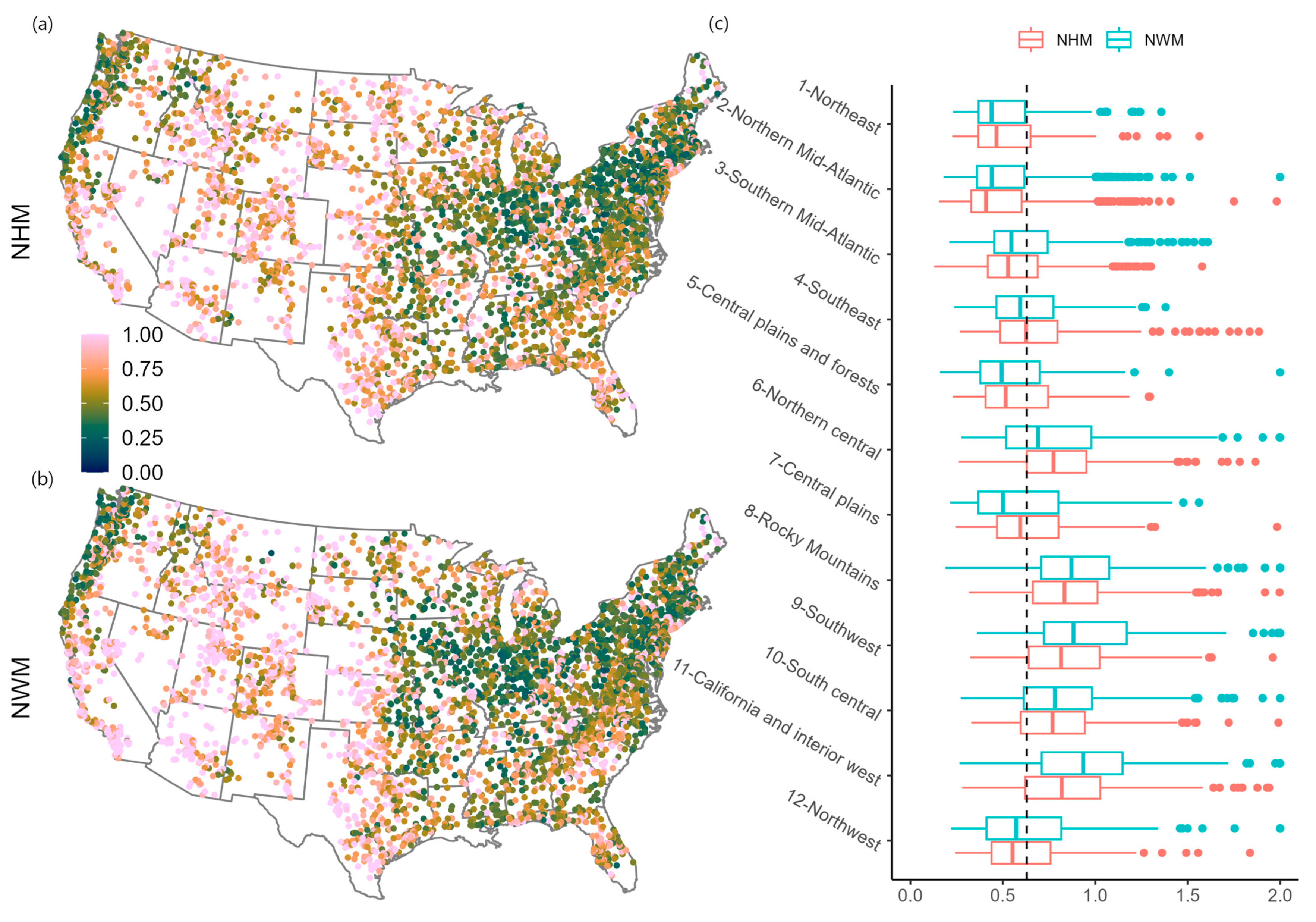
The NHM and the NWM perform similarly when simulating drought signatures, as measured by the NMAE values of the time sequence of the annual drought duration, intensity, and severity values, compared to the variability between different signature types and between different thresholds (Figure 2 and Figure 6). Generally, both modeling applications have lower errors for drought duration and intensity, and higher errors for drought severity (Figure 2).
Both the NHM and NWM simulate lower drought duration errors using fixed-threshold methods than variable-threshold methods (Figure 2). Despite an overall difference of less than 5% in the NMAE values for drought duration, the correlation between models at individual stream gages is only moderate (fixed drought correlation = 0.81; variable drought correlation = 0.76). Both modeling applications were better at simulating the drought duration in the eastern and northwestern CONUS than in other regions. The better model also varies from region to region. The NWM performs better than the NHM in the Central Plains, but worse in the Southwest and California and Interior West.
Across all percentile thresholds, both the NHM and NWM have higher errors for drought severity than for drought duration and drought intensity, especially in the California and Interior West, Rocky Mountains, and Northern central plains (Figures S10 and S11). The NWM better simulates drought severity using the fixed drought method, while the NHM better simulates drought severity using the variable drought method. Both the NHM and NWM perform better at the 20th percentile threshold than at lower thresholds. Agreement between the NWM and the NHM at individual stream gages is lower for severity than for other drought signatures (fixed drought correlation = 0.56; variable drought correlation = 0.64), likely because drought severity is a measure integrating drought duration and intensity and because our drought duration and intensity signatures are standardized (unitless), unlike our severity signature of flow volume, which is inherently correlated with basin size and flow. Model performance is better in the eastern CONUS than in the western CONUS, with many stream gages in the western CONUS having NMAEs much greater than 1 (Figure 6). When simulating drought severity, the NWM tends to outperform the NHM in wet regions (1, 2, 3, 4, and 12) while the NHM performs better in drier regions (5–11).
Simulations of drought intensity are generally better than those of drought duration. The NHM better simulates drought intensity for both the variable and the fixed 20th percentile thresholds. The NWM, however, better simulates the 5th and 10th percentile fixed-threshold drought intensity. The agreement between the NWM and NHM performance for individual stream gages is greater for variable drought intensity than it is for drought duration (fixed drought correlation = 0.80; variable drought correlation = 0.84). Similar patterns emerge with regard to regional model performance, with a better ability to simulate drought intensity in the Northeast and Northern Mid-Atlantic regions and a poor ability in the western CONUS, apart from the coastal Northwest. The variability in performance is much less for drought intensity than it is for drought severity. With the 20th percentile variable-threshold drought method, the NHM performs better or equal to the NWM in nearly all regions.
Overall, both modeling applications struggle to simulate drought signatures, with a NMAE greater than 50% for all signatures except drought duration at the 30th percentile threshold and drought intensity at the 30th and 20th percentile thresholds. Both modeling applications show high error when simulating drought severity, with NMAE values ranging from 0.76 for the NHM at the 30th percentile variable threshold to 1.43 at the NHM 5th percentile variable threshold.

4. Discussion

4.1. Tradeoffs in Specific Model Performance

Each model has distinct tradeoffs when it comes to simulating aspects of drought. The “better” model depends heavily on the defined drought threshold and the method for determining drought severity (fixed or variable). We generally found that the NWM better reproduces drought occurrence, as well as the timing and variability of flow during droughts (as measured by Cohen’s kappa, Spearman’s r, and the ratio of the standard deviations, respectively), whereas the NHM better reproduces drought intensity signatures (for moderate and variable drought). Though our findings are consistent with those of Towler et al. [24], the additional streamflow drought metrics used in this study are needed to provide deeper insight into the models’ performance during hydroclimatic drought that the low-flow percent bias metric in Yilmaz et al. [74] cannot provide alone.
Tradeoffs in performance for different streamflow error components like magnitude versus timing between hydrologic models are commonly identified in the literature, often with results similar to our findings. Gudmundsson et al. [92] similarly found distinct tradeoffs between models’ mean and correlation errors (like metrics of magnitude and timing we use) when simulating European annual runoff cycles. Similar types of tradeoffs extend to simulations of drought. Some of these differences may be due to different initial development priorities for each modeling application (see Towler et al. [24], for modeling application descriptions). For example, the development of the NWM has focused on flood prediction and operates at an hourly timestep [93,94,95]. This may be the reason why the NWM better simulates the timing of drought events than the NHM. Another consideration is that the NHM was designed for water availability assessments, with a focus on simulating water quantity or magnitude, and operates on a daily timestep [96]. The calibration of the NHM included a step for matching the water balance volumes within each modeling unit, another step with the identified headwater catchments being calibrated using several non-streamflow datasets and a statistically generated streamflow to target the timing of streamflow; finally, the observed streamflow is used within each headwater catchment as a final calibration step [43]. Spatial frameworks are often different between models, where the NWM runs on a 1 km grid, while the NHM is based on hydrologic response units. These differences may have impacts on model performance. The calibration focus on water balance may be the reason why the NHM is better able to simulate streamflow volumes during drought rather than the timing. In the broader perspective, it is important to recognize each model’s original purpose when interpreting the comparison results using these streamflow drought metrics, and generally any metrics used in benchmarking.

4.2. Model Performance Exhibits Regional Variation with Better Performance in Wetter Eastern Regions than in Drier Western Regions

The NWM and the NHM both simulate drought more poorly in drier western regions of the CONUS than in wetter eastern regions. Previous studies have also indicated poorer overall and drought-specific model simulations in the western CONUS [24,48,58]. Climate factors [92], including precipitation and aridity [58,97], have been widely found to influence model performance in different regions, so the poorer simulations of drought in drier regions are not surprising. These findings highlight an important area for model improvement since arid regions of the western CONUS are often the regions where drought is a major concern.
We also note that several important factors that influence the water cycle in western CONUS are not well captured by the hydrologic models used in this study. For example, human water use, diversions, and reservoir regulations, which are common throughout western watersheds [98], are not fully represented in either model. Additional processes that are not thoroughly represented, like lake and stream channel evaporation [99] or deep and complex groundwater systems [100], also may impact the model performance in the western CONUS. Other studies have shown that missing groundwater processes and not accounting for human modifications can result in poor model performance [73,101]. Benchmarking both models across our suite of metrics may help guide future development priorities in each model when looking to address issues such as the representation of human influences. If adding reservoir representation to the models, the NHM might benefit from more focus on the improved representation of the impacts of reservoirs on flow regime timing, as it had a poorer performance in simulating flow timing metrics (Spearman’s r) during drought relative to the NWM. The NWM, on the other hand, could potentially benefit from more focus on the improved representation of the flow magnitude impacts of reservoirs, as it had a poorer performance when simulating the flow magnitude (percent bias) during drought relative to the NHM.
The relative performance also varies spatially. For example, the NHM simulates drought occurrence (as measured by Cohen’s kappa) better in the western coastal regions (11 and 12) despite a worse national performance. In the southcentral CONUS, both modeling applications overestimate the magnitude and variability of drought flows by a large margin (like findings across all flows by Towler et al. [24]). Both modeling applications, especially the NWM, tend to better simulate the timing of flows during drought (Spearman’s r) in the southcentral CONUS, with values close to the national median. The Rocky Mountain region is the reverse: both modeling applications simulate the magnitude and variability of flows during drought similarly well to how they do in other regions, but Spearman’s r for both models is the lowest of all regions, which indicates difficulties simulating the timing of flows during drought in the Rocky Mountains. The regional differences in which the components of error each model perform well or poorly highlight some of the difficulties and potential tradeoffs between these models. Efforts focusing on improving the simulation of the magnitude of flows during drought may improve drought simulations for the southcentral CONUS, where the model has relatively high biases during periods of drought. In contrast, the Rocky Mountains, where the model simulations have a low Spearman’s r with observations, might benefit most from efforts focused on improving the simulations of flow timing during drought.
We see similar tradeoffs between metrics in regions where both modeling applications perform relatively better. The NWM and NHM simulate the timing, magnitude, and variability of flows during drought well in the northeastern CONUS with median statistical values that are either the highest or close to the highest compared to other regions. The NHM performs less well when simulating the occurrence of fixed-threshold drought in the northeast relative to some other regions like the Northern and Southern Mid-Atlantic (although Cohen’s kappa values are still at the national median). This indicates that the model’s simulations during periods of drought are good, but that the NHM may not always correctly indicate that there is a drought relative to the Mid-Atlantic regions, where the NHM better simulates drought occurrence.

4.3. Larger Differences in Performance Between Thresholds than Between Models Highlights the Importance of Using Consistent Benchmarking Methods

The differences in Cohen’s kappa, Spearman’s r, the drought duration, and drought severity was greater between thresholds than between modeling applications. Both the NHM and NWM performed worse for more extreme droughts. This may in part reflect similar deficiencies in the climate input data, the applicability of the model equations to arid regions, or the model parameterizations [24]. Once calibrated, models typically have less variance than the original observations, so they tend to overpredict low flows and underpredict high flows [102]. However, we did not see more modeled than observed variability within these drought periods, as measured by the ratio of standard deviations. Both modeling applications may be able to simulate the impact of flow generation processes on moderate drought flows (e.g., 20 and 30%) but have difficulties simulating the processes that drive extreme drought flows (e.g., 5 and 10%). Additionally, these severe flows are hard to calibrate as they occur infrequently.

4.4. Summary

The results show a varied performance between the modeling applications that differs based on the metric being evaluated, the method of identifying drought, and the region or stream gage of interest. These results suggest that these models can provide benefits and useful information in certain contexts and regions, particularly for more moderate droughts in high-performance regions like the eastern CONUS. Users of these modeling applications should exert caution because some evaluation metrics indicate potential issues. For example, some stream gages have percent biases over 400% during periods of drought and some have high NMAE values when simulating drought severity. These factors suggest that the model may be problematic for certain applications, particularly in capturing more severe droughts in certain regions of CONUS such as the drier western regions.
The systematic evaluation of these two modeling applications highlights differences in performance by metric and region. These differences, along with the larger differences between drought thresholds than between modeling applications for many performance statistics, show the importance of the systematic benchmarking of different models and the use of the same methods of drought identification when comparing models. It also shows the importance of evaluating a range of different thresholds, in a range of different regions, using various performance metrics.
The consistent finding that both modeling applications have difficulties in simulating more extreme drought and drought in more arid regions highlights the limitations of both models and suggests a need for continued modeling improvement, as also indicated by others [26,73]. The improved simulation of severe drought flows and drought in arid regions is critical as these flows have large social and ecological impacts. This need for improved simulation may become increasingly important as, in some of these arid regions, extreme drought flows may become more common with a changing climate [103]. It may be especially important for regions such as the Colorado River Basin that experience major droughts with substantial impacts across social and ecological systems in the region [104,105].

4.5. Limitations

This study helps improve the understanding of model performance in simulating drought events, but there are important limitations to note. Our assessment does not control for differences in the model calibration or forcing datasets, which influence the simulated results. For ideal comparisons of the underlying models, both modeling applications would use the same forcings and calibration techniques; however, this can be impracticable for large simulations as they are typically funded by different entities and created for somewhat different purposes. Similarly, the evaluation is performed on simulations at stream gages used for calibration and therefore does not assess out-sample errors, but it is likewise usually impractical in large-domain model implementations to perform the simulations needed to address this issue. Nevertheless, benchmarking the specific implementations of modeling applications or built-for-comparison modeling applications still gives insight into how each can be used for research and improvement. Our study assesses both fixed and variable methods of characterizing drought at four thresholds, but there are many other methods of characterizing streamflow drought that could yield different evaluation results. The autocorrelation of daily values is not considered in our study design, though this is critical to address if planning to perform statistical significance testing between modeling applications. Uncertainty in hydrologic simulations stems from several sources, including uncertainties in the input forcings, as well as from the hydrological model structure, process representation, absence of anthropogenic processes, and parameterization. Although we do not explicitly investigate model uncertainty nor their interactions here, we do note that we use two different hydrological models (NHM and NWM), which could be conducive to developing a multi-model ensemble; studies have shown that the ensemble mean can outperform individual models [106].

5. Conclusions

This study presents a comprehensive approach to evaluating simulations of streamflow drought and applies it to two conterminous U.S.-scale hydrologic modeling applications, the National Water Model (NWM) and the National Hydrologic Model (NHM). Our comparisons between the NWM and the NHM show varied results. The NWM tends to better simulate the timing of streamflow during drought events (measured by Spearman’s r) while the NHM tends to better simulate the magnitude of flow during drought events (measured by percent bias). There were also strong spatial trends in the drought simulation performance, with both the NHM and NWM performing better in wetter regions than drier ones, creating a stark east versus west divide in performance. Thus, both modeling applications perform worse in drought simulations for the regions that are most susceptible to drought. Finally, the differences in performance were typically greater between different drought thresholds than between either modeling application, with both the NHM and NWM exhibiting difficulties in simulating the most severe drought events.

Supplementary Materials

The following supporting information can be downloaded at: https://www.mdpi.com/article/10.3390/w16202996/s1, Text S1. Description of Metric Calculations. Text S2. Description of Aridity, Baseflow Index, Drainage Area, and HCDN and Reference Gage Calculations. Figure S1. Figure of our workflow of steps to characterize drought and evaluation model performance. Figure S2. Scatter plot figures comparing National Water Model (NWM) (x-axis) and National Hydrologic Model (NHM) (y-axis) performance for each metric at the 20th percentile threshold. Figure S3. Maps comparing drought event classification results using Cohen’s kappa. Figure S4. Cumulative distributions of model performance at stream gages for Cohen’s kappa exploring model performance for the National Hydrologic Model (NHM) and National Water Model (NWM) for fixed and variable drought methods, subset into groups based on the aridity quantiles. Figure S5. Maps comparing Spearman’s r of flows during drought. Figure S6. Maps comparing Spearman’s r of flows during drought. Figure S7. Maps comparing percent bias of flows during drought. Figure S8. Maps comparing the ratio of standard deviations of flows during drought. Figure S9. Maps comparing the ratio of standard deviations of flows during drought. Figure S10. Maps presenting the normalized mean absolute error. Figure S11. Maps presenting the normalized mean absolute error. Figure S12. Maps presenting the normalized mean absolute error. Figure S13. Maps presenting the normalized mean absolute error. Figure S14. Maps presenting the normalized mean absolute error.

Author Contributions

C.S.: Conceptualization, Data Curation, Formal Analysis, Methodology, Investigation, Writing—original draft, Writing—review and editing, Visualization, Project administration. S.F.: Conceptualization, Data Curation, Methodology, Investigation, Writing—original draft, Writing—review and editing, Project administration. E.T.: Conceptualization, Methodology, Writing—original draft, Writing—review and editing. T.H.: Conceptualization, Methodology, Writing—review and editing. T.O.: Conceptualization, Methodology, Writing—review and editing. All authors have read and agreed to the published version of the manuscript.

Funding

This research was supported by the U.S. Geological Survey Water Mission Area Hydro-terrestrial Earth System Testbed (HyTEST) project. Any use of trade, firm, or product names is for descriptive purposes only and does not imply endorsement by the U.S. Government.

Data Availability Statement

All data, software, and additional details of the methodology used in this study are publicly available from Simeone et al. [83,84] and Simeone and Foks [107].

Conflicts of Interest

The authors declare that they have no known competing financial interests or personal relationships that could have appeared to influence the work reported in this paper.

References

  1. Wlostowski, A.N.; Jennings, K.S.; Bash, R.E.; Burkhardt, J.; Wobus, C.W.; Aggett, G. Dry landscapes and parched economies: A review of how drought impacts nonagricultural socioeconomic sectors in the US Intermountain West. Wiley Interdiscip. Rev. Water 2022, 9, e1571. [Google Scholar] [CrossRef]
  2. Smith, A.B.; Matthews, J.L. Quantifying uncertainty and variable sensitivity within the US billion-dollar weather and climate disaster cost estimates. Nat. Hazards 2015, 77, 1829–1851. [Google Scholar] [CrossRef]
  3. NOAA. National Centers for Environmental Information (NCEI) U.S. Billion-Dollar Weather and Climate Disasters. Retrieved from Billion-Dollar Weather and Climate Disasters|National Centers for Environmental Information (NCEI); 2022. Available online: https://www.ncei.noaa.gov/access/billions/ (accessed on 1 October 2021).
  4. Hasan, H.H.; Razali, S.F.M.; Muhammad, N.S.; Ahmad, A. Research trends of hydrological drought: A systematic review. Water 2019, 11, 2252. [Google Scholar] [CrossRef]
  5. Van Huijgevoort, M.H.J.; Hazenberg, P.; Van Lanen, H.A.J.; Teuling, A.J.; Clark, D.B.; Folwell, S.; Gosling, S.N.; Hanasaki, N.; Heinke, J.; Koirala, S.; et al. Global multimodel analysis of drought in runoff for the second half of the twentieth century. J. Hydrometeorol. 2013, 14, 1535–1552. [Google Scholar] [CrossRef]
  6. Quintana-Seguí, P.; Barella-Ortiz, A.; Regueiro-Sanfiz, S.; Míguez-Macho, G. The Utility of Land-Surface Model Simulations to Provide Drought Information in a Water Management Context Using Global and Local Forcing Datasets. Water Resour. Manag. 2020, 34, 2135–2156. [Google Scholar] [CrossRef]
  7. Stahl, K.; Vidal, J.P.; Hannaford, J.; Tijdeman, E.; Laaha, G.; Gauster, T.; Tallaksen, L.M. The challenges of hydrological drought definition, quantification and communication: An interdisciplinary perspective. Proc. Int. Assoc. Hydrol. Sci. 2020, 383, 291–295. [Google Scholar] [CrossRef]
  8. Brunner, M.I.; Slater, L.; Tallaksen, L.M.; Clark, M. Challenges in modeling and predicting floods and droughts: A review. WIREs Water 2021, 8, e1520. [Google Scholar] [CrossRef]
  9. Rivera, J.A.; Infanti, J.M.; Kumar, R.; Mutemi, J.N. Challenges of Hydrological Drought Monitoring and Prediction. Front. Water 2021, 3, 750311. [Google Scholar] [CrossRef]
  10. Tallaksen, L.M.; Van Lanen, H.A. (Eds.) Hydrological Drought: Processes and Estimation Methods for Streamflow and Groundwater. 2004. Available online: https://hdl.handle.net/11311/1256137 (accessed on 1 October 2021).
  11. Van Loon, A.F. Hydrological drought explained. WIREs Water 2015, 2, 359–392. [Google Scholar] [CrossRef]
  12. Wilhite, D.A.; Glantz, M.H. Understanding the drought phenomenon: The role of definitions. Water Int. 1985, 10, 111–120. [Google Scholar] [CrossRef]
  13. Guo, Y.; Huang, S.; Huang, Q.; Wang, H.; Fang, W.; Yang, Y.; Wang, L. Assessing socioeconomic drought based on an improved multivariate standardized reliability and resilience index. J. Hydrol. 2019, 568, 904–918. [Google Scholar] [CrossRef]
  14. Mishra, A.K.; Singh, V.P. Drought modeling—A review. J. Hydrol. 2011, 403, 157–175. [Google Scholar] [CrossRef]
  15. Hao, Z.; Singh, V.P.; Xia, Y. Seasonal drought prediction: Advances, challenges, and future prospects. Rev. Geophys. 2018, 56, 108–141. [Google Scholar] [CrossRef]
  16. Smith, K.A.; Barker, L.J.; Tanguy, M.; Parry, S.; Harrigan, S.; Legg, T.P.; Prudhomme, C.; Hannaford, J. A multi-objective ensemble approach to hydrological modelling in the UK: An application to historic drought reconstruction. Hydrol. Earth Syst. Sci. 2019, 23, 3247–3268. [Google Scholar] [CrossRef]
  17. Fung, K.F.; Huang, Y.F.; Koo, C.H.; Soh, Y.W. Drought forecasting: A review of modelling approaches 2007–2017. J. Water Clim. Change 2020, 11, 771–799. [Google Scholar] [CrossRef]
  18. Sutanto, S.J.; Van Lanen, H.A. Streamflow drought: Implication of drought definitions and its application for drought forecasting. Hydrol. Earth Syst. Sci. 2021, 25, 3991–4023. [Google Scholar] [CrossRef]
  19. Dyer, J.; Mercer, A.; Raczyński, K. Identifying Spatial Patterns of Hydrologic Drought over the Southeast US Using Retrospective National Water Model Simulations. Water 2022, 14, 1525. [Google Scholar] [CrossRef]
  20. Yihdego, Y.; Vaheddoost, B.; Al-Weshah, R.A. Drought indices and indicators revisited. Arab. J. Geosci. 2019, 12, 69. [Google Scholar] [CrossRef]
  21. Faiz, M.A.; Zhang, Y.; Ma, N.; Baig, F.; Naz, F.; Niaz, Y. Drought indices: Aggregation is necessary or is it only the researcher’s choice? Water Supply 2021, 21, 3987–4002. [Google Scholar] [CrossRef]
  22. Alawsi, M.A.; Zubaidi, S.L.; Al-Bdairi, N.S.S.; Al-Ansari, N.; Hashim, K. Drought Forecasting: A Review and Assessment of the Hybrid Techniques and Data Pre-Processing. Hydrology 2022, 9, 115. [Google Scholar] [CrossRef]
  23. Archfield, S.A.; Clark, M.; Arheimer, B.; Hay, L.E.; McMillan, H.; Kiang, J.E.; Seibert, J.; Hakala, K.; Bock, A.; Wagener, T.; et al. Accelerating advances in continental domain hydrologic modeling. Water Resour. Res. 2015, 51, 10078–10091. [Google Scholar] [CrossRef]
  24. Towler, E.; Foks, S.S.; Dugger, A.L.; Dickinson, J.E.; Essaid, H.I.; Gochis, D.; Viger, R.J.; Zhang, Y. Benchmarking high-resolution hydrologic model performance of long-term retrospective streamflow simulations in the contiguous United States. Hydrol. Earth Syst. Sci. 2023, 27, 1809–1825. [Google Scholar] [CrossRef]
  25. Smakhtin, V.U. Low flow hydrology: A review. J. Hydrol. 2001, 240, 147–186. [Google Scholar] [CrossRef]
  26. Nicolle, P.; Pushpalatha, R.; Perrin, C.; François, D.; Thiéry, D.; Mathevet, T.; Le Lay, M.; Besson, F.; Soubeyroux, J.-M.; Viel, C.; et al. Benchmarking hydrological models for low-flow simulation and forecasting on French catchments. Hydrol. Earth Syst. Sci. 2014, 18, 2829–2857. [Google Scholar] [CrossRef]
  27. Hodgkins, G.A.; Dudley, R.W.; Russell, A.M.; LaFontaine, J.H. Comparing trends in modeled and observed streamflows at minimally altered basins in the United States. Water 2020, 12, 1728. [Google Scholar] [CrossRef]
  28. Mubialiwo, A.; Abebe, A.; Onyutha, C. Performance of rainfall–runoff models in reproducing hydrological extremes: A case of the River Malaba sub-catchment. SN Appl. Sci. 2021, 3, 515. [Google Scholar] [CrossRef]
  29. Worland, S.C.; Farmer, W.H.; Kiang, J.E. Improving predictions of hydrological low-flow indices in ungaged basins using machine learning. Environ. Model. Softw. 2018, 101, 169–182. [Google Scholar] [CrossRef]
  30. Pfannerstill, M.; Guse, B.; Fohrer, N. Smart low flow signature metrics for an improved overall performance evaluation of hydrological models. J. Hydrol. 2014, 510, 447–458. [Google Scholar] [CrossRef]
  31. Nash, J.E.; Sutcliffe, J.V. River flow forecasting through conceptual models part I—A discussion of principles. J. Hydrol. 1970, 10, 282–290. [Google Scholar] [CrossRef]
  32. Pushpalatha, R.; Perrin, C.; Le Moine, N.; Andreassian, V. A review of efficiency criteria suitable for evaluating low-flow simulations. J. Hydrol. 2012, 420, 171–182. [Google Scholar] [CrossRef]
  33. Dehghani, M.; Saghafian, B.; Rivaz, F.; Khodadadi, A. Evaluation of dynamic regression and artificial neural networks models for real-time hydrological drought forecasting. Arab. J. Geosci. 2017, 10, 266. [Google Scholar] [CrossRef]
  34. Barella-Ortiz, A.; Quintana-Seguí, P. Evaluation of drought representation and propagation in regional climate model simulations across Spain. Hydrol. Earth Syst. Sci. 2019, 23, 5111–5131. [Google Scholar] [CrossRef]
  35. Hammond, J.C.; Simeone, C.; Hecht, J.S.; Hodgkins, G.A.; Lombard, M.; McCabe, G.; Wolock, D.; Wieczorek, M.; Olson, C.; Caldwell, T.; et al. Going Beyond Low Flows: Streamflow Drought Deficit and Duration Illuminate Distinct Spatiotemporal Drought Patterns and Trends in the U.S. During the Last Century. Water Resour. Res. 2022, 58, e2022WR031930. [Google Scholar] [CrossRef]
  36. Heudorfer, B.; Stahl, K. Comparison of different threshold level methods for drought propagation analysis in Germany. Hydrol. Res. 2017, 48, 1311–1326. [Google Scholar] [CrossRef]
  37. Sarailidis, G.; Vasiliades, L.; Loukas, A. Analysis of streamflow droughts using fixed and variable thresholds. Hydrol. Process. 2019, 33, 414–431. [Google Scholar] [CrossRef]
  38. Jehanzaib, M.; Bilal Idrees, M.; Kim, D.; Kim, T.W. Comprehensive evaluation of machine learning techniques for hydrological drought forecasting. J. Irrig. Drain. Eng. 2021, 147, 04021022. [Google Scholar] [CrossRef]
  39. Collier, N.; Hoffman, F.M.; Lawrence, D.M.; Keppel-Aleks, G.; Koven, C.D.; Riley, W.J.; Mu, M.; Randerson, J.T. The International Land Model Benchmarking (ILAMB) System: Design, Theory, and Implementation. J. Adv. Model. Earth Syst. 2018, 10, 2731–2754. [Google Scholar] [CrossRef]
  40. Gochis, D.J.; Barlage, M.; Cabell, R.; Casali, M.; Dugger, A.; FitzGerald, K.; McAllister, M.; McCreight, J.; RafieeiNasab, A.; Read, L.; et al. The WRF-Hydro® Modeling System Technical Description, (Version 5.1.1). NCAR Technical Note. 2020. 107p. Available online: https://ral.ucar.edu/sites/default/files/public/projects/wrf-hydro/technical-description-user-guide/wrf-hydrov5.2technicaldescription.pdf (accessed on 1 October 2021).
  41. Regan, R.S.; Markstrom, S.L.; Hay, L.E.; Viger, R.J.; Norton, P.A.; Driscoll, J.M.; LaFontaine, J.H. Description of the national hydrologic model for use with the precipitation-runoff modeling system (prms) (No. 6-B9). In US Geological Survey Techniques and Methods; U.S. Geological Survey: Reston, VA, USA, 2018. [Google Scholar] [CrossRef]
  42. Hay, L.E.; LaFontaine, J.H. Application of the National Hydrologic Model Infrastructure with the Precipitation-Runoff Modeling System (NHM-PRMS), 1980–2016, Daymet Version 3 Calibration [Data Set]; U.S. Geological Survey: Reston, VA, USA, 2020. [CrossRef]
  43. Hay, L.E.; LaFontaine, J.H.; Van Beusekom, A.E.; Norton, P.A.; Farmer, W.H.; Regan, R.S.; Markstrom, S.L.; Dickinson, J.E. Parameter estimation at the conterminous United States scale and streamflow routing enhancements for the National Hydrologic Model infrastructure application of the Precipitation-Runoff Modeling System (NHM-PRMS). In U.S. Geological Survey Techniques and Methods; U.S. Geological Survey: Reston, VA, USA, 2023; Chapter B10; 50p. [Google Scholar] [CrossRef]
  44. Zhao, L. Event prediction in the big data era: A systematic survey. ACM Comput. Surv. (CSUR) 2021, 54, 1–37. [Google Scholar] [CrossRef]
  45. Cohen, J. A coefficient of agreement for nominal scales. Educ. Psychol. Meas. 1960, 20, 37–46. [Google Scholar] [CrossRef]
  46. Spearman, C. The Proof and Measurement of Association Between Two Things. In Studies in Individual Differences: The Search for Intelligence; Jenkins, J.J., Paterson, D.G., Eds.; Appleton-Century-Crofts: New York, NY, USA, 1961; pp. 45–58. [Google Scholar]
  47. Gupta, H.V.; Kling, H.; Yilmaz, K.K.; Martinez, G.F. Decomposition of the mean squared error and NSE performance criteria: Implications for improving hydrological modelling. J. Hydrol. 2009, 377, 80–91. [Google Scholar] [CrossRef]
  48. Hughes, M.; Jackson, D.L.; Unruh, D.; Wang, H.; Hobbins, M.; Ogden, F.L.; Cifelli, R.; Cosgrove, B.; DeWitt, D.; Dugger, A.; et al. Evaluation of retrospective National Water Model Soil moisture and streamflow for drought-monitoring applications. J. Geophys. Res. Atmos. 2024, 129, e2023JD038522. [Google Scholar] [CrossRef]
  49. Addor, N.; Do, H.X.; Alvarez-Garreton, C.; Coxon, G.; Fowler, K.; Mendoza, P.A. Large-sample hydrology: Recent progress, guidelines for new datasets and grand challenges. Hydrol. Sci. J. 2020, 65, 712–725. [Google Scholar] [CrossRef]
  50. Bales, R.C.; Goulden, M.L.; Hunsaker, C.T.; Conklin, M.H.; Hartsough, P.C.; O’Geen, A.T.; Hopmans, J.W.; Safeeq, M. Mechanisms controlling the impact of multi-year drought on mountain hydrology. Sci. Rep. 2018, 8, 690. [Google Scholar] [CrossRef] [PubMed]
  51. Gupta, H.V.; Perrin, C.; Blöschl, G.; Montanari, A.; Kumar, R.; Clark, M.; Andréassian, V. Large-sample hydrology: A need to balance depth with breadth. Hydrol. Earth Syst. Sci. 2014, 18, 463–477. [Google Scholar] [CrossRef]
  52. Thornton, P.E.; Thornton, M.M.; Mayer, B.W.; Wei, Y.; Devarakonda, R.; Vose, R.S.; Cook, R.B. Daymet: Daily Surface Weather Data on a 1-km Grid for North America, Version 3; ORNL DAAC: Oak Ridge, TN, USA, 2017. [Google Scholar] [CrossRef]
  53. Fall, G.; Kitzmiller, D.; Pavlovic, S.; Zhang, Z.; Patrick, N.; St. Laurent, M.; Trypaluk, C.; Wu, W.; Miller, D. The Office of Water Prediction’s Analysis of Record for Calibration, version 1.1: Dataset description and precipitation evaluation. JAWRA J. Am. Water Resour. Assoc. 2023, 59, 1246–1272. [Google Scholar] [CrossRef]
  54. Krause, P.; Boyle, D.P.; Base, F. Comparison of different efficiency criteria for hydrological model assessment. Adv. Geosci. 2005, 5, 89–97. [Google Scholar] [CrossRef]
  55. Gochis, D.J.; Cosgrove, B.; Dugger, A.L.; Karsten, L.; Sampson, K.M.; McCreight, J.L.; Flowers, T.; Clark, E.P.; Vukicevic, T.; Salas, F.R.; et al. Multi-variate evaluation of the NOAA National Water Model. In AGU Fall Meeting; NSF National Center for Atmospheric Research: Boulder, CO, USA, 2018. [Google Scholar]
  56. Lahmers, T.M.; Hazenberg, P.; Gupta, H.; Castro, C.; Gochis, D.; Dugger, A.; Yates, D.; Read, L.; Karsten, L.; Wang, Y.-H. Evaluation of NOAA National Water Model Parameter Calibration in Semiarid Environments Prone to Channel Infiltration. J. Hydrometeorol. 2021, 22, 2939–2969. [Google Scholar]
  57. Hodgkins, G.A.; Over, T.M.; Dudley, R.W.; Russell, A.M.; LaFontaine, J.H. The consequences of neglecting reservoir storage in national-scale hydrologic models: An appraisal of key streamflow statistics. J. Am. Water Resour. Assoc. 2023, 60, 110–131. [Google Scholar] [CrossRef]
  58. Johnson, J.M.; Fang, S.; Sankarasubramanian, A.; Rad, A.M.; da Cunha, L.K.; Jennings, K.S.; Clarke, K.C.; Mazrooei, A.; Yeghiazarian, L. Comprehensive analysis of the NOAA National Water Model: A call for heterogeneous formulations and diagnostic model selection. J. Geophys. Res. Atmos. 2023, 128, e2023JD038534. [Google Scholar] [CrossRef]
  59. Foks, S.S.; Towler, E.; Hodson, T.O.; Bock, A.R.; Dickinson, J.E.; Dugger, A.L.; Dunne, K.A.; Essaid, H.I.; Miles, K.A.; Over, T.M.; et al. Streamflow benchmark locations for conterminous United States (cobalt gages). In U.S. Geological Survey Data Release; U.S. Geological Survey: Reston, VA, USA, 2022. [Google Scholar] [CrossRef]
  60. Carpenter, D.H.; Hayes, D.C. Low-flow characteristics of streams in Maryland and Delaware. Water-Resour. Investig. Rep. 1996, 94, 4020. [Google Scholar]
  61. Feaster, T.D.; Lee, K.G. Low-flow frequency and flow-duration characteristics of selected streams in Alabama through March 2014. In U.S. Geological Survey Scientific Investigations Report 2017–5083; U.S. Geological Survey: Reston, VA, USA, 2017; 371p. [Google Scholar] [CrossRef]
  62. Lins, H.F. USGS hydro-climatic data network 2009 (HCDN-2009). In US Geological Survey Fact; U.S. Geological Survey: Reston, VA, USA, 2012; Sheet 2012-3047. [Google Scholar]
  63. McCabe, G.J.; Wolock, D.M. Clusters of monthly streamflow values with similar temporal patterns at 555 HCDN (Hydro-Climatic Data Network) sites for the period 1981 to 2019. In U.S. Geological Survey Data Release; U.S. Geological Survey: Reston, VA, USA, 2022. [Google Scholar] [CrossRef]
  64. Laaha, G.; Gauster, T.; Tallaksen, L.M.; Vidal, J.P.; Stahl, K.; Prudhomme, C.; Heudorfer, B.; Vlnas, R.; Ionita, M.; Van Lanen, H.A.J.; et al. The European 2015 drought from a hydrological perspective. Hydrol. Earth Syst. Sci. 2017, 21, 3001–3024. [Google Scholar] [CrossRef]
  65. Simeone, C.E. Streamflow Drought Metrics for select GAGES-II streamgages for three different time periods from 1921–2020. In U.S. Geological Survey Data Release; U.S. Geological Survey: Reston, VA, USA, 2022. [Google Scholar] [CrossRef]
  66. Van Huijgevoort, M.H.J.; Hazenberg, P.; Van Lanen, H.A.J.; Uijlenhoet, R. A generic method for hydrological drought identification across different climate regions. Hydrol. Earth Syst. Sci. 2012, 16, 2437–2451. [Google Scholar] [CrossRef]
  67. Landis, J.R.; Koch, G.G. The measurement of observer agreement for categorical data. Biometrics 1977, 33, 159–174. [Google Scholar] [CrossRef] [PubMed]
  68. Clark, M.P.; Vogel, R.M.; Lamontagne, J.R.; Mizukami, N.; Knoben, W.J.; Tang, G.; Gharari, S.; Freer, J.E.; Whitfield, P.H.; Shook, K.R.; et al. The abuse of popular performance metrics in hydrologic modeling. Water Resour. Res. 2021, 57, e2020WR029001. [Google Scholar] [CrossRef]
  69. Hodson, T.O.; Over, T.M.; Foks, S.S. Mean squared error, deconstructed. J. Adv. Model. Earth Syst. 2021, 13, e2021MS002681. [Google Scholar] [CrossRef]
  70. Helsel, D.R.; Hirsch, R.M.; Ryberg, K.R.; Archfield, S.A.; Gilroy, E.J. Statistical methods in water resources. In U.S. Geological Survey Techniques and Methods; [Supersedes USGS Techniques of Water-Resources Investigations, Book 4, Chapter A3, version 1.1.]; U.S. Geological Survey: Reston, VA, USA, 2020; Book 4, Chapter A3; 458p. [Google Scholar] [CrossRef]
  71. Yue, S.; Pilon, P.; Cavadias, G. Power of the Mann-Kendall and Spearman’s rho tests for detecting monotonic trends in hydrological series. J. Hydrol. 2002, 259, 254–271. [Google Scholar] [CrossRef]
  72. Barber, C.; Lamontagne, J.R.; Vogel, R.M. Improved estimators of correlation and R2 for skewed hydrologic data. Hydrol. Sci. J. 2020, 65, 87–101. [Google Scholar] [CrossRef]
  73. Tijerina-Kreuzer, D.; Condon, L.; FitzGerald, K.; Dugger, A.; O’neill, M.M.; Sampson, K.; Gochis, D.; Maxwell, R. Continental hydrologic intercomparison project, phase 1: A large-scale hydrologic model comparison over the continental United States. Water Resour. Res. 2021, 57, e2020WR028931. [Google Scholar] [CrossRef]
  74. Yilmaz, K.K.; Gupta, H.V.; Wagener, T. A process-based diagnostic approach to model evaluation: Application to the NWS distributed hydrologic model. Water Resour. Res. 2008, 44. [Google Scholar] [CrossRef]
  75. Newman, A.J.; Mizukami, N.; Clark, M.P.; Wood, A.W.; Nijssen, B. Benchmarking of a physically based hydrologic model. J. Hydrometeorol. 2017, 18, 2215–2225. [Google Scholar] [CrossRef]
  76. Yevjevich, V.M. An Objective Approach to Definitions and Investigations of Continental Hydrologic Droughts; Colorado State University: Fort Collins, CO, USA, 1967; Volume 23, p. 25. [Google Scholar]
  77. Dracup, J.A.; Lee, K.S.; Paulson, E.G., Jr. On the statistical characteristics of drought events. Water Resour. Res. 1980, 16, 289–296. [Google Scholar] [CrossRef]
  78. Mishra, A.K.; Singh, V.P. A review of drought concepts. J. Hydrol. 2010, 391, 202–216. [Google Scholar] [CrossRef]
  79. Noel, M.; Bathke, D.; Fuchs, B.; Gutzmer, D.; Haigh, T.; Hayes, M.; Poděbradská, M.; Shield, C.; Smith, K.; Svoboda, M. Linking drought impacts to drought severity at the state level. Bull. Am. Meteorol. Soc. 2020, 101, E1312–E1321. [Google Scholar] [CrossRef]
  80. Addor, N.; Nearing, G.; Prieto, C.; Newman, A.J.; Le Vine, N.; Clark, M.P. A ranking of hydrological signatures based on their predictability in space. Water Resour. Res. 2018, 54, 8792–8812. [Google Scholar] [CrossRef]
  81. McMillan, H.K. A review of hydrologic signatures and their applications. WIREs Water 2021, 8, e1499. [Google Scholar] [CrossRef]
  82. Pournasiri Poshtiri, M.; Towler, E.; Pal, I. Characterizing and understanding the variability of streamflow drought indicators within the USA. Hydrol. Sci. J. 2018, 63, 1791–1803. [Google Scholar] [CrossRef]
  83. Simeone, C.; Leah, S.; Katharine, K. Results of benchmarking National Water Model v2.1 simulations of streamflow drought duration, severity, deficit, and occurrence in the conterminous United States. In U.S. Geological Survey Data Release; U.S. Geological Survey: Reston, VA, USA, 2024. [Google Scholar]
  84. Simeone, C.; Leah, S.; Katharine, K. Results of benchmarking National Hydrologic Model application of the Precipitation-Runoff Modeling System (v1.0 byObsMuskingum) simulations of streamflow drought duration, severity, deficit, and occurrence in the conterminous United States. In U.S. Geological Survey Data Release; U.S. Geological Survey: Reston, VA, USA, 2024; Chapter B10; 50p. [Google Scholar]
  85. Rudd, A.C.; Bell, V.A.; Kay, A.L. National-scale analysis of simulated hydrological droughts (1891–2015). J. Hydrol. 2017, 550, 368–385. [Google Scholar] [CrossRef]
  86. Massmann, C. Identification of factors influencing hydrologic model performance using a top-down approach in a large number of US catchments. Hydrol. Process. 2020, 34, 4–20. [Google Scholar] [CrossRef]
  87. Overholser, B.R.; Sowinski, K.M. Biostatistics primer: Part 2. Nutr. Clin. Pract. 2008, 23, 76–84. [Google Scholar] [CrossRef]
  88. Farmer, W.H.; Vogel, R.M. On the deterministic and stochastic use of hydrologic models. Water Resour. Res. 2016, 52, 5619–5633. [Google Scholar] [CrossRef]
  89. Moges, E.; Ruddell, B.L.; Zhang, L.; Driscoll, J.M.; Norton, P.; Perez, F.; Larsen, L.G. HydroBench: Jupyter supported reproducible hydrological model benchmarking and diagnostic tool. Front. Earth Sci. 2022, 10, 884766. [Google Scholar] [CrossRef]
  90. Wan, T.; Covert, B.H.; Kroll, C.N.; Ferguson, C.R. An Assessment of the National Water Model’s Ability to Reproduce Drought Series in the Northeastern United States. J. Hydrometeorol. 2022, 23, 1929–1943. [Google Scholar] [CrossRef]
  91. Falcone, J.A. GAGES-II: Geospatial Attributes of Gages for Evaluating Streamflow; U.S. Geological Survey: Reston, VA, USA, 2011. [CrossRef]
  92. Gudmundsson, L.; Wagener, T.; Tallaksen, L.M.; Engeland, K. Evaluation of nine large-scale hydrological models with respect to the seasonal runoff climatology in Europe: Land Surface Models Evaluation. Water Resour. Res. 2012, 48. [Google Scholar] [CrossRef]
  93. Maidment, D.R. Conceptual Framework for the National Flood Interoperability Experiment. J. Am. Water Resour. Assoc. 2016, 53, 245–257. [Google Scholar] [CrossRef]
  94. NOAA. National Water Model CONUS Retrospective Dataset. Available online: https://registry.opendata.aws/nwm-archive (accessed on 1 October 2021).
  95. UCAR. Supporting the NOAA National Water Model. 2019. Available online: https://ral.ucar.edu/projects/supporting-the-noaa-national-water-model (accessed on 1 October 2021).
  96. Regan, R.S.; Juracek, K.E.; Hay, L.E.; Markstrom, S.L.; Viger, R.J.; Driscoll, J.M.; LaFontaine, J.H.; Norton, P.A. The US Geological Survey National Hydrologic Model infrastructure: Rationale, description, and application of a watershed-scale model for the conterminous United States. Environ. Model. Softw. 2019, 111, 192–203. [Google Scholar] [CrossRef]
  97. Hansen, C.; Shiva, J.S.; McDonald, S.; Nabors, A. Assessing retrospective National Water Model streamflow with respect to droughts and low flows in the Colorado River basin. JAWRA J. Am. Water Resour. Assoc. 2019, 55, 964–975. [Google Scholar] [CrossRef]
  98. Carlisle, D.; Wolock, D.M.; Konrad, C.P.; McCabe, G.J.; Eng, K.; Grantham, T.E.; Mahler, B. Flow Modification in the Nation’s Streams and Rivers; US Department of the Interior, US Geological Survey: Reston, VA, USA, 2019.
  99. Friedrich, K.; Grossman, R.L.; Huntington, J.; Blanken, P.D.; Lenters, J.; Holman, K.D.; Gochis, D.; Livneh, B.; Prairie, J.; Skeie, E.; et al. Reservoir evaporation in the Western United States: Current science, challenges, and future needs. Bull. Am. Meteorol. Soc. 2018, 99, 167–187. [Google Scholar] [CrossRef]
  100. Hare, D.K.; Helton, A.M.; Johnson, Z.C.; Lane, J.W.; Briggs, M.A. Continental-scale analysis of shallow and deep groundwater contributions to streams. Nat. Commun. 2021, 12, 1450. [Google Scholar] [CrossRef]
  101. Lane, R.A.; Coxon, G.; Freer, J.E.; Wagener, T.; Johnes, P.J.; Bloomfield, J.P.; Greene, S.; Macleod, C.J.A.; Reaney, S.M. Benchmarking the predictive capability of hydrological models for river flow and flood peak predictions across over 1000 catchments in Great Britain. Hydrol. Earth Syst. Sci. 2019, 23, 4011–4032. [Google Scholar] [CrossRef]
  102. Vogel, R.M. Editorial: Stochastic and deterministic world views. J. Water Resour. Plan. Manag. 1999, 125, 311–313. [Google Scholar] [CrossRef]
  103. Ahmadalipour, A.; Moradkhani, H.; Svoboda, M. Centennial drought outlook over the CONUS using NASA-NEX downscaled climate ensemble. Int. J. Climatol. 2017, 37, 2477–2491. [Google Scholar] [CrossRef]
  104. Salehabadi, H.; Tarboton, D.G.; Udall, B.; Wheeler, K.G.; Schmidt, J.C. An Assessment of Potential Severe Droughts in the Colorado River Basin. J. Am. Water Resour. Assoc. 2022, 58, 1053–1075. [Google Scholar] [CrossRef]
  105. Williams, A.P.; Cook, B.I.; Smerdon, J.E. Rapid intensification of the emerging southwestern North American megadrought in 2020–2021. Nat. Clim. Chang. 2022, 12, 232–234. [Google Scholar] [CrossRef]
  106. Xia, Y.; Mitchell, K.; Ek, M.; Cosgrove, B.; Sheffield, J.; Luo, L.; Alonge, C.; Wei, H.; Meng, J.; Livneh, B.; et al. Continental-scale water and energy flux analysis and validation for North American Land Data Assimilation System project phase 2 (NLDAS-2): 2. Validation of model-simulated streamflow. J. Geophys. Res. Atmos. 2012, 117, D03110. [Google Scholar] [CrossRef]
  107. Simeone, C.E.; Foks, S.S. HyMED—Hydrologic Model Evaluation for Drought: R package version 1.0.0. In U.S. Geological Survey Software Release; U.S. Geological Survey: Reston, VA, USA, 2024. [Google Scholar]
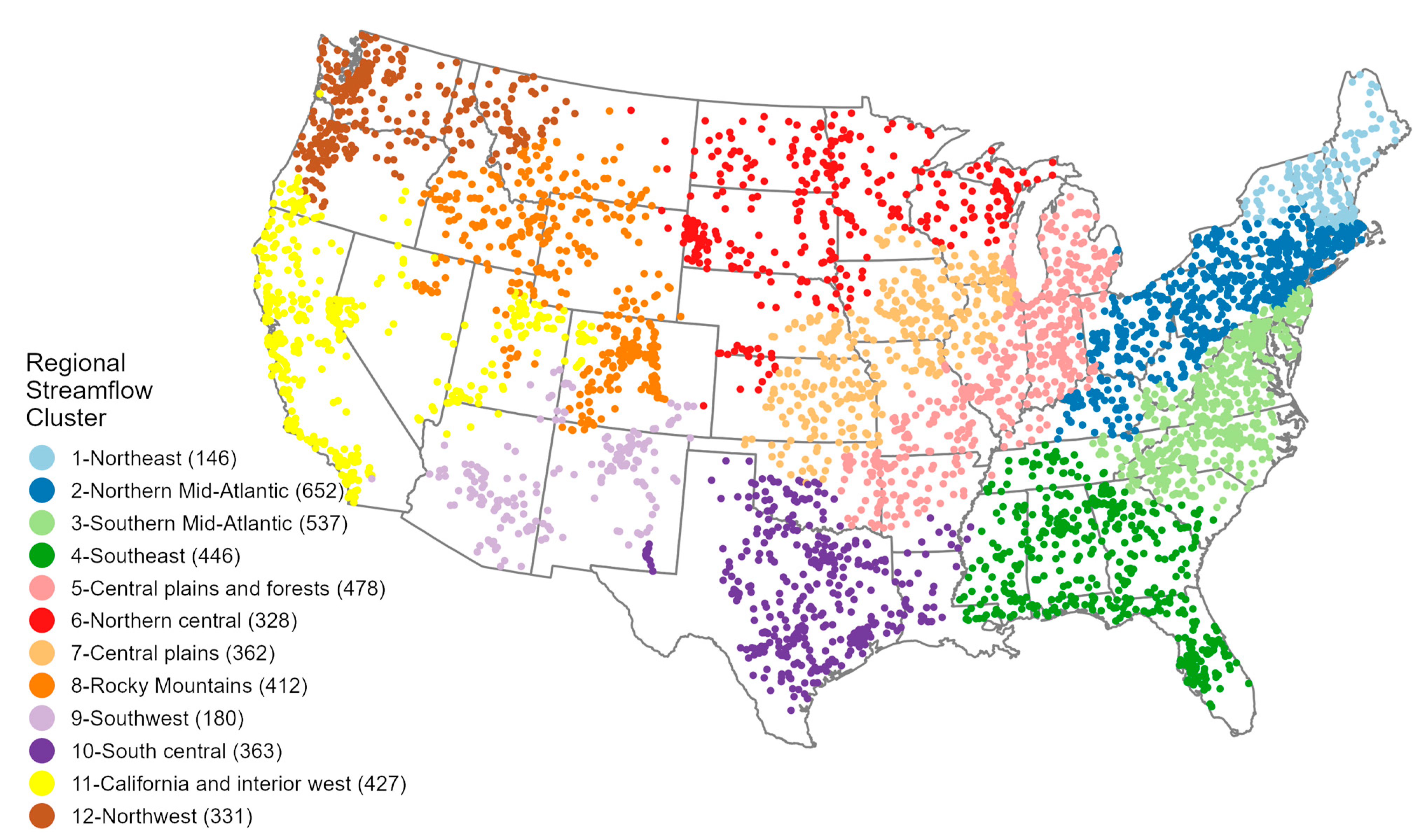
Figure 1. Streamflow gages (n = 4662) colored by regional streamflow cluster. The number of stream gages in each region is in parentheses.
Water 16 02996 g001
Figure 2. Scorecard comparing median model evaluation results for the National Water Model (NWM) and the National Hydrologic Model (NHM). The scorecard columns are the models at each of the 5th, 10th, 20th, or 30th streamflow percentile thresholds. The rows are the metric categories of drought, namely event classification, error components, and drought signatures (Table 1), for fixed (top) and variable (bottom) drought methods. The metric values are in the corresponding box. Greener box colors indicate better performance, whereas redder box colors indicate poorer performance. Percent bias is the absolute value of percent bias. The ratio of standard deviations is the absolute difference in the ratio of standard deviations from 1. Drought signatures are the normalized mean absolute error (NMAE) of drought duration, intensity, and severity.
Water 16 02996 g002
Figure 3. Maps comparing drought event classification results using Cohen’s kappa for (a) the National Hydrologic Model (NHM) and (b) the National Water Model (NWM) for the variable drought method at the 20th percentile threshold. Darker colors indicate more agreement. The (c) box plot shows the results by region. The y-axes represent the 12 regions described in Figure 1. The x-axes represent the respective Cohen’s kappa values. The NWM is in blue. The NHM is in red. The vertical black line is the median statistic value across all stream gages for both models. The event classification results using the fixed drought method are presented in the Supplementary Materials.
Water 16 02996 g003
Figure 5. Maps comparing the percent bias of flows during drought for (a) the National Hydrologic Model (NHM) and (b) the National Water Model (NWM) for the variable drought method at the 20th percentile threshold. Lighter points indicate better results, while blue represents overestimates and red represents underestimates of flow. The (c) box plot shows results by region. The y-axis represents the 12 regions described in Figure 1. The x-axis represents the respective percent bias values. The NWM is in blue. The NHM is in red. The vertical black line is the median statistic value across all stream gages. Note that boxplot values can be above or below the target for the statistic. Additional error component results are shown in the Supplemental Information for Spearman’s r using fixed (Figure S5) and variable methods (Figure S6), the percent bias using a fixed method (Figure S7), and the ratio of standard deviations using fixed (Figure S8) and variable methods (Figure S9).
Water 16 02996 g005
Figure 6. Maps presenting the normalized mean absolute error for (a) the National Hydrologic Model (NHM) and (b) the National Water Model (NWM) annual drought duration signature calculated with the variable drought method at the 20th percentile threshold. Darker colors represent lower errors between simulated and observed data. The (c) box plot shows the results by region. The y-axes represent the 12 regions described in Figure 1. The x-axes represent the normalized mean absolute error values. The NWM is in blue. The NHM is in red. The vertical black line is the median statistical value across all stream gages. Additional drought signature results are shown in the Supplemental Information for drought severity using fixed (Figure S10) and variable methods (Figure S11), drought intensity using fixed (Figure S12) and variable methods (Figure S13), and drought duration using a fixed method (Figure S14).
Water 16 02996 g006
Table 1. Streamflow drought statistical metrics for daily streamflow drought evaluation for different metric categories. Additional calculation details can be found in Text S1.
CategoryStatisticDescriptionRange (Perfect)Comments
Event
Classification
Cohen’s kappaCohen’s kappa statistic for inter-rater reliability [45]−1 to 1 (1)A measure of agreement relative to the probability of achieving results by chance.
Error
Components
Spearman’s rSpearman’s rank correlation coefficient−1 to 1 (1)A nonparametric estimator of correlation for flow timing.
Ratio of standard deviationsRatio of simulated to observed standard deviations (for the scorecard this is presented as the absolute deviation from the target of 1)0 to Inf (1)Indicates if the flow variability is being over or underestimated.
Percent biasPercent bias (simulated minus observed) (for the scorecard this is presented as the absolute percent bias)−100 to Inf (0)Indicates if total streamflow volume is being over or underestimated.
Drought
Signatures
Drought
Duration
Normalized mean absolute error (NMAE) in the annual time series of drought duration, i.e., the sum of days of drought each year for a given threshold.0 to Inf (0)Indicates how well the model simulates annual drought durations.
Drought
Intensity
NMAE in the annual time series of the distance the minimum percentile is below the drought threshold, i.e., the overall maximum distance below the threshold for any drought during the year.0 to Inf (0)Indicates how well the model simulates annual minimum flow.
Drought Severity (Flow Deficit Volume)NMAE in the annual time series of drought deficit volume in cubic meters per second-days (cms-days), i.e., the sum of drought deficits for all droughts during the year.0 to Inf (0)Indicates how well the model simulates annual flow deficit. This is a measure of drought severity.
Disclaimer/Publisher’s Note: The statements, opinions and data contained in all publications are solely those of the individual author(s) and contributor(s) and not of MDPI and/or the editor(s). MDPI and/or the editor(s) disclaim responsibility for any injury to people or property resulting from any ideas, methods, instructions or products referred to in the content.