Article

Sensitivity and Uncertainty Analysis of the GeeSEBAL Model Using High-Resolution Remote-Sensing Data and Global Flux Site Data

1
State Key Laboratory of Desert and Oasis Ecology, Xinjiang Institute of Ecology and Geography, Chinese Academy of Sciences, Urumqi 830000, China
2
National Field Scientific Observation and Research Station of Akesu Oasis Farmland Ecosystem, Aksu 843000, China
3
School of Resources and Environment, University of Chinese Academy of Sciences, Beijing 100001, China
*
Author to whom correspondence should be addressed.
Water 2024, 16(20), 2978; https://doi.org/10.3390/w16202978
Submission received: 20 June 2024 / Revised: 12 October 2024 / Accepted: 14 October 2024 / Published: 18 October 2024
(This article belongs to the Special Issue Agricultural Water-Land-Plant System Engineering)

Abstract

:
Actual evapotranspiration (ETa) is an important component of the surface water cycle. The geeSEBAL model is increasingly being used to estimate ETa using high-resolution remote-sensing data (Landsat 4/5/7/8). However, due to surface heterogeneity, there is significant uncertainty. By optimizing the quantile values of the reverse-modelling automatic calibration algorithm (CIMEC) endpoint-component selection algorithm under extreme conditions through 212 global flux sites, we obtained the optimized quantile values of 11 vegetation types of cold- and hot-pixel endpoint components (Ts and NDVI). Based on the observation data of the global FLUXNET tower, the sensitivity of 20 parameters in the improved geeSEBAL model was determined through Sobol’s sensitivity analysis. Among them, the parameters dT and SAVI,hot were confirmed as the most sensitive parameters of the algorithm. Subsequently, we used the differential evolution Markov chain (DE-MC) method to analyse the uncertainty of the parameters in the geeSEBAL model used the posterior distribution of the parameters to modify the sensitive parameter values or ranges in the improved geeSEBAL model and to simulate the daily ETa. The results indicate that by analysing the end element components of the geeSEBAL model (Ts and NDVI), quantile numerical optimization and parameter optimization can be performed. Compared with the original algorithm, the improved geeSEBAL model has significantly improved simulation performance, as shown by higher R2 values, higher NSE values, smaller bias values, and lower RMSE values. The most suitable values of the predefined parameter Zoh were determined, and the reanalysis of meteorological data inputs (relative humidity (RH), temperature (T), wind speed (WS), and net radiation (Rn)) was also found to be an important source of uncertainty for the accurate estimation of ETa. This study indicates that optimizing the quantiles and key parameters of the model end component has certain potential for further improving the accuracy of the geeSEBAL model based on high-resolution remote-sensing data in estimating the ETa for various vegetation types.

1. Introduction

Evapotranspiration is a key component of the global hydrological cycle and an important link connecting the energy, water, and carbon cycles [1,2]. Evapotranspiration mainly refers to the process of water vapour transfer from the surface to the atmosphere through plant transpiration, soil evaporation, and water surface evaporation [3,4]. Accurately estimating actual evapotranspiration is crucial for quantitatively estimating radiation, heat, humidity flux, and climate change impact [2,5], and it can provide support for water resource managers to improve water security and achieve the scientific management and allocation of water resources [6]. However, due to the high spatiotemporal variability and heterogeneity of the surface over a large area, it is not possible to obtain large-scale and continuous data, making the direct measurement and estimation of ETa an enormous challenge [7,8]. In the past two decades, numerous evapotranspiration models based on satellite remote sensing have been developed. Satellite remote sensing can measure continuously and frequently at spatial time scales and multiple time scales and has advantages such as repeatability and good accuracy, providing an economically efficient way to estimate large-scale actual evapotranspiration and evaporation [9,10].
Remote-sensing evapotranspiration models can be roughly divided into two categories: (1) Based on surface temperature (Ts): A model based on Ts estimates H as a function of Ts, and λET is estimated as the residual of the energy balance equation (λET = RnGH, where Rn is net radiation and G is soil heat flux). Models based on Ts can be further divided into single-source (estimating ETa from combined vegetation and soil surface data) and dual-source models (dividing ETa into soil evaporation and vegetation canopy transpiration) [11,12]. Single-source models include the land-surface energy balance algorithm (SEBAL) [13], high-resolution internally calibrated evapotranspiration (METRIC) [14,15], the surface-energy balance system (SEBS) [16,17,18], and operational simplified surface-energy balance (SSEPop) [19]. Dual-source models include the atmospheric land exchange inversion model (ALEXI) and its decomposition method DisALEXI [20]. A dual-source model is considered more suitable for estimating evaporation from exposed soil but has higher requirements for data and parameterization and may not improve ETa estimation as compared to a single-source model [11]. (2) Based on the vegetation index (VI): The VI model relies on the vegetation greenness index (such as the normalized differential vegetation index (NDVI) or leaf area index (LAI)) and meteorological inputs (mainly net radiation (Rn), water vapour compression (VPD), and temperature (T)) to estimate ETa [21]. This includes MODIS surface evapotranspiration (MOD16) [22,23,24] and Penman Monteith Leuning (PML) models [25]. This type of model is sensitive to vegetation types and the atmospheric humidity of the cover layer while it is less sensitive to soil moisture, making it suitable for estimating the ETa in areas with high soil evaporation rates.
Compared to the METRIC and SSEPop models, the SEBAL algorithm has the least limitation for in situ observation data and is a reasonable alternative to estimating ETa and water resource management for different vegetation types [26,27,28]. This means the SEBAL model has good estimation performance in areas with scarce observation data. The core step of the SEBAL model is dT estimation, which is based on the selection of end elements representing the extremes of wetting (cold) and drying (hot) [29,30,31,32]. The first step in selecting cold and hot pixels is to calibrate the quantile values of the Ts and NDVI end element components in reverse modelling under extreme conditions (CIMEC). The CIMEC algorithm mainly targets models based on Ts (such as METRIC and SEBAL), but the determination of the quantile values of end element components still has shortcomings, requiring manual execution [33]. Therefore, it is crucial to determine the quantile values of the Ts and NDVI end element components for different vegetation types.
Sensitivity analysis is crucial for understanding the model parameters, that is, the impact of parameter changes on the model results, which can be used for the parameter optimization of subsequent models [34]. Using Sobol’s sensitivity analysis method to explore the sensitivity of the geeSEBAL model to its parameters can cover the entire parameter space, making it more suitable for environmental models containing a set of nonlinear processes [35]. In recent years, many scholars have applied parameter optimization and uncertainty analysis based on Bayesian theory to remote-sensing evapotranspiration estimation [36,37]. Under the Bayesian framework, by evolving prior distribution observations into posterior distributions, unknown information and prior parameter distributions can be better considered uniformly [38]. However, based on traditional Bayesian methods such as Markov chain Monte Carlo (MCMC) analysis, there are usually issues related to selecting appropriate jump distribution scales and directions, which may prevent the algorithm from effectively converging [38,39]. Therefore, this study chooses the differential evolution Markov chain (DE-MC) method to combine a genetic algorithm with the MCMC method. Multiple Markov chains are constructed in the DE-MC method to estimate the posterior distribution of the parameters, which effectively avoids the problem of the local convergence of single chains and greatly improves computational efficiency [39].
In this study, we determined the scenario set for setting quantile values based on measured data from 210 flux observation stations worldwide to determine the quantile values of Ts and NDVI end element components for different vegetation types. The sensitivity of the geeSEBAL algorithm to its 20 parameters was studied to obtain its most highly sensitive parameters, and the model parameter values were optimized based on the measured ETa data of the flux tower. Specifically, (1) the quantile values of Ts and NDVI end element components for different vegetation types were determined from the scenario set of quantile values. (2) A Sobol sensitivity analysis was conducted on 20 parameters of the geeSEBAL model, including full-order and first-order parameters. (3) The parameters of the geeSEBAL model were optimized using the differential evolution Markov chain (DE-MC) method, and the effectiveness of the original and optimized models was evaluated.

2. Methods

2.1. SEBAL Model

The SEBAL (Surface Energy Balance Algorithms for Land) model, proposed by Dutch scholar Bastiaanssen [40,41], was used as the theoretical basis to calculate actual evapotranspiration. The surface energy balance equation is as follows:
λ E T = R n G H
where λ is the latent heat of vaporization, J/kg; Rn is the net radiation flux, W/m2; G is the soil heat flux, W/m2; H is the sensible heat flux, W/m2; and λET is the latent heat flux, W/m2.
G and H are calculated according to Bastiaanssen [13]:
G R n = α T s 273.15 0.0038 α + 0.0074 α 2 1 0.978 N D V I 4
H = ρ C P d T r a h
The relationship between Ts and dT is established by using extreme pixels (cold and hot pixels) (Equation (4)). Among them, dT = T(z1) − T(z2), z1 (Zoh) and z2 (Zref) have heights of 0.01 m and 2 m, respectively. There is a unique linear relationship between the near-surface temperature difference dT and the surface temperature Ts:
d T = a + b T s
where a and b are regression coefficients. By determining the thermal pixels within the study area, it is found that Hhot = (RnG)hot, λEThot = 0, and dThot = (RnG)hot (rah)hot/(ρCp). The cold pixels in the study area are determined to obtain Hcold = 0, λETcold = (RnG)cold, and dTcold = 0. Then, the coefficients a and b can be expressed as:
a = d T h o t T s , h o t T s , c o l d = R n G h o t r a h h o t / ρ C p T s , h o t T s , c o l d
b = T s , c o l d = R n G h o t r a h h o t ρ C p T s , h o t T s , c o l d T s , c o l d
where the subscripts “hot” and “cold” represent the parameter values for cold and hot pixels, respectively.
r a h = 1 k 2 U 200 l n z 2 z 1 ψ h z 1 + ψ h z 2 l n 200 z o m ψ m 200
where ρ is the air density, kg/m3; Cp is the specific heat of air under constant pressure, taken as 1004 J/kg·K; Rah is the aerodynamic drag between different heights [40]; z1 and z2 take values of 0.01 m and 2 m, respectively; U* is the friction velocity, m/s; K is the Kalman constant, usually taken as 0.41; U200 is the wind speed at a height of 200 m, m/s; Zom is the surface roughness [40]; εNB is the surface emissivity wavelength corresponding to the thermal sensor; Rc is based on the surface-corrected thermal radiation; and K1 and K2 are constants.
ψh and ψm are the stability correction functions for momentum and heat transfer using the recommended model:
ψ m ξ = l n 1 + x 2 2 1 + x 2 2 2 t a n 1 x + π 2 5.3 ξ ,   ξ 0 ,   ξ < 0
ψ h ξ = 2 l n 1 + y 2 ,   ξ < 0 8 ξ ,   ξ 0 ,   ξ 0
where x = (1 − 19ξ)0.25 and y = 0.95(1 − 11.6ξ)0.5.
Finally, by converting the daily evapotranspiration scale, a 24-h ET24 can be obtained (Equation (10)):
E T 24 = ( Λ R n 24 G ) λ
Λ = λ E T R n G = λ E T H + λ E T
where Λ is the evaporation ratio, and Rn24 and G24 represent the net radiation flux and soil heat flux throughout the day, respectively, in W/m2.
Research has shown that there are 20 main parameters in the SEBAL model: Ts,hot, Ts,cold, NDVI,hot, NDVI,cold, SAVI, SAVI,hot, ρ, ρ,hot, Rn,hot, G,hot, H, H,hot, Zom, rah, rah,hot, Ta, dT, dT,hot, a, and b. Table 1 provides an overview of the input parameters, intermediate variables, and Bayesian prior distribution range of the model.

2.2. Automatic Calibration of Cold and Hot End Element Component Selection for the geeSEBAL Model

In 2021, Laipelt et al. developed an open-source SEBAL framework named geeSEBAL within the Google Earth Engine (GEE) Application Programming Interface (API) [42]. This framework is designed for estimating long-term ETa using high-resolution remote-sensing data at 30 m × 30 m (Landsat 4/5/7/8) and ERA5 reanalysis meteorological datasets. The present study was primarily conducted within the confines of this framework. The geeSEBAL model is an end-component selection algorithm based on the SEBAL model and the extreme condition reverse-modelling automatic calibration algorithm (CIMEC), which is run by GEE. The framework flowchart is shown in Figure 1.
Endpoint calibration is mainly based on the CIMEC algorithm proposed by Allen et al., which estimates ETa by identifying pixels in the image that are close to extreme conditions [33]. The default quantile values of endmember components of the CIMEC algorithm are NDVI,cold = 5%, Ts,cold = 20%; NDVI,hot = 10%, and Ts,hot = 20%, which are mainly applicable to the arid conditions in desert areas [33]. For other vegetation types or ecosystems with high coverage, further analysis and research are needed, which is also a focus of this study. To obtain suitable quantiles for different vegetation types, the steps are to first determine the NDVI quantiles of cold and hot pixels, then determine the Ts quantiles based on the previous step, and then determine the predefined quantiles of end element components. Combined with the geeSEBAL model, the ETa is estimated. The scenario set of end element components is shown in Table 2.

2.3. Sobol’s Sensitivity Analysis Method

In this study, we used the Sobol method to calculate the basic parameters of MOD16 [35]. This is a GSA method based on variance decomposition that is suitable for nonlinear and nonmonotonic models or algorithms. A parameterized model (algorithm) can be represented by the following functional form:
y = f X , θ
where y is the output (or objective function) of the model, θ is a model parameter, and X is the data of the forced model. In Sobol’s method, the total variance of function f can be decomposed as a summation in terms of continuously increasing dimensions:
D y = i = 1 k D i + i = 1 k 1 j = i + 1 k D i j + + D 1 , , k
where D(y) is the partial variance for the first-order sensitivity of θi for the model output y, Dij is the partial variance for the second-order sensitivity for the ith and jth parameter interactions, and k is the total number of parameters. The final sensitivity effect is divided into first-order sensitivity, second-order sensitivity, third-order sensitivity, and full-order sensitivity, characterized by the ratio of partial variance to total variance. When the full-order sensitivity is greater than 0.1, this is a highly sensitive parameter; a full-order sensitivity of 0.01~0.1 indicates a sensitive parameter, and a value less than 0.01 indicates a nonsensitive parameter.

2.4. Parameter Optimization Model

When the observed data are fixed in a Bayesian framework, the posterior distribution of the parameters multiplied by the likelihood function is essentially proportional to the prior distribution:
p θ O p O θ p θ
where O is the observed data, θ is a parameter, P(Oθ) is the posterior distribution of the parameter, and P(θ) is the prior distribution (a uniform distribution in this study). P(Oθ) is a likelihood function that reflects the impact of the observation data on parameter identification, which can be expressed as:
p O t θ = t = 1 T 1 2 π σ 2 E X P O t S t 2 2 σ 2
where T is the total number of observed data points, O(t) is the observed value at time t, S(t) is the simulated value at time t, and σ is the model error during the observation period and is considered fixed.
In this study, we used the DE-MC scheme to estimate the posterior distribution, proposing an adaptive MCMC algorithm for global optimization in real parameter space that combines multiple chains running in parallel. For DE-MC, it is recommended to generate a ratio factor between two chains based on randomly selecting two chains from among multiple chains γ. Then, we add to the current chain:
θ p = θ i + γ θ r 1 θ r 2 + e
where θp is the proposed parameter, θr1 and θr2 are chains of two randomly selected parallel runs, γ is the scaling factor where d is the dimension of the parameter, and e is drawn from a symmetric distribution and represents the probability rules in DE-MC. For example, e~N(0, b)2 represents a small b, where N represents a normal distribution.

2.5. Model Validation

The accurate calculation of actual evapotranspiration is a key part of water consumption estimation. Therefore, remote-sensing evapotranspiration model verification is the only criterion used to measure the availability of the calculated results. The coefficient of determination (R2), the root mean square error (RMSE), the bias index (bias), and the Nash–Sutcliffe efficiency coefficient (NSE) were used to evaluate the performance of the actual evapotranspiration model:
R 2 = i = 1 N M i M ¯ G i G ¯ i = 1 N M i M ¯ 2 i = 1 N G i G ¯ 2 2
R M A E = i = 1 N M i G i 2 N
B i a s = i = 1 N M i G i N
N S E = 1 i = 1 N M i G i 2 i = 1 N M i M ¯ 2
where Mi and Gi are the estimated value of the model and the measured value, respectively; subscript i is the ith sample; N is the total number of data pairs during the study period; and M ¯ and M ¯ are the mean values of the estimated value of the model and the measured value, respectively.

3. Data

3.1. Remote-Sensing Data

This study mainly used Landsat 4/5/7/8 as the data source for remote-sensing interpretation (Table 3). The basic information of Landsat data, such as cloud cover, quality, temporal phase, and band number, was screened and combined with SRTM DEM 30 m data to correct the surface temperature Ts in the geeSEBAL model. Relevant parameters can be obtained through model inversion. The parameters mainly included the vegetation index NDVI, surface albedo α, surface temperature Ts, and surface emissivity ε.

3.2. Model Validation Data

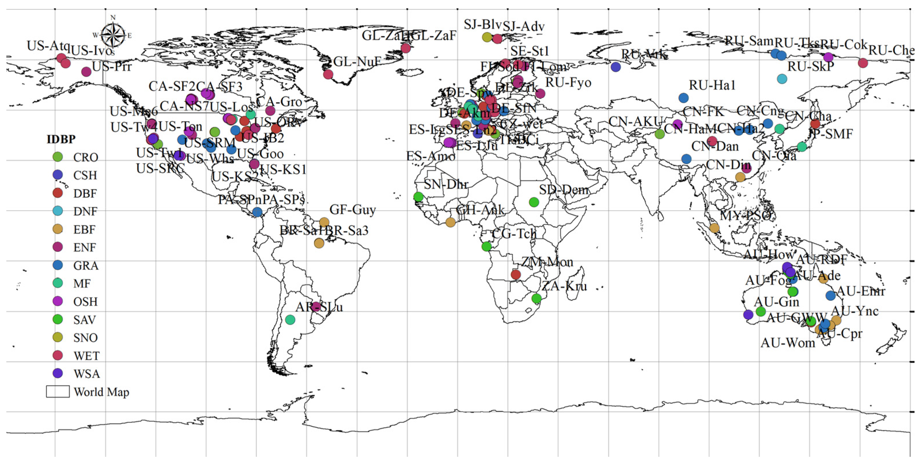
The latest FLUXNET dataset is the FLUXNET2015 dataset (http://fluxnet.fluxdata.org/, accessed on 12 October 2022), which includes annual data from 212 flux sites (Figure 2). Carbon, water, and heat fluxes for these sites are recorded in detail, with data durations ranging from one year to more than a decade. The flux sites consist of the following 13 types of sites, including 49 evergreen coniferous forest (ENF) sites, 15 evergreen broad-leaved forest (EBF) sites, 1 deciduous coniferous forest (DNF) site, 26 deciduous broad-leaved forest (DBF) sites, 9 mixed-forest (MF) sites, 3 closed-shrub forest (CSH) sites, 13 sparse-shrub forest (OSH) sites, 6 forest and grassland (WSA) sites, 9 savanna (SAV) sites, 39 grassland (GRA) sites, 20 permanent wetland (WET) sites, 19 farmland (CRO) sites, and 1 snow and ice (SNO) site.

4. Results and Analysis

4.1. Sensitivity Analysis of Numerical Calibration for End-Element Component Quantiles

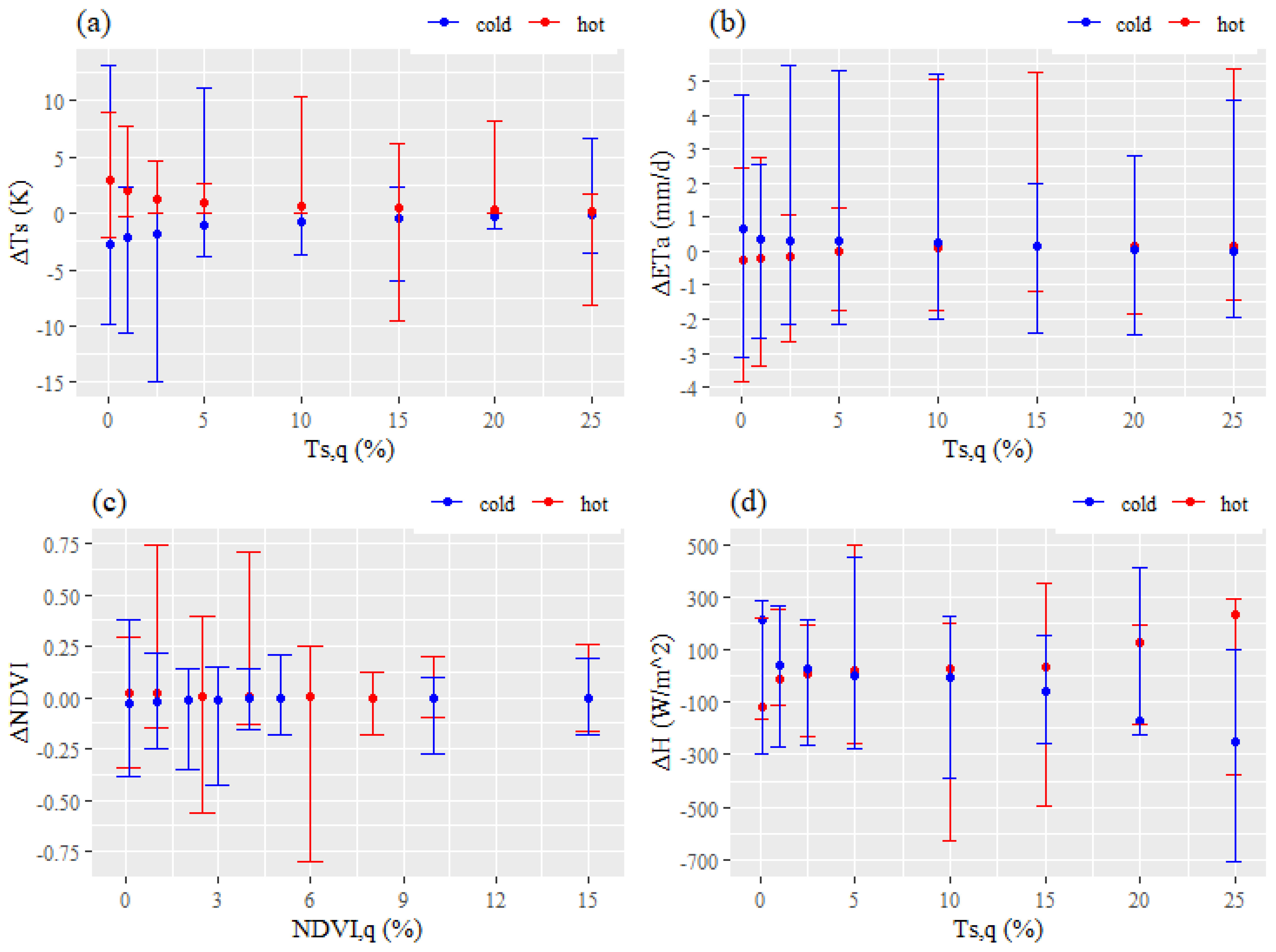
Figure 3 presents a sensitivity analysis of the endmember component percentile values q with respect to variations in ΔTs, ΔETa, ΔNDVI, and ΔH. As the Ts,q percentile values change from 0.01% to 25%, ΔTs, ΔETa, and ΔNDVI gradually approach zero, indicating that the influence of cold and hot pixels on these parameter values diminishes and stabilizes. For Ts, as the q value rises from 0.001% to 5%, the average range of change for ΔTs in cold and hot pixels is 1.73 K to 1.99 K, resulting in an average range of change for ETa in cold and hot pixels from 0.27 mm/d to 0.39 mm/d and an average range of change for H in cold and hot pixels from 142.23 W/m2 to 209.97 W/m2. However, for Ts,q > 5%, the change in Ts for cold and hot pixels is minor, less than 1 K, resulting in an average change in ETa for cold and hot pixels of less than 0.24 mm/d. When Ts,q < 5%, ΔH,cold > ΔH,hot; conversely, when Ts,q > 5%, ΔH,cold < ΔH,hot. The overall trend shows that as the Ts,q percentile value gradually increases from 0.01% to 25%, ΔH,cold gradually decreases, while ΔH,hot gradually increases. Additionally, the changes in ΔTs, ΔETa, ΔNDVI, and ΔH for cold and hot pixels are all symmetrically distributed around the zero value, showing a certain symmetry.
Regarding NDVI, with the change in percentile value q, the amplitude is relatively small, indicating the least sensitivity among the parameters. Laipelt et al. reached a similar conclusion through their research, finding that the sensitivity to Ts,q is higher than that of the percentile value NDVI,q [43]. From Figure 3, it can be inferred that H is the most sensitive to the percentile values of the endmember components. Long et al. suggested that an increase of 2 K in Ts,cold and Ts,hot would lead to an average decrease of 14.6% in the estimated value of H [31]. This is inconsistent with the findings of the present study, mainly because Long et al. only considered the results of ΔTs fluctuating within the range of −5 K to 5 K and neglected values below and above this range [27]. From Figure 3a, it is observed that the fluctuation amplitude of ΔTs is between −13.117 K and 14.93 K, indicating that values outside the threshold range would affect the results for H. The mean values of ΔTs and ΔNDVI for cold pixels increase with increasing q percentile values, while the trend for hot pixels is the opposite, as shown in Figure 3a,c. The trends for the mean values of ΔETa and ΔH in cold pixels are opposite to those of ΔTs and ΔNDVI, decreasing with the increasing q percentile value while they increase for hot pixels, as illustrated in Figure 3b,d. Kayser et al. also recognized that cold endmember components are more sensitive to parameter influences [44]. In conclusion, in most cases, the range of variation for cold pixels is larger than that for hot pixels, implying that the data for cold pixels are more unstable or are influenced by a greater number of factors.
Table 4 shows the evaluation of the quantile of the optimized endmember components (Ts,cold, Ts,hot, NDVI,cold, and NDVI,hot) under different vegetation types. The overall root mean square error (RMSE) ranges from 0.99 to 4.89, the bias ranges from −1.34 to 0.79, the Nash–Sutcliffe efficiency coefficient ranges from −2.16 to 0.67, and the correlation coefficient varies from 0.47 to 0.76. Laipelt et al. calibrated the percentile values for rainforests, grasslands, and farmlands, providing intervals for the endmember component percentiles, such as 0.01% to 1% for Ts,cold in rainforests, 0.01% to 10% for Ts,hot, 5% for NDVI,cold, and 1% to 10% for NDVI,hot [42]. Kayser et al. validated this for farmland under the subtropical humid climate in southern Brazil, finding percentile intervals with Ts,cold ranging from 0.01% to 25%, Ts,hot ranging from 0.01% to 25%, NDVI,cold at 5%, and NDVI,hot at 10% [44].

4.2. Sensitivity Analysis of Model Parameters

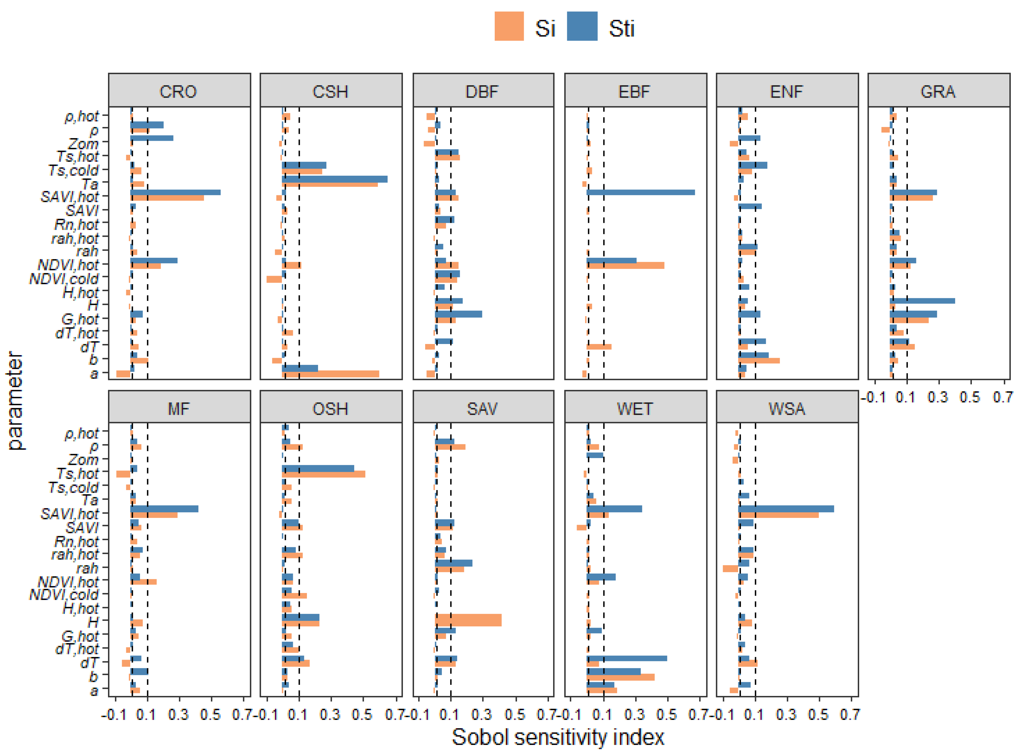
Through the analysis of parameter sensitivity across various vegetation types (Figure 4), it can be inferred that there exist substantial disparities in highly sensitive parameters (Sti > 0.1) among different vegetation types. The most sensitive parameter of CRO, EBF, MF, and WSA is SAVI,hot; Ts,cold is the most sensitive parameter of CSH. There is a relatively small difference between the parameters of DBF and ENF types, and the most sensitive parameters are G,hot and b, respectively. H is the most sensitive parameter for GRA and SAV types. Ts,hot is the most sensitive parameter of OSH, and dT is the most sensitive parameter of WET.
Through a sensitivity index ranking analysis of the 20 parameters of the geeSEBAL model, it was found that dT and SAVI,hot are highly sensitive parameters, with Sti values greater than 0.1, which have a significant impact on the output of the model’s ETa results. All the other parameters are sensitive, with Sti values ranging from 0.01 to 0.1. Specifically, Ts,hot, Ts,cold, NDVI,hot, NDVI,cold, SAVI, SAVI,hot, ρ, ρ,hot, Rn,hot, G,hot, H, Zom, rah, rah,hot, Ta, dT,hot, b, a, H,hot, and Zom are all classified as sensitive parameters (Figure 5). Among these sensitive parameters, the high-order Sti values of SAVI,hot and dT are 1.884 times and 2.545 times higher than the low-order Si values, respectively (Figure 5).

4.3. Optimization of the SEBAL Model Based on Measured ETa Data from Flux Stations

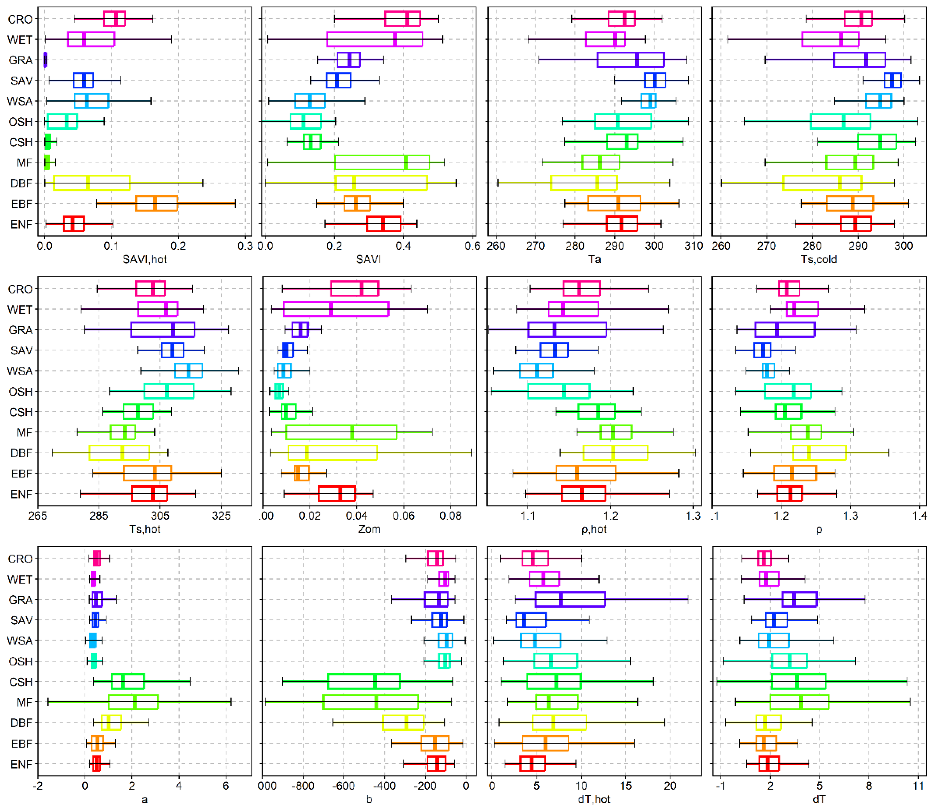
The posterior distributions of 20 parameters after sensitivity analysis by using the DE-MC method are shown in Figure 6, and the posterior distributions of all parameters showed significant fluctuations under various vegetation types. The difference in the ΔTs values of hot pixels is higher than that of cold pixels, and it is difficult to identify hot pixels because there are multiple pixels that meet the selection criteria. The parameters ρ,hot, dT,hot, and rah,hot showed relatively stable posterior distributions among the vegetation types (with distribution ranges of 1.11~1.21, 4.56 K~8.26 K, and 17.99~35.97). The original value of the parameter Zom is usually 0.005 m [45]. After optimization, the Zom values of ENF, EBF, DBF, and MF, which are mainly forest systems, are relatively high, ranging from 0.015 m to 0.039 m. The values of Zom in non-forest ecosystems (including GRA, SAV, WSA, OSH and CSH, except CRO and WET) are lower, ranging from 0.0069 m to 0.016 m. The size distribution trends of a and b are opposite. The median value of the parameter a of CSH, MF, and DBF is significantly higher than that of other land cover types, while the parameter b is the opposite (Figure 6). Except for GRA, SAV, and WSA, Ta shows high values (Ta > 295 K), and the posterior distributions of Ta among the other land cover types are relatively stable (for most of them, Ta < 292 K). The median values of H are higher in CSH and MF (H > 270 W/m2), while the values of H in other land cover types are all at a low value (H < 120 W/m2).
Table 5 provides the evaluation results of the SEBAL model before and after optimization; the overall evaluation results of the optimized model are higher than those of the original model. The land cover type is the most sensitive factor affecting the parameters of the SEBAL model. The ENF, EBF, DBF, CSH, and OSH optimization algorithms underestimated ETa (bias < 0), while the MF, WSA, SAV, GRA, WET, and CRO optimization algorithms overestimated ETa (bias > 0) (Table 5).

5. Discussion

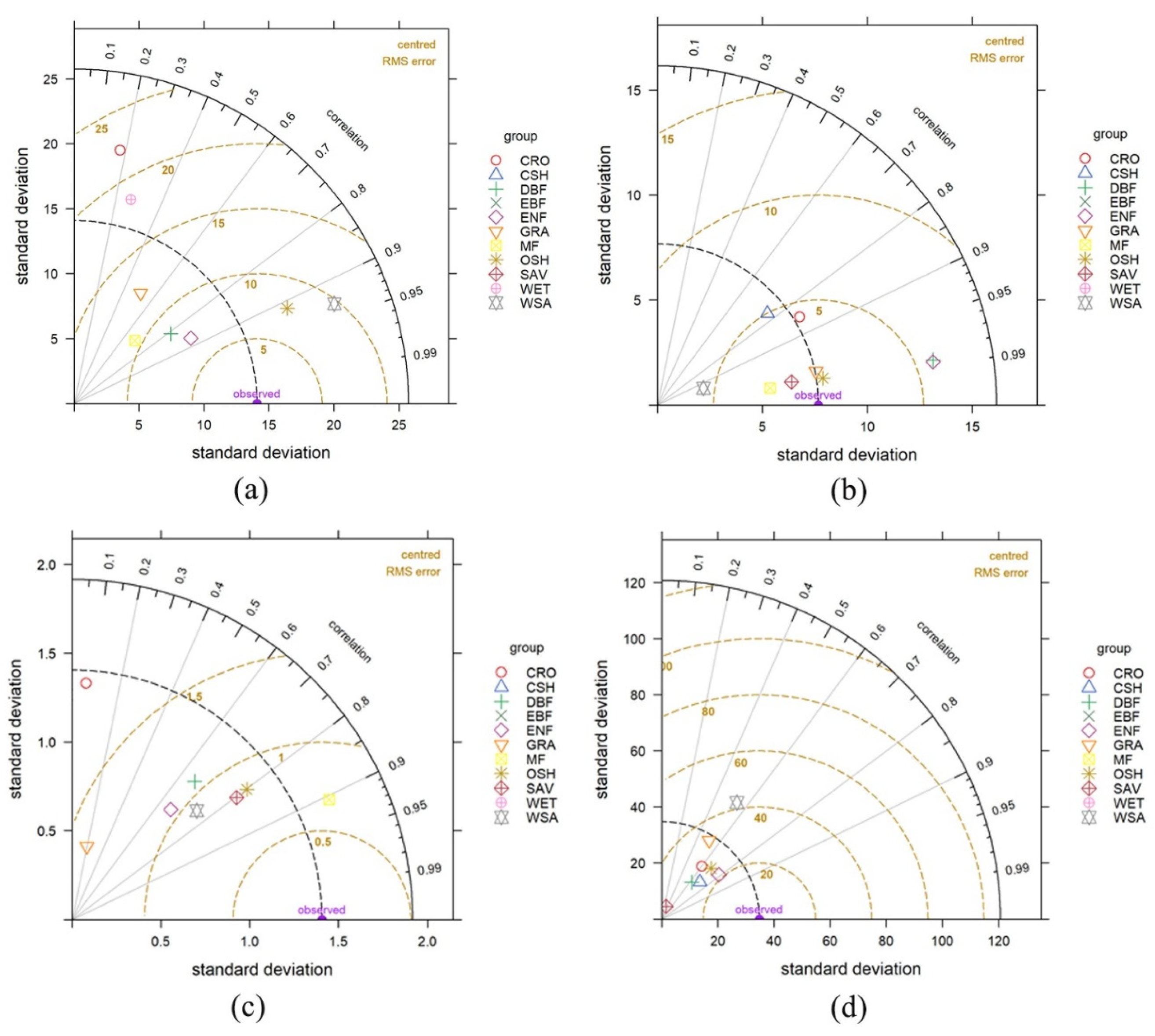
Figure 7 shows the standard deviation on the axis of the Taylor plot. The black curve represents the correlation coefficient, and the yellow dashed curve represents the centered root mean square error (RMSE). The relative humidity RH and wind speed WS show significant fluctuations, with correlation coefficients ranging from 0.05 to 0.95, and the CRO effect is the worst (Figure 7a,c). This is similar to the conclusion of Qi et al. in evaluating GLDAS meteorological data, which suggests that there is an overestimation of WS and that the variable needs to be adjusted by a coefficient of 0.76 [44]. However, Kayser et al. found that the wind speed correction coefficient should be 0.71, and the estimation effect of RH is poor [45]. The effect of T is the best, with the highest correlation coefficient of T reaching 0.99 (including OSH, SAV, and MF) and the lowest exceeding 0.78 (CSH) (Figure 7b). The correlation coefficient of Rn ranges from 0.55 to 0.8 (Figure 7d). From this, it can be concluded that the uncertainty of the ERA5 dataset in the geeSEBAL model is an important factor that cannot be ignored. Optimizing and adjusting these data can greatly improve the simulation accuracy of the model.

6. Conclusions

In this study, optimizing the quantile values of the reverse-modelling automatic calibration algorithm (CIMEC) endpoint-component selection algorithm under extreme conditions was found to be a necessary step for the geeSEBAL algorithm to estimate ETa. We optimized the quantile values of the end element components by setting endpoint calibration scenarios and using measured data from 212 global flux stations, and the optimized results were satisfactory. We applied the Sobol method to identify sensitive parameters of the geeSEBAL algorithm. Under different vegetation types, the highly sensitive parameters of simulated evaporation are dT and SAVI,hot. For different biological communities, the sensitive parameters may change. Therefore, when using high-resolution remote-sensing data for ETa estimation, it is necessary to optimize each vegetation type separately. For example, the ENF (forestland) coverage type has seven highly sensitive parameters (SAVI, Ts,cold, G,hot, Zom, rah, b, and dT). Most of the key parameters are related to thermal pixels, and these parameterization schemes significantly affect the accuracy of the simulation. It should be pointed out that for all biological communities, the geeSEBAL algorithm has the highest sensitivity to SAVI,hot, and in the original model, this parameter is usually not taken into account. We optimized 20 parameters of geeSEBAL using the DE-MC method based on data from 212 global flux observation stations. The posterior distribution of the selected parameters was successfully limited by these observations (i.e., it showed a narrower range of variation distribution than the original geeSEBAL). Through model evaluation, the optimized algorithm performs better than the original algorithm. Nevertheless, even after quantile and parameter optimization, the geeSEBAL algorithm still has certain shortcomings in specific situations. The uncertainty of the predefined parameter Zoh and the reanalysis of meteorological parameter inputs are also reasons for this. It may also be related to errors in the model structure and the uncertainty of the mandatory data. The geeSEBAL algorithm is based on an energy balance model that lacks consideration of water, such as soil evaporation and vegetation transpiration. In addition, with the increase in in situ flux data and other available observation data, the parameters of the geeSEBAL algorithm should be further optimized to further improve the accuracy of the simulation.

Author Contributions

Conceptualization, P.J., C.T. and S.H.; methodology, P.J.; software, P.J.; validation, P.J.; formal analysis, P.J.; investigation, P.J. and S.H.; resources, S.H.; data curation, P.J., C.T. and S.H.; writing—original draft preparation, P.J.; writing—review and editing, P.J. and S.H.; supervision, C.T. and S.H. All authors have read and agreed to the published version of the manuscript.

Funding

This research was funded by the special fund project of the National Key R&D Program of China (No. 2021YFD1900801), the National Natural Science Foundation of China (No. 41671032), and the Xinjiang Water Conservancy Science and Technology (No. YF2020-08 and XSKJ-2021-05).

Data Availability Statement

Data are contained within the article.

Conflicts of Interest

The authors declare no conflicts of interest.

References

  1. Maroufpoor, S.; Bozorg-Haddad, O.; Maroufpoor, E. Reference evapotranspiration estimating based on optimal input combination and hybrid artificial intelligent model: Hybridization of artificial neural network with grey wolf optimizer algorithm. J. Hydrol. 2020, 588, 125060. [Google Scholar] [CrossRef]
  2. Vinukollu, R.K.; Wood, E.F.; Ferguson, C.R.; Fisher, J.B. Global estimates of evapotranspiration for climate studies using multi-sensor remote sensing data: Evaluation of three process-based approaches. Remote Sens. Environ. 2011, 115, 801–823. [Google Scholar] [CrossRef]
  3. Chao, L.; Zhang, K.; Wang, J.; Feng, J.; Zhang, M. A comprehensive evaluation of five evapotranspiration datasets based on ground and GRACE satellite observations: Implications for improvement of evapotranspiration retrieval algorithm. Remote Sens. 2021, 13, 2414. [Google Scholar] [CrossRef]
  4. Novick, K.A.; Ficklin, D.L.; Stoy, P.C.; Williams, C.A.; Bohrer, G.; Oishi, A.C.; Papuga, S.A.; Blanken, P.D.; Noormets, A.; Sulman, B.N.; et al. The increasing importance of atmospheric demand for ecosystem water and carbon fluxes. Nat. Clim. Chang. 2016, 6, 1023–1027. [Google Scholar] [CrossRef]
  5. Talebmorad, H.; Abedi-Koupai, J.; Eslamian, S.; Mousavi, S.F.; Akhavan, S.; Ostad-Ali-Askari, K.; Singh, V.P. Evaluation of the impact of climate change on reference crop evapotranspiration in Hamedan-Bahar plain. Int. J. Hydrol. Sci. Technol. 2021, 11, 333–347. [Google Scholar] [CrossRef]
  6. Anderson, M.C.; Hain, C.; Otkin, J.; Zhan, X.; Mo, K.; Svoboda, M.; Wardlow, B.; Pimstein, A. An intercomparison of drought indicators based on thermal remote sensing and NLDAS-2 simulations with U.S. drought monitor classifications. J. Hydrometeorol. 2013, 14, 1035–1056. [Google Scholar] [CrossRef]
  7. Schwalm, C.R.; Huntinzger, D.N.; Michalak, A.M.; Fisher, J.B.; Kimball, J.S.; Mueller, B.; Zhang, K.; Zhang, Y. Sensitivity of inferred climate model skill to evaluation decisions: A case study using CMIP5 evapotranspiration. Environ. Res. Lett. 2013, 8, 024028. [Google Scholar] [CrossRef]
  8. Wang, S.; Pan, M.; Mu, Q.; Shi, X.; Mao, J.; Brümmer, C.; Jassal, R.S.; Krishnan, P.; Li, J.; Black, T.A. Comparing evapotranspiration from eddy covariance measurements, water budgets, remote sensing, and land surface models over Canada. J. Hydrometeorol. 2015, 16, 1540–1560. [Google Scholar] [CrossRef]
  9. Kim, Y.; Kimball, J.S.; Zhang, K.; Didan, K.; Velicogna, I.; McDonald, K.C. Attribution of divergent northern vegetation growth responses to lengthening nonfrozen seasons using satellite optical-NIR and microwave remote sensing. Int. J. Remote Sens. 2014, 35, 3700–3721. [Google Scholar] [CrossRef]
  10. Zhao, L.; Xia, J.; Xu, C.Y.; Wang, Z.; Sobkowiak, L.; Long, C. Evapotranspiration estimation methods in hydrological models. J. Geog. Sci. 2013, 23, 359–369. [Google Scholar] [CrossRef]
  11. Huntingford, C.; Verhoef, A.; Stewart, H. Dual versus single source models for estimating surface temperature of African savannah. Hydrol. Earth Syst. Sci. 2000, 4, 185–191. [Google Scholar] [CrossRef]
  12. Lhomme, J.P.; Monteney, B.; Amadou, M. Estimating sensible heat flux from radiometric temperature over sparse millet. Agric. Water Manag. 1994, 68, 77–91. [Google Scholar] [CrossRef]
  13. Bastiaanssen, W.G.M. SEBAL-based sensible and latent heat fluxes in the irrigated Gediz Basin. Turkey J. Hydrol. 2000, 229, 87–100. [Google Scholar] [CrossRef]
  14. Allen, R.G.; Tasumi, M.; Morse, A. Satellite-based evapotranspiration by METRIC and Landsat for western states water management. In Proceedings of the U.S. Bureau of Reclamation Evapotranspiration Workshop, Ft. Collins, CO, USA, 8–10 February 2005. [Google Scholar]
  15. Allen, R.G.; Tasumi, M.; Trezza, R. Satellite-based energy balance for mapping evapotranspiration with internalized calibration (METRIC)—Model. J. Irrig. Drain. Eng. 2007, 133, 380–394. [Google Scholar] [CrossRef]
  16. Su, Z.; Schmugge, T.; Kustas, W.P.; Massman, W.J. An evaluation of two models for estimation of the roughness height for heat transfer between the land surface and the atmosphere. J. Appl. Meteorol. 2001, 40, 1933–1951. [Google Scholar] [CrossRef]
  17. Su, Z.B. The surface energy balance system (SEBS) for estimation of turbulent heat fluxes. Hydrol. Earth Syst. Sci. 2002, 6, 85–99. [Google Scholar] [CrossRef]
  18. Jaafar, H.; Mourad, R.; Schull, M. A global 30-m ET model (HSEB) using harmonized Landsat and Sentinel-2, MODIS and VIIRS: Comparison to ECOSTRESS ET and LST. Remote Sens. Environ. 2022, 274, 112995. [Google Scholar] [CrossRef]
  19. Senay, G.B.; Budde, M.; Verdin, J.P.; Melesse, A.M. A coupled remote sensing and simplified surface energy balance approach to estimate actual evapotranspiration from irrigated fields. Sensors 2007, 7, 979–1000. [Google Scholar] [CrossRef]
  20. Anderson, M.C.; Kustas, W.P.; Norman, J.M.; Hain, C.R.; Mecikalski, J.R.; Schultz, L.; Gonzalez-Dugo, M.P.; Cammalleri, C.; d’Urso, G.; Pimstein, A.; et al. Mapping daily evapotranspiration at field to continental scales using geostationary and polar orbiting satellite imagery. Hydrol. Earth Syst. Sci. 2011, 15, 223–239. [Google Scholar] [CrossRef]
  21. Marshall, M.; Tu, K.; Andreo, V. On parameterizing soil evaporation in a direct remote sensing model of ET: PT—JPL. Water Resour. Res. 2020, 56, e2019WR026290. [Google Scholar] [CrossRef]
  22. Mu, Q.; Heinsch, F.A.; Zhao, M.; Running, S.W. Development of a global evapotranspiration algorithm based on modis and global meteorology data. Remote Sens. Environ. 2007, 111, 519–536. [Google Scholar] [CrossRef]
  23. Mu, Q.; Zhao, M.; Running, S.W. Running. Improvements to a modis global terrestrial evapotranspiration algorithm. Remote Sens. Environ. 2011, 115, 1781–1800. [Google Scholar] [CrossRef]
  24. Mu, Q.; Zhao, M.; Kimball, J.S.; McDowell, N.G.; Running, S.W. A remotely sensed global terrestrial drought severity index. Am. Meteorol. Soc. 2013, 94, 83–98. [Google Scholar] [CrossRef]
  25. Zhao, F.; Ma, S.; Wu, Y.; Qiu, L.; Wang, W.; Lian, Y.; Chen, J.; Sivakumar, B. The role of climate change and vegetation greening on evapotranspiration variation in the Yellow River Basin, China. Agric. For. Meteorol. 2022, 316, 108842. [Google Scholar] [CrossRef]
  26. Veloso, G.A.; Ferreira, M.E.; Júnior, L.G.F.; da Silva, B.B. Modelling gross primary productivity in tropical savanna pasturelands for livestock intensification in Brazil. Remote Sens. Appl. Soc. Environ. 2020, 17, 100288. [Google Scholar] [CrossRef]
  27. Long, D.; Singh, V.P. Assessing the impact of end-member selection on the accuracy of satellite-based spatial variability models for actual evapotranspiration estimation. Water Resour. Res. 2013, 49, 2601–2618. [Google Scholar] [CrossRef]
  28. Hong, S.; Hendrickx, J.M.H.; Borchers, B. Up-scaling of SEBAL derived evapotranspiration maps from Landsat (30 m) to MODIS (250 m) scale. J. Hydrol. 2009, 370, 122–138. [Google Scholar] [CrossRef]
  29. Bhattarai, N.; Liu, T. LandMOD ET mapper: A new matlab-based graphical user interface (GUI) for automated implementation of SEBAL and METRIC models in thermal imagery. Environ. Model. Softw. 2019, 118, 76–82. [Google Scholar] [CrossRef]
  30. Morton, C.G.; Huntington, J.L.; Pohll, G.M.; Allen, R.G.; McGwire, K.C.; Bassett, S.D. Assessing calibration uncertainty and automation for estimating evapotranspiration from agricultural areas using METRIC. J. Am. Water Resour. Assoc. 2013, 49, 549–562. [Google Scholar] [CrossRef]
  31. Long, D.; Singh, V.P.; Li, Z.L. How sensitive is SEBAL to changes in input variables, domain size and satellite sensor? J. Geophys. Res. 2011, 116, 1–20. [Google Scholar] [CrossRef]
  32. Marx, A.; Kunstmann, H.; Schüttemeyer, D.; Moene, A.F. Uncertainty analysis for satellite derived sensible heat fluxes and scintillometer measurements over Savannah environment and comparison to mesoscale meteorological simulation results. Agric. For. Meteorol. 2008, 148, 656–667. [Google Scholar] [CrossRef]
  33. Allen, R.G.; Burnett, B.; Kramber, W.; Huntington, J.; Kjaersgaard, J.; Kilic, A.; Kelly, C.; Trezza, R. Automated calibraton of the METRIC-Landsat evapotranspiration process. J. Am. Water Resour. Assoc. 2013, 49, 563–576. [Google Scholar] [CrossRef]
  34. Wang, J.; Sammis, T.W.; Gutschick, V.P.; Gebremichael, M.; Miller, D.R. Sensitivity Analysis of the Surface Energy Balance Algorithm for Land (SEBAL). Trans. ASABE 2009, 52, 801–811. [Google Scholar] [CrossRef]
  35. Sobol’, I.M. Global sensitivity indices for nonlinear mathematical models and their Monte Carlo estimates. Math. Comput. Simul 2001, 55, 271–280. [Google Scholar] [CrossRef]
  36. Brust, C.; Kimball, J.S.; Maneta, M.P.; Jencso, K.; He, M.; Reichle, R.H. Using SMAP Level-4 soil moisture to constrain MOD16 evapotranspiration over the contiguous USA. Remote Sens. Environ. 2021, 255, 112277. [Google Scholar] [CrossRef]
  37. Clark, J.S.; Gelfand, A.E. A future for models and data in environmental science. Trends Ecol. Evol. 2006, 21, 375–380. [Google Scholar] [CrossRef]
  38. Vrugt, J.A.; ter Braak, C.J.; Diks, C.G.; Robinson, B.A.; Hyman, J.M.; Higdon, D. Accelerating Markov chain Monte Carlo simulation by differential evolution with self-adaptive randomized subspace sampling. Int. J. Nonlinear Sci. Numer. Simul. 2009, 10, 273–290. [Google Scholar] [CrossRef]
  39. Ter Braak, C.J.; Vrugt, J.A. Differential evolution Markov chain with snooker updater and fewer chains. Stat. Comput. 2008, 18, 435–446. [Google Scholar] [CrossRef]
  40. Bastiaanssen, W.G.M.; Menenti, M.; Feddes, R.A.; Holtslag, A.A.M. The surface energy balance algorithm for land (SEBAL): Part 1 formulation. J. Hydrol. 1998, 212–213, 198–212. [Google Scholar] [CrossRef]
  41. Bastiaanssen, W.G.M.; Menenti, M.; Feddes, R.A.; Holtslag, A.A.M. A remote sensing surface energy balance algorithm for land (SEBAL) 1. formulation. J. Hydrol. 1998, 212–213, 213–229. [Google Scholar] [CrossRef]
  42. Laipelt, L.; Kayser, R.H.B.; Fleischmann, A.S.; Ruhoff, A.; Bastiaanssen, W.; Erickson, T.A.; Melton, F. Long-term monitoring of evapotranspiration using the SEBAL algorithm and Google Earth Engine cloud computing. ISPRS J. Photogramm. Remote Sens. 2021, 178, 81–96. [Google Scholar] [CrossRef]
  43. Laipelt, L.; Ruhoff, A.L.; Fleischmann, A.S.; Kayser, R.H.B.; Kich, E.D.M.; da Rocha, H.R.; Neale, C.M.U. Assessment of an automated calibration of the SEBAL algorithm to estimate dry-season surface-energy partitioning in a Forest—Savanna transition in Brazil. Remote Sens. 2020, 12, 1108. [Google Scholar] [CrossRef]
  44. Kayser, R.H.; Ruhoff, A.; Laipelt, L.; de Mello Kich, E.; Roberti, D.R.; de Arruda Souza, V.; Rubert, G.C.D.; Collischonn, W.; Neale, C.M.U. Assessing geeSEBAL automated calibration and meteorological reanalysis uncertainties to estimate evapotranspiration in subtropical humid climates. Agric. For. Meteorol. 2022, 314, 108775. [Google Scholar] [CrossRef]
  45. Nishida, K.; Nemani, R.R.; Running, S.W.; Glassy, J.M. An operational remote sensing algorithm of land surface evaporation. J. Geophys. Res. 2003, 108, D94270. [Google Scholar] [CrossRef]
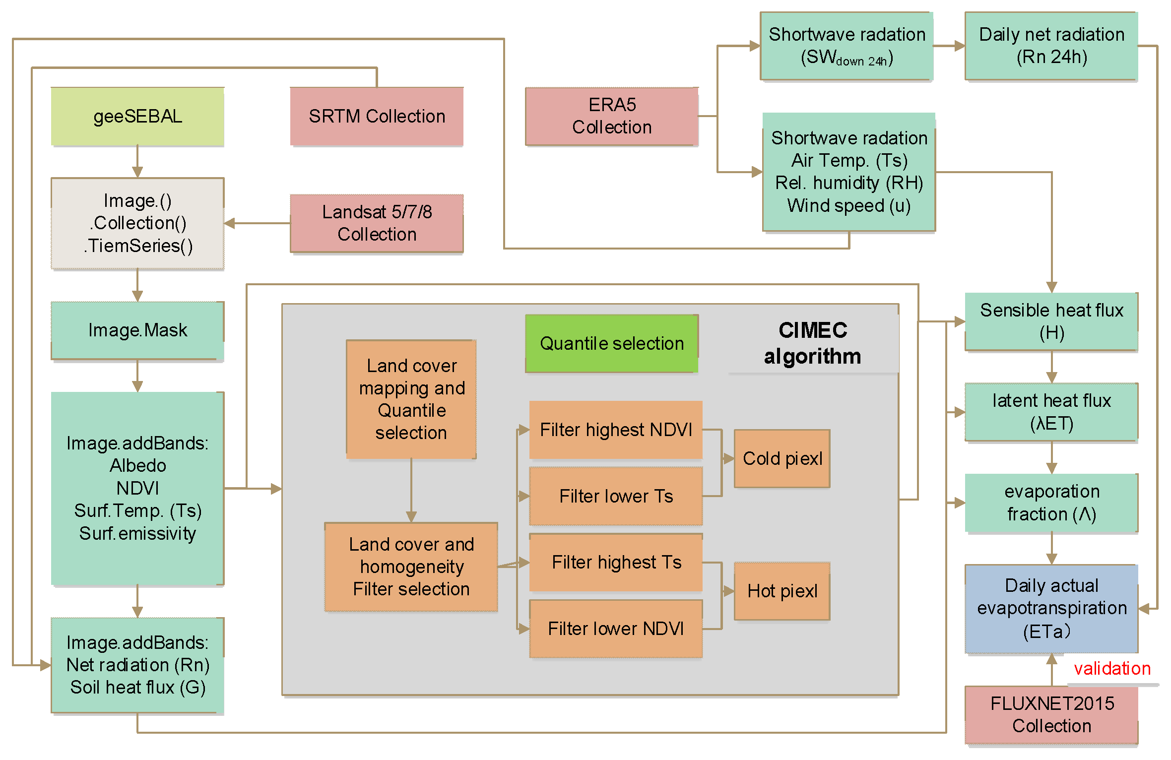
Figure 1. Framework diagram of geeSEBAL model based on the CIMEC algorithm.
Water 16 02978 g001
Figure 2. Spatial distribution of available global flux sites in the FLUXNET2015 dataset (review number: GS (2021) 6375).
Water 16 02978 g002
Figure 3. Changes in the quantile value q of end-element components on cold and hot pixels ΔTs, ΔETa, ΔNDVI, and ΔH sensitivity: the high and low lines in the graph represent the maximum and minimum changes, and the points represent the average changes. (a) ΔTTs,q, (b) ΔETaTs,q, (c) ΔNDVINDVI,q and (d) ΔHTs,q.
Water 16 02978 g003
Figure 4. Sensitivity of the Sobol first-order and total-order parameters for different vegetation types.
Water 16 02978 g004
Figure 5. First-order (Si) (a) and full-order (Sti) (b) sensitivity analyses of the SEBAL model parameters based on Sobol’s method. The red dotted line and the black dotted line represent 0.1 and 0, respectively, and the parameters above the red dashed line are extremely sensitive parameters, and the parameters above the black dashed line are sensitive parameters.
Water 16 02978 g005
Figure 6. Posterior distribution of the geeSEBAL model parameters for various vegetation types.
Water 16 02978 g006aWater 16 02978 g006b
Figure 7. ERA5 Meteorological input evaluation station verification Taylor chart relative humidity RH (a), temperature T (b), wind speed WS (c), and net radiation Rn (d).
Water 16 02978 g007
Table 1. SEBAL model parameterization scheme and Bayesian prior distribution.
ParametersDescribeIntermediate VariablePrior DistributionUnit
Ts,hotMaximum surface temperature Ts in pixels a , b d T H λ E T [280.16, 320.84]K
Ts,coldMinimum value of surface temperature Ts in pixels a , b d T H λ E T [267.50, 302.44]K
NDVI,hotCompletely exposed surface NDVI value a , b d T H λ E T [0.12, 0.28]-
NDVI,coldSurface NDVI values completely covered by vegetation a , b d T H λ E T [0.79, 0.81]-
SAVIAdjusting the vegetation index for soil brightness Z o m r a h H λ E T [−1, 1]-
SAVI,hotVegetation index for adjusting soil brightness limited by maximum surface temperature Ts Z o m r a h H λ E T [0, 0.285]-
ρair density H λ E T [1.134, 1.356]kg/m3
ρ,hotThermal pixel air density a , b d T H λ E T [1.061, 1.179]kg/m3
Rn,hotThermal pixel net radiation a , b d T H λ E T [0, 250]W/m2
G,hotThermal image element soil heat flux a , b d T H λ E T [125.1, 188.5]W/m2
HSensible heat flux λ E T [101, 239.9]W/m2
H,hotThermal pixel sensible heat flux H λ E T [48.089, 716.254]W/m2
ZomSurface roughness r a h H λ E T [0.015, 0.1]m
rahAerodynamic impedance between different heights of land surface H λ E T [5.168, 136.415]-
rah,hotAerodynamic impedance between land surface at different heights limited by maximum surface temperature Ts a , b d T H λ E T [0.0117, 103.761]-
TaSurface temperature per pixel d T H λ E T ;
G λ E T
[260.536, 308.668]K
dTTemperature difference between different heights of land surface H λ E T [−1.26, 10.431]K
dT,hotTemperature difference between different heights of land surface limited by maximum surface temperature Ts H λ E T [0.119, 22.014]K
aRegression coefficient of cold and hot pixels d T H λ E T [0.22, 1.22]-
bRegression coefficient of cold and hot pixels d T H λ E T [−367.3, −63.6]-
Table 2. Endpoint calibration scenario setting.
PixelEnd Element ComponentsQuantiles
Cold (wet)NDVI0.01%, 0.1%, 1%, 2%, 3%, 4%, 5%,10%,15%.
Ts0.01%, 0.1%, 1%, 2.5%, 5%, 10%, 15%, 20%, 25%.
Hot (dry)NDVI0.01%, 0.1%, 1%, 2.5%, 4%, 6%, 8%, 10%,15%.
Ts0.01%, 0.1%, 1%, 2.5%, 5%, 10%, 15%, 20%, 25%.
Table 3. Description of available sets for the geeSEBAL algorithm.
ProductGEE IDBandTime FrameResolution Ratio
LANDSAT 5 TMLANDSAT/LT05/C01/T1_SR LANDSAT/LT05/C01/T1Surface reflectance, brightness temperature, pixel QA (quality attributes)1984–201230 m
LANDSAT 7 ETM+LANDSAT/LE07/C01/T1_SRLANDSAT/LE07/C01/T1Surface reflectance, brightness temperature, pixel QA (quality attributes)1999–Now30 m
LANDSAT 8 OLI/TIRSANDSAT/LC08/C01/T1_SRLANDSAT/
LC08/C01/T1
Surface reflectance, brightness temperature, pixel QA (quality attributes)2013–Now30 m
ERA5-Land hourlyECMWF/ERA5_LAND/HOURLYAir temperature at 2 m, dew point temperature at 2 m, eastward wind speed at 10 m, northward wind speed at 10 m, surface solar radiation.1981–Now0.1°
SRTMUSGS/SRTMGL1_003Elevation200030 m
Table 4. Optimal quantile for selecting the end-element components of different vegetation types.
TypeEnd Element Component QuantilesEffects
Ts,cold (K)Ts,hot (K)NDVI,coldNDVI,hotRMSE (mm/d)Bias (mm/d)NSER2
ENF110162.31−0.38−0.930.64
EBF252515152.11−0.31−0.780.52
DBF5253151.890.050.670.76
MF0.1100.162.670.090.340.61
CSH2.5252152.45−1.34−0.570.51
OSH100.140.14.89−1.09−1.890.47
WSA250.01150.010.99−0.89−2.160.53
SAV0.1250.1152.110.56−0.040.54
GRA0.01100.0163.670.79−0.450.53
WET150.0150.012.76−0.890.130.66
CRO20205101.25−0.06−0.890.77
Table 5. Evaluation of the geeSEBAL model before and after optimization.
Type RMSE (mm/d)Bias (mm/d)NSER2
ENFOri7.67−3.14−0.450.55
Opt2.16−1.780.530.65
EBFOri5.34−2.11−0.730.57
Opt1.42−0.750.350.63
DBFOri8.180.190.340.49
Opt0.66−0.110.520.6
MFOri4.591.550.540.52
Opt1.361.010.650.63
CSHOri2.88−3.51−0.170.6
Opt0.08−1.350.120.67
OSHOri3.23−2.57−1.040.47
Opt1.02−1.760.150.53
WSAOri6.45−1.760.340.53
Opt2.321.130.550.59
SAVOri4.194.1−4.670.41
Opt1.672.59−0.270.45
GRAOri2.11−1.05−1.40.51
Opt0.450.980.110.59
WETOri7.981.80.130.55
Opt2.051.430.470.69
CROOri6.121.80.060.62
Opt1.241.020.570.73
Disclaimer/Publisher’s Note: The statements, opinions and data contained in all publications are solely those of the individual author(s) and contributor(s) and not of MDPI and/or the editor(s). MDPI and/or the editor(s) disclaim responsibility for any injury to people or property resulting from any ideas, methods, instructions or products referred to in the content.