Article

Inversion Method for Material Parameters of Concrete Dams Using Intelligent Algorithm-Based Displacement Separation

1
Powerchina Huadong Engineering Corporation Limited, Hangzhou 311122, China
2
College of Water Conservancy and Hydropower Engineering, Hohai University, Nanjing 210098, China
*
Authors to whom correspondence should be addressed.
Water 2024, 16(20), 2979; https://doi.org/10.3390/w16202979
Submission received: 20 September 2024 / Revised: 10 October 2024 / Accepted: 14 October 2024 / Published: 18 October 2024

Abstract

:
Integrating long-term observational data analysis with numerical simulations of dam operations provides an effective approach to dam safety evaluation. However, analytical results are often subject to errors due to challenges in accurately surveying and modeling the foundation, as well as temporal changes in foundation properties. This paper proposes a concrete dam displacement separation model that distinguishes between deformation caused by foundation restraint and that induced by external loads. By combining this model with intelligent optimization techniques and long-term observational data, we can identify the actual mechanical parameters of the dam and conduct structural health assessments. The proposed model accommodates multiple degrees of freedom and is applicable to both two- and three-dimensional dam modeling. Consequently, it is well-suited for parameter identification and health diagnosis of concrete gravity and arch dams with extensive observational data. The efficacy of this diagnostic model has been validated through computational case studies and practical engineering applications.

1. Introduction

Reservoirs have important functions such as flood control, water storage, irrigation, power generation, and shipping [1]. Concrete dams are a very important type of dam, which rely on the interaction between concrete and foundations to block upstream water and form a reservoir [2]. Concrete dams mainly include gravity dams and arch dams. The gravity dam mainly relies on the gravity of the concrete material to transfer the upstream water load to the foundation [3,4]. The arch dam mainly relies on the principle of arches and the compressive performance of concrete to transfer the water thrust to the abutments on both banks [5,6,7]. The stable and healthy operation of the dam–foundation system is of great significance in ensuring the safety of the reservoir controlled area [8,9]. As more and more concrete dams are built and put into use all over the world, the question of how to make accurate and efficient health diagnoses of concrete dams in long-term service has become a problem worthy of study [10]. The dam and foundation constitute a complex system with imbalance and uncertainty. Therefore, it is an important task to analyse the performance of the dam–foundation system based on the observation data during the operation, and infer its operation status [11].
For a concrete dam in operation, its long-term observation data is an essential part of the health diagnosis [12,13]. There are two main approaches to analyse dams based on observed data. One is ann analysis based on mathematical statistics [14,15]. A statistical model is established to describe the relationship between the external input and the internal responses [16,17]. Mata et al. [18] applied a hydrostatic, thermal, time (HTT) statistical model to the Alto Lindoso arch dam based on principal component analysis. Some researchers have used machine learning tools to establish this relationship [19]. Kang et al. [20] proposed an extreme learning machine (ELM)-based health monitoring model for displacement prediction of gravity dams. Dai et al. [21] used statistical models and random forest regression (RFR) models to predict concrete dam deformation. Kang et al. [22] used machine learning techniques to mine temperature effects in dam operation and validated the proposed dam health monitoring model using monitoring data from a real concrete gravity dam. From a mechanical point of view, means based purely on mathematical statistics lack a clear physical meaning, whereas the operation of a dam–foundation is a mechanical act.
The other approach is to establish a discrete numerical model based on mechanical principles, and use the numerical method to solve the response of the structures [23]. The obtained responses are compared with the observed data to determine whether the dam is operating normally. Bonaldi et al. [24] used a deterministic model incorporating finite element methods to analyse the safety of the dam. The simulation of structures by numerical methods requires accurate parameters [25], which are usually obtained during the engineering survey and design phase. After the concrete dam has been poured, the interior of the structure is largely unknown [26]. Field tests such as borehole sampling can be used to deduce the true state of the structure in part, but a complete identification of the system is not possible [27]. Using the output of deformation and strain and stress data measured by existing monitoring instruments to derive material parameters, boundary conditions, geometry, etc., in dam systems is an inverse problem in dam engineering research [28,29,30,31]. Yang et al. [32] used an improved particle swarm algorithm to optimise Young’s modulus of concrete dams and foundations. Kang et al. [6] used a machine learning-based response surface approach to invert the Young’s modulus of concrete arch dams. Lin et al. [33] proposed the identification of viscoelastic parameters of the foundation of a concrete gravity dam using the grey wolf optimisation algorithm and a non-linear finite element method.
The inversion of parameters plays a crucial role in the health diagnosis of dams. It allows engineers to obtain up-to-date information about the dam’s material properties and structural behavior, which may have changed over time due to various factors such as aging, environmental conditions, and loading history. By accurately determining these parameters, it becomes possible to assess the current state of the dam, predict its future performance, and make informed decisions about maintenance, repair, or rehabilitation strategies [34,35]. Furthermore, inverted parameters can be used to calibrate and validate numerical models, enhancing their reliability in simulating the dam’s response to various loading conditions and potential failure scenarios [36]. This process ultimately contributes to improved safety assessments, more efficient operation, and an extended service life of the dam structure.
Typically, a calculation area can be divided into several zones depending on the material ontology. However, it is inefficient or inaccurate to carry out an inverse analysis of the material parameters for all zones when almost all of them are uncertain, especially if the foundations are only roughly partitioned or directly replaced by a composite foundation [11]. On the other hand, when the foundations are too complex, a large number of finite element meshes are required to model them. Parametric optimisation is an expensive computational process that consumes a lot of resources. Too many finite element meshes can cause excessive use of computer memory and a reduction in solution speed [37,38]. It is worth investigating how to optimise the modelling of foundations and reduce the impact of foundation uncertainty. Lin et al. [39] proposed a dam form-core displacement separation model for a typical section of a gravity dam based on the framework of PFE-IE [40,41,42,43]. However, this method can only solve for three degrees of freedom and can therefore only be applied to the displacement separation of two-dimensional gravity dam cross-sections, and cannot be used to analyse concrete arch dam models that are in a three-dimensional state of stress. In addition, only the rigid displacement at the center of the dam can be solved for in the case of displacement separation.
In this paper, a new displacement separation method is proposed that allows the foundation restraint displacements of concrete dams to be separated out. The method is applicable to problems with different numbers of degrees of freedom and enables the numerical separation of the entire displacement field. The deformation of a concrete dam is separated into a part caused by foundation constraints and a part caused by external loads. To enable better application of the observations to the finite element model and to avoid increasing the complexity of the finite element model due to the location of the observation points, isoparametric cell displacement field interpolation methods based on shape functions are applied. When considering temperature effects [44,45], the temperature load is equated to a nodal force load. The validity of the separation method is verified using two case studies. Further, the displacement separation model is applied to the identification of concrete dam deformation parameters in combination with a swarm intelligence optimisation method. The algorithm used is the grey wolf optimisation algorithm proposed by Mirjalili et al. [46] in 2014, to which we introduced a multithreading strategy.
The rest of the paper is organized as follows. Section 2 introduces the numerical model, including the finite element method for displacement separation and the isoparametric element displacement field interpolation method. Section 3 presents the basic principles of the grey wolf optimisation method and the multi-threaded strategy introduced, and forms an intelligent model for parameter inversion. Section 4 presents two case studies to verify the validity of the separation model and study the effect of the number of virtual springs. In Section 5, an application is given. Finally, in Section 6, the conclusions are summarized.

2. Numerical Model

2.1. A Finite Element Method for Separation of Constrained Displacement Based on Equivalent Spring

In this theoretical approach, the foundation is no longer included in the calculation as it would be in a conventional finite element model. As illustrated in Figure 1, the foundation’s role is instead represented by a series of virtual springs with multiple degrees of freedom. In the two-dimensional calculation model, each spring possesses three degrees of freedom: horizontal movement, vertical movement, and rotation around the axis. In the three-dimensional model, each spring has six degrees of freedom, encompassing movement and rotation in all three spatial directions. It should be noted that the number of springs shown in Figure 1 is purely illustrative; the actual number is determined by the specific case conditions. The virtual springs, with up to six degrees of freedom each, are closely related to the number of measurement points provided. For this analysis, the dam is conceptually divided into two parts: the internal structure and the contact surface with the foundation.
The balance of the force and deformation is given by Equation (1):
k 11 k 12 k 21 k 22 u 1 u 2 = F 1 F 2 + 0 f 2
where u 1 is the displacement of the node inside the dam, u 2 is the displacement of the node on the contact surface, F is the external load, and f 2 is the constraint force.
Sorting Equation (1), we have
k 11 u 1 = F 1 k 12 u 2
u 2 can be defined as
u 2 = T r u f
where u f is the deformation of the virtual springs, including six degrees of freedom, and { T r } is the extraction matrix between the nodes involved in the analysis and the overall nodes.
Substituting Equation (3) into Equation (2), we obtain
u 1 = k 11 1 F 1 k 11 1 k 12 T r u f
Making { u ¯ } = k 11 1 { F 1 } , k f = k 11 1 k 12 T r and substituting it into Equation (4) results in
u 1 = u ¯ k f u f
Suppose that the displacement values of m internal nodes are known, and { u * } m × 1 is the array of measured value, which is obtained in a process of extraction as
u * m × 1 = R m × n u 1
where m is the number of measured values and R is the extraction matrix between the value nodes and all nodes.
Equation (6) can be rewritten as
u * m × 1 = R m × n u ¯ n × 1 R m × n k f u f
From Equation (7) we can obtain
R k f u f = R u ¯ u *
In order to obtain the symmetric matrix to facilitate the solution, multiply both sides of Equation (8) by k f T R T to obtain Equation (9).
k f T R T R k f u f = k f T R T R u ¯ u *
Define
C f = k f T R T R k f 1
Multiplying both sides of Equation (9) by Equation (10), the displacement of the spring can be obtained as Equation (11).
u f = C f k f R T R u ¯ u *
The separation model gives the calculated displacement field based on the input observed displacement values, which is solved with the foundations replaced by virtual springs. For individual measurement points, the relative error (RE) calculated by Equation (12) is used to measure the accuracy of the separation model. For the whole model, we use relative root mean square error (RRMSE) calculated by Equation (13) to describe the error in the model’s simulation of the real situation.
RE = | u i c u i * | u i *
RRMSE = 1 m i = 1 m ( u i c u i * ) 2 i = 1 m u i *
where u c is the calculated displacements of the measurement points, and m is the number of the measured values.

2.2. Interpolation of Measurement Point Displacements

Due to the complex distribution of measurement points in the dam, if the location of the measurement points is considered to overlap with the finite element nodes when building the finite element model, it will undoubtedly increase the difficulty of profiling the model and the number of cells, thus reducing the efficiency of the calculation. In this paper, we obtain the deformation values of the measurement points by solving for the local coordinates based on the overall coordinates of the measurement points with the help of shape functions.
The global coordinate of any point in the isoparametric element can be expressed by the shape function related to the local coordinate as:
x y z = i = 1 N N i 0 0 0 N i 0 0 0 N i x i y i z i
where N i is shape function related to local coordinates, and N i = N i ξ , η , ζ , N is the number of isoparametric element’s nodes.
If the global coordinates of the node are known, the corresponding local coordinates can also be solved by Newton’s iteration method. When the local coordinate of the iteration step n is ξ , η , ζ n , the process of interaction step n + 1 is:
ξ η ζ n + 1 = ξ η ζ n + Δ ξ Δ η Δ ζ n + 1
The increment can be expressed as:
Δ ξ Δ η Δ ζ n + 1 = i = 1 n N i ξ x i i = 1 n N i η x i i = 1 n N i ζ x i i = 1 n N i ξ y i i = 1 n N i η y i i = 1 n N i ζ y i i = 1 n N i ξ z i i = 1 n N i η z i i = 1 n N i ζ z i 1 T
T = T x T y T z = x i = 1 n N i x i y i = 1 n N i y i z i = 1 n N i z i
With the above conversion, data from measurement points located at non-finite element nodes can be applied directly to the separation model.

3. Optimisation Method

Based on the displacement separation model, we can use long-term observations for modelling without detailed data on the foundations. In combination with optimisation methods, intelligent inversion of the deformation parameters of concrete dams can be achieved. In this paper, we introduce a representative of the meta-heuristic algorithm, the grey wolf optimiser.

3.1. Grey Wolf Optimiser

The grey wolf optimisation algorithm (GWO) is a novel meta-heuristic proposed by Mirjalili et al. in 2014 [46,47], which simulates the leadership hierarchy and hunting mechanisms of grey wolf populations in nature. Mirjalili tested the algorithm using 29 test functions and the results showed that the GWO algorithm is computationally more advantageous compared to particle swarm algorithm (PSO) and genetic algorithm (GA), both in terms of convergence speed and the ability to find the best fit. This optimizer has been applied in many engineering problems. Ref. [48] predicted the blasting mean fragment size using support vector regression combined with five optimisation algorithms, and they found GWO to exhibit the best performance.
The grey wolf is a pack animal at the top of the food chain and is known as an apex predator. There are usually between 5 and 12 wolves in a grey wolf population, and there is a very strict hierarchy within the population.
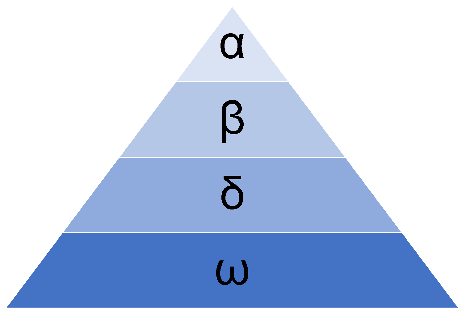
As shown in Figure 2, α is the top of the pyramid and is the head wolf of the grey wolf population. It is not necessarily the most powerful member of the team, but must be the most managerial individual. As the decision maker of the grey wolf population, it is mainly responsible for deciding hunting behaviour, food distribution, and living and resting environments. α ’s appointment is decided by the pack. β is the 2nd level of the pyramid, and belongs to α ’s think-tank team. β assists α in its decision making and deals with the behaviour of the population to some extent. At the same time, β is the queued replacement for the alpha wolf α . When a vacancy occurs in α , β will become the new α . δ is the third level of the pyramid. δ obeys the commands of α and β , can give commands to lower level individuals, and is primarily responsible for scouting, hunting, etc. Older α as well as β will demote to become δ . ω is the lowest level of the pyramid, obeys all other wolves of higher rank, and has the role of balancing relationships within the population.
In the hunting process of the grey wolf, a strict hierarchy represents a very important advantage. Led by α , the pack stalks, chases, and approaches the prey in a dispersed pattern as a team. Then, the wolves surround the prey from all directions, the envelope being determined by α , β and δ in space, while other wolves appear randomly around the prey.
Grey wolves surround their prey while hunting, with α , β , and δ being the three best adapted groups, in that order, guiding ω towards the target. The mathematical model of the grey wolf’s prey search behaviour is represented by the following equation.
D = | C · X p ( t ) X ( t ) |
X ( t + 1 ) = X p ( t ) A · D
where t indicates the current iteration, A and C are coefficient vectors, X p is the position vector of the prey, and X indicates the position vector of a grey wolf.
The vectors A and C are calculated as follows:
A = 2 a · r 1 a
C = 2 · r 2
where components of a are linearly decreased from 2 to 0 over the course of iterations and r 1 and r 2 are random vectors in [ 0 , 1 ] .
In GWO, the optimal solution is defined as α , and the second and third optimal solutions are β and δ . When the grey wolf determines the range of prey locations, α , β , and δ are closest to the prey, and the other wolves in the population use the positions of these three to determine where the prey is and thus move towards the prey.
Equation (22) defines the length and direction of the forward progress of the ω wolf towards α , β , and δ .
D α = | C 1 · X α X | ,   D β = | C 2 · X β X | ,   D δ = | C 3 · X δ X |
where X α , X β , and X δ indicate the current position of the wolves α , β , and δ , respectively, X indicates the current position of the grey wolf, and C indicates a random vector.
X 1 = X α A 1 · D α , X 2 = X β A 2 · D β , X 3 = X δ A 3 · D δ
X ( t + 1 ) = X 1 + X 2 + X 3 3
Equations (23) and (24) define the final position of the ω wolves. The wolf with highest fitness in the final grey wolf population is output as the optimal solution.

3.2. Multi-Threaded Strategy

The standard grey wolf algorithm simulates the hunting process of the grey wolf population as a single-threaded calculation, where one wolf moves to the end of an iterative step before the next wolf can move. At low levels of function complexity, this search is not a problem. However, in the process of parameter inversion, the objective function involves the solution of finite element equations, which is time-consuming. If the single-threaded search method is still used, it will not only result in a high time cost, but also cause the remaining computing resources of the computer to be idle. Taking into account the actual hunting situation of the wolf population and the computing power of computer hardware and software, this paper improves the grey wolf algorithm to multi-threaded parallel computing. The grey wolf population is divided into small groups, with the number of grey wolves in each group being the same as the number of CPU cores in the computer, and the grey wolves in the small groups can act simultaneously. By adopting the multi-threading strategy, the optimisation efficiency can be significantly improved when the computer memory and core resources are abundant.

3.3. Intelligent Models for Parameter Inversion

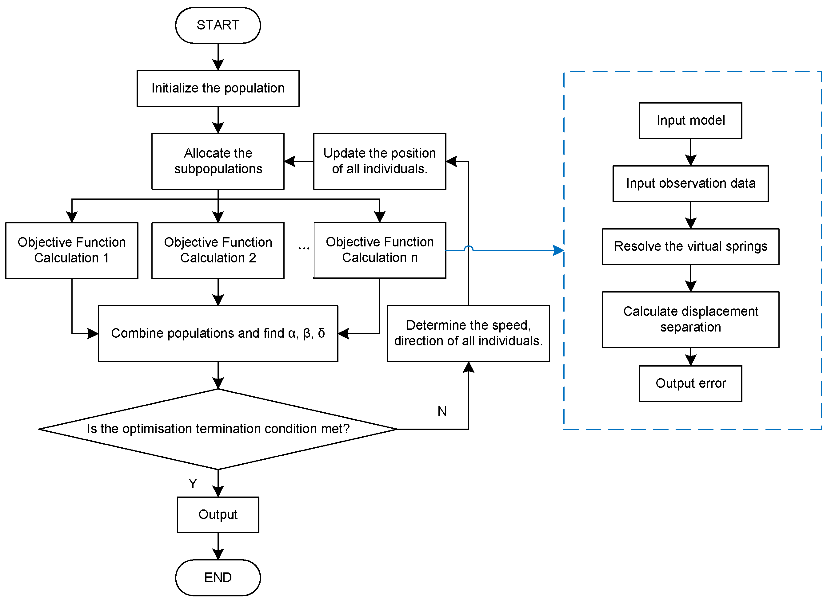
Based on the proposed numerical model and with the aid of GWO, an intelligent inversion model of the dam mechanical parameters can be developed. The model takes the overall error after displacement separation as the objective function value and the mechanical parameters of the dam as the object of optimisation without the need for accurate finite element modelling of the foundation. The flow chart is shown in Figure 3. The implementation steps are as follows:
  • (1) Initialize populations.
  • (2) Assign sub-populations according to computer hardware.
  • (3) Start multi-threaded execution of objective function content.
  • (3.1) Input finite element model and observations.
  • (3.2) Solve the virtual springs.
  • (3.3) Calculate displacement field separation and output RRMSE.
  • (4) Combine populations, and then determine α , β , and δ .
  • (5) Determine if the optimisation termination conditions are met. If so, the calculation is terminated. If not, perform a position update calculation for each individual and repeat steps 2–5.
  • (6) Output the result.
Figure 3. The flowchart of intelligent inversion of parameters.
Water 16 02979 g003

4. Validation

We will devote this section to present a short series of benchmarks, which illustrate the capacity of the proposed separation model. The 2D and 3D cases are verified here separately. The 2D case is used to verify the validity of the numerical model. For the 3D case, we not only verify the validity of the numerical model, but also investigate the effect of the number of virtual springs on the accuracy of the simulation.
A typical section of a gravity dam is used for the 2D case. Based on plane strain assumptions, the state of forces in a gravity dam can be modeled using a 2D section similar to a cantilever beam. A concrete high arch dam is used as a 3D case. Due to the super-static force mechanism of the arch, the 3D model must be used to simulate the deformation of the arch dam.

4.1. 2D Gravity Dam Case

4.1.1. Model

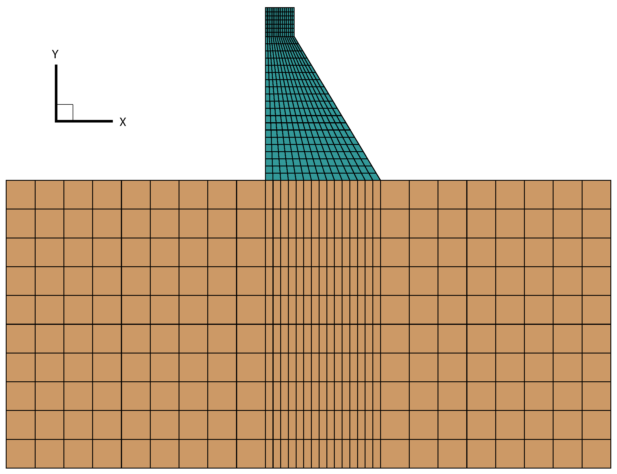
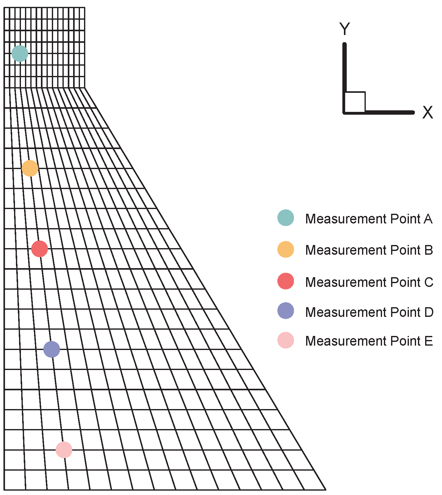
There is a homogeneous concrete gravity dam with a height of 60 m and a width of 30 m, and its cross section is simplified into a two-dimensional model. As shown in Figure 4, the model is discretized into a finite element model with 811 nodes and 740 elements. The foundation extends 1.5 times the height of the dam in the upward, downstream, and depth directions. The truncated boundary adopts displacement constraints. The Young’s modulus of the dam body E d is 23 GPa, and the Poisson’s ratio μ d is 0.167. The Young’s modulus of the foundation rock E f is 30 GPa, and the Poisson’s ratio μ f is 0.200. There are five deformation measurement points in the dam, and Figure 5 shows the positions of them.

4.1.2. Numerical Simulation

Under different water levels, the deformation of the concrete gravity dam is shown in Figure 6. In this paper, h d means the height of the dam and h w means the height of the water.
The virtual springs were set on the contact surface between the dam and the foundation. Except for the foundation constraints, all external effects on the dam were the same.
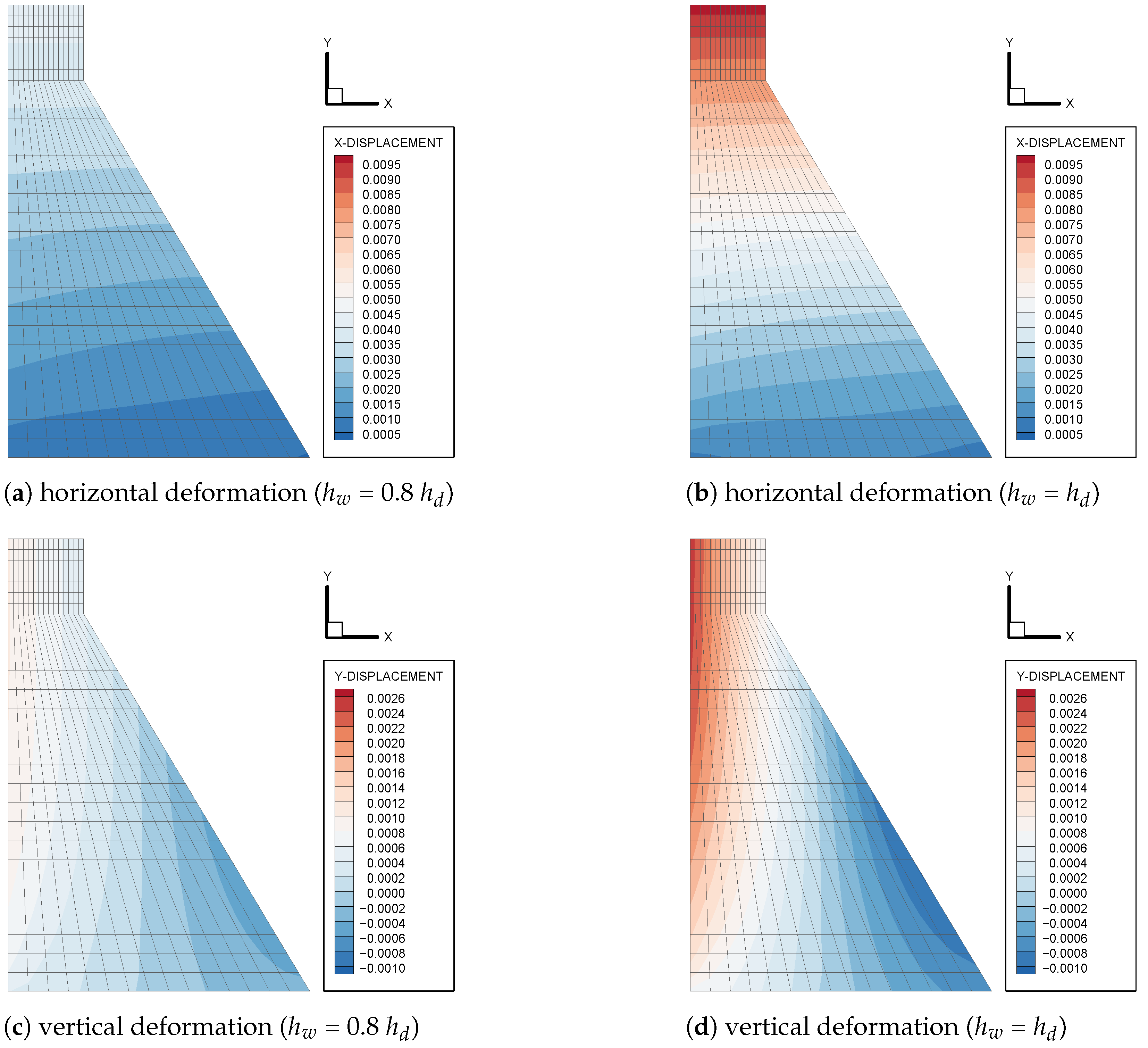
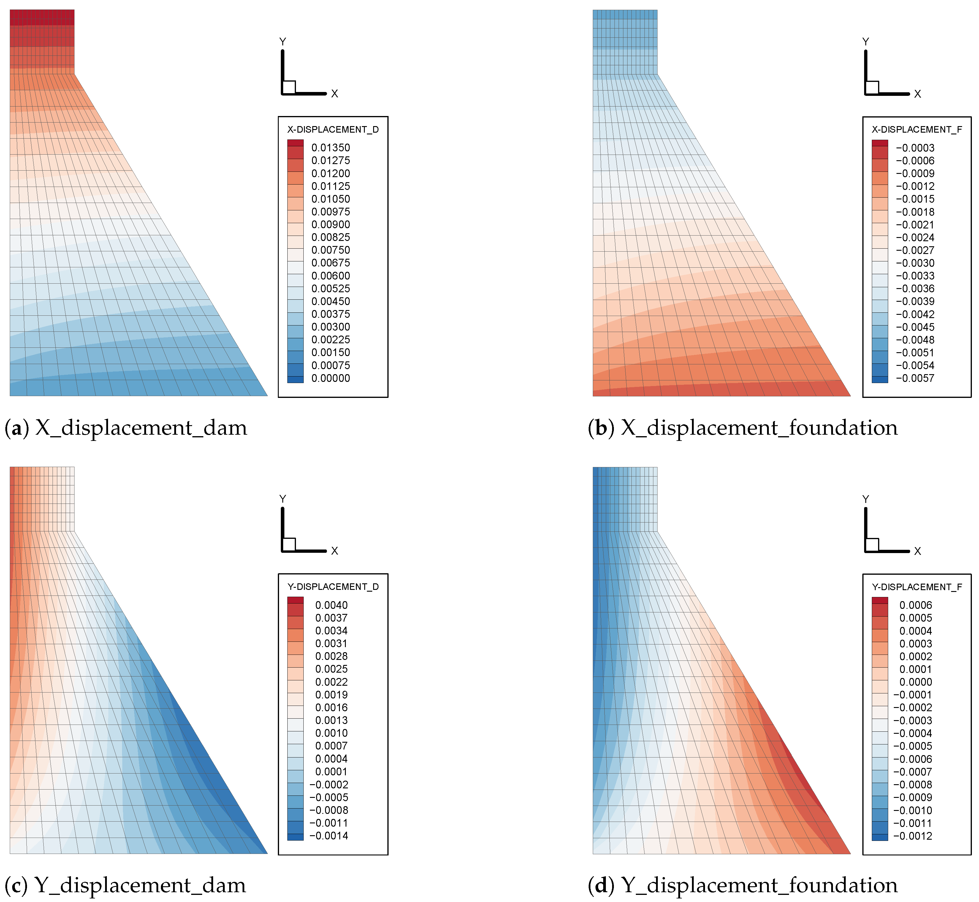
The results of deformation separation under different water levels are shown in Figure 7 and Figure 8. To facilitate comparison between the two different working conditions, we standardized the color range for each type of displacement across both figures. Due to the similarity in errors across the three loading conditions, we present the error analysis for only one condition here to conserve space.
When the water level reached the dam height ( h w = h d ), the displacement values at measurement points obtained through the separation algorithm, along with the observed displacement values and corresponding errors, were recorded. These are shown in Table 1. The Relative Root Mean Square Error (RRMSE) for this condition was 8.4820 × 10 5 , demonstrating the high accuracy of the algorithm in the 2D case.
Analysis of the results reveals distinct deformation patterns: (1) Water load effect: The hydrostatic pressure causes the dam to deform elastically in the downstream direction. (2) Foundation restraint effect: The foundation’s resistance induces an upstream deformation component in the dam.
This interplay suggests that the foundation plays a crucial role in helping the dam resist downstream deformation under water loads. The magnitude and distribution of these deformations vary with water level, as evident from the comparison between Figure 7 and Figure 8.
To further validate the separation model, we compared the calculated displacements ( d c ) with the measured displacements ( d m ) at key points A, B, C, D, and E along the dam profile. The relative errors (RE) for both horizontal (X) and vertical (Y) displacements were consistently low, with most values falling below 0.1%, further confirming the model’s accuracy.
The displacement separation model showed high accuracy across various water levels, effectively distinguishing displacement fields of the dam and foundation for detailed analysis. This capability enhances the understanding of dam–foundation interactions under diverse loading conditions, demonstrating the model’s robustness and adaptability to changing environments, which is critical for real-world dam monitoring. Its successful application to a 2D gravity dam section validates its effectiveness and suggests potential for extension to more complex 3D structures, offering a more nuanced understanding of interactions compared to traditional methods, and thus ensuring the long-term safety and performance of hydraulic structures.

4.2. 3D Arch Dam Case

4.2.1. Model

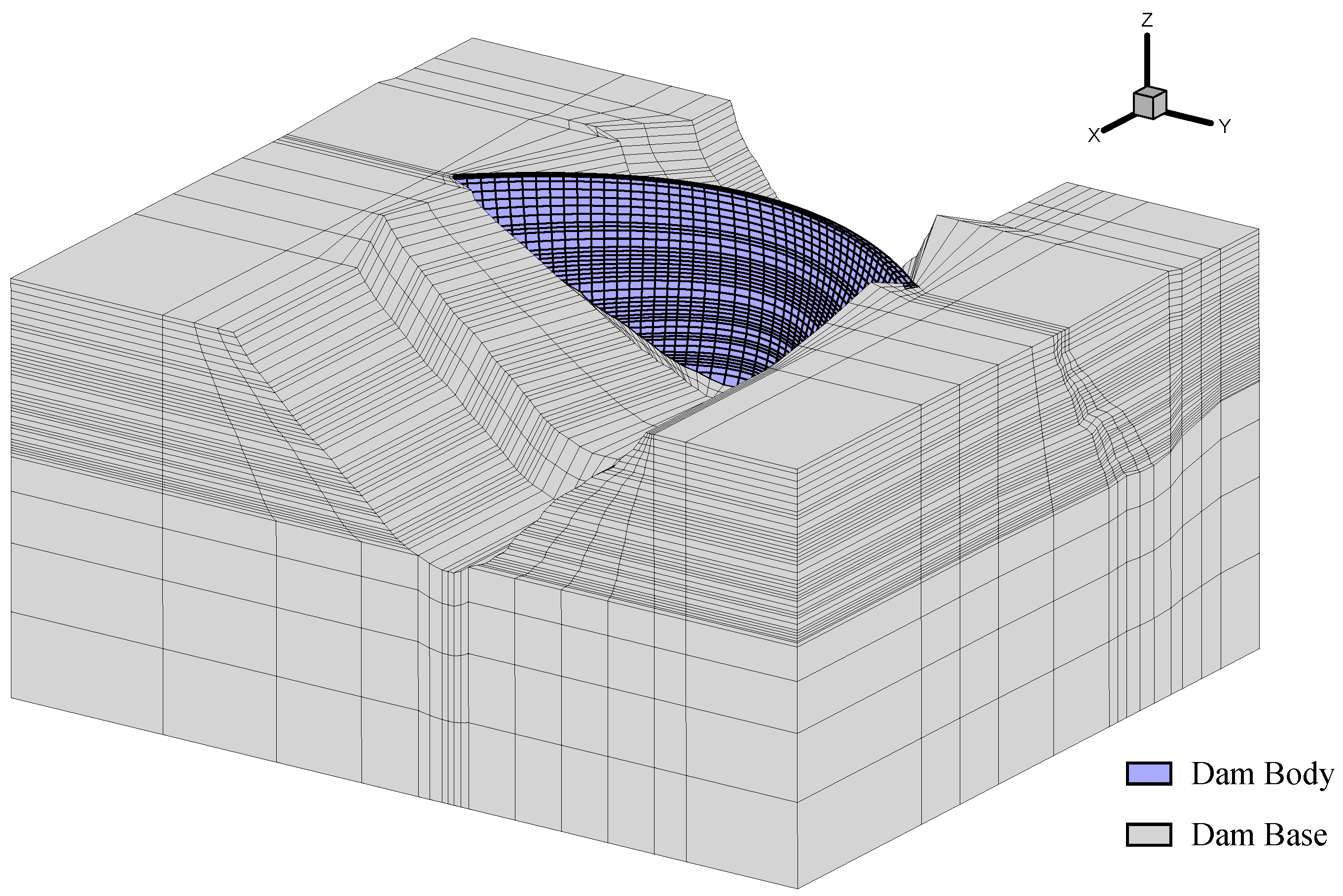
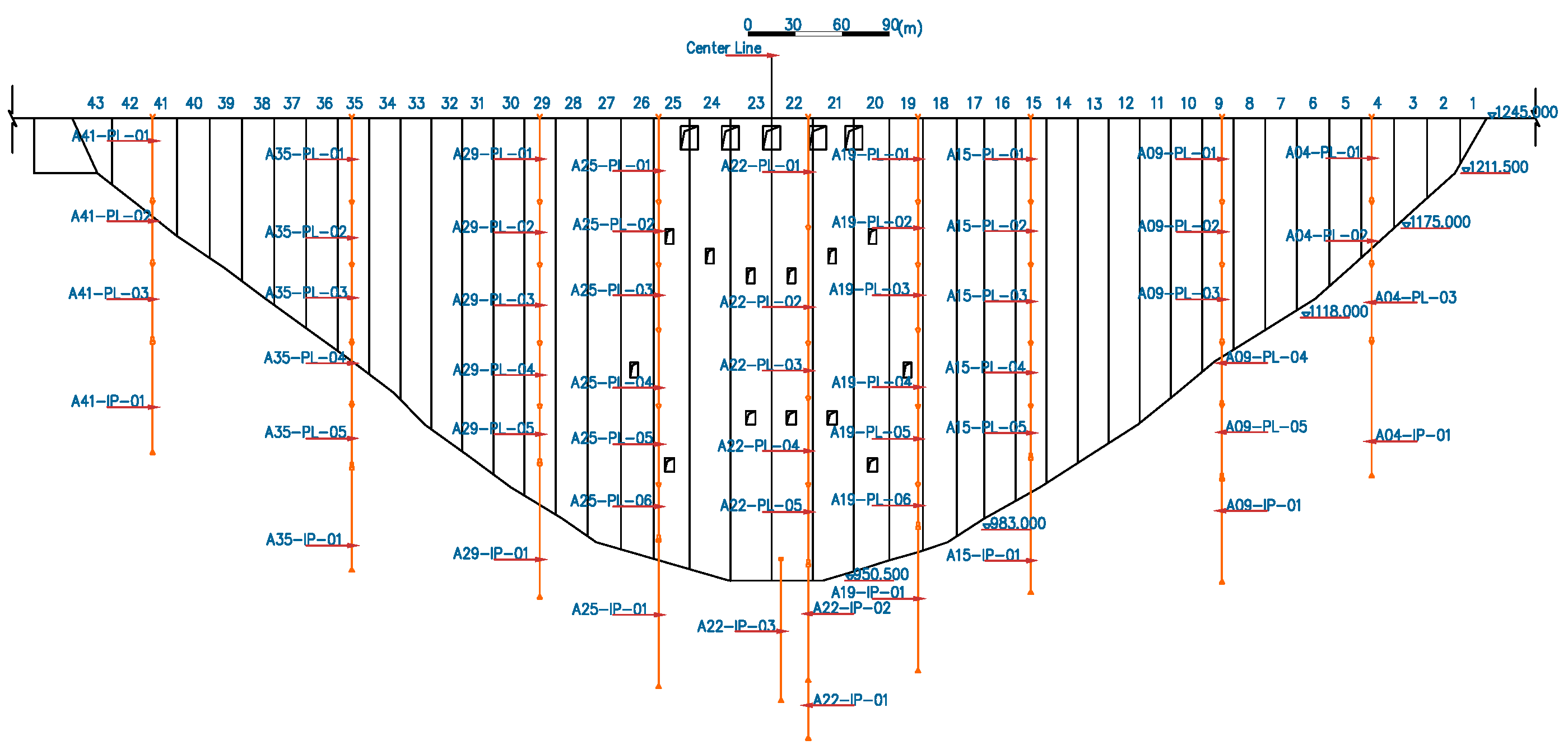
The 3D case is a simplification from an actual engineering project. There is a concrete double-curvature arch dam with a height of 294.5 m, whose FEM model is shown in Figure 9. The FEM model consists of 11,253 nodes and 8382 elements. As an case for verifying the capabilities of the separation model, we keep the physical and mechanical parameters as simple as possible. The dam and foundation are made of homogeneous materials. The Young’s modulus of the dam E d is 23.0 GPa, and the Poisson’s ratio μ d is 0.167. The Young’s modulus of the foundation rock E f is 20.0 GPa, and the Poisson’s ratio μ f is 0.200. The arrangement of the positive and inverted plumb line system is shown in Figure 10.

4.2.2. Numerical Simulation

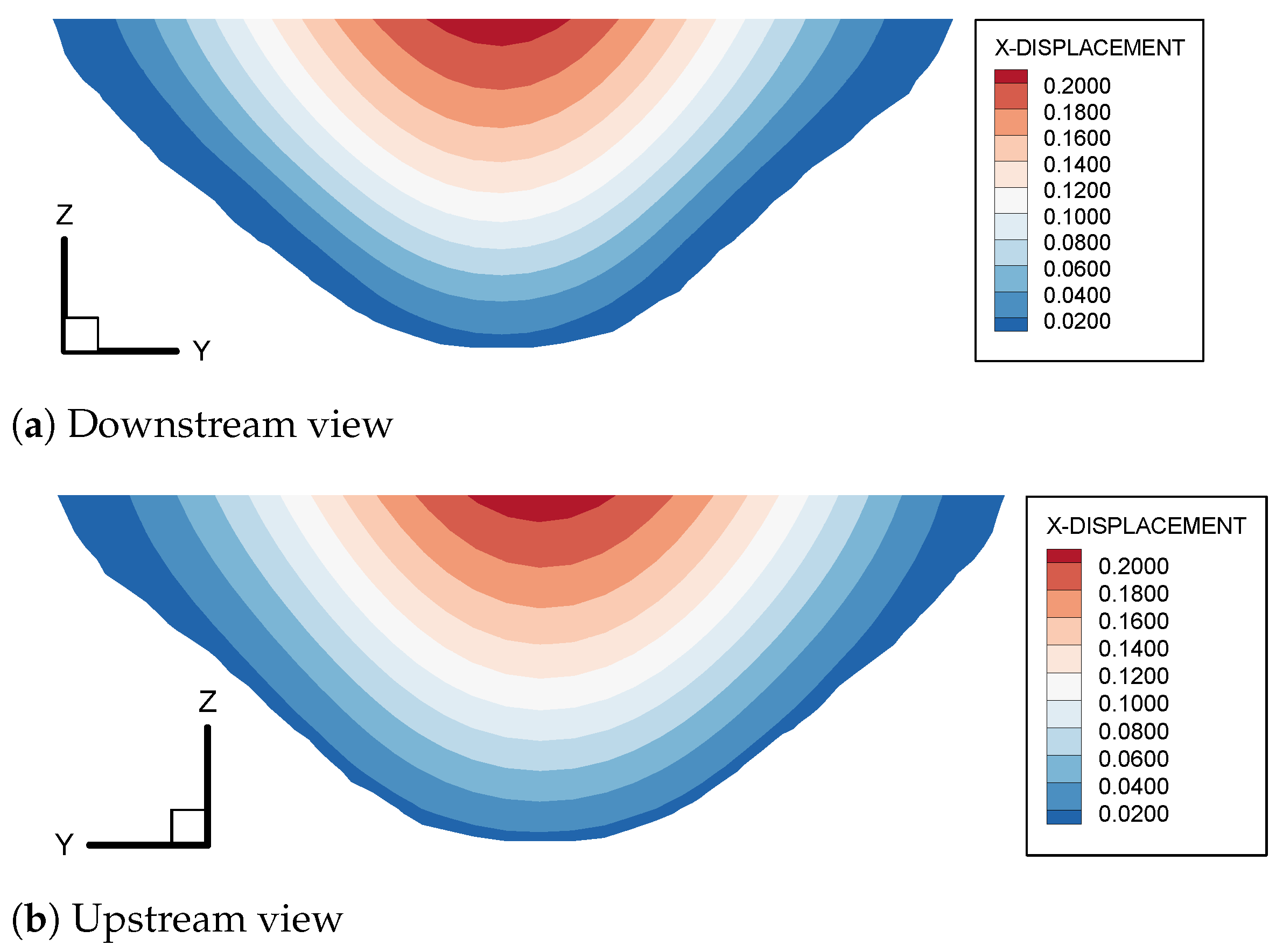
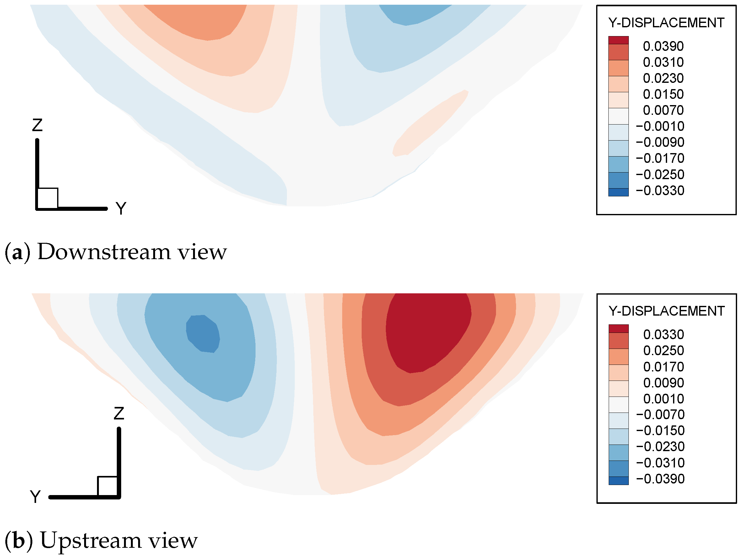
With the load of full water level, the deformation of the arch dam is shown in Figure 11, Figure 12 and Figure 13. It can be seen that the deformation of the arch dam conforms to the normal law.
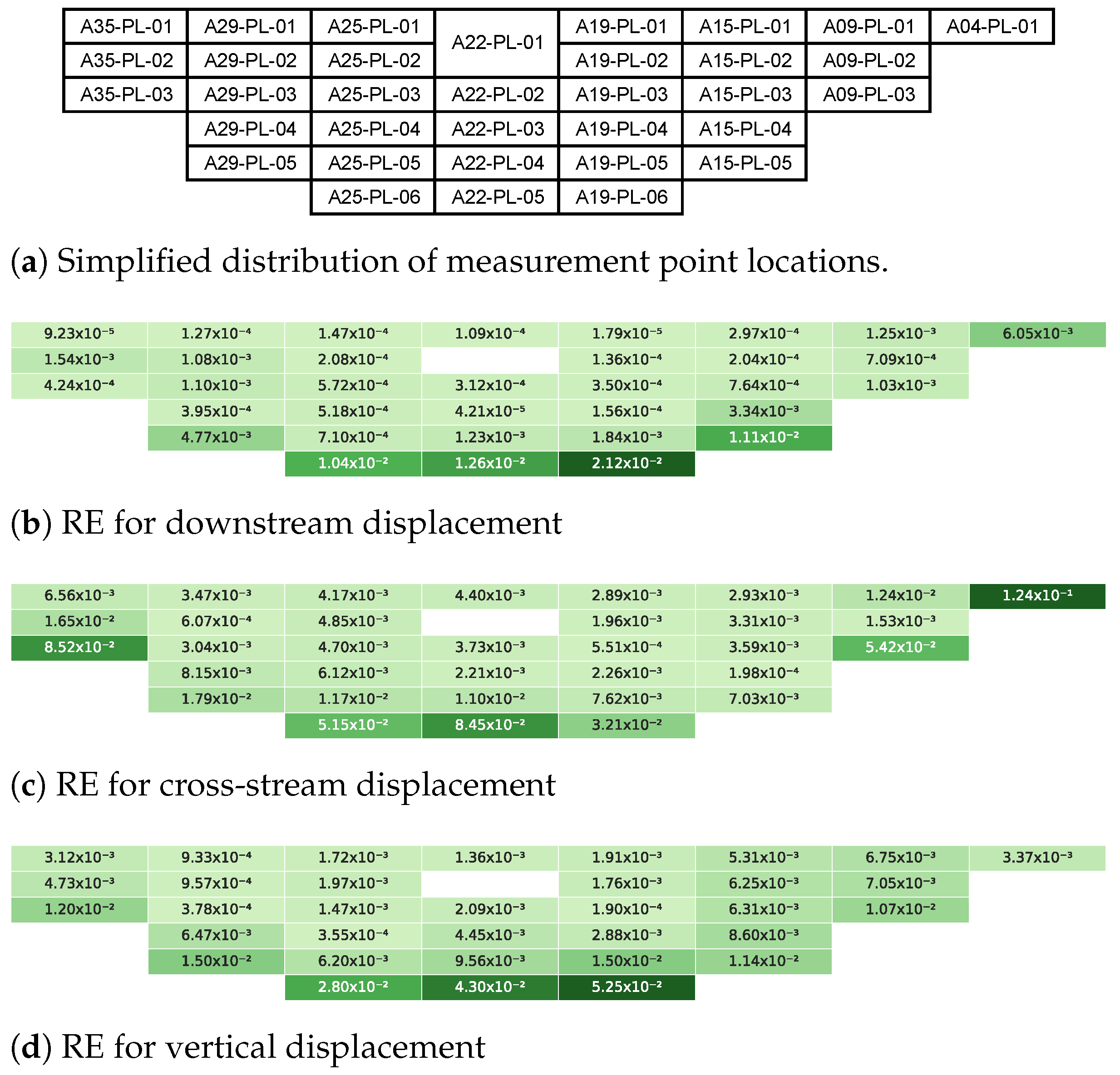
The validity of the separation model on the 3D arch dam was verified first here, and then the effect of the number of springs on the accuracy of the model was explored. Figure 14 shows that the contact surface of the arch dam to the foundation was replaced by five virtual springs. The same water loads were applied to the upstream face of the arch dam as in the forward analysis. A selection of measurement points were selected for analysis based on their actual location in the dam. Figure 15a shows the selected measurement points and their simplified distribution.
Figure 15b–d illustrate the RE for each of the selected measurement points in the downstream, cross-stream, and vertical directions, respectively. It can be seen that the error in the area close to the foundation was greater than the error in the other areas. For the cross-stream displacement, the error near the shoulder of the dam was greater than the error at other areas. The overall pattern shows that the further away from the foundation of the dam the measurement point is, the smaller its error will be. It can be seen that the errors in the results for all measurement points are small and within the acceptable error range for the engineering analysis, indicating that the proposed separation model is effective and reasonable for the displacement separation of the dam.
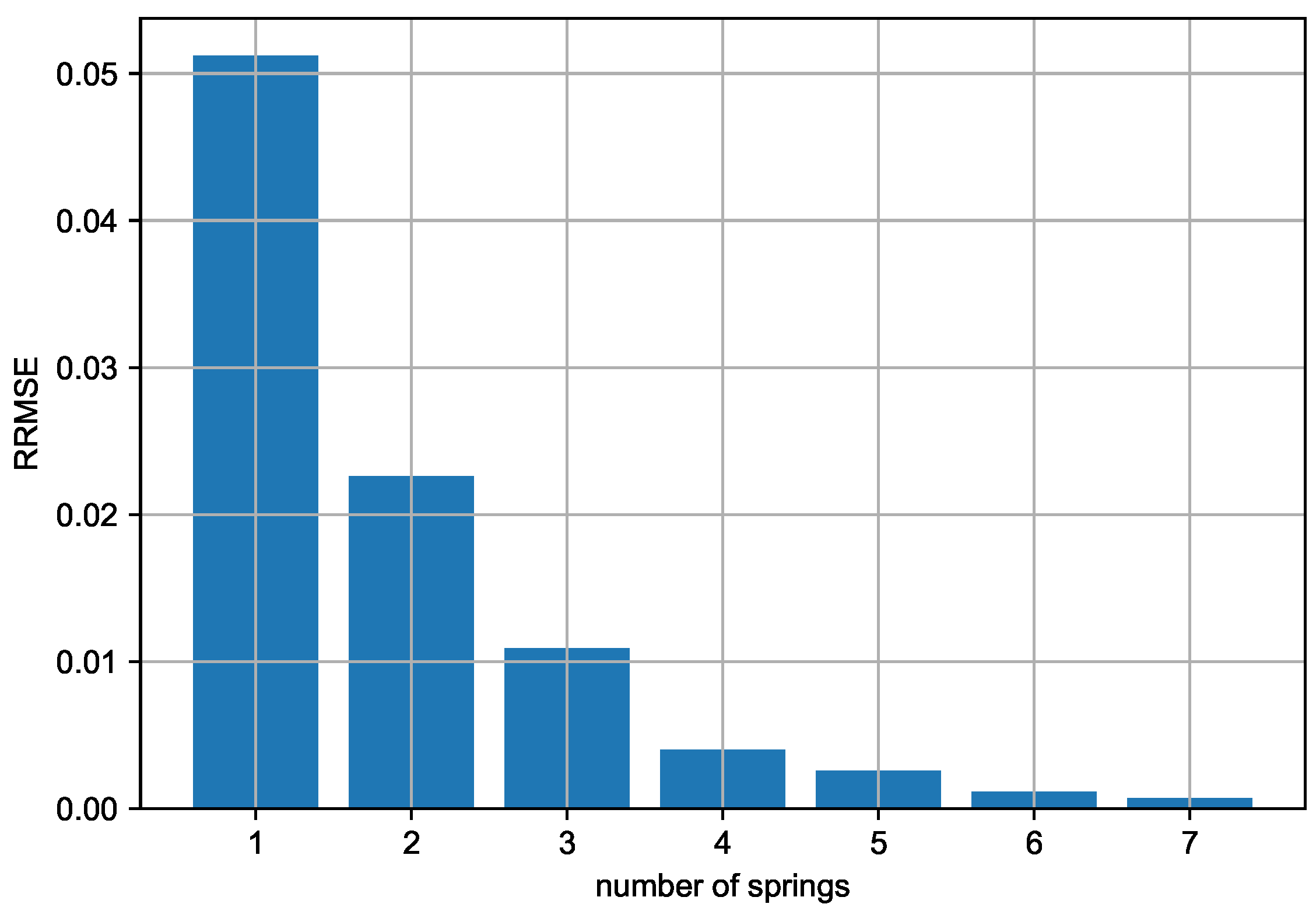
To study the effect of the number of virtual springs on the accuracy of the separation model, different numbers of springs were installed on the foundation surface of the arch dam. Figure 16 shows the RRMSE for different numbers of virtual springs. As the number of virtual springs increased, the RRMSE decreased. However, when the number of springs was greater than four, the reduction of RRMSE became no longer significant. It can be assumed that the number of springs given the dam constraints is close to optimal with the current amount of measurement data. It can be considered that the error was already small when five virtual springs were used, and the continued increase in the number of springs was no longer significant in improving the accuracy of this case.

5. An Application in the Health Diagnosis of a High Arch Dam in China

In southwestern China, there is a ultra-high concrete arch dam which has been in operation for several years since its completion. In fact, in the previous 3D case, we used its model as a validation example. As shown in Figure 9, the height of the dam is 294.50 m. The elevation of the bottom of the dam is 950.50 m, and the elevation of the top is 1245.00 m. The reservoir’s calibration level is 1242.51 m, with a total storage capacity of 15 billion m 3 . The normal storage level is 1240.00 m, the dead level is 1166.00 m, and the regulating reservoir capacity is 9.90 billion m3. The main project at this dam is power generation, and also has the benefit of comprehensive use in areas such as flood control. This extra-high concrete arch dam has an important role to play in the deployment of water resources and energy supply in southwestern China.

5.1. Model

The concrete material of the dam has three divisions, as shown in Figure 17. Division A is dominated by dam sections 1–4, 40–43, the thrust abutment, the remaining dam sections at 20–40 m height from the foundation, and sections 20–25 above 1130 m elevation. Division B is the portion containing dam sections 5–39 outside of division A and C. Division C is between dam sections 8 and 17 and dam sections 28 and 36 between 1107 and 1218 m elevation. The test values of the physical and mechanical parameters of the concrete for each division are shown in Table 2.
Various types of monitoring were set up for this project, including deformation, temperature, stress, cracks, etc. Plumb lines were installed in the galleries of each level of dam sections 4, 9, 15, 22, 29, 35 and 41 to monitor the horizontal deformation and deflection of the dam. Field information indicated poor quality plumb-line monitoring data for dam sections 4 and 41. The instruments were considered to be possibly faulty or subject to persistent external interference. In the analysis, data from these two dam sections were not incorporated in the calculations. The layout of the plumb line system for the arch dam is shown in Figure 10. The vertical deformation measurement points were placed at the top and inside each dam section at elevations of 1245 m, 1190 m, and 1150 m respectively. Thermometers were installed on the downstream face and inside of dam sections 9, 15, 22, 29, and 35.
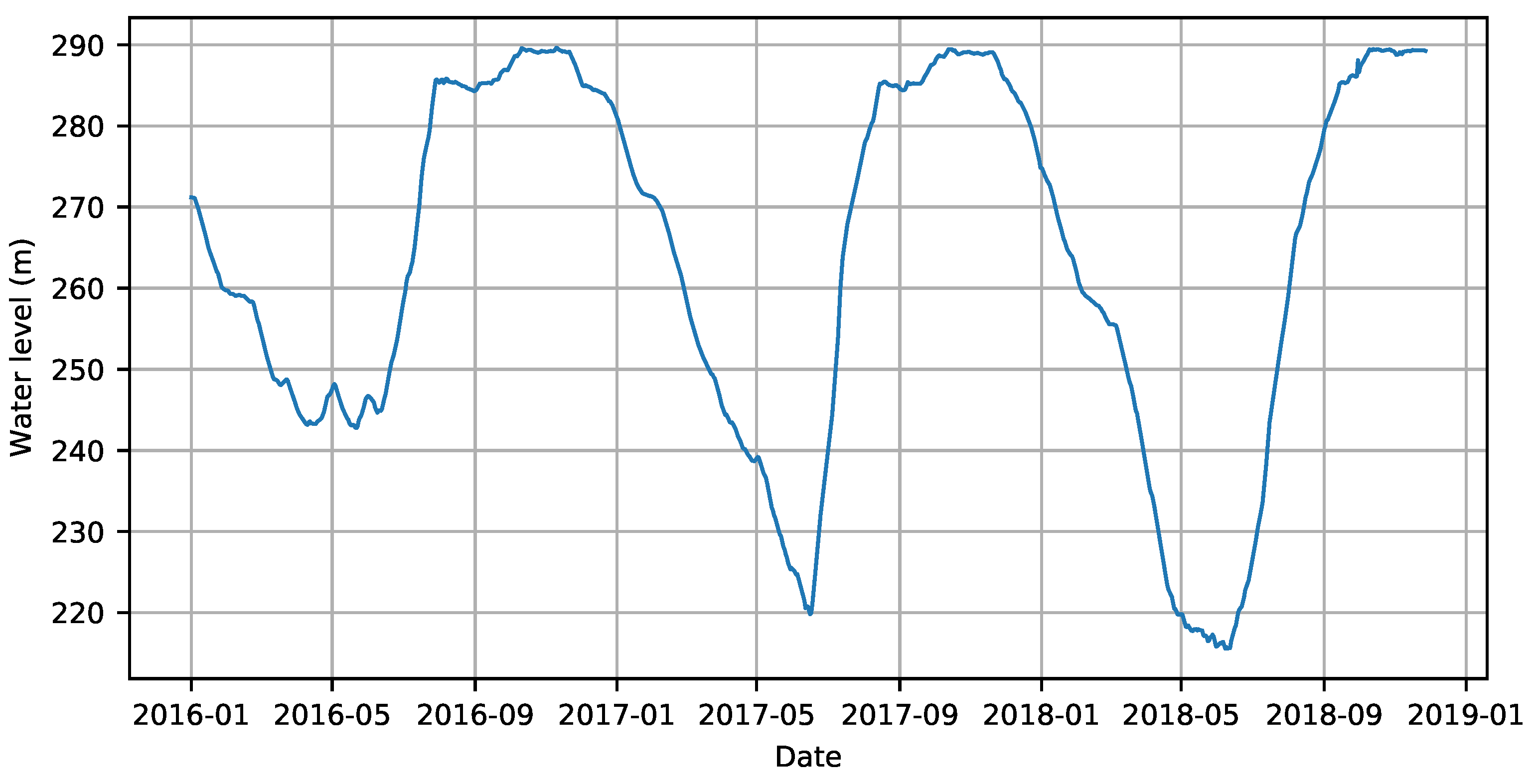
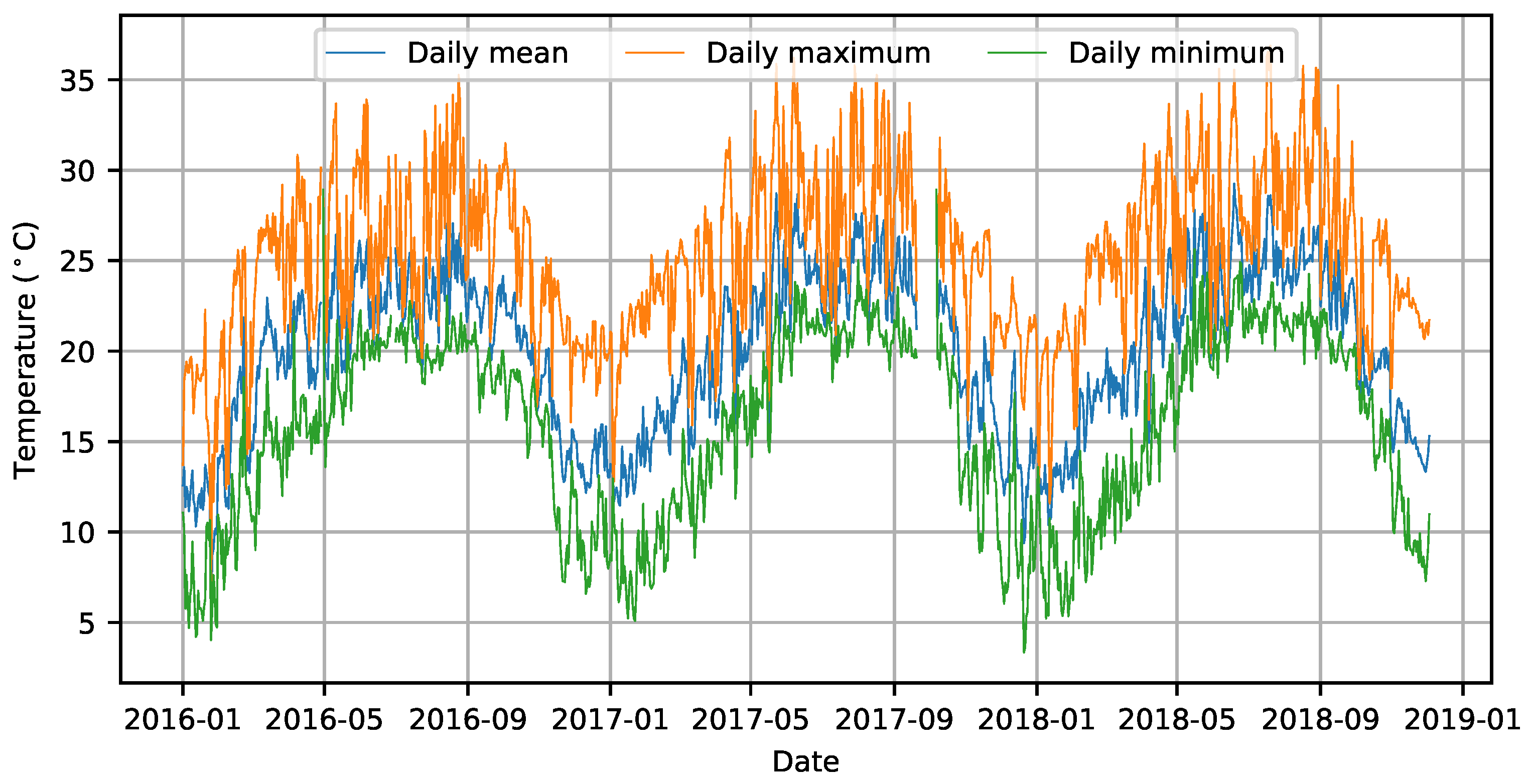
The three years from 2016 to 2018 were chosen as the period of analysis. The water level and air temperature during the period are shown in Figure 18 and Figure 19. The measured values of downstream displacement of some plumb lines are shown in Figure 20.

5.2. Parameter Inverted and Discussion

As the construction process of this arch dam lasted for a considerable period of time, the start-up times of the various measurement instruments varied. For the purpose of analysis, the relative changes in the displacement field during dynamic changes in water level during operation are used as the measured information.
As an important load on arch dam, temperature should be considered in the simulation of a case. The thermodynamic boundary conditions are as follows: (1) the measured water temperature is used for the temperature of the dam surface below the water level, because of the large surface exothermic coefficient at the part of the concrete in contact with water; (2) the measured value of the thermometer near the surface of the dam surface is used for the part of the concrete in contact with air; (3) the measured water temperature is used for the part of the river valley bank below the water surface, and the average air temperature is used for the part above the water surface; and (4) the side of the foundation is treated as an adiabatic boundary. The nodal forces of the dam obtained from the temperature field simulations were added to the dam model as external loads.
As there may be temporal changes in the concrete of the dam, the observations from 2016, 2017, and 2018 were analysed separately. The analysis of the calculated results for the different years is likewise an important element of the health diagnosis. The Young’s modulus of the three zones of the concrete arch dam were inverted as unknown parameters without considering the foundation. The goal of the optimisation process was to ensure that the dam deformation obtained based on the separation model was closest to the measured displacement field.
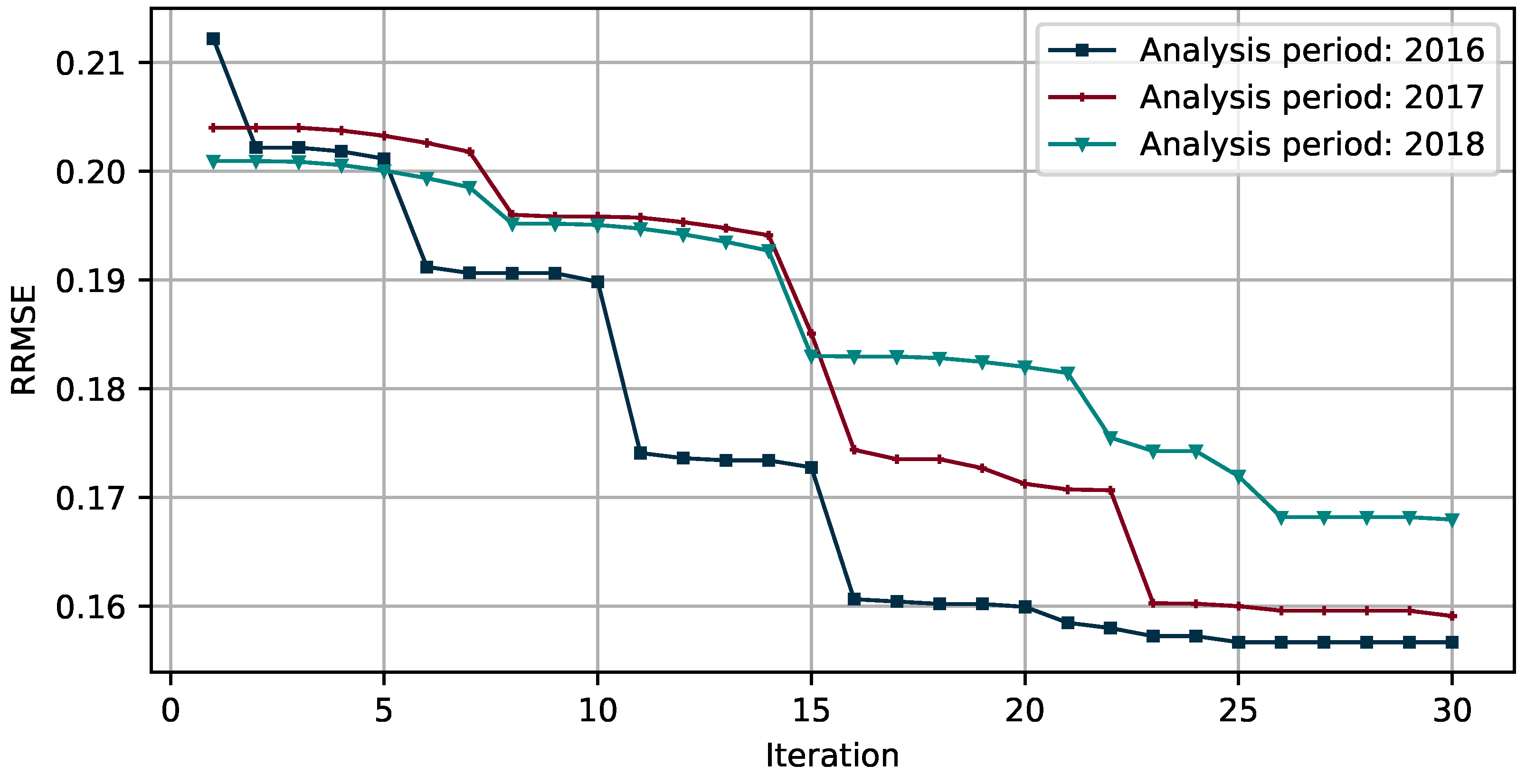
Based on the study of the number of virtual springs, the constraint of the foundation on the dam body was replaced by six virtual springs considering the distribution of measurement points and modeling efficiency. The measured data were sampled at a frequency of 10 days. In the optimisation model, the number of iteration steps was set to 30 and the population size to 24. RRMSE was used as the fitness of the optimisation method. The optimisation processes for the three time periods are shown in Figure 21, and the result of the Young’s modulus inversion is shown in Table 3.
As can be seen from the above results, the Young’s modulus of each part of the concrete did not change much across the three years. As concrete is a non-homogeneous material and the environment in which it is placed varies from part to part, there may be different trends in long-term operation. Whereas test sampling can only obtain data from local samples, Young’s modulus obtained by inverse analysis of observed data from multiple measurement points is more representative of the overall performance of the concrete material in the dam. The Young’s modulus values for concrete obtained in this paper are at a reasonable level when compared to other similar engineering projects. Based on the analysis results, we consider this high arch dam to be currently in a healthy structural condition.

6. Conclusions

In this paper we analysed the main difficulties in the health diagnosis and parameter inversion of concrete dams, focusing mainly the uncertainty in the foundations, which can have a large impact on the numerical analysis. We proposed a constrained displacement separation model, which uses a number of virtual springs to simulate the constraints of the foundation on the deformation of the dam and achieves displacement separation based on observed data. In combination with the swarm intelligence optimisation method, the displacement separation model can be used to identify dam deformation parameters for concrete gravity dams and arch dams in operation. The following conclusions can be made:
(1)
The displacement separation model proposed in this paper can be applied to the solution of multiple degrees of freedom, including two-dimensional gravity dam sections, three-dimensional arch dams, or gravity dams, as verified by calculation cases. In the case of sufficient measurement data, as the number of virtual springs increases, the model accuracy will increase, but the trend of improvement will slow down.
(2)
In combination with the interpolation of displacement fields, it is no longer necessary to make element nodes coincide with measurement points when modelling the dam, improving the simplicity of modelling the separation model.
(3)
Applying multi-threaded strategies to swarm intelligence optimisation methods can improve computational efficiency. When the method is executed on a computer with a multi-core processor, results can be obtained quickly. Using the error in displacement separation as an objective function, combined with an optimisation method, it is possible to achieve a rapid inverse analysis of the deformation parameters of a concrete dam without the need to determine physical mechanical parameters of the foundation.
(4)
The model proposed in this paper was successfully applied to the structural health diagnosis of a very high concrete arch dam in southern China. Rapid identification of concrete deformation parameters in three zones of the dam body was achieved with reasonable results. As an accurate and efficient structural diagnosis model for concrete dams that does not require assumptions about foundation parameters, it can provide a reference for structural health diagnosis of concrete dams during operation.
Based on the research presented in this paper, several directions for future work can be identified:
(1)
Advanced sensing and data integration: Incorporate data from emerging technologies like distributed fiber optic sensors and wireless sensor networks to provide more comprehensive information about dam behavior. This would enable more accurate parameter inversion and health diagnosis, potentially revealing subtle changes in dam performance that current methods might miss.
(2)
Machine learning enhancement: Explore the application of deep learning algorithms, such as convolutional neural networks or recurrent neural networks, to improve the accuracy and efficiency of parameter inversion. These techniques could be particularly effective in handling large datasets and capturing complex, non-linear relationships in dam behavior, potentially leading to more robust and adaptive health monitoring systems.
(3)
Multi-physics modeling and long-term monitoring: Extend the approach to include coupled thermal-structural analysis or even hydro-mechanical-thermal coupling for a more comprehensive understanding of dam behavior. Develop a framework for continuous monitoring and analysis using the proposed method, enabling predictive maintenance strategies and early warning systems based on detected changes in inverted parameters over time.
These future directions aim to further enhance the accuracy, efficiency, and applicability of the proposed method for concrete dam health diagnosis and parameter inversion. By addressing these areas, we can continue to improve the safety and longevity of critical infrastructure like dams.

Author Contributions

Methodology and Software, T.L.; Resources, J.X. and Y.P.; Data curation, J.G. and J.W.; Writing—original draft, L.G.; Writing—review & editing, H.Q.; Supervision, J.X. All authors have read and agreed to the published version of the manuscript.

Funding

This work is financially supported by the National Key R&D Program (SN: 2021YFC3090105), the National Natural Science Foundation of China (SN: 52009035).

Data Availability Statement

The data presented in this study are available on request from the corresponding author. The data are not publicly available due to privacy.

Conflicts of Interest

The authors declare no conflicts of interest.

References

  1. Jia, J. A Technical Review of Hydro-Project Development in China. Engineering 2016, 2, 302–312. [Google Scholar] [CrossRef]
  2. Ren, Q.; Li, M.; Song, L.; Liu, H. An optimized combination prediction model for concrete dam deformation considering quantitative evaluation and hysteresis correction. Adv. Eng. Inform. 2020, 46, 101154. [Google Scholar] [CrossRef]
  3. Shao, C.; Gu, C.; Yang, M.; Xu, Y.; Su, H. A novel model of dam displacement based on panel data. Struct. Control Health Monit. 2018, 25, e2037. [Google Scholar] [CrossRef]
  4. Feng, X.T.; Zhang, Z.; Sheng, Q. Estimating mechanical rock mass parameters relating to the Three Gorges Project permanent shiplock using an intelligent displacement back analysis method. Int. J. Rock Mech. Min. Sci. 2000, 37, 1039–1054. [Google Scholar] [CrossRef]
  5. Stojanovic, B.; Milivojevic, M.; Milivojevic, N.; Antonijevic, D. A self-tuning system for dam behavior modeling based on evolving artificial neural networks. Adv. Eng. Softw. 2016, 97, 85–95. [Google Scholar] [CrossRef]
  6. Kang, F.; Liu, X.; Li, J.; Li, H. Multi-parameter inverse analysis of concrete dams using kernel extreme learning machines-based response surface model. Eng. Struct. 2022, 256, 113999. [Google Scholar] [CrossRef]
  7. Azmi, M.; Paultre, P. Three-dimensional analysis of concrete dams including contraction joint non-linearity. Eng. Struct. 2002, 24, 757–771. [Google Scholar] [CrossRef]
  8. Kao, C.Y.; Loh, C.H. Monitoring of long-term static deformation data of Fei-Tsui arch dam using artificial neural network-based approaches. Struct. Control Health Monit. 2013, 20, 282–303. [Google Scholar] [CrossRef]
  9. Habib, P. The Malpasset Dam failure. Eng. Geol. 1987, 24, 331–338. [Google Scholar] [CrossRef]
  10. Roth, S.N.; Léger, P.; Soulaïmani, A. Strongly coupled XFEM formulation for non-planar three-dimensional simulation of hydraulic fracturing with emphasis on concrete dams. Comput. Methods Appl. Mech. Eng. 2020, 363, 112899. [Google Scholar] [CrossRef]
  11. Ardito, R.; Maier, G.; Massalongo, G. Diagnostic analysis of concrete dams based on seasonal hydrostatic loading. Eng. Struct. 2008, 30, 3176–3185. [Google Scholar] [CrossRef]
  12. Szostak-Chrzanowski, A.; Chrzanowski, A.; Massiéra, M. Use of deformation monitoring results in solving geomechanical problems - Case studies. Eng. Geol. 2005, 79, 3–12. [Google Scholar] [CrossRef]
  13. Sharifzadeh, M.; Tarifard, A.; Moridi, M.A. Time-dependent behavior of tunnel lining in weak rock mass based on displacement back analysis method. Tunn. Undergr. Space Technol. 2013, 38, 348–356. [Google Scholar] [CrossRef]
  14. De Sortis, A.; Paoliani, P. Statistical analysis and structural identification in concrete dam monitoring. Eng. Struct. 2007, 29, 110–120. [Google Scholar] [CrossRef]
  15. Agullo, L.; Mirambell, E.; Aguado, A. A model for the analysis of concrete dams due to environmental thermal effects. Int. J. Numer. Methods Heat Fluid Flow 1996, 6, 25–36. [Google Scholar] [CrossRef]
  16. Stojanovic, B.; Milivojevic, M.; Ivanovic, M.; Milivojevic, N.; Divac, D. Adaptive system for dam behavior modeling based on linear regression and genetic algorithms. Adv. Eng. Softw. 2013, 65, 182–190. [Google Scholar] [CrossRef]
  17. Wei, B.; Chen, L.; Li, H.; Yuan, D.; Wang, G. Optimized prediction model for concrete dam displacement based on signal residual amendment. Appl. Math. Model. 2020, 78, 20–36. [Google Scholar] [CrossRef]
  18. Mata, J.; Tavares De Castro, A.; Sá Da Costa, J. Constructing statistical models for arch dam deformation. Struct. Control Health Monit. 2014, 21, 423–437. [Google Scholar] [CrossRef]
  19. Salazar, F.; Toledo, M.T.; Oñate, E.; Suárez, B. Interpretation of dam deformation and leakage with boosted regression trees. Eng. Struct. 2016, 119, 230–251. [Google Scholar] [CrossRef]
  20. Kang, F.; Liu, J.; Li, J.; Li, S. Concrete dam deformation prediction model for health monitoring based on extreme learning machine. Struct. Control Health Monit. 2017, 24, 1997. [Google Scholar] [CrossRef]
  21. Dai, B.; Gu, C.; Zhao, E.; Qin, X. Statistical model optimized random forest regression model for concrete dam deformation monitoring. Struct. Control Health Monit. 2018, 25, e2170. [Google Scholar] [CrossRef]
  22. Kang, F.; Li, J.; Zhao, S.; Wang, Y. Structural health monitoring of concrete dams using long-term air temperature for thermal effect simulation. Eng. Struct. 2019, 180, 642–653. [Google Scholar] [CrossRef]
  23. Fedele, R.; Maier, G.; Miller, B. Health assessment of concrete dams by overall inverse analyses and neural networks. Int. J. Fract. 2006, 137, 151–172. [Google Scholar] [CrossRef]
  24. Bonaldi, P.; Fanelli, M.; Giuseppetti, G. Displacement Forecasting for Concrete Dams. Int. Water Power Dam Constr. 1977, 29, 42–50. [Google Scholar] [CrossRef]
  25. Zienkiewicz, O.; Taylor, R.; Zhu, J. The Finite Element Method for Solid and Structural Mechanics; Elsevier: Amsterdam, The Netherlands, 2005. [Google Scholar]
  26. Li, H.; Wang, G.; Wei, B.; Zhong, Y.; Zhan, L. Dynamic inversion method for the material parameters of a high arch dam and its foundation. Appl. Math. Model. 2019, 71, 60–76. [Google Scholar] [CrossRef]
  27. Bocciarelli, M.; Ranzi, G. An inverse analysis approach for the identification of the hygro-thermo-chemical model parameters of concrete. Int. J. Mech. Sci. 2018, 138–139, 368–382. [Google Scholar] [CrossRef]
  28. Zhou, W.; Li, S.L.; Ma, G.; Chang, X.L.; Ma, X.; Zhang, C. Parameters inversion of high central core rockfill dams based on a novel genetic algorithm. Sci. China Technol. Sci. 2016, 59, 783–794. [Google Scholar] [CrossRef]
  29. Yazdani, M.; Sharifzadeh, M.; Kamrani, K.; Ghorbani, M. Displacement-based numerical back analysis for estimation of rock mass parameters in Siah Bisheh powerhouse cavern using continuum and discontinuum approach. Tunn. Undergr. Space Technol. 2012, 28, 41–48. [Google Scholar] [CrossRef]
  30. Oreste, P. Back-analysis techniques for the improvement of the understanding of rock in underground constructions. Tunn. Undergr. Space Technol. 2005, 20, 7–21. [Google Scholar] [CrossRef]
  31. Guo, Q.; Pei, L.; Zhou, Z.; Chen, J.; Yao, F. Response surface and genetic method of deformation back analysis for high core rockfill dams. Comput. Geotech. 2016, 74, 132–140. [Google Scholar] [CrossRef]
  32. Yang, L.; Su, H.; Wen, Z. Improved PLS and PSO methods-based back analysis for elastic modulus of dam. Adv. Eng. Softw. 2019, 131, 205–216. [Google Scholar] [CrossRef]
  33. Lin, C.; Li, T.; Chen, S.; Lin, C.; Liu, X.; Gao, L.; Sheng, T. Structural identification in long-term deformation characteristic of dam foundation using meta-heuristic optimization techniques. Adv. Eng. Softw. 2020, 148, 102870. [Google Scholar] [CrossRef]
  34. Yang, L.; Wen, Z.; Yan, X.; Hua, Q.; Su, H. Structural inverse analysis of concrete dams: Considering residual hydration heat effect on dam displacements. Eng. Comput. 2023, 39, 2829–2849. [Google Scholar] [CrossRef]
  35. Wang, S.; Xu, C.; Liu, Y.; Xu, B. Zonal intelligent inversion of viscoelastic parameters of high arch dams using an HEST statistical model. J. Civ. Struct. Health Monit. 2022, 12, 207–223. [Google Scholar] [CrossRef]
  36. Zhang, W.; Xu, L.; Shen, Z.; Ma, B. A new approach for mechanical parameter inversion analysis of roller compacted concrete dams using modified PSO and RBFNN. Clust. Comput. 2022, 25, 4633–4652. [Google Scholar] [CrossRef]
  37. Zienkiewicz, O.C. Achievements and some unsolved problems of the finite element method. Int. J. Numer. Methods Eng. 2000, 47, 9–28. [Google Scholar] [CrossRef]
  38. Uriarte, C.; Pardo, D.; Omella, Á.J. A Finite Element based Deep Learning solver for parametric PDEs. Comput. Methods Appl. Mech. Eng. 2022, 391, 114562. [Google Scholar] [CrossRef]
  39. Lin, C.; Li, T.; Liu, X.; Zhao, L.; Chen, S.; Qi, H. A deformation separation method for gravity dam body and foundation based on the observed displacements. Struct. Control Health Monit. 2019, 26, 1–18. [Google Scholar] [CrossRef]
  40. Li, T.; He, J.; Zhao, L.; Li, X.; Niu, Z. Strength reduction method for stability analysis of local discontinuous rock mass with iterative method of partitioned finite element and interface boundary element. Math. Probl. Eng. 2015, 2015, 872834. [Google Scholar] [CrossRef]
  41. Fan, S.; Li, T.; Liu, X.; Zhao, L.; Niu, Z.; Qi, H. A hybrid algorithm of partitioned finite element and interface element for dynamic contact problems with discontinuous deformation. Comput. Geotech. 2018, 101, 130–140. [Google Scholar] [CrossRef]
  42. Gao, L.; Li, T.; Liu, X.; Qi, H.; Fan, S.; Lin, C.; Zhou, M. A novel dynamic stability analysis method for jointed rock slopes based on block-interface interaction. Comput. Geotech. 2021, 134, 104113. [Google Scholar] [CrossRef]
  43. Qi, H.; Li, T.; Liu, X.; Zhao, L.; He, J.; Li, X. A fast local nonlinear solution technique based on the partitioned finite element and interface element method. Int. J. Numer. Methods Eng. 2022, 123, 2214–2236. [Google Scholar] [CrossRef]
  44. Salazar, F.; Vicente, D.J.; Irazábal, J.; De-Pouplana, I.; San Mauro, J. A Review on Thermo-mechanical Modelling of Arch Dams During Construction and Operation: Effect of the Reference Temperature on the Stress Field. Arch. Comput. Methods Eng. 2020, 27, 1681–1707. [Google Scholar] [CrossRef]
  45. Soltani, N.; Alembagheri, M.; Khaneghahi, M.H. Risk-based probabilistic thermal-stress analysis of concrete arch dams. Front. Struct. Civ. Eng. 2019, 13, 1007–1019. [Google Scholar] [CrossRef]
  46. Mirjalili, S.; Mirjalili, S.M.; Lewis, A. Grey Wolf Optimizer. Adv. Eng. Softw. 2014, 69, 46–61. [Google Scholar] [CrossRef]
  47. Emary, E.; Zawbaa, H.M.; Hassanien, A.E. Binary grey wolf optimization approaches for feature selection. Neurocomputing 2016, 172, 371–381. [Google Scholar] [CrossRef]
  48. Li, E.; Yang, F.; Ren, M.; Zhang, X.; Zhou, J.; Khandelwal, M. Prediction of blasting mean fragment size using support vector regression combined with five optimization algorithms. J. Rock Mech. Geotech. Eng. 2021, 13, 1380–1397. [Google Scholar] [CrossRef]
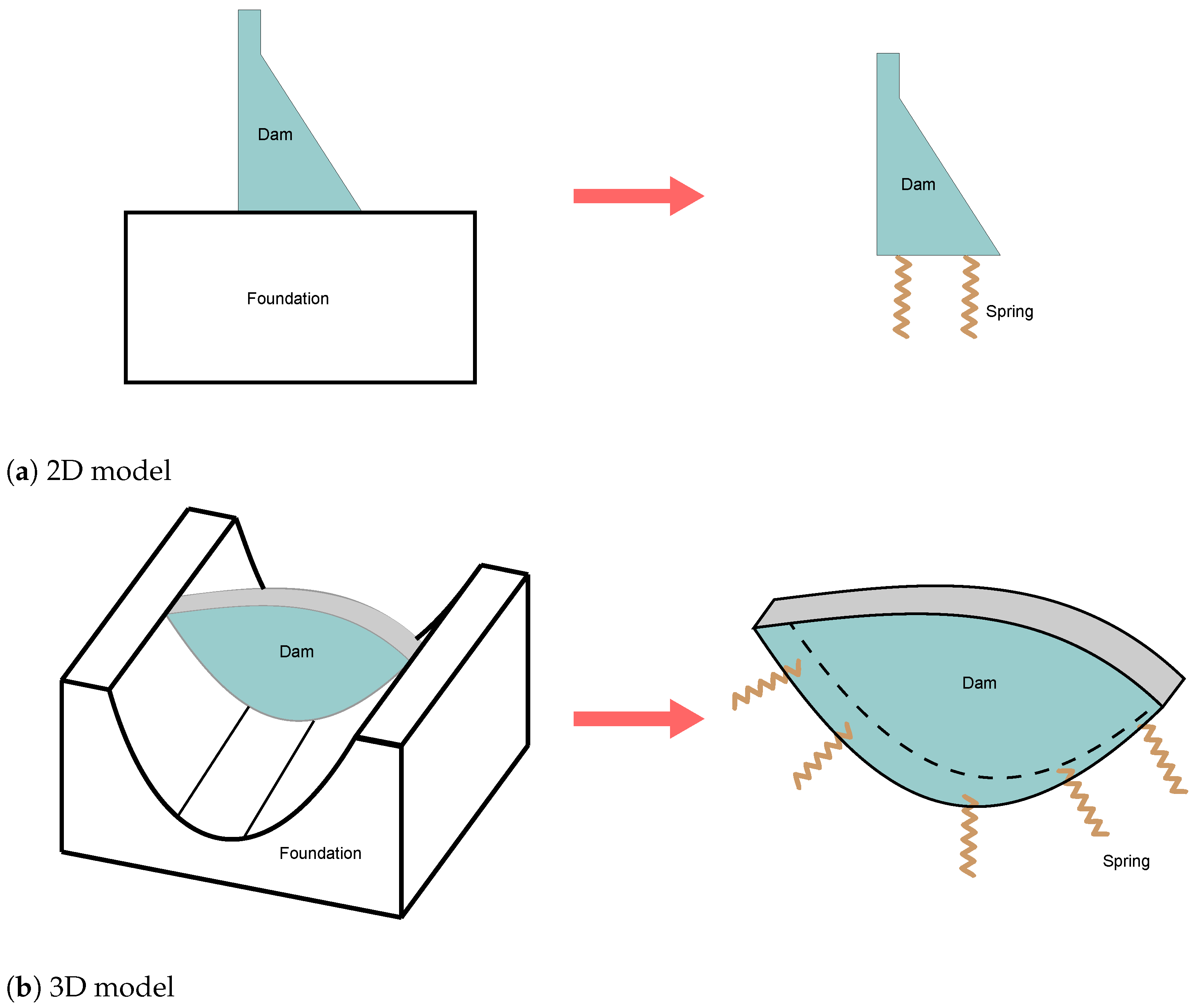
Figure 1. Simplified dam–foundation system using virtual springs for 2D and 3D models.
Water 16 02979 g001
Figure 2. Hierarchy of grey wolf (dominance decreases from top down).
Water 16 02979 g002
Figure 4. 2D FEM model of the gravity dam section.
Water 16 02979 g004
Figure 5. Positions of the measurement points in the gravity dam section.
Water 16 02979 g005
Figure 6. The deformation of the gravity dam under different water loads (unit: m).
Water 16 02979 g006
Figure 7. Results of deformation separation ( h w = 0.8 h d , unit: m).
Water 16 02979 g007
Figure 8. Results of deformation separation ( h w = h d , unit: m).
Water 16 02979 g008
Figure 9. FEM model of the arch dam.
Water 16 02979 g009
Figure 10. Layout of plumbs for the arch dam.
Water 16 02979 g010
Figure 11. Contour plot of downstream displacement distribution (unit: m).
Water 16 02979 g011
Figure 12. Contour plot of cross-stream displacement distribution (unit: m).
Water 16 02979 g012
Figure 13. Contour plot of vertical displacement distribution (unit: m).
Water 16 02979 g013
Figure 14. Layout of plumb for the arch dam, different colors represent different virtual springs.
Water 16 02979 g014
Figure 15. Distribution of measurement point errors (RE).
Water 16 02979 g015
Figure 16. RRMSE for different numbers of virtual springs.
Water 16 02979 g016
Figure 17. Dam material division diagram.
Water 16 02979 g017
Figure 18. Water level monitoring time history curve.
Water 16 02979 g018
Figure 19. Temperature monitoring time history curve.
Water 16 02979 g019
Figure 20. Displacements measured by some plumb lines.
Water 16 02979 g020
Figure 21. Optimisation process for the inversion of dam parameters.
Water 16 02979 g021
Table 1. Separation error of the 2D case.
PointDirection d c (m) d m (m)RE
AX 8.7438 × 10 3 8.7470 × 10 3 3.6379 × 10 4
Y 2.1532 × 10 3 2.1520 × 10 3 5.5050 × 10 4
BX 6.3472 × 10 3 6.3460 × 10 3 1.9025 × 10 4
Y 1.8904 × 10 3 1.8890 × 10 3 7.4020 × 10 4
CX 4.7841 × 10 3 4.7810 × 10 3 6.3267 × 10 4
Y 1.5878 × 10 3 1.5860 × 10 3 1.1711 × 10 3
DX 3.0515 × 10 3 3.0500 × 10 3 4.9403 × 10 4
Y 1.1404 × 10 3 1.1390 × 10 3 1.2509 × 10 3
EX 1.5254 × 10 3 1.5280 × 10 3 1.6788 × 10 3
Y 6.1503 × 10 4 6.2090 × 10 4 9.5454 × 10 3
Note: d c represents the calculated displacement, d m represents the measured displacement.
Table 2. Concrete material parameters.
Division ρ / ( Kg · m 3 ) c / [ KJ · ( Kg · k 1 ) ] λ / [ KJ · ( m · h · k ) 1 ] E/GPa
A25001.0478.47932.1
B25001.0568.22731.1
C25001.0728.01630.1
Table 3. Results of Young’s modulus inversion (unit: GPa).
PeriodABC
201639.5639.7337.95
201739.7240.0238.10
201839.6539.9638.10
Disclaimer/Publisher’s Note: The statements, opinions and data contained in all publications are solely those of the individual author(s) and contributor(s) and not of MDPI and/or the editor(s). MDPI and/or the editor(s) disclaim responsibility for any injury to people or property resulting from any ideas, methods, instructions or products referred to in the content.