Influence of Rainfall Patterns on Rainfall–Runoff Processes: Indices for the Quantification of Temporal Distribution of Rainfall

Abstract

To understand the influence of rainfall patterns on rainfall–runoff processes, we propose two indices: skewness_PEAK (skew_p), representing the relative timing of peak rainfall, and the normalized root-mean-square error peak (NRMSE_p), which quantifies the concentration of rainfall near the peak. By analyzing approximately 25,000 rainfall scenarios, we examined the relationship between these indices and peak flood discharge in the rainfall–runoff process. The analysis revealed that peak flood discharge positively correlates with the NRMSE_p, indicating that concentrated rainfall near the peak substantially increases discharge. Conversely, a negative correlation with skew_p suggests that earlier peak rainfall reduces discharge. These insights were synthesized into a three-dimensional solution space providing a comprehensive framework for predicting how variations in rainfall distribution affect flood discharge. The findings underscore the importance of incorporating these indices into real-time flood forecasting models and urban flood risk management strategies.

1. Introduction

The primary factors influencing rainfall–runoff processes are topography, soil, watershed characteristics, and rainfall properties [1,2,3]. Among these factors, rainfall considerably affects the hydrograph shape, peak flood discharge, and total discharge [4,5,6]. With the recent escalation in urban flooding risks due to climate change and poor planning, a deeper understanding of rainfall characteristics has become increasingly important. Previous research has primarily focused on estimating probable rainfall through frequency analysis, focusing primarily on the total amount of rainfall or its intensity [1]. However, the rise in flood damage caused by climate change is more closely associated with the concentration of floods caused by urbanization and the consequent increase in property damage, rather than a direct increase in rainfall itself.

The analysis of rainfall observation data generally does not reveal a significant upward trend over time in the annual maximum rainfall series [7,8]. Nonetheless, urban flood response policies often involve increasing design frequencies or introducing concepts such as target rainfall for disaster prevention, which effectively raise design rainfall standards [9,10,11]. For instance, measures are being implemented to extend the design frequency of storm sewers in urban areas from the existing 10–30 years to over 50 years [12], and to elevate the design frequency of small rivers to 200 years [13]. However, a series of studies has indicated that the effect of increasing the design frequency in domestic environments is limited. For example, when the design frequency was raised from a 50-year to 100-year frequency, the increase in the applied design rainfall was less than 10%, and the resulting flood discharge increase was approximately 15% [14]. To enhance flood defense capabilities in urban areas under such circumstances, it is crucial to consider the total rainfall as well as other characteristics such as the temporal distribution of rainfall.

A previous study has highlighted the significance of the temporal distribution of rainfall in the rainfall–runoff relationship [15]. Defined by terms such as intensity distribution, intensity profile, rainfall pattern, and rainfall temporal pattern, the temporal distribution refers to how the total rainfall is distributed over time [16]. This factor is critical as it directly influences flood discharge during the runoff process [17,18,19,20]. Despite its importance, research quantifying the temporal distribution of rainfall is relatively scarce compared to studies focusing on total rainfall.

Several methods have been developed to analyze the temporal distribution of rainfall. These include the Huff method [21], alternating block method, Mononobe method [22], and Yen and Chow method [23]. The method proposed by Yen and Chow [23] simplifies the hyetograph for design rainfall into a triangular shape and varies the peak rainfall time to occur in the early, middle, or late part of the rainfall event. Huff [21] developed a method using rainfall data in Illinois, USA, to express the relative timing of peak rainfall as a percentage of the total rainfall duration, wherein the time axis was divided into four quartiles. The alternating block method calculates the cumulative and segmental rainfall based on rainfall intensity for various durations (e.g., ∆t, 2∆t, and 3∆t) using the intensity–duration–frequency (IDF) curve. This method arranges the largest segmental rainfall amount at the center, alternating the subsequent largest amounts to the left and right. Similarly, the Mononobe method calculates cumulative rainfall over continuous durations and adjusts rainfall intensity using an empirical constant, n, but also provides an empirical formula for these calculations.

The Yen and Chow method and Huff method prioritize the relative position of the peak time on the hyetograph, whereas the alternating block method and Mononobe method emphasize the concentration of rainfall at the peak. These methods for analyzing the temporal distribution of rainfall primarily focus on two factors: the relative position of the peak time and the concentration of rainfall around the peak.

In previous research, various metrics have been developed to quantify the temporal distribution of rainfall. Oliver [24] introduced the precipitation concentration index (PCI), which measures the dispersion of monthly rainfall based on seasonal data: $\mathrm{PCI}=100\times \sum {{\mathrm{p}}_{\mathrm{i}}}^2/{(\sum {\mathrm{p}}_{\mathrm{i}})}^2$. A higher PCI indicates that annual rainfall is concentrated in a specific month, whereas a lower PCI, approaching ${\displaystyle \frac{100}{12}}$, suggests an even distribution across the year. Michiels et al. [25] refined the PCI by incorporating the coefficient of variance, standardizing the index to 100 for uniformly distributed monthly rainfall over the year: $\mathrm{PCI}=100/12\times [1+\left(\mathrm{s}/\overline{{\mathrm{p}}_{\mathrm{i}}}{)}^2\right]$. Thus, the PCI serves as a measure of annual rainfall concentration, highlighting variations in monthly precipitation. Máca and Torfs [6] proposed the R_max index, which quantifies the maximum rainfall ordinate to capture variations in the hyetograph according to temporal resolution. As the temporal resolution of the hyetograph decreases, the peak rainfall ordinate is diluted, leading to a lower R_max value. This index indirectly quantifies rainfall concentration by analyzing peak rainfall variations across different temporal resolutions.

Wartalska et al. [26] explored the correlation between hyetographs and drainage systems, proposing seven indices to quantify the temporal distribution of rainfall. These indices are categorized into two groups: two indices related to the peak rainfall time (r, the ratio of rainfall at the peak time to the duration of rainfall, and r_cg, the ratio of rainfall at the time when half of the total rainfall occurs) and five indices related to the overall rainfall distribution (M1, the ratio of rainfall before that after the peak time; M2, the ratio of maximum rainfall ordinate to total rainfall; and M3, M4, and M5, which measure the ratios of rainfall during the first third, 30%, and 50% of the rainfall duration, respectively, to the total rainfall). These indices provide a comprehensive framework for analyzing rainfall patterns in relation to drainage system performance.

Additionally, various algorithms for generating precipitation scenarios have been employed to apply the seven indices to the hyetograph, thereby quantifying its characteristics. The temporal distribution has been classified in greater detail than the traditional quartile-based distribution by Huff [21]. The seven indices introduced by Wartalska et al. [26] are designed to quantify the relative timing of peak rainfall. Concurrently, advancements in radar rainfall estimation technology have facilitated research into the spatial distribution of rainfall. Kim and Kim [27] investigated the effect of spatial resolution in grid-based radar rainfall on predicted flood discharge, employing the normalized root-mean-square error (NRMSE) formula ($\sqrt{{\displaystyle \frac{1}{\mathrm{n}}}\sum {({\displaystyle \frac{{\mathrm{p}}_{\mathrm{i}}-{\mathrm{p}}_{\mathrm{m}}}{{\mathrm{p}}_{\mathrm{m}}}})}^2}$)) to quantify the spatial variability of radar rainfall. This approach differs from that employed in previous studies by quantifying deviations in rainfall for spatial variability through the analysis of two-dimensional spatial distribution data, rather than using the ordinates of a hyetograph.

Previous studies on quantifying rainfall characteristics often overlooked the simultaneous consideration of two aspects: the relative timing of peak hours and the concentration of rainfall around these peaks, with an emphasis on the temporal distribution of rainfall. Therefore, here, we introduce a new index to quantify the temporal distribution of rainfall, focusing on the relative timing of the peak and the concentration of rainfall around it. The subsequent effect of the temporal distribution of rainfall on flood discharge in rainfall–runoff processes is then examined. The quantification indices for the temporal distribution of rainfall are detailed in Section 2. The applications of these indices to over 25,000 rainfall scenarios are reviewed in Section 3. The variations in the peak flood discharge in rainfall–runoff processes based on the distribution of rainfall duration using these indices are discussed in Section 4. The conclusions of this study are summarized in Section 5.

2. Quantification Indices for the Temporal Distribution of Rainfall

To quantify the relative timing of the peak, the skewness formula $\mathrm{E}[({\displaystyle \frac{\mathrm{X}-\mathsf{\mu }}{\mathsf{\sigma }}}{)}^3]$ was applied. Skewness is a measure indicating the asymmetry of a probability density function, which quantifies the extent to which a data distribution is skewed in a specific direction relative to its mean. We propose a modified skewness formula for the peak ordinate, showing that the distribution of the ordinate in the hyetograph resembles a probability density function. The modified skewness is expressed through a transformed third-moment equation:

$${\mathrm{skewness}}_{\mathrm{PEAK}}={\displaystyle \frac{1}{\mathrm{N}}}{{\displaystyle \sum }}_{\mathrm{j}=1}^{\mathrm{N}}({\displaystyle \frac{1}{\mathrm{n}-1}}{{\displaystyle \sum }}_{\mathrm{i}=1}^{\mathrm{n}}{({\displaystyle \frac{{\mathrm{t}}_{\mathrm{i}}-{\mathrm{t}}_{\mathrm{PEAK}}}{\mathrm{T}}})}^3)$$

(1)

where N denotes the ordinate number corresponding to the peak rainfall, n denotes the ordinate number of the hyetograph, t indicates time, t_PEAK denotes the peak time, and T indicates the rainfall duration.

Skewness_PEAK (hereinafter referred to as skew_p) is a metric designed to quantify the relative position of the peak time within the duration of rainfall. Skew_p is normalized and theoretically ranges from −0.25 to 0.25, irrespective of the rainfall duration (Figure 1). A skew_p value of 0 indicates that the peak time is at the midpoint of the rainfall duration. If the peak occurs at the beginning of the rainfall duration (i.e., within the first quartile), skew_p approaches 0.25. Conversely, if the peak is near the end of the rainfall duration (in the fourth quartile), skew_p approaches −0.25.

To quantify the concentration of rainfall around its peak relative to the total rainfall, the following equation for the normalized root-mean-square error (NRMSE) based on the peak was proposed:

$${\mathrm{NRMSE}}_{\mathrm{peak}}=\sqrt{{\displaystyle \frac{1}{\mathrm{n}-1}}{{\displaystyle \sum }}_{\mathrm{i}=1}^{\mathrm{n}}{({\displaystyle \frac{{\mathrm{p}}_{\mathrm{i}}-{\mathrm{p}}_{\mathrm{peak}}}{\mathrm{P}}})}^2}$$

(2)

where n denotes the ordinate number of the hyetograph, p_peak indicates the peak rainfall, P represents the total rainfall, and p_i represents the rainfall by the ordinate.

We applied the NRMSE method, as used by Kim and Kim [27], to analyze the spatial variability of rainfall through hyetographs and quantify the deviation of rainfall amounts by the ordinate based on peak rainfall. The resulting index, the NRMSE_peak (hereinafter referred to as the NRMSE_p), is normalized to the total rainfall and ranges from 0 to 1, regardless of the rainfall amount (Figure 2). When rainfall is uniformly distributed across all ordinates (i.e., when the rainfall intensity is constant throughout the event), the NRMSE_p is 0. As rainfall becomes more concentrated at a specific ordinate, the NRMSE_p increases. In cases where the total rainfall is concentrated at a single ordinate, the NRMSE_p reaches 1.

Skew_p and the NRMSE_p, as presented in this study, are independent indices that quantify the relative position of the peak time on the hyetograph and the concentration of rainfall around the peak relative to the total rainfall, respectively. These indices are not correlated with each other. Moreover, their normalization facilitates consistent comparisons of characteristics across various hyetographs, independent of factors such as rainfall duration, time intervals, and total rainfall amounts.

3. Quantification of Temporal Distribution by Rainfall Scenario

3.1. Generation of Rainfall Scenario

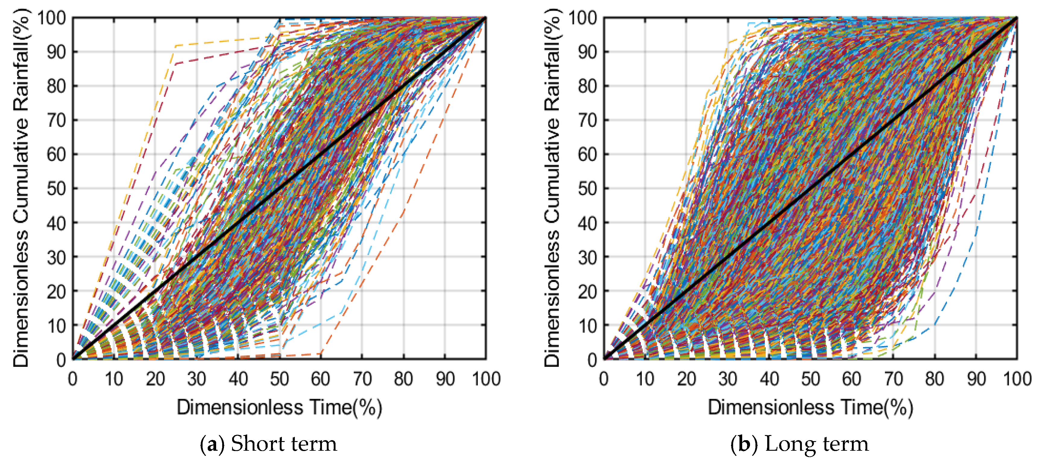
In this study, we developed a dimensionless cumulative rainfall scenario to capture the spatial and temporal characteristics of heavy rainfall events. The scenario was constructed using both historical observational data and future climate change projections to ensure reproducibility (Figure 3). This methodology aligns with approaches previously used in studies in China [15] and Germany [26]. The data employed in this research were obtained from the Korea Meteorological Administration’s Automated Synoptic Observation System (ASOS), covering the period from 1968 to 2022. We focused exclusively on instances of heavy rainfall (an alert criterion of the Korea Meteorological Administration), defined as over 60 mm within a 3 h period or over 20 mm within a 1 h period. Notably, during the 2022 flooding in Seoul’s Gangnam area, significant discrepancies in recorded rainfall values were observed between the ASOS Seoul Observatory (No. 108) and the AWS Gangnam Observatory (No. 400).

To address these regional differences, we also incorporated the d4PDF (database for policy decision making for future climate change) climate scenario. The d4PDF, developed by the Japanese Ministry of Education, Culture, Sports, Science and Technology, offers various ensemble scenarios for future climate policy decision making. It provides binary files with a spatial resolution of 20 km at hourly intervals (“https://diasjp.net (accessed on 1 September 2023)”). In our analysis, rainfall scenarios were generated for a duration of 12 h and categorized into short-term (<6 h) and medium-to-long-term (≥6 h) periods, resulting in 449 and 5789 scenarios, respectively (

Table 1. Summary of generated rainfall scenarios.

Rainfall Duration	Short Term (<6 h)		Long Term (≥6 h)
Data source	OBS	CCS	OBS	CCS
Number of scenarios	34	415	42	5747
Note	Primarily used in streams or medium-sized rivers		Primarily used in regional/large-sized rivers or national rivers

).

3.2. Distribution of Skew_p and NRMSE_p by Rainfall Scenario

To analyze the dimensionless cumulative rainfall distribution, we examined probable rainfall values for 50-, 80-, and 100-year return periods using hourly data from 68 ASOS stations (Figure 4) with over 30 years of records. We then applied the minimum (60.5 to 136.0 mm) and maximum (138.5 to 403.4 mm) probable rainfall values across durations of 60, 120, 180, 360, and 720 min.

In total, 12,925 hyetographs were generated, encompassing 449 short-term and 5789 long-term scenarios with durations ranging from 60 to 720 min. The relationship between skew_p and the NRMSE_p was analyzed for each hyetograph (Figure 5). The theoretical range for the NRMSE_p is between 0 and 1, but in this study, values were observed below 0.6, with a minimum of six rainfall ordinates. When rainfall intervals are constant, the NRMSE_p tends to be higher owing to a greater distribution of rainfall towards specific ordinates, especially when the duration is shorter, resulting in a smaller number of hyetograph ordinates.

The skewness of rainfall, skew_p, typically ranges between −0.25 and 0.25 during the rainfall event. For shorter durations, the limited number of ordinates restricts the possible peak locations, leading to a skewed distribution. Conversely, longer durations with more ordinates enable a more diverse placement of peaks, resulting in a more continuous distribution of skew_p values.

3.3. Comparison of Quantification Index with Conventional Huff Distribution

Using a reference duration of 180 min from 449 short-term rainfall scenarios, the distribution of rainfall durations in the newly generated scenarios was compared with the nationwide Huff percentile distributions reported by the Ministry of Land, Transport and Maritime Affairs (MLTMA) [28] and the Ministry of Environment [29]. The relative positions of the peak hours in the Huff quantiles were similar between the ministries. However, the Ministry of Environment’s [29] quantiles showed a greater concentration of rainfall at specific ordinates than those of the MLTMA [28], potentially because of the updated criteria for rainfall event selection as detailed in the “Development of Advanced Techniques for Korean Hydrological Analysis” [30]. These criteria include events with a daily rainfall of 30 mm or more, an hourly rainfall of 80 mm or more, or daily rainfall contributing to at least 10% of the annual total.

The Huff quantiles from both the MLTMA [28] and Ministry of the Environment [29] are categorized into four groups, corresponding to the traditional quartile-based approach, revealing distinct clusters of skew_p values (Figure 6). However, the rainfall scenarios in this study featured continuous peak occurrences in non-dimensional time, unlike the traditional quartile-based distribution. This led to increased diversity in peak occurrence locations compared to the previous rigid Huff quantiles, although there was a relative lack of rainfall concentration towards specific ordinates in the first and fourth quantiles compared to the overall rainfall. This observation suggests that while our method provides a broader view of potential peak occurrences, it may underrepresent certain extreme concentration patterns that are more typical in specific Huff quartiles, particularly in cases where peak rainfall occurs early or late in the event.

4. Change in Peak Flood Discharge of the Rainfall–Runoff Processes According to the Temporal Distribution of Rainfall

4.1. Selection of Target Areas and Rainfall–Runoff Simulation Method

To investigate the variations in peak flood discharge during rainfall–runoff processes, influenced by the temporal distribution of rainfall across different scenarios, 26 testbeds were selected (Figure 7). These areas were chosen based on the recent establishment of a river master plan and the availability of rainfall–runoff analysis data or easily accessible watershed characteristic factors and model parameters. The testbeds are distributed nationwide, with catchment areas ranging from 5.17 to 41.67 km², and have threshold durations between 3 and 12 h. Given these characteristics, scenarios for both short- and medium-to-long-term rainfall were established for analysis. This is particularly relevant considering recent flooding events caused by rainfall durations exceeding 6 h.

Under the River Act, for local rivers in a domestic context there is a requirement for the establishment or reassessment of a basic river plan every 10 years. During this process, flood discharge calculations for river planning are determined through rainfall–runoff simulations based on river design criteria [31]. This study adheres to these criteria, employing the Clark unit hydrograph method [32] for estimating flood discharge. The Clark unit hydrograph—a two-parameter model—utilizes travel time and a storage constant as parameters, which are determined using empirical formulas. Specifically, the travel time and hydraulic retention time were calculated using the continuous Kraven formula [33] and Sabol formula [34], respectively.

The Kraven (II) formula, foundational to the continuous Kraven formula, employs approximate values of average flow velocity (V) for each segment based on the average slope (S) and is commonly used in South Korea owing to its insensitivity to changes in S [35].

$${\mathrm{T}}_{\mathrm{c}}=16.667{\displaystyle \frac{\mathrm{L}}{\mathrm{V}}}$$

(3)

Steep slope (S > 3/400): $\mathrm{V}=4.592-{\displaystyle \frac{0.01194}{\mathrm{S}}}$, ${\mathrm{V}}_{\max }$ = 4.5 m/s;

Gentle slope (S ≤ 3/400): $\mathrm{V}=35,151.515{\mathrm{S}}^2-79.393939\mathrm{S}+1.6181818$, ${\mathrm{V}}_{\min }$ = 1.6 m/s.

$$\mathrm{K}={\displaystyle \frac{{\mathrm{T}}_{\mathrm{c}}}{1.46-0.0867\frac{{\mathrm{L}}^2}{\mathrm{A}}}}$$

(4)

where T_C denotes the arrival time (h), L indicates the channel length (km), V denotes the average flow velocity (m/s), S denotes the average slope, K indicates the retention constant (h), and A denotes the watershed area (km²). The Kraven (II) formula, which serves as the basis for the continuous Kraven formula, uses approximate V values for each segment of the average slope (S). It is widely used as a standard formula in South Korea owing to its advantage of being insensitive to S [35].

The infiltration condition was assessed using the NRCS curve number (or SCS curve number) method [36], with values directly adopted from the original river master plan. Given the relatively small watershed of the target areas ranging from 5.17 to 41.67 km², the base flow was not considered, reflecting the low population density in the area. The primary objective of this study was to analyze the pattern of variation in peak flood discharge relative to the distribution of rainfall duration. Therefore, the analysis assumes that there are no significant impediments to examining changes in flood discharge based on the set distribution of rainfall duration.

4.2. Relationship among skew_P, NRMSE_P, and Peak Flood Discharge

An analysis was conducted on the relationship among the NRMSE_p, skew_p, and peak flood discharge across 120 calculation points in 26 testbeds. The absolute values of peak flood discharge varied with the watershed characteristics at each calculation point. Despite these variations, the correlation between peak flood discharge and both the NRMSE_P and skew_p exhibited a consistent trend across all points. To analyze the variations in peak flood discharge in natural catchments relative to rainfall duration distribution, while controlling for differences in discharge magnitudes due to the catchment characteristics, the BW08 location was selected as the representative point. Additionally, the variations in peak flood discharge displayed a consistent pattern with the duration of rainfall, suggesting a normalized result for the duration of continuous rainfall in skew_p.

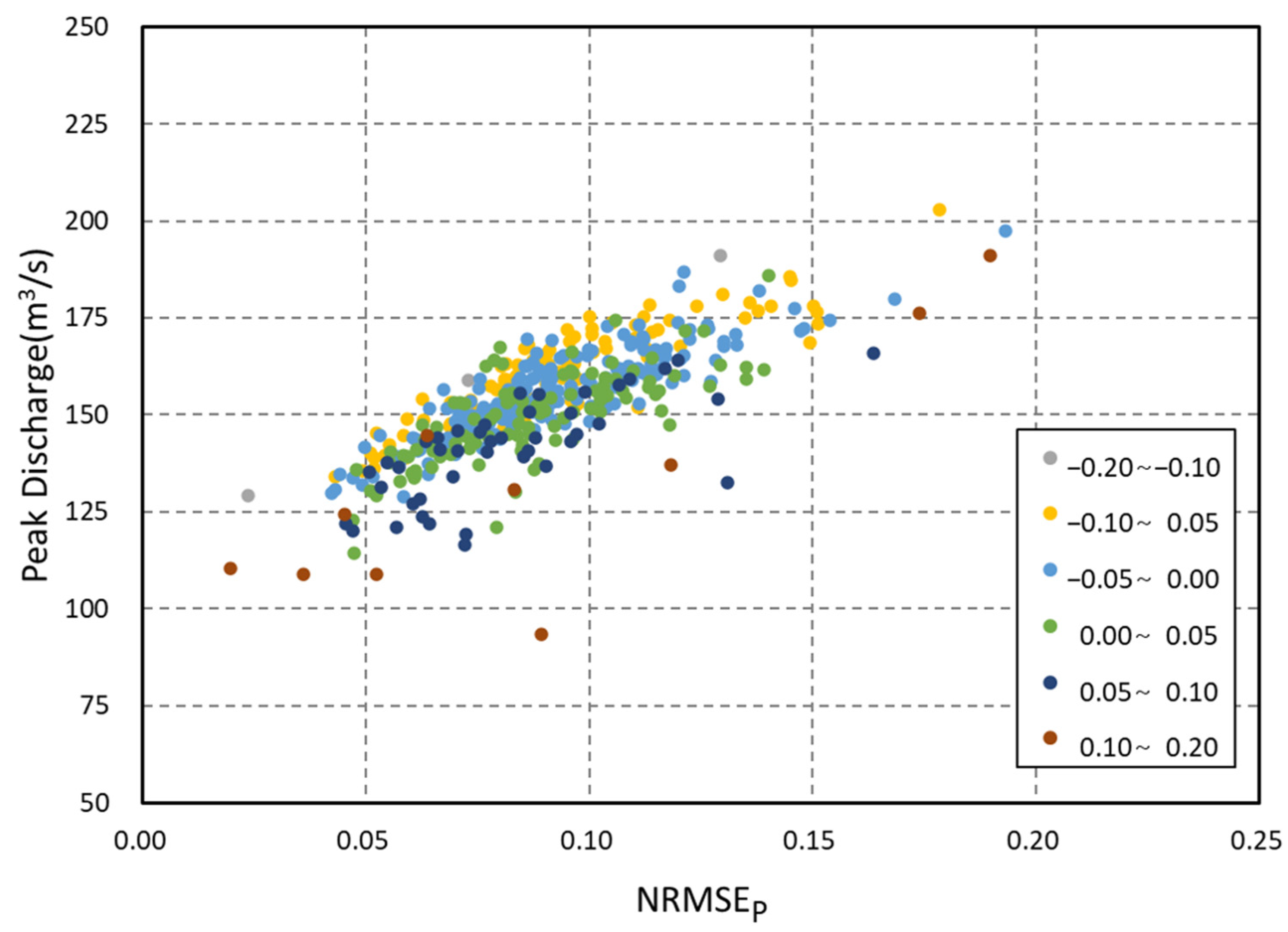
This study utilized a representative rainfall duration of 180 min to calculate peak flood discharge for 449 short-term rainfall scenarios at the BW08 location. The relationship between the NRMSE_p and peak flood discharge was examined for each hyetograph. To mitigate the influence of skew_p, it was categorized into equal intervals with a spacing of 0.05–0.1. The skewness classes in skew_p demonstrated a positive linear correlation with both the NRMSE_p and peak flood discharge (Figure 8,

Table 2. Linear regression between NRMSE_p and peak discharges.

Range of Skewp	Linear Regression	Correlation Coefficient
−0.20 to −0.10	Y = 584.06X + 115.82	1.00
−0.10 to −0.05	Y = 423.78X + 121.21	0.89
−0.05 to 0.00	Y = 408.25X + 118.29	0.87
0.00 to 0.05	Y = 398.51X + 114.94	0.74
0.05 to 0.10	Y = 368.41X + 110.98	0.71
0.10 to 0.20	Y = 452.45X + 93.12	0.84

). Specifically, as rainfall becomes more concentrated at a specific point relative to the total rainfall, the peak flood discharge in the rainfall–runoff relationship becomes significantly larger. This trend likely results from the direct effect of rainfall timing on peak flood discharge determination at the unit hydrograph.

The positive correlation between the NRMSE_p and peak flood discharge is analogous to the correlation between R_max, a variable quantifying rainfall concentration, and peak flood discharge as identified by Máca and Torfs [6]. Moreover, consistent correlations were observed between the finer spatial and temporal resolution of radar rainfall data, as presented by Kim and Kim [27], and an increase in peak runoff values.

To investigate the relationship between skew_p and peak flood discharge for each hyetograph, the NRMSE_p was categorized into intervals increasing by 0.02–0.06. A negative correlation between skew_p and peak flood discharge was observed when the NRMSE_p ranks were identical (Figure 9,

Table 3. Linear regression between skew_p and peak discharges.

Range of NRMSEp	Linear Regression	Correlation Coefficient
0.00 to 0.06	Y = −101.03X + 132.95	−0.70
0.06 to 0.08	Y = −94.53X + 145.12	−0.50
0.08 to 0.10	Y = −103.87X + 152.92	−0.52
0.10 to 0.12	Y = −102.45X + 161.07	−0.56
0.12 to 0.14	Y = −176.56X + 165.08	−0.77
0.14 to 0.20	Y = −11.10X + 179.77	−0.07

). This finding suggests that as the peak time of the hyetograph shifts from the fourth quartile to the first quartile, the flood discharge diminishes. In the SCS method for calculating effective rainfall, it is observed that the initial loss caused by the infiltration, termed initial loss ${\mathrm{I}}_{\mathrm{a}}$, is considerably higher when the peak of the hyetograph occurs earlier. This observation explains the aforementioned results.

5. Conclusions

Here, we introduced a method to quantify the effect of the temporal distribution of rainfall characteristics, beyond total rainfall, to enhance urban flood resilience in the context of climate change. To assess the effect of the temporal distribution of the rainfall on the peak flood discharge in rainfall–runoff processes, two indices were developed to measure the relative position of the peak time and the concentration of rainfall around the peak. These indices were employed to explore how the temporal distribution of rainfall affects peak flood discharge. To this end, approximately 25,000 rainfall scenarios were generated, and using the proposed indices, a comparative analysis was performed with the established design criterion of the Huff distribution. The scenarios confirmed a broader range of rainfall patterns concerning the timing and intensity of peak rainfall.

The analysis revealed that skew_p, which indicates the relative position of the peak time, negatively correlates with peak flood discharge, whereas the NRMSE_p, which measures rainfall concentration, positively correlates with peak flood discharge. A three-dimensional solution space was constructed to simultaneously consider the relationship between the two quantification indices and the normalized peak flood discharge by their mean (Figure 10). This solution space facilitates tracking variations in peak flood discharge across different rainfall duration distributions for a specified total rainfall. Given that flood discharge calculations for all domestic rivers are available, it is feasible to compute the relative flood discharge predicted based on the design flood discharge by determining the relative positions of the quantification indices for the design rainfall (Huff third quartile) and the specific index for the temporal distribution of rainfall. This approach can be directly applied to real-time flood forecasting for short-term precipitation and urban flood risk management strategies, particularly in the face of climate change-driven hydrological challenges. Furthermore, it is expected to provide essential foundational data for a deeper understanding of the effect of rainfall’s temporal distribution on rainfall–runoff processes.

References

1. Chow, V.T.; Maidment, D.R.; Mays, L.W. Applied Hydrology; McGraw-Hill: New York, NY, USA, 1988. [Google Scholar]
2. Bras, R.L. Hydrology: An Introduction to Hydrologic Science; Addison-Wesley: Boston, MA, USA, 1990. [Google Scholar]
3. Tarboton, D.G. Rainfall-Runoff Processes; Utah State University: Logan, UT, USA, 2003. [Google Scholar]
4. Obled, C.; Wendling, J.; Beven, K. The sensitivity of hydrological models to spatial rainfall patterns: An evaluation using observed data. J. Hydrol. 1994, 159, 305–333. [Google Scholar] [CrossRef]
5. Segond, M.L.; Wheater, H.S.; Onof, C. The significance of spatial rainfall representation for flood runoff estimation: A numerical evaluation based on the Lee chatchment, UK. J. Hydrol. 2007, 347, 116–131. [Google Scholar] [CrossRef]
6. Máca, P.; Torfs, P. The influence of temporal rainfall distribution in the flood runoff modelling. Soil Water Res. 2009, 4, S102–S110. [Google Scholar] [CrossRef]
7. Oh, T.; Kim, M.; Moon, Y.; Ahn, J. An analysis of the characteristics in design rainfall according to the data periods. J. Korean Soc. Hazard. Mitigat. 2009, 9, 115–127. (In Korean) [Google Scholar]
8. Kim, S.U.; Lee, Y.S. Flood frequency analysis considering probability distribution and return period under non-stationary condition. J. Korea Water Resour. Assoc. 2015, 48, 567–579. (In Korean) [Google Scholar] [CrossRef]
9. Ministry of the Interior and Safety (MOIS). Establishment Disaster Prev. Perform. Targets Reg. Considering Clim. Change Eff.; MOIS: Sejong-si, Republic of Korea, 2017. (In Korean)
10. Ministry of the Interior and Safety (MOIS). Establishment Disaster Prev. Perform. Targets Reg.; MOIS: Sejong-si, Republic of Korea, 2022. (In Korean)
11. Lenderink, G.; Buishand, A.; van Deursen, W.P.A. Estimates of future discharges of the river Rhine using two scenario methodologies: Direct versus delta approach. Hydrol. Earth Syst. Sci. 2007, 11, 1145–1159. [Google Scholar] [CrossRef]
12. Korea Water and Wastewater Works Association (KWWA). Drainage Sewer Design Guideline; KWWA: Seoul, Republic of Korea, 2022. (In Korean) [Google Scholar]
13. Ministry of the Interior and Safety (MOIS). Small Stream Design Guideline; MOIS: Sejong-si, Republic of Korea, 2024. (In Korean)
14. Jeong, J.; Kim, J. Improved practical methods for considering climate change in design flood estimation. J. Korean Soc. Hazard Mitig. 2022, 22, 301–309. (In Korean) [Google Scholar] [CrossRef]
15. Wang, F. Temporal pattern analysis of local rainstorm events in China during the flood season based on time series clustering. Water 2020, 12, 725. [Google Scholar] [CrossRef]
16. Dunkerley, D. The importance of incorporating rain intensity profiles in rainfall simulation studies of infiltration, runoff production, soil erosion, and related land surface processes. J. Hydrol. 2021, 603, 126834. [Google Scholar] [CrossRef]
17. Bell, V.A.; Moore, R.J. The sensitivity of catchment runoff models to rainfall data at different spatial scales. Hydrol. Earth Syst. Sci. 2000, 4, 653–667. [Google Scholar] [CrossRef]
18. Gires, A.; Onof, C.; Maksimovic, C.; Schertzer, D.; Tchiguirinskaia, I.; Simoes, N. Quantifying the impact of small scale unmeasured rainfall variability on urban runoff through multifractal downscaling: A case study. J. Hydrol. 2012, 442–443, 117–128. [Google Scholar] [CrossRef]
19. Bruni, G.; Reinoso, R.; van de Giesen, N.C.; Clemens, F.H.L.R.; ten Veldhuis, J.A.E. On the sensitivity of urban hydrodynamic modelling to rainfall spatial and temporal resolution. Hydrol. Earth Syst. Sci. 2015, 19, 691–709. [Google Scholar] [CrossRef]
20. Yuan, W.; Liu, M.; Wan, F. Study on the impact of rainfall pattern in small watersheds on rainfall warning index of flash flood event. Nat. Hazards 2019, 97, 665–682. [Google Scholar] [CrossRef]
21. Huff, F.A. Time distribution of rainfall in heavy storms. Water Resour. Res. 1967, 3, 1007–1019. [Google Scholar] [CrossRef]
22. Jeong, J.; Yoon, Y. Design Practices for Water Resources, 2nd ed.; Goomi Press: Seoul, Republic of Korea, 2007. [Google Scholar]
23. Yen, B.C.; Chow, V.T. Design hyetographs for small drainage structures. J. Hydr. Div. 1980, 106, 1055–1076. [Google Scholar] [CrossRef]
24. Oliver, J.E. Monthly precipitation distribution: A comparative index. Prof. Geogr. 1980, 32, 300–309. [Google Scholar] [CrossRef]
25. Michiels, P.; Gabriels, D.; Hartmann, R. Using the seasonal and temporal precipitation concentration index for characterizing the monthly rainfall distribution in Spain. Catena 1992, 19, 43–58. [Google Scholar] [CrossRef]
26. Wartalska, K.; Kaźmierczak, B.; Nowakowska, M.; Kotowski, A. Analysis of hyetographs for drainage system modeling. Water 2020, 12, 149. [Google Scholar] [CrossRef]
27. Kim, C.; Kim, D.H. Effects of rainfall spatial distribution on the relationship between rainfall spatiotemporal resolution and runoff prediction accuracy. Water 2020, 12, 846. [Google Scholar] [CrossRef]
28. Ministry of Land, Transport and Maritime Affairs (MLTMA). Improvement and Supplement of Probability Rainfall in South Korea; MLTMA: Sejong City, Republic of Korea, 2011. (In Korean) [Google Scholar]
29. Ministry of Environment. Standard Guideline for Design Flood; Ministry of Environment: Sejong, Republic of Korea, 2019. (In Korean)
30. Ministry of Land, Infrastructure and Transport (MOLIT). Development of Advanced Technology for Hydrologic Analysis in Korea; MOLIT: Sejong, Republic of Korea, 2017. (In Korean)
31. Korea Water Resources Association (KWRA). River Design Guideline and Commentary; KWRA: Daejeon, Republic of Korea, 2019. (In Korean) [Google Scholar]
32. Clark, C.O. Storage and the unit hydrograph. Trans. Am. Soc. Civ. Eng. 1945, 110, 1419–1446. [Google Scholar] [CrossRef]
33. Ministry of Land, Transport and Maritime Affairs (MLTMA). Design Flood Estimation Guide; MLTMA: Sejong City, Republic of Korea, 2012. (In Korean) [Google Scholar]
34. Sabol, G.V.; Unit, C. Clark Unit Hydrograph and R-parameter estimation. J. Hydraul. Eng. 1988, 114, 103–111. [Google Scholar] [CrossRef]
35. Yoo, C.S. A theoretical review of basin storage coefficient and concentration time using the Nash model. J. Korea Water Resour. Assoc. 2009, 42, 235–246. (In Korean) [Google Scholar] [CrossRef]
36. Soil Conservation Service (SCS), Chapter 10; Soil Conservation Service. Hydrology. In National Engineering Handbook; United States Department of Agriculture: Washington, DC, USA, 1956; Section 4, Supplement A.
Figure 1. Range of skewP value depending on hyetographs.
Water 16 02904 g001
Figure 2. Range of NRMSEp value depending on hyetographs.
Water 16 02904 g002
Figure 3. Dimensionless cumulative rainfall depth curves based on rainfall scenario.
Water 16 02904 g003
Figure 4. Spatial distribution of ASOS stations by the Korea Meteorological Administration across the Korean peninsula.
Water 16 02904 g004
Figure 5. Relationships between NRMSEP and skewP depending on rainfall scenarios.
Water 16 02904 g005
Figure 6. Comparison of rainfall scenarios and previous Huff distributions using NRMSEP and skewP [28,29].
Water 16 02904 g006
Figure 7. Location map of testbed and spatial distribution of flood estimation points.
Water 16 02904 g007
Figure 8. Positive relationships between NRMSEP and peak discharges.
Water 16 02904 g008
Figure 9. Negative relationships between skewp and peak discharges.
Water 16 02904 g009
Figure 10. Three-dimensional solution space between quantifying index for temporal distribution of rainfall and normalized peak discharge from rainfall–runoff process.
Water 16 02904 g010