Heterogeneous Interaction Effects of Environmental and Economic Factors on Green Efficiency of Water Resources in China

Abstract

Identifying the green efficiency of water resources and its driving factors is paramount for promoting sustainable development in China. The existing research has primarily focused on the spatial heterogeneity of individual factors that impact green efficiency of water resources. However, it has often overlooked the heterogeneity in the interactions between these factors. In this study, we utilized a multiscale geographically weighted regression (MGWR) model to discern the spatial heterogeneity of the individual factors influencing the green efficiency of water resources in China between 2002 and 2016. Subsequently, we demarcated several subregions based on the coefficients derived from the MGWR model. Employing a geographical detector (GD), we quantified the interactive impacts of different factors within these subregions. Our findings unveiled, for the first time, the diverse patterns in the temporal and spatial fluctuations in the factors impacting the eco-friendliness of water resources. The findings underscored that disregarding the spatial heterogeneity of these interactive effects may result in an underestimation of the interactions among factors. Significantly, in 2016, the impact of tertiary industry proportion and completed investment in pollution treatment displayed an enhanced non-linear effect across the entire sample and concurrently demonstrated a bivariate enhanced effect within subregions. These discoveries contribute to a deeper comprehension of the mechanisms influencing these factors, providing valuable insights for policymakers in crafting region-specific water resource policies tailored to the unique developmental requirements of different areas.

1. Introduction

Water, as a fundamental prerequisite for human survival and development, stands as an irreplaceable natural resource that is essential for maintaining the Earth’s ecosystem functions and supporting social and economic progress [1]. The current water resources cannot address the challenges brought about by global climate change, rapid population growth, and urban expansion. Forecasts suggest that over half of the world’s countries and regions will likely face water shortages [2]. The severity of water resource challenges is notably escalating in China, as evidenced by various studies [3,4,5]. Insufficient per capita allocation of water resources, coupled with uneven spatial and temporal distribution, underscores the gravity of the situation [6,7]. Furthermore, the issue is exacerbated by severe water pollution and inefficient water resource utilization [8,9]. Therefore, it is crucial to effectively and sustainably manage water resources. Exploring the factors influencing the green efficiency of water resources emerges not only as a direct and effective strategy to enhance utilization efficiency but also holds significant implications for effective carbon emission control and high-level environmental protection. In navigating the complexities of water resource challenges, understanding these factors becomes a crucial step toward fostering more responsible and sustainable water resource practices.

Research into the determinants of the green efficiency of water resources has predominantly concentrated on factors such as environmental regulations, economic levels, and industrial structure, as highlighted by recent studies [10,11,12]. Ding et al. argued that economic status negatively affects water resource efficiency, primarily driven by the presence of heavy industries characterized by substantial water and energy consumption. While these industries contribute significantly to economic growth, they also present challenges such as extensive pollution discharge and low efficiency of resource utilization [13]. Along a similar vein, Zhang et al. investigated the factors affecting industrial the green efficiency of water resources on a national scale and determined that industrial structure and urbanization exert a negative inhibitory effect [14]. Researchers have utilized a variety of approaches to investigate the elements influencing regional variations in the eco-friendliness of water resources. For example, Wang et al. applied the Tobit model to examine pertinent factors, considering the spatiotemporal distribution of industrial utilization across different provinces and cities within the Yangtze River Economic Belt [15].

The association between the green efficiency of water resources and its influencing factors exhibits prevalent spatial heterogeneity. Scholars recognize geographically weighted regression (GWR) as a promising approach for addressing spatial variation. This method distinguishes itself from the conventional ordinary least squares (OLS) model [16,17,18]. GWR has gained widespread acceptance among researchers globally for investigating the factors influencing the green efficiency of water resources [19]. While GWR facilitates the quantitative analysis of spatial heterogeneity, it uses a single kernel bandwidth for model applications. This limitation restricts its ability to capture diverse geographical processes across different spatial scales [20,21]. Taking into account that the modeling relationship between the green efficiency of water resources and its influencing factors often exhibits spatial differences at various scales, a multiscale geographically weighted regression (MGWR) model was introduced. This extension of the GWR model accommodates local or regional variations in the relationships between the response variable and the relevant covariates. By accounting for spatial heterogeneity and operational scale, the MGWR model facilitates the exploration of various influencing factors and their corresponding processes [22]. Moreover, considering the potential interactive effects among the drivers, a notable gap in understanding exists, particularly regarding the impact on the green efficiency of water resources, despite efforts in fields such as environmental science [23] and health science [24].

This paper presents an innovative approach, distinguishing itself from prior methods by quantifying the spatial variability in the diverse factors influencing green efficiency in water resource management. Our investigation delves into the temporal and spatial patterns, examining the evolving trends in the green efficiency of water resources alongside societal drivers. We integrate the interplay between societal influences and multiscale spatial effects, enriching our analysis comprehensively. Primarily utilizing the MGWR model, we scrutinize the spatial diversity in the socioeconomic, environmental, and technological factors impacting the green efficiency of water resources. Leveraging model coefficients, we delineate the study area into distinct subregions and employ a GD model to uncover interactions among these driving factors within each subregion. Notably, this study is the first to reveal the spatial disparities in interactions among the driving factors of the green efficiency of water resources. The overarching goal of this research is to furnish governmental decision-making bodies with empirical references and scientific foundations for formulating more efficacious strategies to augment the green efficiency of water resources.

2. Materials and Methods

2.1. The Green Efficiency of Water Resources

We utilized the slacks-based measure–data envelopment analysis (SBM-DEA) model, developed by Tone [25], to assess the green efficiency of water resources in China. The traditional DEA model overlooks the economic benefits lost due to unintended outputs and fails to account for slack between inputs and outputs [26]. In contrast, the SBM-DEA model directly integrates the slack variables for each input and output into the objective function. This integration yields a more precise green efficiency value for the water resources of each decision-making unit [27,28,29]. The model is as follows:

$$\delta =\min {\displaystyle \frac{1-\frac{1}{N}{{\displaystyle \sum }}_{n=1}^N{S}_n^x/x_{k^{\prime }n}^{t^{\prime }}}{1+\frac{1}{M+H}\left({{\displaystyle \sum }}_{m=1}^M\frac{S_m^y}{y_{k^{\prime }m}^{t^{\prime }}}+{{\displaystyle \sum }}_{h=1}^H\frac{S_h^b}{y_{k^{\prime }h}^{t^{\prime }}}\right)}}$$

(1)

$$s.t.{{\displaystyle \sum }}_{t=1}^T{{\displaystyle \sum }}_{k=1}^K{\lambda }_k^t{x}_{kn}^t+S_n^x=y_{k^{\prime }n}^{t^{\prime }},n=1,\dots , N$$

(2)

$${{\displaystyle \sum }}_{t=1}^T{{\displaystyle \sum }}_{k=1}^K{\lambda }_k^t{y}_{km}^t-S_m^y=y_{k^{\prime }m}^{t^{\prime }}m=1,\dots , M$$

(3)

$${{\displaystyle \sum }}_{t=1}^T{{\displaystyle \sum }}_{k=1}^K{\lambda }_k^t{b}_{kh}^t+S_h^b=b_{k^{\prime }h}^{t^{\prime }}h=1,\dots , H$$

(4)

$${\lambda }_k^t\ge 0, S_n^x\ge 0, S_m^y\ge 0, S_h^b\ge 0,k=1,\dots , K$$

(5)

where $\delta$, $N$, $M$, $H$, and $K$ denote the green efficiency of water resources, the number of input types, the number of expected output types, and the number of unexpected output types, respectively. Meanwhile, $x$, $y,$ and $b$ represent the input, expected output, and unexpected output vectors, respectively. $S_n^x$ represents the input redundancy, while $S_h^b$ represents the unexpected output redundancy. $S_m^y$ indicates the expected output deficiency. $\left(x_{k^{\prime }n}^{t^{\prime }}, y_{k^{\prime }m}^{t^{\prime }}, y_{k^{\prime }h}^{t^{\prime }}\right)$ represents the first $k^{\prime }$ input–output values of production unit $t^{\prime }$, and ${\lambda }_k^t$ is the weight of the decision-making unit. The $\delta$ objective function is strictly monotonically decreasing on $S_n^x$, $S_m^y$, and $S_h^b$, with $0<\delta \le 1$. The evaluated decision-making unit is effective, and there is no input or output redundancy or deficiency when $\delta =1$ and $S_n^x=S_m^y=S_h^b=0$.

2.2. Spatial Autocorrelation

The local Moran’s I index is frequently employed for the estimation and examination of spatial dependence and heterogeneity among entities in spatial autocorrelation analyses [30,31,32]. This index is employed for spatial autocorrelation and clustering analysis, providing insights into the similarities and differences in water resource efficiency among adjacent provinces [33,34]. The formula for the local Moran’s I statistic is as follows:

$$I_i={\displaystyle \frac{\left(x_i-\overline{x}\right)}{S^2}}{{\displaystyle \sum }}_{j=1}^n{w}_{ij}\left(x_i-\overline{x}\right)$$

(6)

$$\mathrm{s}={{\displaystyle \sum }}_{i=1}^n{{\displaystyle \sum }}_{j=1}^n{W}_{ij}$$

(7)

where $x_i$ represents the green efficiency of water resources of province i; $W_{ij}$ represents the spatial weight matrix, n is the number of provinces; $\overline{x}$ and $s$ represent the mean and standard deviation of $x_i$, respectively. $I_i$ is the local Moran’s I of province i. If $I_i$ is >0, it indicates a positive correlation between the green efficiency of water resources of province i and that of its neighboring provinces. If $I_i$ is <0, it indicates a negative correlation between the green efficiency of water resources of province i and that of its neighboring provinces.

The four clustering types signify distinct spatial relationships between the green efficiency of water resources and neighboring provinces. Within these clusters, high and low indicate the degree of correlation between the independent variable and the dependent variable, H-H (high-high) and L-L (low-low) demonstrate positive spatial autocorrelation, whereas L-H (low-high) and H-L (high-low) show negative spatial autocorrelation [32,35]. The delineation of these spatial clustering types emphasizes that the analysis of local spatial autocorrelation can unveil distinctive attributes of local spatial clustering [36,37,38,39,40].

2.3. Multiscale Geographically Weighted Regression

The OLS model is one of the most widely used estimation methods in linear regression analysis and is considered a global regression model [41,42,43]. We used the second half of the equation in the OLS model to reflect the overall statistical correlation between the dependent variable and multiple explanatory variables:

$$y_j={\beta }_0+{{\displaystyle \sum }}_{p=1}^t{\beta }_p{x}_{ip}+\epsilon$$

(8)

where $y_j$ is the dependent variable, β₀ is the intercept, ${\beta }_p$ refers to the estimated parameter of independent variable $x_{ip}$, t is the number of impact factors, and $\epsilon$ represents the error term.

In contrast to the OLS model, GWR stands out as a local spatial technique. It effectively addresses spatial nonstationarity by incorporating spatial location into the regression parameters [17,44]. However, the GWR model assumes that the scales of all pertinent relationships remain constant across space, preventing the analysis of these relationships at varying scales [44,45,46]. Consequently, the development of a methodology capable of exploring local spatial relationships among variables involved in different processes at distinct scales becomes imperative.

By optimizing the bandwidths for explanatory variables, the MGWR model notably enhances model performance, resulting in more accurate parameters compared to the GWR model [47]. Fine-tuning the bandwidths for explanatory variables in the MGWR model leads to a notable enhancement in the precision of regression analysis. This results in more accurate parameters compared to those obtained through GWR [48,49]. The MGWR is formulated as follows:

$$y_j={\beta }_{bw0}\left(u_j,v_j\right)+{{\displaystyle \sum }}_{k=1}^t{\beta }_{bwk}\left(u_j,v_j\right)x_{jk}+{\epsilon }_j$$

(9)

where the $bwk$ in ${\beta }_{bwk}$ indicates the bandwidth used for parameter estimates. The MGWR excels in providing a more precise depiction of spatial heterogeneity by considering the influence of various scales in the spatial process. In this context, the disparity in bandwidths reflects the distinction in spatial scales.

The adaptive bi-square kernel function was utilized to ascertain the optimal bandwidth, effectively mitigating the influence of observations beyond the specified bandwidth. This approach minimizes both the Akaike Information criterion (AIC) and the corrected AIC (AICc). Additionally, the performance of the MGWR and OLS models in explaining the green efficiency of water resources across China was compared. This comparison utilized metrics such as adjusted R² values, residual sum of squares (RSS), AIC, and AICc.

2.4. Geographical Detector Model

The GD model is a statistical approach used to detect spatially stratified heterogeneity and its influencing factors. It is commonly employed in research across various fields, including land use, ecology, and urban studies. The model suggests that if an independent variable (X) correlates with a dependent variable (Y), there is significant consistency in their spatial characteristics [50,51]. The GD model encompasses four types of detectors: factor, interaction, ecology, and risk detectors [52]. In this study, we used factor and interaction detectors to assess how variables and their interactions affect the green efficiency of water resources.

The GD model utilizes a q statistic in the factor detector to measure how variable X influences the spatial heterogeneity of variable Y. The q statistic is calculated as follows:

$$q=1-{\displaystyle \frac{{{\displaystyle \sum }}_{h=1}^L{N}_h{\sigma }_h^2}{N{\sigma }^2}}=1-{\displaystyle \frac{SSW}{SST}}$$

(10)

$$SSW={{\displaystyle \sum }}_{h=1}^L{N}_h{\sigma }_h^2$$

(11)

$$SST=N{\sigma }^2$$

(12)

where h = 1, 2,…, L represents a specific stratum of the explanatory variable X, L is the total number of strata, N is the number of samples in stratum h or the entire study area, and ${\sigma }_h^2$ and ${\sigma }^2$ are the variances of dependent variable Y in stratum h or the entire study area, respectively. The q-statistic value ranges between 0 and 1, with a higher value indicating a stronger association between the independent variable X and the dependent variable Y.

The interaction detector is designed to quantify the interactive effects of two explanatory variables, X1 and X2. It also clarifies whether the interaction between these variables enhances or diminishes their influence on Y. Initially, the q-statistic value of the two explanatory variables was computed after their interaction, q(X1∩X2). Following this, the newly calculated q-statistic value was compared to the original q-statistic values of the individual explanatory variables, q(X1) and q(X2). The interaction types encompass five categories (Appendix A): nonlinear weakened if q(X1∩X2) < Min(q(X1), q(X2)), univariate weakened if Min(q(X1), q(X2)) < q(X1∩X2) < Max(q(X1), q(X2)), independent if q(X1∩X2) = q(X1) + q(X2), bivariate enhanced if q(X1∩X2) > Max(q(X1), q(X2)), and nonlinear enhanced if q(X1∩X2) > q(X1) + q(X2). To explore interaction heterogeneity, this study also aimed to apply an interaction detector to various subregions. This was based on the positive and negative estimated coefficients obtained from the MGWR model.

2.5. Data Sources

Socioeconomic activities not only consume energy but also contribute to continuous damage to the water environment [53]. Therefore, strategies crucial for achieving harmonized and sustainable development across economic, social, and ecological domains include decreasing resource consumption, improving ecological governance, and prioritizing environmental protection [54]. Based on previous research, the influencing factors of the green efficiency of water resources can primarily be attributed to socioeconomic development, technological progress, and investments in environmental protection [11,55]. Aligned with these research discoveries, our investigation chose particular data points, encompassing GDP per capita, the share of the tertiary industry, population size, water consumption in industrial and agricultural sectors, total highway length, discharged chemical oxygen demand (COD), completed investment in pollution treatment, and turnover in the technology market (refer to

Table 1. Data source description.

Factor	Variable Description	Abbreviation	Spatial Resolution	Data Sources
Socioeconomic
Economic level	GDP per capita	GDP	Provincial level	China Statistical Yearbook (CSY)
Industrial structure	Proportion of tertiary industry	PTI	Provincial level	China Statistical Yearbook (CSY)
Population size	Population	PO	Provincial level	China Statistical Yearbook (CSY)
Water use structure	Industrial water consumption	IWC	Provincial level	China Statistical Yearbook (CSY)
	Agricultural water consumption	AWC	Provincial level	China Statistical Yearbook (CSY)
Transportation infrastructure	Total length of highways	TLH	Provincial level	China Statistical Yearbook (CSY)
Environment
Pollution degree	COD discharged	COD	Provincial level	China Statistical Yearbook (CSY)
Environmental protection input	Investment completed in pollution treatment	ICPT	Provincial level	China Statistical Yearbook (CSY)
Technology
Technology conversion rate	Technology market turnover	TMT	Provincial level	China Statistical Yearbook (CSY)

). The data for these nine socioeconomic, environmental, and technological factors were extracted from the China Statistical Yearbook (CSY) and China City Statistical Yearbook (CCSY) in 2002 and 2016.

3. Results

3.1. The Spatial Variation Characteristics of the Green Efficiency of Water Resources

We utilized the SBM-DEA model, which includes undesirable outputs, to evaluate the green efficiency of water resources in every province in China. For this study, the weight ratio of desirable to undesirable outputs in the SBM-DEA model was fixed at 1:1 to gauge the green efficiency of water resources with undesirable outputs.

As depicted in Figure 1, the regions exhibiting relatively higher green efficiency of water resources encompassed Beijing, Tianjin, Jiangsu, Hainan, Tibet, and Qinghai. This observation suggests that the overall water resource efficiency in the eastern coastal region surpasses that in the central region. Interestingly, we observed heightened green efficiency of water resources in economically less developed regions, suggesting that the degree of the green efficiency of water resources in a region may not necessarily align with its level of economic development. The efficiency demonstrated in the green efficiency of water resources signifies optimized inputs and outputs.

It is important to highlight that the efficiency value determined by DEA signifies the relative efficiency of inputs and outputs, rather than indicating the rate of water resource utilization. This clarification elucidates the effective water resource utilization efficiency observed in economically underdeveloped areas. Moreover, the success of the green efficiency of water resources in Qinghai, Tibet, and Inner Mongolia suggests a dedication in these areas to the effective utilization of water resources.

3.2. Spatial Agglomeration Features

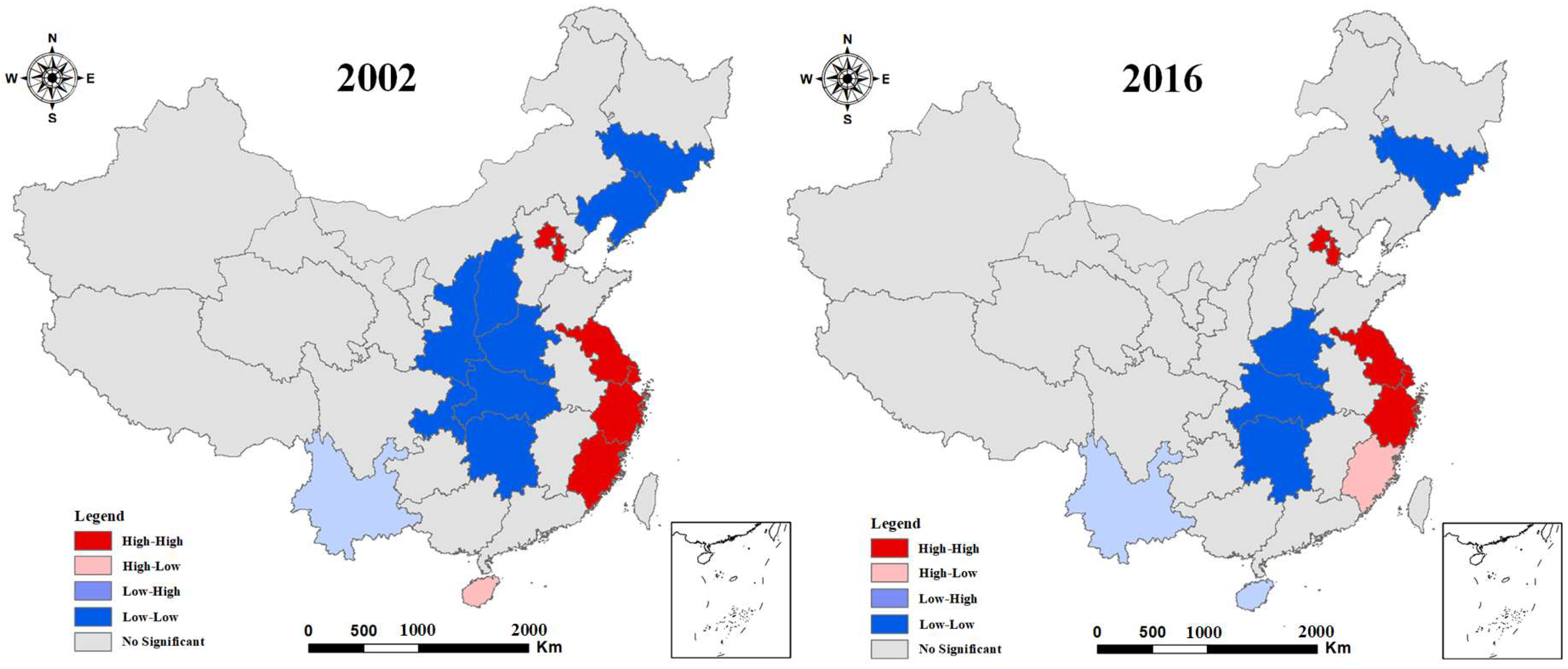
The spatial clustering of the green efficiency of water resources was examined using the local Moran’s I test. The local spatial autocorrelation index (LISA) was utilized to measure the degree of spatial autocorrelation in the green efficiency of water resources within the study area, revealing variations in spatial autocorrelation throughout the study period. The LISA cluster map spanning 2002 to 2016 predominantly featured H-H and L-L clustering, with the distribution of L-H and H-L clustering appearing relatively scattered and insignificantly concentrated (refer to Figure 2).

From 2002 to 2016, stable and highly concentrated regions with green efficient use of water resources were identified in North China, Jiangsu, Zhejiang, and Shanghai. The consistently high comprehensive green efficiency of water resources in this region during the study period can be attributed to factors such as a developed economic level, advanced technology, policy-driven regulations, and other contributing elements.

In 2002, the distribution of the green efficiency of water resources remained consistent within the L-L cluster region, primarily located in the central and northeast regions. By 2016, the clustering of L-L green efficiency of water resources in the provinces had diminished yet remained significant in major agricultural provinces such as Henan, Hubei, and Hunan. Environmental pollution intensification in the central region of China, owing to a lack of capital and technology, as well as lax regulatory policies, has contributed to a lower green efficiency of water resources. Additionally, the advantage of policies was not evident in these areas, further diminishing the green efficiency of water resources. Furthermore, the number of provinces displaying significant L-H and H-L clustering of the green efficiency of water resources was minimal and displayed a divergent distribution.

3.3. Global Driving Factors Influencing the Green Efficiency of Water Resources

The factors driving the green efficiency of water resources encompass socioeconomic, environmental, and technological variables. Using the stepwise regression method and correlation tests, we identified crucial determinants of the green efficiency of water resources from independent variables. These variables encompassed GDP per capita, the proportion of the tertiary industry, population, total length of highways, investment completed in pollution treatment, and technology market turnover. To gain a comprehensive understanding of the combined impact of various factors influencing the green efficiency of water resources in China, this study employed a global regression model to pinpoint the primary provincial drivers, where asterisks indicate the level of significance of the variable. Before delving into the OLS model results, we assessed the linear relationships between the various factors using the variance inflation factor (VIF). As shown in

Table 2. Global regression results.

Variable	2002		2016
	Coefficient	VIF	Coefficient	VIF
Intercept	9.195 **	2.372	9.631 *	1.799
GDP	−0.083 ***	1.508	0.005 ***	1.692
PTI	−0.594 ***	2.669	−0.060 ***	1.103
PO	0.011 ***	3.827	0.118 ***	1.042
TLH	0.008 **	1.467	0.025 ***	1.365
ICPT	0.040 ***	1.041	0.072 ***	1.052
TMT	0.001 ***	1.282	0.003 **	1.394

Notes: ***, **, and * indicate significance at the 1%, 5%, and 10% levels, respectively.

, multicollinearity was not a concern since the VIFs for all variables were well below 10, confirming a lack of significant multicollinearity in the model.

The OLS regression outcomes revealed that, in both 2002 and 2016, five explanatory variables demonstrated statistical significance at the 1% level. Notably, the significance level for the influence of TLH in 2002 and TMT in 2016 on the green efficiency of water resources was observed at 5%. The coefficients derived from the OLS model revealed that a majority of explanatory variables, such as PO, TLH, ICPT, and TMT, exhibited a positive correlation with the green efficiency of water resources. On the contrary, GDP and the PTI exhibited notably adverse impacts on the green efficiency of water resources.

3.4. Spatial Heterogeneity of the Influence of Driving Factors

Table 3. Comparison of model performance between the global OLS and the local MGWR models.

Models	R2	Adjusted R2	AIC	AICc	RSS
OLS-2002	0.643	0.618	585.424	599.136	84.250
MGWR-2002	0.807	0.772	520.003	527.804	61.459
OLS-2016	0.715	0.679	535.791	542.261	76.620
MGWR-2016	0.862	0.834	477.206	483.290	58.943

compares the efficacies of the OLS and MGWR models. The MGWR model demonstrated superior fit to the OLS model, as indicated by consistently higher R-squared and adjusted R-squared values over the entire study period. Additionally, the smaller AIC and AICc values in the MGWR model indicated a diminished disparity between the observed and fitted values, while a smaller RSS suggested reduced information loss in the model.

Table 4. Local estimates of MGWR model.

Variable	2002				2016
	Min	Max	Median	Bandwidth (km)	Min	Max	Median	Bandwidth (km)
Intercept	8.192	9.504	8.733	30	8.860	9.935	9.247	28
GDP	−0.213	0.119	−0.097	397	−0.182	0.298	0.011	383
PTI	−13.518	5.982	−0.682	418	−6.272	5.580	−0.142	402
PO	−0.414	0.258	0.003	365	−0.305	0.597	0.104	361
TLH	−0.040	0.026	0.002	493	−0.032	0.630	0.011	510
ICPT	−0.063	0.398	0.028	181	−0.031	0.484	0.062	166
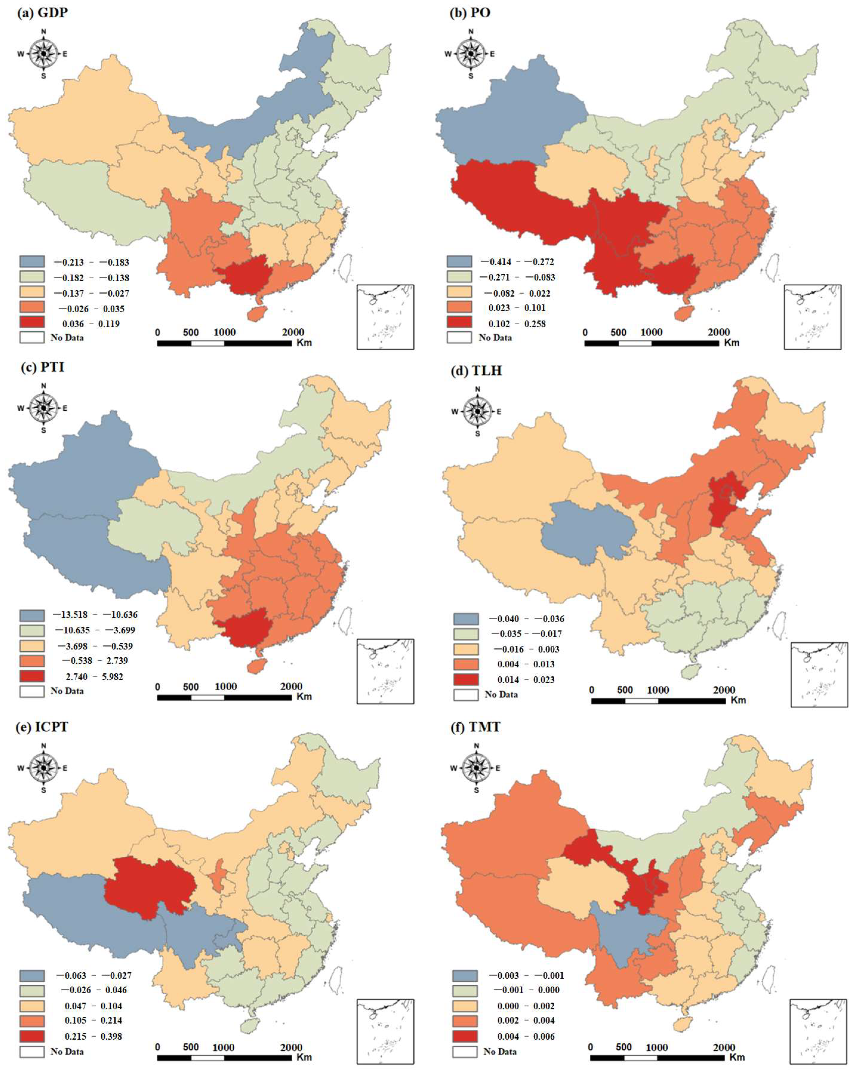
TMT	−0.005	0.006	−0.001	572	−0.003	0.006	0.002	549

furnishes a statistical overview of the local coefficients for each location in the MGWR model, revealing considerable variability in the impact of various factors on the green efficiency of water resources across different provinces. The values of all driving factors varied between positive and negative, indicating that the selected influencing factors exhibited significant spatial heterogeneity in their impact on the green efficiency of the water resources in China. To accurately depict the spatial variation in and influence of these influencing factors, Figure 3 and Figure 4 visually illustrate the spatial distribution of the local coefficients from 2002 to 2016.

Figure 3a and Figure 4a illustrate the evolving impact of per capita GDP on the green efficiency of water resources throughout the study period, transitioning from a north-to-south increasing trend to a scattered distribution. While the regions with positive per capita GDP regression coefficients expanded, not all areas with elevated economic development demonstrated high efficiency. Conversely, the green efficiency of the water resources in regions with low levels of economic development surpassed that in some developed eastern regions, emphasizing that the level of economic development was not the sole determinant of the green efficiency of water resources. Figure 3b and Figure 4b illustrate the regions with minimal alteration in the positive coefficient of population size in China between 2002 and 2016, predominantly found in thinly populated areas in the western region. This implies that population growth had a promotive impact on specific thinly populated areas in the western region, but, in the majority of regions, population expansion did not contribute to enhancing the green efficiency of water resources. Therefore, provinces should formulate and implement population policies tailored to local development conditions to mitigate the inhibitory effect of population size on the green efficiency of water resources.

Figure 3c and Figure 4c illustrate the growing influence of the proportion of tertiary industry on the green efficiency of the water resources across China, indicating a superior economic structure in the southeastern region compared to that in the northwestern region. Concerning adjusting the industrial structure, the northwestern region exhibits greater potential for adjustment than the southeastern region. Therefore, a conscious increase in the proportion of tertiary industries in the northwestern region, under similar conditions, could yield more benefits than in the southeastern region. Figure 3d and Figure 4d reveal that transportation infrastructure significantly influenced the green efficiency of the water resources. The count of regions with positive regression coefficients in the study area rose from 2002 to 2016, predominantly found in the eastern and central regions. This indicates that the development of transportation infrastructure contributed to improving the green efficiency of water resources. Notably, the level of infrastructure construction in the eastern and central regions was greater than that in the western region. Therefore, the western region should intensify the construction of transportation infrastructure to foster socioeconomic development and enhance the green efficiency of water resources.

Figure 3e and Figure 4e illustrate that the regression coefficients indicating the relationship between the degree of pollution and environmental protection investment in environmental factors were positive in the majority of the regions. This suggests that increasing investment in environmental pollution control helped improve the green efficiency of water resources. Figure 3f and Figure 4f illustrate that the impact of technological factors on the green efficiency of water resources primarily manifested through the impact of trading volume in the technology market. While the regression coefficient for turnover in the technology market was noticeably smaller than that for other factors, a substantial majority of regions demonstrated a positive trend. This suggests that advancements in the technology conversion rate played a significant role in improving the green efficiency of water resources. Therefore, regions should augment their investments in scientific research and prioritize the transformation of scientific research achievements to establish technology as a new focal point for advancing the green efficiency of water resources.

3.5. Spatial Heterogeneity of Interactions between Driving Factors

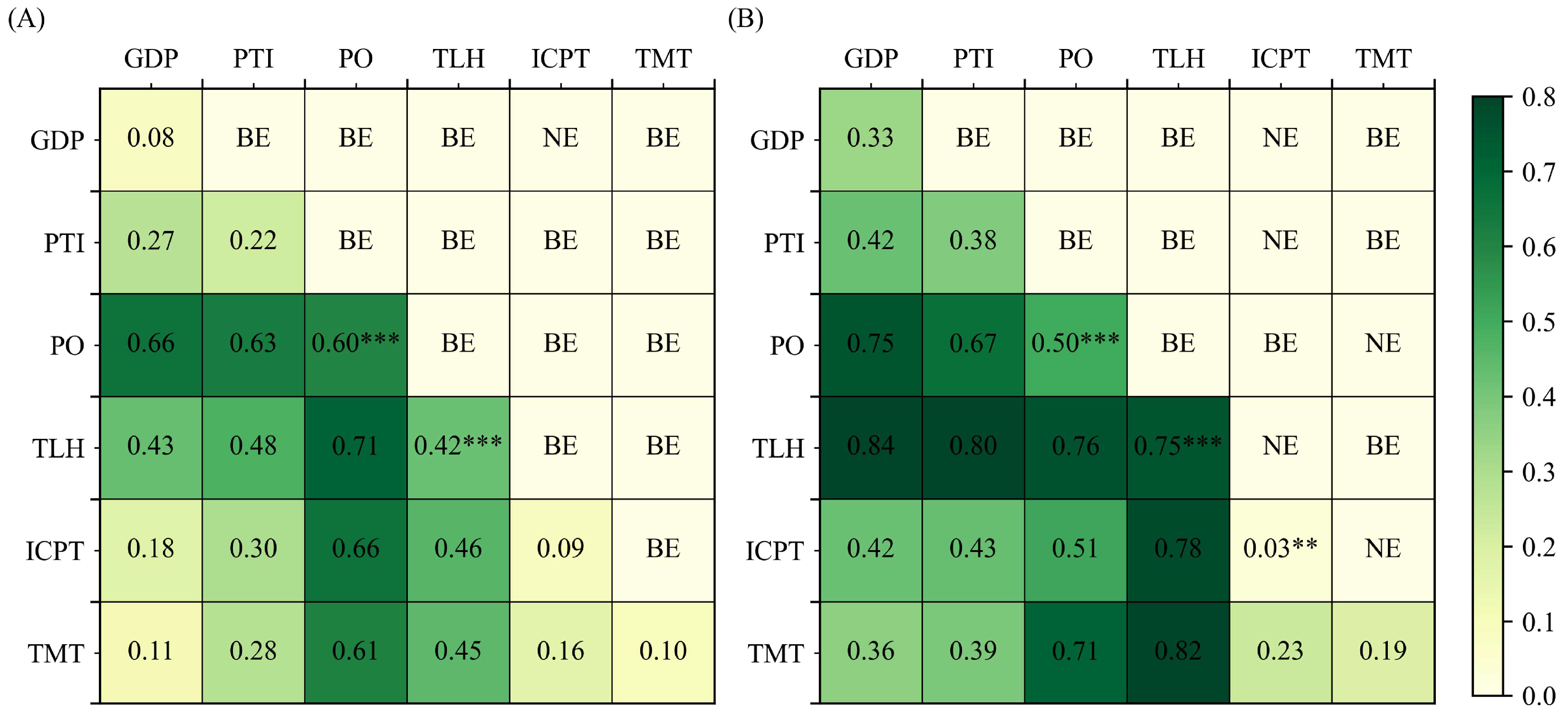
From 2002 to 2016, the q-statistic values of most variables increased (Figure 5). While the ICPT q-statistic value decreased, its significance level increased. These findings indicate that all variables had a higher impact on the green efficiency of the water resources in 2016. These results were also found for the interaction detectors. In 2002, only the interaction between GDP and ICPT enhanced nonlinearly; however, there were more nonlinear relationships among the variables in 2016. Regarding the different variables, PO and TLH had the highest q-statistic values at the set significance level (q-statistic values were 0.60 and 0.42, respectively), and their interactions with other variables were the highest. This suggests that these two variables played important roles in the green efficiency of water resources.

As previously stated, the diverse impacts of various factors can affect the outcomes of the interaction detector. In this study, we computed all interactions within the subregions. However, due to sample size limitations and variations in the interaction effects of different factors, not all subregions were suitable for direct comparison. To analyze the changes in the interactions between 2002 and 2016, this study focused on the interaction between ICPT and other factors. In Figure 6, the majority of the subregional q-statistic values surpass those of the entire region, with higher values in 2016 than in 2002. This corresponds with the MGWR results, indicating that the varied impact of the factors may have affected the explanatory efficacy of the complete sample. The interaction detector further revealed that the nature of interaction relationships varied between the subregions and the entire region. For example, in 2002, the interaction between GDP and ICPT was NE in the entire region, whereas it was BE in the subregion (Figure 6A). Additionally, in 2016, the interactions between ICPT and PTI, TLH, and TMT also varied between the subregions and the entire region. These findings suggest that variations in the signs of the factors may have resulted in misleading estimations of the interactions among these factors.

4. Discussion

In this study, we identified pronounced spatial heterogeneity in the impact of factors influencing the green efficiency of water resources and their interactions through the MGWR and GD models. This observation is valuable for uncovering diverse geographical patterns, enhancing the green efficiency of water resources, alleviating water shortage pressures, and fostering sustainable water resource utilization.

Our results indicate that GDP per capita, the proportion of tertiary industry, population, and the total length of highways were the key socioeconomic factors influencing the green efficiency of the water resources throughout the entire study area. Although, in the majority of cities, GDP per capita showed a positive correlation with the green efficiency of water resources, economically developed regions also displayed a negative correlation. This suggests that GDP per capita exerted a nonlinear effect on the green efficiency of water resources [56]. The impact of the proportion of tertiary industry on the green efficiency of water resources was notably more significant in the southern regions of China, and its influence continued to increase over time, implying that augmenting the proportion of tertiary industry is conducive to water conservation [57]. Furthermore, in most cities, population exhibited a positive correlation with the green efficiency of water resources. This relationship makes sense, as a balanced population distribution and scale can optimize water usage and improve efficiency [58]. The transformation of the regional economic model from the pre-industrial to the post-industrial era, along with the emergence of environmental economics and sustainable development theory, has influenced various factors. Consequently, the structural composition of the regional economy and its level of economic development are key determinants of regional environmental pollution [59,60]. Significant spatial changes in environmental and technological factors were also observed. A moderate increase in the technology transfer rate promotes innovation and application in water resource technology. However, optimizing and advancing technology transfer must be achieved through effective policy guidance. Investing in pollution control can facilitate progress in sewage treatment and wastewater recycling, directly improving the level of water resource recycling [61]. The turnover in the technology market positively influenced the green efficiency of water resources in the majority of provinces, having a negative impact in only a limited number of provinces. This suggests that active technology markets can facilitate research and development, as well as the application of water-saving and pollution control technologies, thereby directly improving water use efficiency. However, marketization can also lead to a focus on economic interests at the expense of sustainable development in water resource technologies. Therefore, technology markets require governmental guidance to serve public interests and ensure long-term development [55].

While some studies have attempted to evaluate the factors influencing urban water utilization efficiency [62], agricultural water utilization efficiency [63], and water resource spatial equilibrium [64], little of the literature has focused on the green efficiency of water resources. More importantly, to our limited knowledge, there has been no discussion on the interaction effects with subregions yet. Although the relatively low explanatory power of ICPT on the green efficiency of water resources, its interactions with other factors may have enhanced its influence. For instance, from 2002 to 2016, the interactive impact of ICPT with GDP, PTI, and TMT increased. However, in terms of PO and TLH, the explanatory powers of the interactions decreased, implying a potential weakening of the role of ICPT. Simultaneously, our findings emphasize the significance of the spatial heterogeneity in these interactions. Although in 2016, PTI and ICPT demonstrated a nonlinear enhanced (NE) effect in the overall sample, they exhibited a bivariate enhanced (BE) effect in the subregions PTI(+) & ICPT(+) and PTI(−) & ICPT(+). Similarly, the interaction between TMT and ICPT in 2002 was positive (BE) for the overall sample but displayed a significant negative effect (NE) in the subregion TMT(+) & ICPT(+). This suggests that neglecting spatial heterogeneity can lead to misestimations of the impact of interactions.

This study is subject to certain limitations. The selection of factors influencing the green efficiency of water resources was not exhaustive due to constraints regarding data availability and quality. Due to the integrity and accessibility of the data, in this paper, the provincial data of nine influencing variables among three impact types were selected to discuss the spatial heterogeneity in the green efficiency of water resources. In future research, priority should be placed on acquiring additional analytical data to facilitate a more comprehensive exploration and analysis of the factors influencing and mechanisms impacting the green efficiency of water resources in China. Meanwhile, in this study, we only discussed the relationship between individual factors and individual factors, not the relationship between multiple factors and individual factors, lacking a quantitative discourse on the interactions among multiple influencing factors. Our model has some limitations. The MGWR model has the potential for further improvement in multiscale spatial heterogeneity studies with larger sample sizes and scales [65]. The GD model can only detect interactions between two factors, while identifying the influence of multiple factors may require several process models [66]. Our research outcomes will contribute to the development of process models concerning the green efficiency of water resources in future studies.

5. Conclusions

Analyzing the factors influencing the green efficiency of water resources and their interactions is crucial for addressing China’s water shortages. It also plays a vital role in improving water use efficiency and fostering sustainable economic, environmental, and social development. However, the complexity of China’s green efficiency of water resources is influenced by a variety of factors. This multifaceted nature complicates our understanding of the mechanisms and interactions involved. Investigating the spatial heterogeneity of these factors across regions poses a significant challenge. Using the GWR model, we partitioned the research area into subregions based on the spatial heterogeneity of the factors. We employed a GD model to identify the interactions between the factors in different subregions, revealing for the first time the heterogeneity in the temporal and spatial variations in the factors affecting the green efficiency of water resources. They highlighted that disregarding the spatial heterogeneity in interactive effects might result in underestimating the interactions among factors. These findings deepen our comprehension of the drivers’ impacts on the green efficiency of water resources, aiding governments in crafting tailored policies based on economic development levels, such as the proportion of tertiary industry and investment in pollution treatment. Despite being exploratory, our research lays a foundational basis for promoting sustainable economic, ecological, and social development. It holds significant theoretical and practical importance for efficient water resource utilization, the implementation of green development philosophy, and comprehensive conservation. Future studies should focus on these aspects, playing a crucial guiding role in addressing China’s water shortage issue.

References

1. Johnson, N.; Revenga, C.; Echeverria, J. Managing water for people and nature. Science 2001, 292, 1071–1072. [Google Scholar] [CrossRef] [PubMed]
2. Grafton, R.Q.; Pittock, J.; Davis, R.; Williams, J.; Fu, G.; Warburton, M.; Udall, B.; McKenzie, R.; Yu, X.; Che, N. Global insights into water resources, climate change and governance. Nat. Clim. Chang. 2013, 3, 315–321. [Google Scholar] [CrossRef]
3. Piao, S.; Ciais, P.; Huang, Y.; Shen, Z.; Peng, S.; Li, J.; Zhou, L.; Liu, H.; Ma, Y.; Ding, Y. The impacts of climate change on water resources and agriculture in China. Nature 2010, 467, 43–51. [Google Scholar] [CrossRef] [PubMed]
4. Song, X.; Kong, F.Z.; Zhan, C.S. Assessment of water resources carrying capacity in Tianjin City of China. Water Resour. Manag. 2011, 25, 857–873. [Google Scholar] [CrossRef]
5. Liu, Y.; Wang, D.; Gao, J.; Deng, W. Land use/cover changes, the environment and water resources in Northeast China. Environ. Manag. 2005, 36, 691–701. [Google Scholar] [CrossRef]
6. Jiang, Y. China’s water scarcity. J. Environ. Manag. 2009, 90, 3185–3196. [Google Scholar] [CrossRef] [PubMed]
7. Feng, X.; Fu, B.; Piao, S.; Wang, S.; Ciais, P.; Zeng, Z.; Lu, Y.; Zeng, Y.; Li, Y.; Jiang, X.; et al. Revegetation in China’s Loess Plateau is approaching sustainable water resource limits. Nat. Clim. Chang. 2016, 6, 1019–1022. [Google Scholar] [CrossRef]
8. Wang, Q.; Yang, Z. Industrial water pollution, water environment treatment, and health risks in China. Environ. Pollut. 2016, 218, 358–365. [Google Scholar] [CrossRef]
9. Song, M.; Wang, R.; Zeng, X. Water resources utilization efficiency and influence factors under environmental restrictions. J. Clean. Prod. 2018, 184, 611–621. [Google Scholar] [CrossRef]
10. Huang, Y.; Huang, X.; Xie, M.; Cheng, W.; Shu, Q. A study on the effects of regional differences on agricultural water resource utilization efficiency using super-efficiency SBM model. Sci. Rep. 2021, 11, 9953. [Google Scholar] [CrossRef]
11. Huang, C.; Yin, K.; Liu, Z.; Cao, T. Spatial and temporal differences in the green efficiency of water resources in the Yangtze River Economic Belt and their influencing factors. Int. J. Environ. Res. Public Health 2021, 18, 3101. [Google Scholar] [CrossRef]
12. Pan, Z.; Li, Z.; Xu, C. Environmental regulation and regional green water resources efficiency improvement: An empirical analysis based on the Yangtze river economic belt. World 2020, 11, 10–17. [Google Scholar]
13. Ding, X.; He, J.; Wang, L. Inter-provincial water resources utilization efficiency and its driving factors considering undesirable outputs: Based on SE-SBM and Tobit model. China Popul. Resour. Environ. 2018, 28, 157–164. [Google Scholar]
14. Zhang, F.; Wang, H.; Xue, H. Research on green total factor water efficiency of Chinese industry under environmental resource constraints. China Environ. Sci. 2020, 40, 5079–5091. [Google Scholar]
15. Wang, B.; Xie, B. A study on the dynamic evolution and spatial spillover effects of industrial green water resources efficiency: The Yangtze River Economic Belt as an example. Resour. Ind. 2020, 22, 10–18. [Google Scholar]
16. Brunsdon, C.; Fotheringham, A.S.; Charlton, M.E. Geographically weighted regression: A method for exploring spatial nonstationarity. Geogr. Anal. 1996, 28, 281–298. [Google Scholar] [CrossRef]
17. Brunsdon, C.; Fotheringham, S.; Charlton, M. Geographically weighted regression. J. R. Stat. Soc. Ser. D Stat. 1998, 47, 431–443. [Google Scholar]
18. Páez, A.; Farber, S.; Wheeler, D. A simulation-based study of geographically weighted regression as a method for investigating spatially varying relationships. Environ. Plan. A 2011, 43, 2992–3010. [Google Scholar]
19. Shi, C.; Li, L.; Chiu, Y.-H.; Pang, Q.; Zeng, X. Spatial differentiation of agricultural water resource utilization efficiency in the Yangtze River Economic Belt under changing environment. J. Clean. Prod. 2022, 346, 131200. [Google Scholar] [CrossRef]
20. Fotheringham, A.S.; Brunsdon, C.; Charlton, M. Geographically Weighted Regression: The Analysis of Spatially Varying Relationships; John Wiley & Sons: Hoboken, NJ, USA, 2003. [Google Scholar]
21. Fotheringham, A.S.; Crespo, R.; Yao, J. Geographical and temporal weighted regression (GTWR). Geogr. Anal. 2015, 47, 431–452. [Google Scholar] [CrossRef]
22. Fotheringham, A.S.; Yang, W.; Kang, W. Multiscale geographically weighted regression (MGWR). Ann. Am. Assoc. Geogr. 2017, 107, 1247–1265. [Google Scholar] [CrossRef]
23. Yin, Q.; Wang, J.; Ren, Z.; Li, J.; Guo, Y. Mapping the increased minimum mortality temperatures in the context of global climate change. Nat. Commun. 2019, 10, 4640. [Google Scholar] [CrossRef]
24. Polykretis, C.; Alexakis, D.D. Spatial stratified heterogeneity of fertility and its association with socio-economic determinants using Geographical Detector: The case study of Crete Island, Greece. Appl. Geogr. 2021, 127, 102384. [Google Scholar] [CrossRef]
25. Tone, K. A slacks-based measure of efficiency in data envelopment analysis. Eur. J. Oper. Res. 2001, 130, 498–509. [Google Scholar] [CrossRef]
26. Tone, K.; Tsutsui, M. Network DEA: A slacks-based measure approach. Eur. J. Oper. Res. 2009, 197, 243–252. [Google Scholar] [CrossRef]
27. Deng, G.; Li, L.; Song, Y. Provincial water use efficiency measurement and factor analysis in China: Based on SBM-DEA model. Ecol. Indic. 2016, 69, 12–18. [Google Scholar] [CrossRef]
28. Hengquan, Z.; Yuanlong, H.; Teng, Q.; Jun, L.I.; School, B.; University, H. Green use efficiency of industrial water resources considering unexpected output based on SBM-Tobit regression model. J. Econ. Water Resour. 2019, 37, 35–40. [Google Scholar]
29. Wei, J.; Lei, Y.; Yao, H.; Ge, J.; Liu, L. Estimation and influencing factors of agricultural water efficiency in the Yellow River basin, China. J. Clean. Prod. 2021, 308, 127249. [Google Scholar] [CrossRef]
30. Anselin, L. Local indicators of spatial association—LISA. Geogr. Anal. 1995, 27, 93–115. [Google Scholar] [CrossRef]
31. Emerson, C.W.; Lam, N.S.N.; Quattrochi, D.A. A comparison of local variance, fractal dimension, and Moran’s I as aids to multispectral image classification. Int. J. Remote Sens. 2005, 26, 1575–1588. [Google Scholar] [CrossRef]
32. Zhang, C.; Luo, L.; Xu, W.; Ledwith, V. Use of local Moran’s I and GIS to identify pollution hotspots of Pb in urban soils of Galway, Ireland. Sci. Total Environ. 2008, 398, 212–221. [Google Scholar] [CrossRef]
33. Tiefelsdorf, M.; Boots, B. A note on the extremities of local Moran’s Iis and their impact on global Moran’s I. Geogr. Anal. 1997, 29, 248–257. [Google Scholar] [CrossRef]
34. Zhao, L.; Sun, C.; Liu, F. Interprovincial two-stage water resource utilization efficiency under environmental constraint and spatial spillover effects in China. J. Clean. Prod. 2017, 164, 715–725. [Google Scholar] [CrossRef]
35. Lichstein, J.W.; Simons, T.R.; Shriner, S.A.; Franzreb, K.E. Spatial autocorrelation and autoregressive models in ecology. Ecol. Monogr. 2002, 72, 445–463. [Google Scholar] [CrossRef]
36. Boots, B.; Tiefelsdorf, M. Global and local spatial autocorrelation in bounded regular tessellations. J. Geogr. Syst. 2000, 2, 319–348. [Google Scholar] [CrossRef]
37. Jung, P.H.; Thill, J.C.; Issel, M. Spatial autocorrelation statistics of areal prevalence rates under high uncertainty in denominator data. Geogr. Anal. 2019, 51, 354–380. [Google Scholar] [CrossRef]
38. Su, H.; Chen, Y.; Tan, H.; Zhou, A.; Chen, G.; Chen, Y. Estimating Regional PM2.5 Concentrations in China Using a Global-Local Regression Model Considering Global Spatial Autocorrelation and Local Spatial Heterogeneity. Remote Sens. 2022, 14, 4545. [Google Scholar] [CrossRef]
39. Pearson, D.M. The application of local measures of spatial autocorrelation for describing pattern in north Australian landscapes. J. Environ. Manag. 2002, 64, 85–95. [Google Scholar] [CrossRef]
40. Anselin, L. Quantile local spatial autocorrelation. Lett. Spat. Resour. Sci. 2019, 12, 155–166. [Google Scholar] [CrossRef]
41. Craven, B.D.; Islam, S.M.N. Ordinary least-squares regression. In The SAGE Dictionary of Quantitative Management Research; Sage Publications: Thousand Oaks, CA, USA, 2011; pp. 224–228. [Google Scholar]
42. Horrace, W.C.; Oaxaca, R.L. Results on the bias and inconsistency of ordinary least squares for the linear probability model. Econ. Lett. 2006, 90, 321–327. [Google Scholar] [CrossRef]
43. Christensen, R. The analysis of two-stage sampling data by ordinary least squares. J. Am. Stat. Assoc. 1987, 82, 492–498. [Google Scholar] [CrossRef]
44. Fotheringham, A.S.; Charlton, M.E.; Brunsdon, C. Spatial variations in school performance: A local analysis using geographically weighted regression. Geogr. Environ. Model. 2001, 5, 43–66. [Google Scholar] [CrossRef]
45. Li, Z.; Fotheringham, A.S.; Oshan, T.M.; Wolf, L.J. Measuring bandwidth uncertainty in multiscale geographically weighted regression using Akaike weights. Ann. Am. Assoc. Geogr. 2020, 110, 1500–1520. [Google Scholar] [CrossRef]
46. Lu, B.; Brunsdon, C.; Charlton, M.; Harris, P. Geographically weighted regression with parameter-specific distance metrics. Int. J. Geogr. Inf. Sci. 2017, 31, 982–998. [Google Scholar] [CrossRef]
47. Oshan, T.M.; Smith, J.P.; Fotheringham, A.S. Targeting the spatial context of obesity determinants via multiscale geographically weighted regression. Int. J. Health Geogr. 2020, 19, 11. [Google Scholar] [CrossRef]
48. Oshan, T.M.; Li, Z.; Kang, W.; Wolf, L.J.; Fotheringham, A.S. mgwr: A Python implementation of multiscale geographically weighted regression for investigating process spatial heterogeneity and scale. ISPRS Int. J. Geo Inf. 2019, 8, 269. [Google Scholar] [CrossRef]
49. Yu, H.; Fotheringham, A.S.; Li, Z.; Oshan, T.; Kang, W.; Wolf, L.J. Inference in multiscale geographically weighted regression. Geogr. Anal. 2020, 52, 87–106. [Google Scholar] [CrossRef]
50. Song, Y.; Wang, J.; Ge, Y.; Xu, C. An optimal parameters-based geographical detector model enhances geographic characteristics of explanatory variables for spatial heterogeneity analysis: Cases with different types of spatial data. GISci. Remote Sens. 2020, 57, 593–610. [Google Scholar] [CrossRef]
51. Wang, Y.; Wang, S.; Li, G.; Zhang, H.; Jin, L.; Su, Y.; Wu, K. Identifying the determinants of housing prices in China using spatial regression and the geographical detector technique. Appl. Geogr. 2017, 79, 26–36. [Google Scholar] [CrossRef]
52. Cao, F.; Ge, Y.; Wang, J.-F. Optimal discretization for geographical detectors-based risk assessment. GISci. Remote Sens. 2013, 50, 78–92. [Google Scholar] [CrossRef]
53. Tsoutsos, T.; Frantzeskaki, N.; Gekas, V. Environmental impacts from the solar energy technologies. Energy Policy 2005, 33, 289–296. [Google Scholar] [CrossRef]
54. Zhang, K.-m.; Wen, Z.-g. Review and challenges of policies of environmental protection and sustainable development in China. J. Environ. Manag. 2008, 88, 1249–1261. [Google Scholar] [CrossRef] [PubMed]
55. Song, M.; Du, S. Dynamic change and spatial overflow of water resources green efficiency: A case study on Yangtze river economic zone. Resour. Ind. 2021, 23, 1–10. [Google Scholar]
56. Hua, J.; Liu, L.; Shi, M. Impacts of water works investment on water resources green efficiency in Yangtze river economic zone. Resour. Ind. 2022, 24, 103–115. [Google Scholar]
57. Deng, Q.; Zhang, L. Spatiotemporal pattern and influencing factors of green efficiency of water resources in the Yangtze River Economic Belt. Resour. Sci. 2022, 44, 247–260. [Google Scholar] [CrossRef]
58. Song, M.; Tao, W.; Shang, Y.; Zhao, X. Spatiotemporal characteristics and influencing factors of China’s urban water resource utilization efficiency from the perspective of sustainable development. J. Clean. Prod. 2022, 338, 130649. [Google Scholar] [CrossRef]
59. Sadik-Zada, E.R.; Ferrari, M. Environmental Policy Stringency, Technical Progress and Pollution Haven Hypothesis. Sustainability 2020, 12, 3880. [Google Scholar] [CrossRef]
60. Sadik-Zada, E.R.; Gatto, A. The puzzle of greenhouse gas footprints of oil abundance. Socio-Econ. Plan. Sci. 2021, 75, 100936. [Google Scholar] [CrossRef]
61. An, H.; Wang, Y.; An, M.; Wang, L. Spatial-temporal evolution of wate resources green efficiency and potential of water-saving and emission-abating in cities along Yangtze river economic belt. Resour. Environ. Yangtze Basin 2023, 32, 692–705. [Google Scholar]
62. Liu, K.; Liu, W.; Wu, J.; Chen, Z.; Zhang, W.; Liu, F. Spatial differences and influencing factors of urban water utilization efficiency in China. Front. Environ. Sci. 2022, 10, 890187. [Google Scholar] [CrossRef]
63. Liu, K.; Xue, Y.; Lan, Y.; Fu, Y. Agricultural water utilization efficiency in China: Evaluation, spatial differences, and related factors. Water 2022, 14, 684. [Google Scholar] [CrossRef]
64. Yu, L.; Xiaohua, Y.; Dehui, B.; Yajing, C.; Yan, L.; Zixing, Y.; Kaiwen, W. A novel approach for quantifying water resource spatial equilibrium based on the regional evaluation, spatiotemporal heterogeneity and geodetector analysis integrated model. J. Clean. Prod. 2023, 424, 138791. [Google Scholar]
65. Li, Z.; Fotheringham, A.S. Computational improvements to multi-scale geographically weighted regression. Int. J. Geogr. Inf. Sci. 2020, 34, 1378–1397. [Google Scholar] [CrossRef]
66. Jin, Y.; Zhang, H.; Shi, H.; Wang, H.; Wei, Z.; Han, Y.; Cong, P. Assessing Spatial Heterogeneity of Factor Interactions on PM2.5 Concentrations in Chinese Cities. Remote Sens. 2021, 13, 5079. [Google Scholar] [CrossRef]
Figure 1. Spatial–temporal evolution of the green efficiency of water resources in China.
Water 16 02902 g001
Figure 2. Local Moran’s I clusters of the green efficiency of water resources in China.
Water 16 02902 g002
Figure 3. Spatial distribution of coefficients for six driving factors in 2002.
Water 16 02902 g003
Figure 4. Spatial distribution of coefficients for six driving factors in 2016.
Water 16 02902 g004
Figure 5. The q-statistic values of factors affecting the green efficiency of water resources from 2002 (A) to 2016 (B). The q-statistic values in the diagonal rows represent the factor detector and other q-statistic values represent the interaction detector. BE: bivariate enhanced; NE: nonlinear enhanced. Notes: *** and **, indicate significance at the 1% and 5% levels, respectively.
Water 16 02902 g005
Figure 6. The q-statistic values of the interactions between ICPT and other factors in the entire region including subregions ((A): GDP, (B,C): PTI, (D): PO, (E): TLH, (F): TMT). The blue/orange bar is the q-statistic value of the factor detector. The green bar is the q-statistic value of the interaction detector. “Factor A (+) and Factor B (−)” represents the subregion.
Water 16 02902 g006