An Imputing Technique for Surface Water Extent Timeseries with Streamflow Discharges

Abstract

A continuous and multi-decadal surface water extent (SWE) record is vital for water resources management, flood risk assessment, and comprehensive climate change impact studies. The advancements in remote sensing technologies offer a valuable tool for monitoring surface water with high temporal and spatial resolution. However, challenges persist due to image gaps resulting from sensor issues and adverse weather conditions during data collection. To address this issue, one way to fill the gaps is by leveraging in situ measurements such as streamflow discharges (SFDs). We investigate the relationship between SFDs and Landsat-derived SWE in the New England region watersheds (eight-digit hydrological unit code (HUC)) on a monthly scale. While previous studies indicate the relationship exists, it remains elusive for larger domains. Recent research suggests using monthly average SFD data from a single stream gage to fill the gaps in SWE. However, as SWE represents a monthly maximum value, relying on a single gage with average values may not capture the complex dynamics of surface water. Our study introduces a novel approach by replacing the monthly average SFD with the maximum day streamflow discharge anomaly (SFDA) within a month. This adjustment aims to better reflect extreme scenarios, and we explore the relationship using ridge regression, incorporating data from all stream gages in the study domain. The SWE and SFDA are both transformed to stabilize the variance. We found that there is no discernible correlation between the magnitude of the correlation and the size of the basins. The correlations vary based on HUC and display a wide range, indicating the variances of the importance of stream gages to each HUC. The maximum correlation is found when the stream gage is located outside of the target HUC, further verifying the complex relationship between SWE and SFDA. Covering over 30 years of data across 45 HUCs, the imputing technique using ridge regression shows satisfactory performance for most of the HUCs analyzed. The results show that 41 out of 45 HUCs achieve a root-mean-square error (RMSE) of less than 10, and 44 out of 45 HUCs exhibit a normalized root-mean-square error (NRMSE) of less than 0.1. Of 45 HUCs, 42 have an R-squared (R²) score higher than 0.7. The Nash–Sutcliffe efficiency index (E_f) shows consistent results with R², with the relative bias ranging from –0.02 to 0.03. The established relationship serves as an effective imputing technique, filling gaps in the time series of SWE. Moreover, our approach facilitates the identification and visualization of the most significant gages for each HUC, contributing to a more refined understanding of surface water dynamics.

1. Introduction

The advent of remote sensing technology has brought valuable applications in flood studies [1], water quality assessment [2], and urban planning [3], with numerous studies focusing on remote sensing-based inundation mapping [4,5,6,7,8,9]. Among the most notable satellite programs are the NASA/USGS Landsat and the European Union’s Sentinel program. These satellite programs have significantly enhanced the accuracy of inundation mapping, thereby enabling better flood management and disaster response.

The Landsat program is recognized as one of the longest-running satellite missions, with its initial launch dating back to 1972 [10]. In contrast, the European Union’s Sentinel program is relatively new, starting in 2014, but has gained popularity due to its ability to collect data in all weather conditions, during the day and night, and even to carry out real-time inundation mapping due to its synthetic aperture radar (SAR) [11]. The Landsat program has significantly enriched our understanding of Earth through its extensive historical archive, offering insights into long-term changes. However, the satellite’s susceptibility to adverse weather conditions due to its optical sensors has led to gaps in data collection. On overcast days, for example, the imagery produced by Landsat may provide limited information due to reduced sunlight availability, which impacts the accuracy of calculations based on spectral bands and their reflection. While research has indicated the potential for gap-filling Landsat imagery using nearby pixels, addressing extended periods of missing data remains a persistent challenge [12]. Among the products derived from the Landsat program, one recent data product is the Joint Research Centre (JRC) Global Surface Water Explorer, which is a collection of datasets at a resolution of 30 m, including water occurrence, occurrence change intensity, seasonality, recurrence, transitions, and maximum surface water extent [13]. Available at a monthly scale, maximum surface water extent identifies surface water within a designated area whenever pixels are classified as water during that month. Consequently, a time series spanning over 30 years of surface water extent is established, albeit with intermittent gaps [13,14]. To ensure the continuity and reliability of this time series, supplementary variables can be utilized to fill these gaps. Previous studies have explored the correlation between inundation area and in situ hydraulic measurements such as river discharge, river stage height, and river width, illustrating the potential to mutually estimate one from the other [14,15,16,17]. These studies have highlighted the potential for reciprocal estimation among these variables. In a specific study, a neural network model was employed to predict river discharge from satellite-derived surface water extent, water level, water volume change, and river width [18]. This approach further demonstrates the interconnectivity and utility of satellite-derived information in estimating hydrological parameters. However, one of the limitations of in situ methods is the one-dimensional view of surface waters, which is insufficient in more complex three-dimensional dynamic riverine landscapes with the involvement of the movement of water and diverse flow patterns [19].

This study aims to identify relationships between the surface water extent and in situ streamflow discharges. Our hypothesis states that a plausible correlation exists between surface water extent and streamflow discharge. This hypothesis is grounded in the principle of watershed water balance, where the inflow to a water system or area is equivalent to the combined outflows and changes in storage during a given time interval. Each HUC is a water system, and both surface water extent and streamflow discharge are integral components of the hydrological cycle. Changes in one component can directly influence the other due to the interconnectedness of water movement. While more complex correlations and features have been investigated to assess the effects of quantifying surface water extent, our objective is to introduce a methodology that exclusively utilizes streamflow discharges or their derivatives and is driven by the convenient accessibility of these observations and their minimal computational requirements. Therefore, this research confronts two major challenges. The first revolves around identifying the optimal variable to establish a correlation with surface water extent. Given that the JRC maximum surface water extent denotes the aggregated water coverage in a month, coupling it with average stream discharge lacks precision. To address this, an alternative approach is explored by employing anomalies. The second challenge is identifying suitable techniques to establish a robust relationship between these variables, especially given the significant amounts of missing values.

This paper is organized as follows: in Section 2, the study area and data are introduced. Section 3 provides the methodology to determine the correlation between surface water extent and streamflow discharge anomaly. In Section 4, the results are presented, demonstrating that the correlation is higher when gages out of the reference HUC are considered. In Section 5, a discussion follows on the implications of the results and other potentially influencing factors. Finally, Section 6 summarizes the findings and offers insights into future research directions.

2. Study Area and Data

2.1. Study Area

The study area is the New England region where watersheds have been categorized by the eight-digit hydrological unit code (HUC; subbasin level) according to the United States Geological Survey (USGS). The region covers the states of Maine, Vermont, New Hampshire, Massachusetts, Connecticut, and Rhode Island. It is noted that the USGS regional watersheds are defined based on the physical characteristics of the land and water systems, and they do not always align with political boundaries or other regional definitions. Therefore, the HUC in this study is collected from three USGS regional watersheds: the New England region (01), mid-Atlantic region, and Great Lakes region (04). The basin size varies by HUC, ranging from 488 km² to 12,478 km², with a mean of 3492 km².

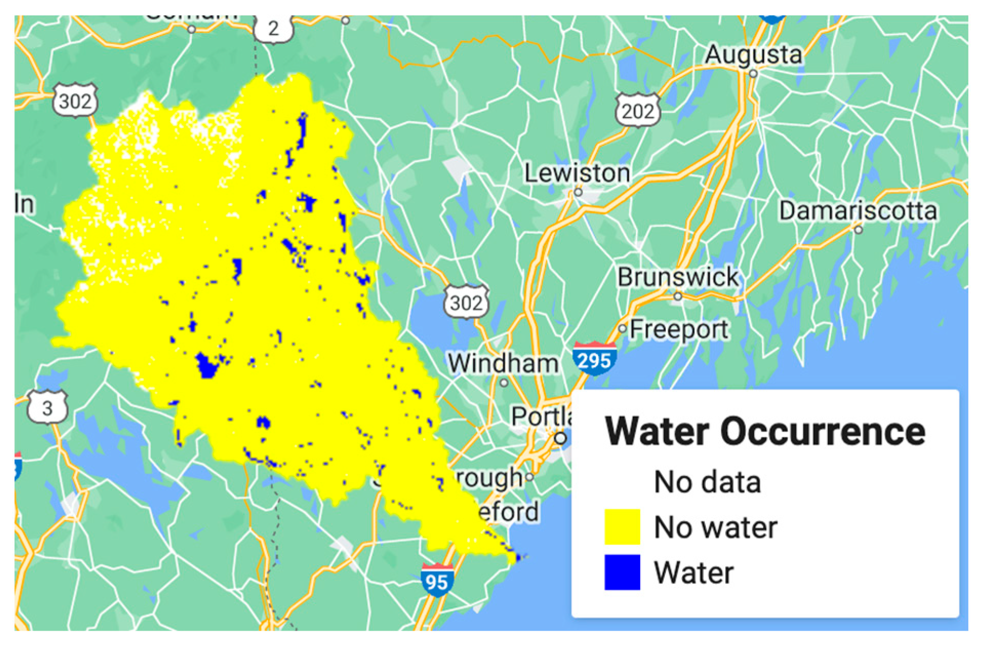
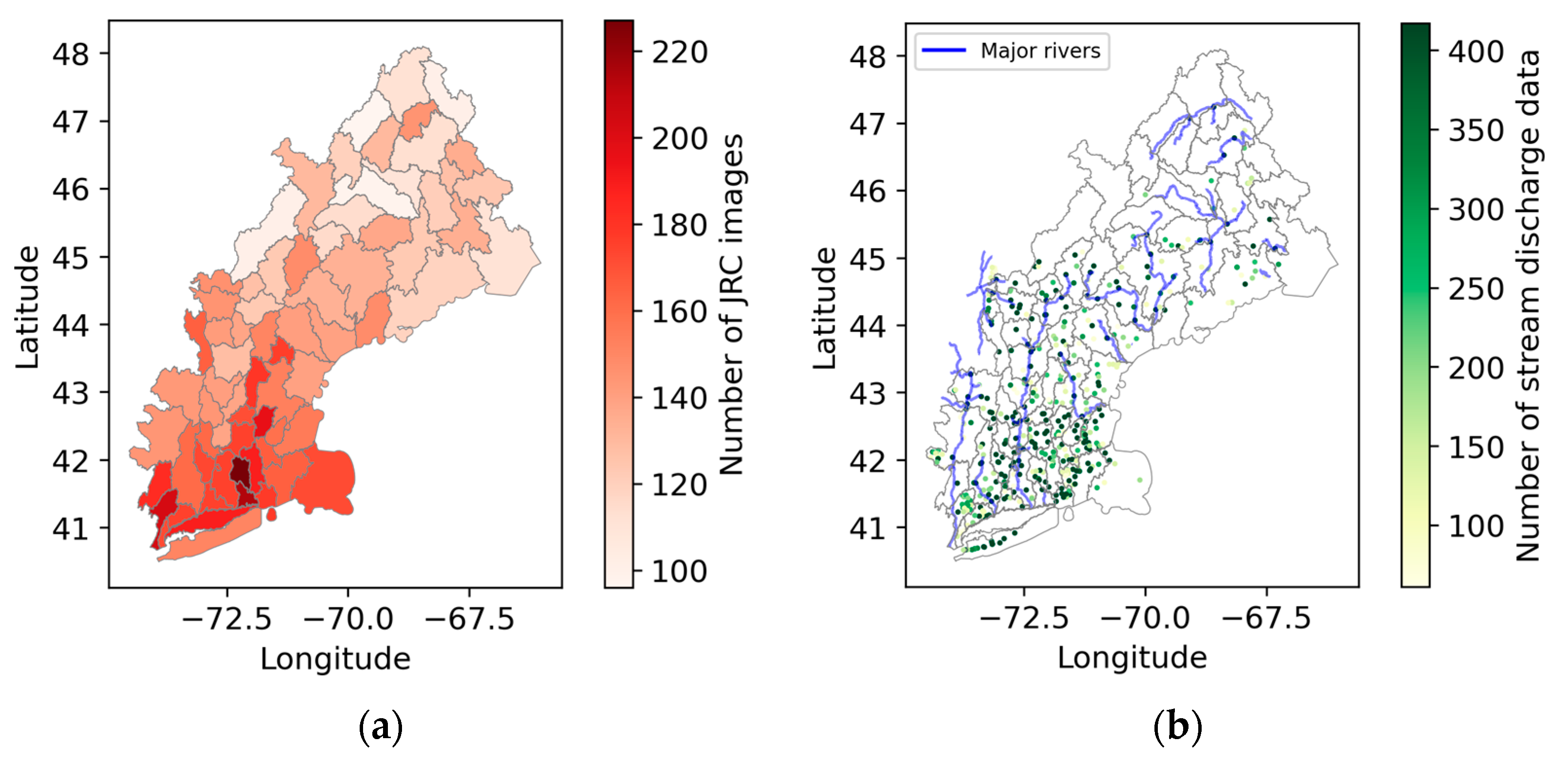
2.2. The Joint Research Centre Monthly Water History

The European Commission’s Joint Research Centre (JRC) provides long-term statistics of monthly maximum surface water extent (SWE) since April 1984. The JRC dataset is generated using satellite images from Landsat missions (Landsat 5, 7, and 8) with a spatial resolution of 30 m, and each pixel is classified as either water, non-water, or no data, combing all the satellite images in each month [13]. If a pixel is identified as water in any satellite images acquired during a given month, it is considered as water in the corresponding monthly dataset. All the water pixels are aggerated by month, representing the monthly maximum SWE. To derive the JRC monthly maximum SWE, we utilized the Google Earth Engine Editor platform [20]. The detailed process is illustrated in Appendix A.

In this study, we gathered monthly maximum SWE data from April 1984 to December 2018 (417 months) for each of the 70 HUCs in the New England region. In an ideal case of no missing SWE data, we would have 29,190 satellite images for all the HUCs. Only 10,290 satellite images, or 35%, were available. A screening process was conducted to eliminate images with missing data pixels exceeding 10%. This procedure aligns with the methodology discussed in [14], which employed a 5% threshold for the same purpose. Thus, for our study area, 10,258 images were used.

In Figure 1a, we depict the number of JRC images for each HUC throughout the whole collection period of 417 months. The count ranges from 96 to 227, with an average of 147 images. It is evident that the availability of JRC images exhibits significant variability across different HUCs, with a pronounced concentration of these images observed in the southern New England region.

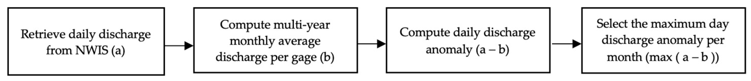
2.3. The US Geological Survey Daily Streamflow Discharge

Streamflow discharges are measured by the US Geological Survey (USGS) in real-time and averaged daily. Daily average streamflow data were accessed through the USGS National Water Information System (NWIS; https://waterdata.usgs.gov/nwis) using [21].

In total, 474 stream gages were collected for this study and an upward trend of the number of stream gages was observed during the study period. The number of stream discharge data varies by HUC, ranging from 61 to 417 with a mean of 276 months (see Figure 1b). The number of stream gages also varies by HUC, ranging from 1 to 32, with a mean of 8 stations. In certain HUCs, such as the northern New England region (eight HUCs) and Long Island Sound (one HUC), the absence of stream gage stations precluded their inclusion in the analysis, and, thus, these regions were excluded from the study. Furthermore, two consecutive days of streamflow discharge from one gage (gage 01103025) revealed negative discharge values. These anomalous values, deemed to be near zero and indicative of measurement errors or inconsistencies, were deleted for the sake of data integrity and accuracy.

As shown in Figure 2, a tradeoff between the number of gages and sample size is evident. As sample size increases, the number of gages with that specific sample size decreases. Out of the total 474 gages, only 175 have complete records spanning 417 months, while all 474 gages have at least 61 months of data. In the ridge regression in Section 3, we use only the 308 gages that have at least 200 months of data.

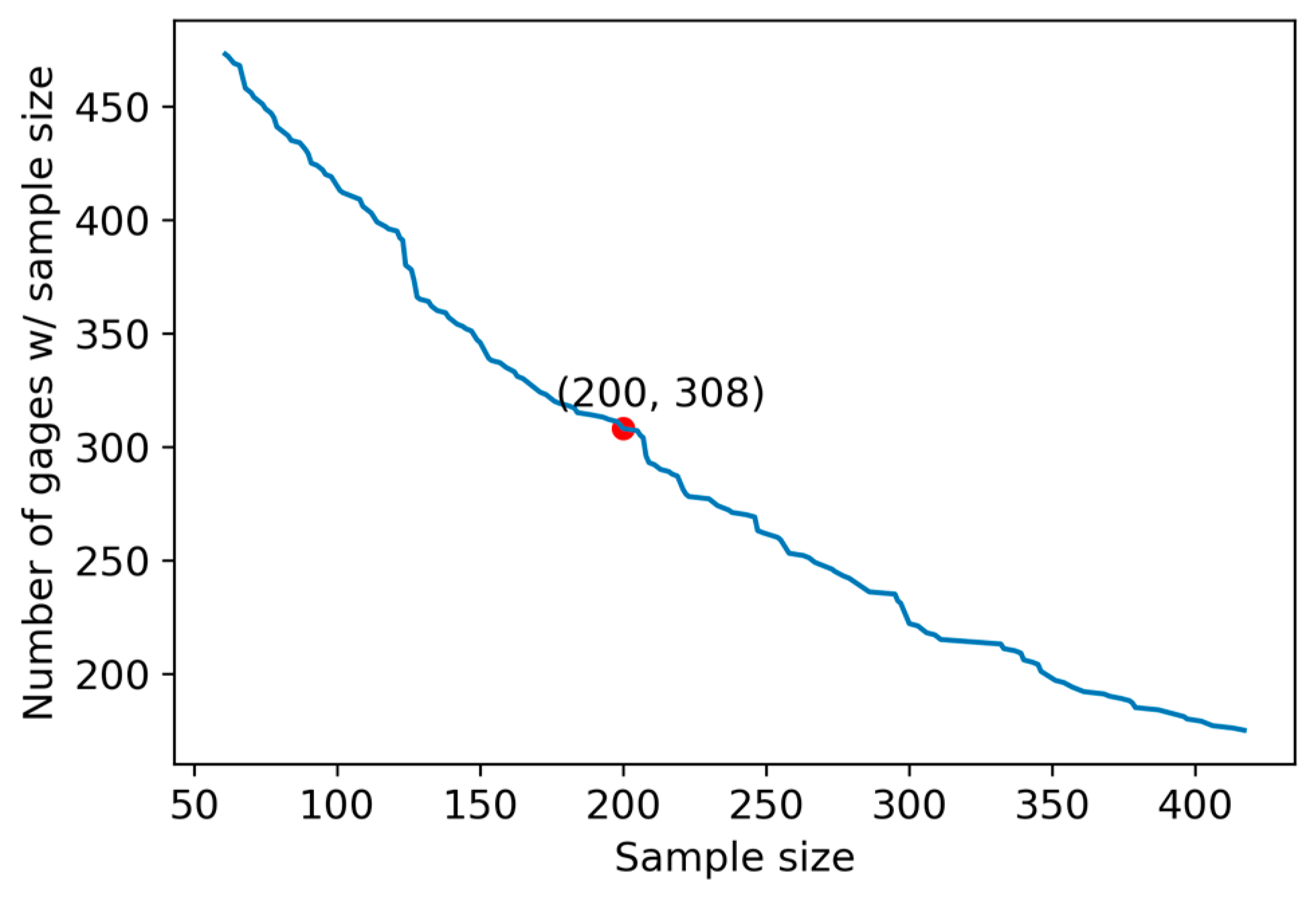
2.4. Pairing JRC Data with USGS Streamflow Discharge Data

To establish a complementary dataset for the JRC monthly maximum SWE, we employed a methodology based on the calculation of daily streamflow discharge anomaly. As shown in Figure 3, firstly, for each month, the daily streamflow discharge was obtained. If, on any given day, the daily streamflow discharge exceeded the corresponding multi-year monthly mean discharge, the daily streamflow discharge anomaly was obtained. The multi-year monthly mean discharge was computed from April 1984 to December 2018. Following this, we selected the maximum day streamflow discharge anomaly (SFDA) per month to pair it with the JRC monthly maximum SWE.

To ensure sufficient data for further analysis, we paired the JRC monthly maximum SWE with the USGS maximum day SFDA, retaining only the months where the paired dataset spans 30 months or more. In the following context, we use the paired SWE and SFDA to refer to the dataset.

In Figure 4, the time series plot shows SWE and SFDA within the same HUC 01060002. The SWE data exhibit a significant number of missing values. With the available data, the correlation between SWE and SFDA from each gage was denoted by the Spearman’s r (as seen in parentless).

3. Methods

3.1. Correlation Analysis

The present study employed a methodology similar to [14] but for a different domain, and instead of monthly averages of SFD we use SFDA to investigate the correlation with SWE. We opted to focus on HUCs that contained a minimum of three gages within their boundaries. This process guarantees a minimum number of gages to represent the spatial variations in a HUC at the expense of reducing their number.

To explore relationships between SWE and SFDA, we paired SWE and SFDA obtained from all gages in the study area individually. Spearman’s r was calculated between each paired SWE and SFDA, with the condition that the paired dataset contained a minimum of 30 data points. This criterion was applied to ensure that the correlation analysis was conducted with enough data for robust and meaningful results. In total, these two criterions reduced the number of HUCs for analysis, resulting in 45 HUCs meeting this selection criterion. Spearman’s r is a non-parametric measure of the monotonicity of the relationship between the paired datasets, which is expressed as:

$$r= \frac{cov(R\left(x\right), R\left(y\right))}{{\sigma }_{R\left(x\right)}{\sigma }_{R\left(y\right)}}$$

(1)

where $x$ and $y$ are the paired SFDA and SWE, $R\left(x\right)$ and $R\left(y\right)$ are rank transformed variables, $cov(R\left(x\right), R\left(y\right))$ is the covariance of the rank variables, and ${\sigma }_{R\left(x\right)}$ ${\sigma }_{R\left(y\right)}$ are the standard deviations of the rank variables. The Spearman’s r ranges from −1 to 1, where −1 indicates a strong negative correlation, 1 indicates a strong positive correlation, and 0 indicates no correlation.

3.2. Modeling SWE Using Ridge Regression

3.2.1. Data Transformation

SWE and SFDA were both transformed to ensure the variances were stabilized before the modeling. The Box–Cox transformation was used for transforming the remote sensing-derived hydrological variables [2]. The Box–Cox transformation is useful due to its various approaches, for instance, square roots, logarithms, and squares [22]. In this study, we applied the square roots for the SWE. Since SFDA contains non-positive values, the logarithm transformation was applied after a shift to ensure all the values were positive.

3.2.2. Model Selection

Stream gages displaying these high correlations with SWE can serve as valuable candidates for modeling SWE. The screening of such stream gages for SWE modeling involves the application of ridge regression, a regularization technique within linear regression. Ridge regression plays a pivotal role in enhancing model performance by addressing challenges related to multicollinearity in the dataset and facilitating variable selection [23,24]. It achieves this by constraining coefficients using a regularization term, thereby helping to identify significant predictors while keeping others close to zero. The mathematical equation of the ordinary (unconstrained) linear regression is expressed as:

$$\beta X=y$$

(2)

where $X$ is the matrix ($n\times p$) of transformed SFDA, n is the number of observations, p is the number of stream gages, $\beta$ = ${\left[{\beta }_1 {\beta }_2\dots {\beta }_p\right]}^T$ is a vector of weights, $y={\left[y_1 y_2\dots y_n\right]}^T$ is a vector of transformed SWE, and T denotes the transpose.

The cost function of the above linear regression,$J\left(\beta \right),$ is the sum of squares of errors (SSE):

$$J\left(\beta \right)=MSE\left(\beta \right)={\left(\beta X-y\right)}^T\left(\beta X-y\right)$$

(3)

For ridge regression, a regularization term is added; thereby, the cost function, $J_r\left(\beta \right)$, of a ridge regression, is expressed as:

$${J_r\left(\beta \right)=\left(\beta X-y\right)}^T\left(\beta X-y\right)+\lambda {\beta }^T\beta$$

(4)

where $\lambda$ is a regularization parameter that controls the regularization strength.

The solution to the ridge regression, as proposed by [25], is as follows:

$$\beta \left(\lambda \right)={\left(X^{T}X+\lambda \mathit{I}\right)}^{-1}{X}^{T}y$$

(5)

where $\beta \left(\lambda \right)$ are weights of the ridge regression, and I is the identity matrix.

3.2.3. Model Set-Up, Training, and Evaluation

For each HUC, SWE was paired with SFDA from all gages in the study area and the missing values in each gage were imputed using their medians. To ensure the robustness of our analysis, we exclusively considered gages with a data record spanning more than 200 months for pairing with each respective HUC, reducing the gages to 308. This objective aims to maintain the dataset’s integrity and serves to mitigate the influence of noise arising from the imputation of missing values, which was performed using the median. Then, the SFDA was standardized; thereby, the values are centered around the zero mean with one standard deviation. In our analysis, we employed ridge regression for each of the 45 HUCs. To facilitate this process, we divided each dataset into two subsets: a training set comprising 80% of the data and a test set containing the remaining 20%.

To determine the optimal value of the regularization parameter (λ), we employed a fivefold cross-validation procedure. This involved evaluating λ over a range from 1 to 100. Once the optimal λ was identified through cross-validation, it was subsequently utilized in the ridge regression model to train the data, ensuring the most effective regularization for each HUC.

The model was evaluated on the test set using root-mean-square error (RMSE), normalized RMSE (NRMSE) and R squared (R²). They are expressed as:

$$RMSE={\left(\frac{{\left(\beta X-y\right)}^T\left(\beta X-y\right)}{n}\right)}^{1/2}$$

(6)

$$NRMSE=\frac{RMSE}{\overline{y}}$$

(7)

$$R^2=1-\frac{{\left(\beta X-y\right)}^T(\beta X-y)}{{\left(y-\overline{y}\right)}^T(y-\overline{y})}$$

(8)

where $\overline{y}$ is the average observed SWE.

The Nash–Sutcliffe efficiency index (E_f), as proposed by Nash and Sutcliffe, is another metric for assessing the goodness-of-fit for models (1971). E_f can be applied to different model types without the constraints of the assumptions of linear models. For linear and unbiased models, E_f aligns with the R² since E_f is sensitive to the bias and E_f equals to zero if the relative bias reaches 40% [26].

4. Results

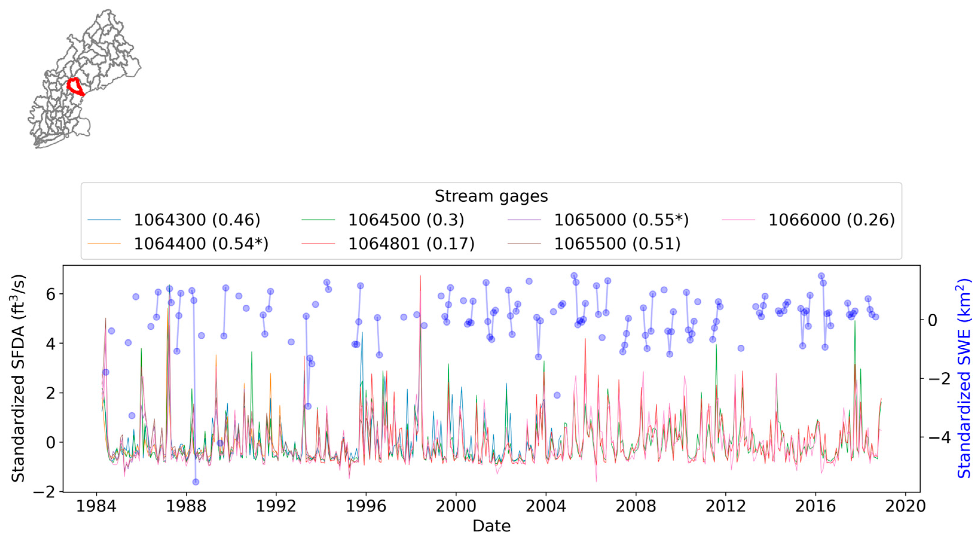
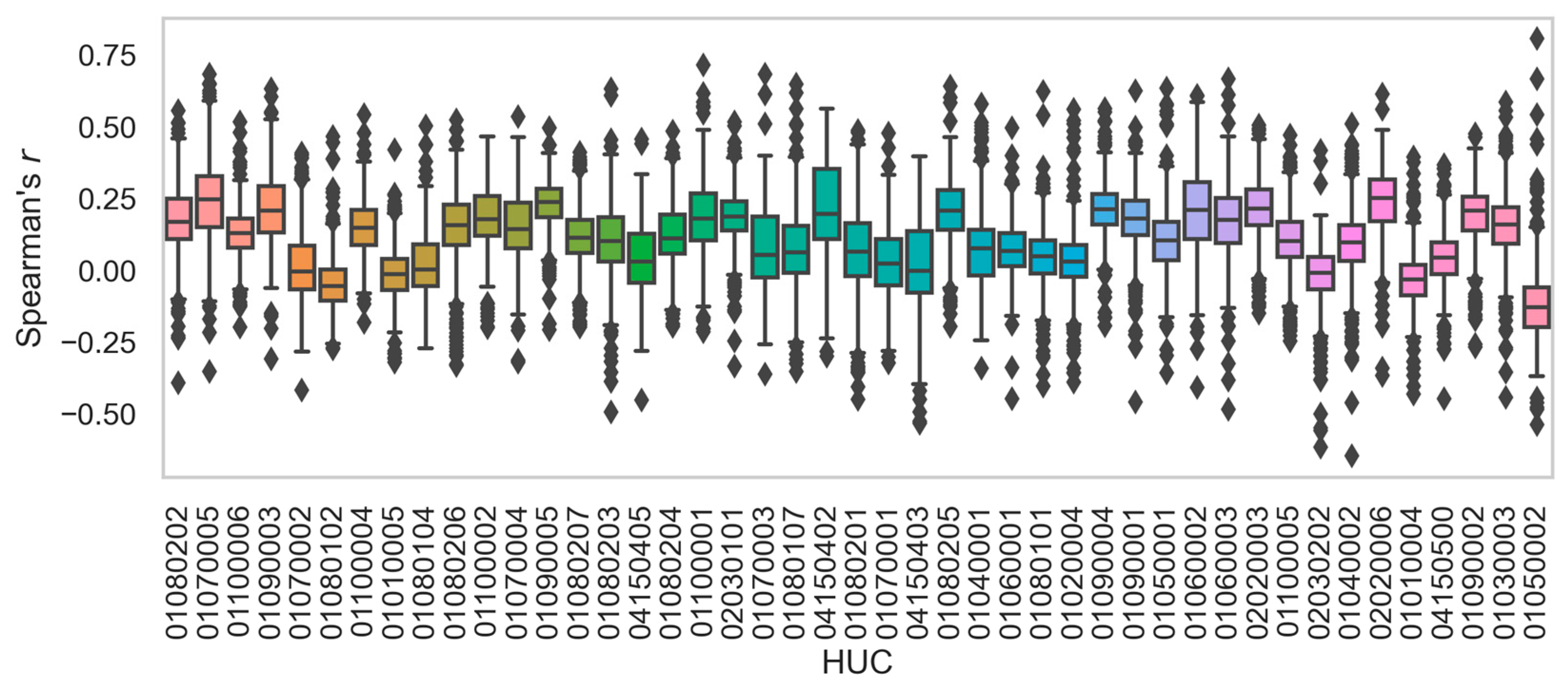
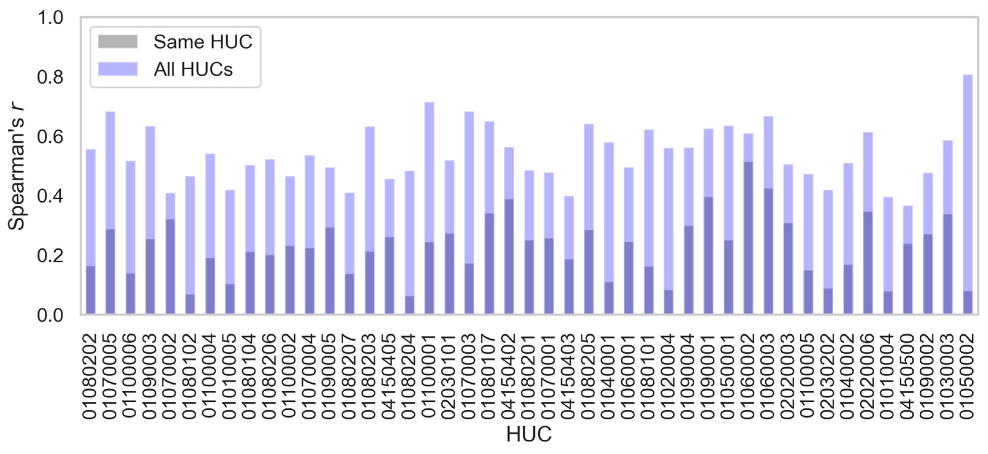
4.1. Correlations between SWE and SFDA

Figure 5 illustrates the variation in Spearman’s r across different HUCs, displaying a broad range of values spanning from negative to positive. Some HUCs exhibit strong positive correlations exceeding 0.7. Upon arranging the HUCs in ascending order based on the size of their respective basins, there appears to be no discernible correlation between the magnitude of the correlation coefficient and the size of the basins.

In Figure 6, we present the maximum correlation achieved in each HUC under two distinct conditions: SWE and SFDA of gages located inside of each HUC and the same correlation but considering all gages in the study area. The results illustrate notable differences between the two scenarios, suggesting that the hydrological boundary plays a crucial role in influencing the correlation strength. As depicted in Figure 6, most of the correlations are weak for SWE and SFDA in the same HUC, which is consistent with findings from previous studies [14,27]. Furthermore, the correlations within the same HUC tend to exhibit lower values compared to those observed outside of the reference HUC. This finding suggests that when the hydrological boundary is not a restrictive factor, the correlations between SWE and SFDA tend to be higher.

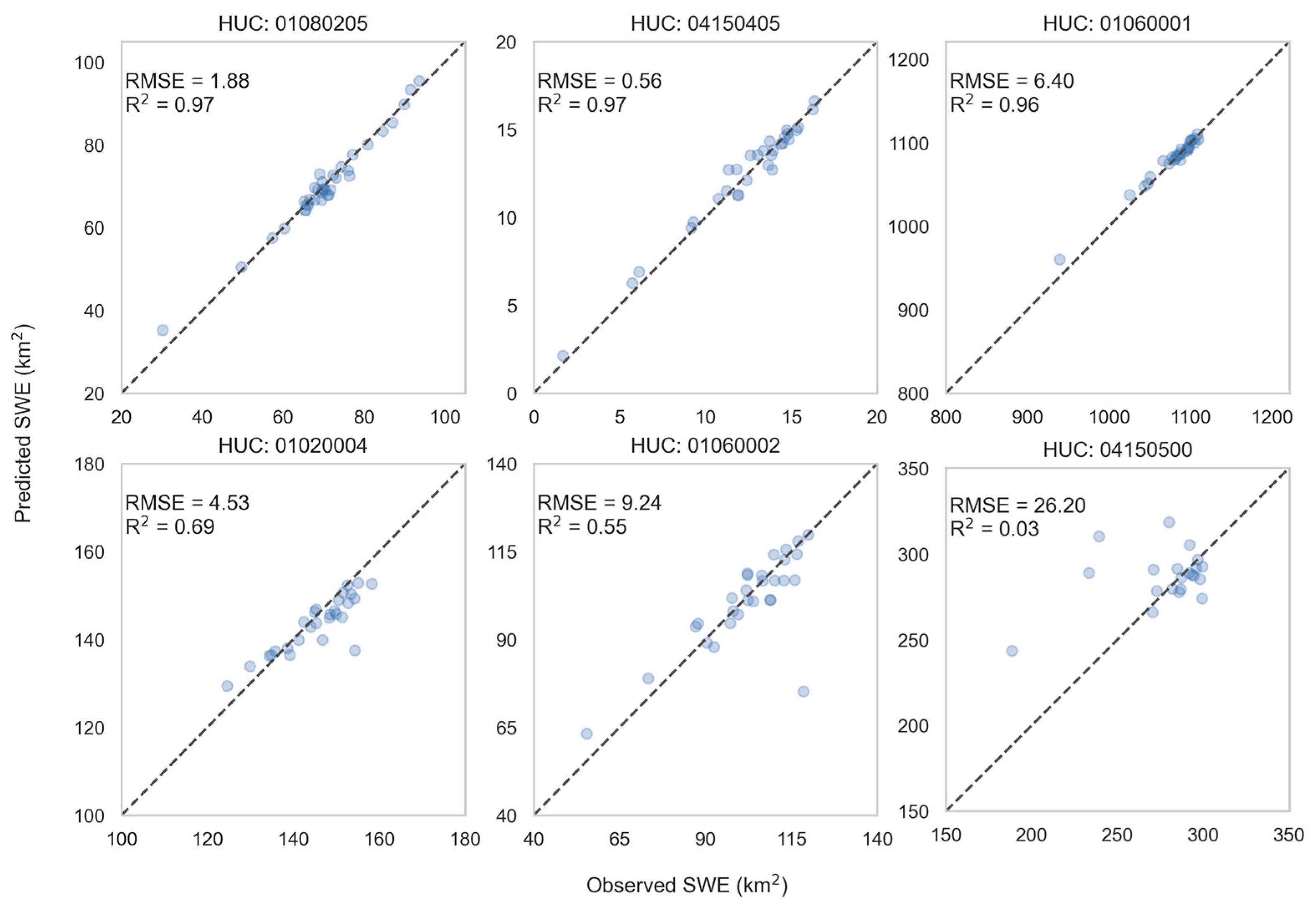
4.2. Ridge Regression Model Performance

Ridge regression was constructed for each HUC using SFDA of all the gages (308 in total) in the study area.

The training sample size ranges from 80 to 181 by HUC. Figure 7 presents performance metrics obtained from each ridge regression model, which are RMSE, NRMSE, and R². The RMSE values exhibit a broad range, with larger values in the coastal HUCs. Most of the HUCs have an RMSE below 10. NRMSE shows a good fit, with 44 out of 45 HUCs achieving values below 0.1. The R² scores reveal that 42 out of 45 models achieve R² scores greater than 0.7. The E_f results are consistent with the R² values due to the marginal relative bias, ranging from −0.02 to 0.3. Overall, ridge regression models showed promising results across most HUCs, though performance varied by HUCs.

In Figure 8, we showed the scatter plots of six models as an example to show their goodness of fit on the test data. The first row consists of three models with the highest R² scores, where most of the points align closely with the diagonal line (1:1 line), demonstrating a high degree of consistency between predicted and observed SWE. In contrast, the second row shows three models with the lowest R² scores. While some data points still appear clustered around the diagonal line, the presence of outliers significantly affects the overall model fit.

4.3. Interpolated Time Series of SWE

In HUC 01010005, the trained ridge regression model was used to interpolate the missing values in SWE to create the full time series. As shown in Figure 9, the predicted and observed SWE distributions are closely aligned with a noticeable shift. Additionally, the predicted SWE distribution is more concentrated around 6.5 km², while the observed SWE distribution centers around 8 km². This shift was also seen in most HUCs. To address this discrepancy, one potential solution involves introducing a constraint that penalizes deviations in the weights from the observed mean [28,29].

Figure 10a is an example of using the above-mentioned model to interpolate the time series of SWE from 2010 to 2018. The model filled the gaps in the observed SWE with predicted values and completed the time series. It is noted that the model demonstrated its capability to successfully interpolate even in cases of substantial data gaps. Furthermore, the model captured the dynamic nature of SFDA, encompassing fluctuations rather than being limited to monotonic trends. It is evident that the model tends to predict lower values, displaying a noticeable skew towards the lower end of the distribution.

As seen in Figure 10b, the weights are distributed across the study domain, with most gages displaying low weights (depicted as yellow dots), while only one gage outside of the reference HUC exhibits high weights (depicted as green dots). Several factors could impact the gage’s importance, including complex hydrological interactions, intricate flow paths, and various environmental factors despite their geographical distance from the analyzed HUC. Additionally, data quality, including the reliability and accuracy of measurements, might elevate the gage’s importance in the model. Furthermore, model configuration, regularization strength, and outliers can also play a role in determining the weights of the gages.

5. Discussion

5.1. Data Limitations and Challenges

The analysis above is subject to various data limitations and challenges that can significantly impact the selection and performance of different modeling methods. In this study, we encountered several key data limitations in both JRC monthly maximum SWE and the streamflow discharge data.

The JRC monthly maximum SWE serves as a critical data source for understanding the temporal distribution and the statistics of water surfaces. However, its reliability is inherently influenced by satellite imagery availability which, in turn, depends on weather conditions. Cloud cover and atmospheric conditions can hinder the acquisition of satellite images, leading to gaps or missing data in the JRC water history dataset. When significant portions of the data are missing, the ability to produce meaningful temporal patterns is compromised, affecting the overall performance of the model.

Streamflow discharge data is a fundamental component in statistical modeling, as it directly reflects the water flow in the rivers and streams. However, obtaining accurate and reliable streamflow data can be challenging for various reasons. One significant challenge arises from the manual intervention of streamflow discharge data. Human error in data entry could introduce inaccuracies and inconsistencies, leading to potential outliers or noise in the dataset. Such inconsistencies might affect the quality of results and the reliability of the models.

5.2. Alternative Methods for Exploring the SWE-SFDA Relationship

Alternative methods, including lasso regression, were also explored in this study. Lasso regression is a regularization technique that shares similarities with ridge regression; the primary advantage of lasso regression is its ability to perform feature selection by shrinking less important coefficients to exactly zero [30]. As a result, lasso can effectively eliminate irrelevant variables from the model, leading to a sparse model with a reduced number of features. Despite its usefulness in feature selection, lasso regression may not be the most suitable approach for estimating surface water extent in certain scenarios. This is because, in some cases, setting coefficients to exactly zero led to unrealistic SWE estimates.

5.3. Additional Factors in the SWE-SFDA Relationship

In this study, we primarily focused on streamflow discharge anomaly as a feature for estimating surface water extent. The advantage of this is that there is a long record of data collected since 1984 at high temporal resolution. Moreover, with the long record, it is possible to consider, for instance, relationships that are conditional to seasons. However, it is important to acknowledge that additional factors, such as river characteristics (e.g., river width, slope, and depth), hydro-meteorological conditions, and annual/seasonal variations can significantly impact the relationship between streamflow discharge anomaly and surface water extent. Incorporating these additional features can enhance the performance of the model by capturing the complexity of hydrological processes influenced by the river’s physical characteristics. Moreover, the influence of climate change further compounds the impact on the seasonal patterns, thereby affecting the overall seasonality of streamflow discharge [31]. It is crucial to recognize that the non-stationarity of hydro-meteorological variables, induced by climate change, has significant implications for both annual and seasonal patterns [32,33,34].

By combining all these factors into the modeling process, we can gain a more comprehensive understanding of the hydrological system, leading to improved relationships and a deeper insight into the hydrological patterns within each HUC. Future research efforts could explore the integration of these factors and consider seasonal variations to refine the models and better represent real-world conditions.

6. Conclusions

In this paper, we conducted a comprehensive investigation to explore the relationship between surface water extent and streamflow discharge anomaly. Through the implementation of ridge regression, we established a robust relationship between streamflow discharge anomaly and surface water extent for most of the HUCs in the New England region.

Two distinctive aspects of our approach are introduced. Firstly, we derived streamflow discharge anomaly to match JRC surface water extent. By aligning and combining these datasets, we obtained a more refined representation of hydrological behavior within each HUC. This anomaly-based approach allowed us to focus on hydrological deviations and anomalies, providing a deeper insight into the variations and dynamics of streamflow discharge across the study domain. Secondly, we used a ridge regression model with streamflow discharge anomaly from selected gages for each HUC. This allowed us to capture the interconnected nature of hydrological processes, providing an understanding of how streamflow discharge anomaly varies across different regions. Ridge regression effectively identified the gage stations that contribute to the most to the relationship with each HUC. It assigned significant weights to the important predictors, a robust method for feature selection.

Additionally, our study addressed the impact of data limitations and the potential influence of additional factors, such as river characteristics, on the relationship between surface water extent and streamflow discharge anomaly. While exploring alternative modeling techniques, including lasso regression, we found that ridge regression remained more effective for our dataset.

In conclusion, our study provides insights into the relationship between surface water extent and streamflow discharge anomaly. These distinctive aspects, combined with the robust ridge regression approach, provide an understanding of hydrological behavior. Furthermore, gap-filled Landsat-derived surface water extent time series establish essential baselines for water resource management, inundation mapping, and land-use decisions.

Future research efforts will be focused on (1) exploring the integration of diverse datasets and considering additional factors to further enhance the correlation between surface water extent and streamflow discharge anomaly and (2) improving the screening of the stream gages that carry more weight in determining surface water extent estimates and investigating geospatial correlations or patterns. The potential applications of this research extend to surface water extent mapping, especially during times when satellite imagery is unavailable. Advancements in data collection and analysis techniques will enable more accurate and insightful estimates, supporting better water resource management and decision-making.

References

1. Smith, L.C. Satellite Remote Sensing of River Inundation Area, Stage, and Discharge: A Review. Hydrol. Process. 1997, 11, 1427–1439. [Google Scholar] [CrossRef]
2. Loaiza, J.G.; Rangel-Peraza, J.G.; Monjardín-Armenta, S.A.; Bustos-Terrones, Y.A.; Bandala, E.R.; Sanhouse-García, A.J.; Rentería-Guevara, S.A. Surface Water Quality Assessment through Remote Sensing Based on the Box–Cox Transformation and Linear Regression. Water 2023, 15, 2606. [Google Scholar] [CrossRef]
3. Zhang, F.; Shao, Y.; Huang, H.; Bahtebay, J. Review of Urban Remote Sensing Research in the Last Two Decades. Acta Ecol. Sin. 2021, 41, 3255–3276. [Google Scholar]
4. Wang, Y.; Colby, J.D.; Mulcahy, K.A. An Efficient Method for Mapping Flood Extent in a Coastal Floodplain Using Landsat TM and DEM Data. Int. J. Remote Sens. 2002, 23, 3681–3696. [Google Scholar] [CrossRef]
5. Qi, S.; Brown, D.G.; Tian, Q.; Jiang, L.; Zhao, T.; Bergen, K.M. Inundation Extent and Flood Frequency Mapping Using LANDSAT Imagery and Digital Elevation Models. GIScience Remote Sens. 2009, 46, 101–127. [Google Scholar] [CrossRef]
6. Grimaldi, S.; Li, Y.; Pauwels, V.R.; Walker, J.P. Remote Sensing-Derived Water Extent and Level to Constrain Hydraulic Flood Forecasting Models: Opportunities and Challenges. Surv. Geophys. 2016, 37, 977–1034. [Google Scholar] [CrossRef]
7. Shen, X.; Wang, D.; Mao, K.; Anagnostou, E.; Hong, Y. Inundation Extent Mapping by Synthetic Aperture Radar: A Review. Remote Sens. 2019, 11, 879. [Google Scholar] [CrossRef]
8. Shen, X.; Anagnostou, E.N.; Allen, G.H.; Robert Brakenridge, G.; Kettner, A.J. Near-Real-Time Non-Obstructed Flood Inundation Mapping Using Synthetic Aperture Radar. Remote Sens. Environ. 2019, 221, 302–315. [Google Scholar] [CrossRef]
9. Yang, Q.; Shen, X.; Anagnostou, E.N.; Mo, C.; Eggleston, J.R.; Kettner, A.J. A High-Resolution Flood Inundation Archive (2016–the Present) from Sentinel-1 SAR Imagery over CONUS. Bull. Am. Meteorol. Soc. 2021, 102, E1064–E1079. [Google Scholar] [CrossRef]
10. Short, N.M. The Landsat Tutorial Workbook: Basics of Satellite Remote Sensing; National Aeronautics and Space Administration, Scientific and Technical Information Branch: Washington, DC, USA, 1982. [Google Scholar]
11. Jutz, S.; Milagro-Pérez, M.P. Copernicus: The European Earth Observation Programme. Rev. Teledetec. 2020, 56, 5–11. [Google Scholar] [CrossRef]
12. Vuolo, F.; Ng, W.-T.; Atzberger, C. Smoothing and Gap-Filling of High Resolution Multi-Spectral Time Series: Example of Landsat Data. Int. J. Appl. Earth Obs. Geoinf. 2017, 57, 202–213. [Google Scholar] [CrossRef]
13. Pekel, J.-F.; Cottam, A.; Gorelick, N.; Belward, A.S. High-Resolution Mapping of Global Surface Water and Its Long-Term Changes. Nature 2016, 540, 418–422. [Google Scholar] [CrossRef]
14. Walker, J.J.; Soulard, C.E.; Petrakis, R.E. Integrating Stream Gage Data and Landsat Imagery to Complete Time-Series of Surface Water Extents in Central Valley, California. Int. J. Appl. Earth Obs. Geoinf. 2020, 84, 101973. [Google Scholar] [CrossRef]
15. Usachev, V.F. Evaluation of Flood Plain Inundations by Remote Sensing Methods. Hydrol. Appl. Remote Sens. Remote Data Transm. 1983, 145, 475–482. [Google Scholar]
16. Gleason, C.J.; Smith, L.C. Toward Global Mapping of River Discharge Using Satellite Images and At-Many-Stations Hydraulic Geometry. Proc. Natl. Acad. Sci. USA 2014, 111, 4788–4791. [Google Scholar] [CrossRef] [PubMed]
17. Robert Brakenridge, G.; Cohen, S.; Kettner, A.J.; De Groeve, T.; Nghiem, S.V.; Syvitski, J.P.M.; Fekete, B.M. Calibration of Satellite Measurements of River Discharge Using a Global Hydrology Model. J. Hydrol. 2012, 475, 123–136. [Google Scholar] [CrossRef]
18. Anh, D.T.L.; Aires, F. River Discharge Estimation Based on Satellite Water Extent and Topography: An Application over the Amazon. J. Hydrometeorol. 2019, 20, 1851–1866. [Google Scholar] [CrossRef]
19. Alsdorf, D.E.; Rodríguez, E.; Lettenmaier, D.P. Measuring Surface Water from Space. Rev. Geophys. 2007, 45, RG2002. [Google Scholar] [CrossRef]
20. Gorelick, N.; Hancher, M.; Dixon, M.; Ilyushchenko, S.; Thau, D.; Moore, R. Google Earth Engine: Planetary-Scale Geospatial Analysis for Everyone. Remote Sens. Environ. 2017, 202, 18–27. [Google Scholar] [CrossRef]
21. Hodson, T.O.; Hariharan, J.A.; Black, S.; Horsburgh, J.S. Dataretrieval 0.1 (Python): A Python Package for Discovering and Retrieving Water Data Available from U.S. Federal Hydrologic Web Services; U.S. Geological Survey Software Release; U.S. Geological Survey: Reston, VA, USA, 2023.
22. Vélez, J.I.; Correa, J.C.; Marmolejo-Ramos, F. A New Approach to the Box–Cox Transformation. Front. Appl. Math. Stat. 2015, 1, 12. [Google Scholar] [CrossRef]
23. Marquardt, D.W.; Snee, R.D. Ridge Regression in Practice. Am. Stat. 1975, 29, 3–20. [Google Scholar] [CrossRef]
24. Tikhonov, A.N. Solution of Incorrectly Formulated Problems and the Regularization Method. Sov. Math. Dokl. 1963, 4, 1035–1038. [Google Scholar]
25. Hoerl, A.E.; Kennard, R.W. Ridge Regression: Biased Estimation for Nonorthogonal Problems. Technometrics 1970, 12, 55–67. [Google Scholar] [CrossRef]
26. McCuen, R.; Knight, Z.; Cutter, A. Evaluation of the Nash–Sutcliffe Efficiency Index. J. Hydrol. Eng. 2006, 11, 597–602. [Google Scholar] [CrossRef]
27. Van Dijk, A.I.J.M.; Brakenridge, G.R.; Kettner, A.J.; Beck, H.E.; De Groeve, T.; Schellekens, J. River Gauging at Global Scale Using Optical and Passive Microwave Remote Sensing. Water Resour. Res. 2016, 52, 6404–6418. [Google Scholar] [CrossRef]
28. Delsole, T. A Bayesian Framework for Multimodel Regression. J. Clim. 2007, 20, 2810–2826. [Google Scholar] [CrossRef]
29. Peña, M.; Dool, H. van den Consolidation of Multimodel Forecasts by Ridge Regression: Application to Pacific Sea Surface Temperature. J. Clim. 2008, 21, 6521–6538. [Google Scholar] [CrossRef]
30. Ranstam, J.; Cook, J.A. LASSO Regression. Br. J. Surg. 2018, 105, 1348. [Google Scholar] [CrossRef]
31. van Vliet, M.T.H.; Franssen, W.H.P.; Yearsley, J.R.; Ludwig, F.; Haddeland, I.; Lettenmaier, D.P.; Kabat, P. Global River Discharge and Water Temperature under Climate Change. Glob. Environ. Chang. 2013, 23, 450–464. [Google Scholar] [CrossRef]
32. Kousali, M.; Salarijazi, M.; Ghorbani, K. Estimation of Non-Stationary Behavior in Annual and Seasonal Surface Freshwater Volume Discharged into the Gorgan Bay, Iran. Nat. Resour. Res. 2022, 31, 835–847. [Google Scholar] [CrossRef]
33. Modabber-Azizi, S.; Salarijazi, M.; Ghorbani, K. A Novel Approach to Recognize the Long-Term Spatial-Temporal Pattern of Dry and Wet Years over Iran. Phys. Chem. Earth Parts ABC 2023, 131, 103426. [Google Scholar] [CrossRef]
34. Salarijazi, M.; Ghorbani, K.; Mohammadi, M.; Ahmadianfar, I.; Mohammadrezapour, O.; Naser, M.H.; Yaseen, Z.M. Spatial-Temporal Estimation of Maximum Temperature High Returns Periods for Annual Time Series Considering Stationary/Nonstationary Approaches in Iran Urban Area. Urban Clim. 2023, 49, 101504. [Google Scholar] [CrossRef]
Figure 1. (a) Number of JRC images per HUC. The 10% rule of screening process is applied. (b) Number of stream discharge data per gage.
Water 16 00250 g001
Figure 2. The number of gages relative to sample size. Sample size is the number of months of stream discharge data. The red dot depicts 308 gages with at least 200 months of data.
Water 16 00250 g002
Figure 3. Flowchart of the process to obtain the maximum day streamflow discharge anomality (SFDA) per month.
Water 16 00250 g003
Figure 4. Time series and correlations between SWE and SFDA in HUC 01060002 (location shown in the left corner with the red contour). Spearman’s r is calculated and shown next to the gages in the legend; values are marked as * when the sample size is less than 30.
Water 16 00250 g004
Figure 5. Spearman’s r between paired SWE and SFDA of gages in the study area. Data are arranged in ascending order of basin size, from small to large (from left to right).
Water 16 00250 g005
Figure 6. Gray bars show the maximum correlation between SWE and SFDA of gages within the same HUC; purple bars show the same correlation but considering all gages in the study area. Data is arranged in ascending order of basin size, from small to large (from left to right).
Water 16 00250 g006
Figure 7. Ridge regression model performance for 45 HUCs in terms of RMSE, NRMSE, and R2. HUCs shown in white have been excluded from the analysis (refer to Section 3.1 for more details).
Water 16 00250 g007
Figure 8. Examples of 6 ridge regression models with their goodness of fit on the test set. The first row consists of 3 models with the highest R2 scores, while the second row consists of 3 models with the lowest R2 scores. Diagonal line is the 1:1 line.
Water 16 00250 g008
Figure 9. Histogram and distribution of the observed and predicted SWE in HUC 01010005.
Water 16 00250 g009
Figure 10. (a) Observed, predicted, and full (interpolated) SWE time series for HUC 01010005 from 2010 to 2018. (b) Weights of ridge regression for HUC 01010005. HUC 01010005 is shown with the red contour.
Water 16 00250 g010
Disclaimer/Publisher’s Note: The statements, opinions and data contained in all publications are solely those of the individual author(s) and contributor(s) and not of MDPI and/or the editor(s). MDPI and/or the editor(s) disclaim responsibility for any injury to people or property resulting from any ideas, methods, instructions or products referred to in the content.