Evolution Trend of Depth to Groundwater and Agricultural Water-Saving Measure Threshold under Its Constraints: A Case Study in Helan Irrigated Areas, Northwest China

Abstract

Water conservation is imperative for alleviating water shortages and fostering the establishment of a water-saving society. However, the implementation of water-saving measures caused an increase in the depth to groundwater, resulting in ecological issues. Therefore, reasonable water saving should consider the appropriate depth to groundwater and its evolution trend. This study focuses on the Helan irrigation area in Ningxia as the research subject, aiming to establish thresholds for agricultural water-saving measures while considering constraints by depth to groundwater. The evolution trend of depth to groundwater from 1995 to 2018 was analyzed using the k-Shape cluster and complete ensemble empirical mode decomposition with adaptive noise (CEEMDAN) methods. Then, the thresholds of agricultural water-saving measures involved comparing groundwater numerical simulation results for water-saving scenarios, with the control area of ecological groundwater table depth and water shortage rate serving as the evaluation indices. The thresholds for implementing agricultural water-saving measures are as follows: the canal water utilization coefficient is set at 0.62; the proportion of water-efficient irrigation areas to effective irrigation areas should be 40% in the Yellow River irrigation area and 90% in the pumps-up Yellow River irrigation area; additionally, a reduction of 75% in the rice planting area is targeted.

1. Introduction

Water scarcity poses a significant challenge to sustainable economic and social development worldwide, particularly in arid and semi-arid regions [1,2,3]. Due to the scarcity of water resources, conflicts in water usage have intensified between production and ecology, agriculture and other industries, as well as upstream and downstream regions within river basins, even extending to various administrative boundaries [4]. Agricultural irrigation, being the largest consumer of water resources, accounts for approximately 70% of global freshwater usage and even surpasses 90% in certain arid regions [5]. In the semi-arid region of northwest China, the irrigation sector constitutes over 80% of the overall water usage [6,7]. Therefore, the implementation of the agricultural water conservation project in irrigated areas is an important way to improve water use efficiency and effectively reduce the conflict between supply and demand for regional water resources. It also plays a very important strategic role in ensuring water security, food security, ecological security, and sustainable agricultural development. In 2000, China put forward the proposal of establishing a water-saving society.

In addition to the aforementioned benefits, it is imperative to acknowledge that the implementation of water-saving measures can also yield adverse effects. The primary sources of groundwater recharge are surface water seepage and precipitation infiltration, while most water-saving measures tend to diminish the recharge of groundwater. The irrigation area in northwest China, characterized by limited precipitation, relies heavily on canal system seepage and field irrigation water infiltration for groundwater recharge [8,9]. Agricultural water-saving measures primarily encompass the implementation of canal lining, adoption of water-efficient irrigation technology, land leveling practices, and adjustment of planting structure. The application of canal lining and water-efficient irrigation technology directly reduces groundwater recharge, thereby altering the regional hydrological cycle and increasing the depth to groundwater (DTG) [10,11]. In irrigated areas, an increase in DTG will lead to a reduction in soil water storage [12] and the degradation of groundwater quality [13], thereby impacting the normal growth of crops and compromising the quantity and quality of agricultural drainage [5]. Consequently, numerous scholars have extensively investigated the impact of water-saving measures on spatiotemporal variations in groundwater levels and associated influencing factors [3,14,15,16]. However, the current research landscape lacks sufficient attention to investigate the appropriate level of water-saving intensity comprehensively. The appropriate water-saving intensity in this study primarily refers to the upper threshold of implementing routine agricultural water-saving measures in irrigated areas.

Scenario analysis is a prevalent approach in the investigation of water-saving strategies [7,14,15,17,18]. However, most existing water-saving scenario schemes primarily focus on surface and underground water supply planning within the study area, overlooking the dynamic changes in DTG trends following years of implementing water-saving measures. In regions where the DTG exhibits an increasing trend, it is unsuitable to adopt identical water-saving measures or implement equivalent water-saving intensity as in areas where the DTG remains stable or decreases. In this study, the DTG trend in the study area since the initiation of water-saving transformation in 1995 was comprehensively incorporated into the setting of water-saving scenario schemes. The DTG change is a complex and dynamic process that exhibits nonlinearity and non-stationarity. Therefore, to gain a more comprehensive understanding of the implications of water conservation project implementation on the DTG dynamics, it is crucial to employ sophisticated statistical techniques to meticulously delineate its dynamic patterns. Currently, sophisticated statistical approaches employed in the analysis of DTG dynamics include wavelet transform (WT), empirical mode decomposition (EMD), ensemble empirical mode decomposition (EEMD), and complementary ensemble empirical mode decomposition (CEEMD) [19,20,21,22,23,24,25,26,27,28]. Complete ensemble empirical mode decomposition with adaptive noise (CEEMDAN) proposed by Torres et al. [29], which adds specific white noise to each scale residual component of the decomposition and obtains the intrinsic mode function (IMF) by calculating the unique residual, can efficiently separate the periodic factors influencing signal trends from the inherent trend of the signal. Due to the integrated influence of natural conditions and anthropogenic activities, as well as the cyclical variations exhibited by the majority of naturally occurring influencing factors, the CEEMDAN method is more suitable for analyzing the evolution trend of DTG influenced by human factors such as water saving. Furthermore, the regional specificity of DTG evolutionary traits exhibits unique characteristics. Therefore, clustering analysis is frequently employed as a data preprocessing technique to enhance the comprehension of aquifer dynamics [30,31,32,33,34,35,36,37]. The majority of clustering methods employed in previous hydrology or hydrogeology studies fail to incorporate temporal variations or data dynamics. In this study, we utilized the k-Shape algorithm to cluster DTG data based on the temporal evolution trend (i.e., the shape of time series data) [38]. The temporal and spatial variation trend of DTG was demonstrated by employing a combined approach utilizing the k-Shape algorithm and the CEEMDAN method for analyzing time series data.

The objective of this study is to facilitate the implementation of water conservation measures while ensuring that the regional groundwater depth remains within the ecological threshold range as far as possible, thereby preventing the salinization and desertification of the irrigated area. Therefore, the Helan Irrigation District in the Ningxia Hui Autonomous Region of China was chosen as the research subject, and subsequently, the threshold values for implementing agricultural water-saving measures were determined. The present study developed a method that integrates trend analysis and scenario analysis based on groundwater numerical simulation to ascertain the threshold for agricultural water-saving measures. The k-Shape method is utilized for clustering the DTG time series data, while the CEEMDAN method is employed to analyze the trend of each cluster. The temporal and spatial characteristics of DTG variations in the study area are investigated to ascertain that agricultural water-saving measures should be strengthened and the water-saving scenario scheme should encompass both engineering and non-engineering water-saving measures. The routine agricultural engineering and non-engineering water-saving measures were integrated into 12 water-saving scenario schemes. By utilizing the control area of ecological groundwater table depth (CAEGTD) and water shortage rate (WSR) as evaluation indices, the optimal scheme was selected through a comparative analysis of numerical simulation results for different schemes, ultimately establishing thresholds for agricultural water-saving measures. The study examines the dual perspectives of maintaining suitable DTG and mitigating WSR. The findings hold significant implications for promoting water-efficient development and ensuring ecological security in irrigated regions.

2. Materials and Methods

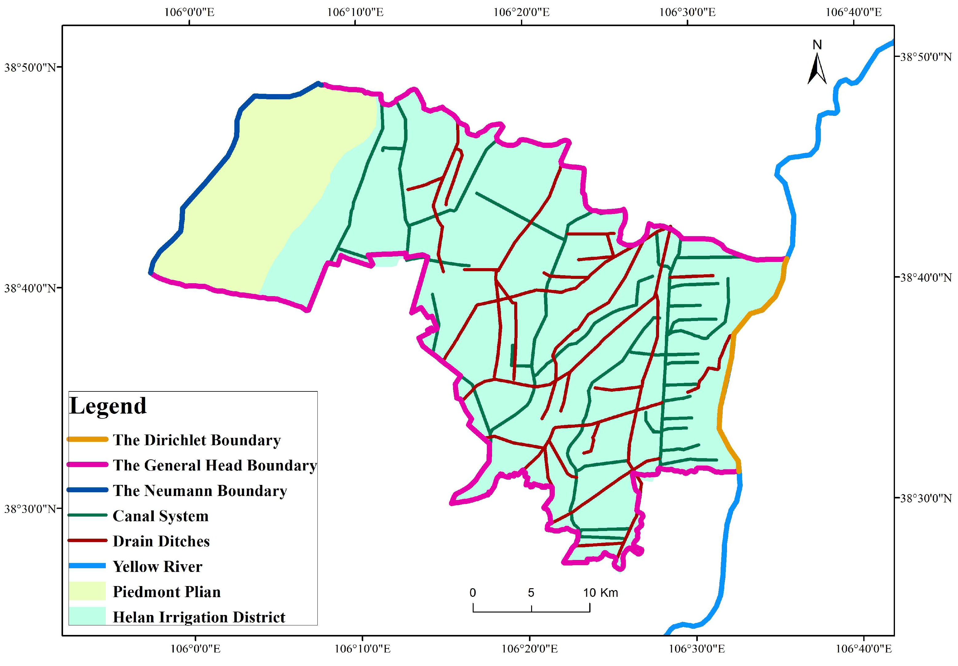
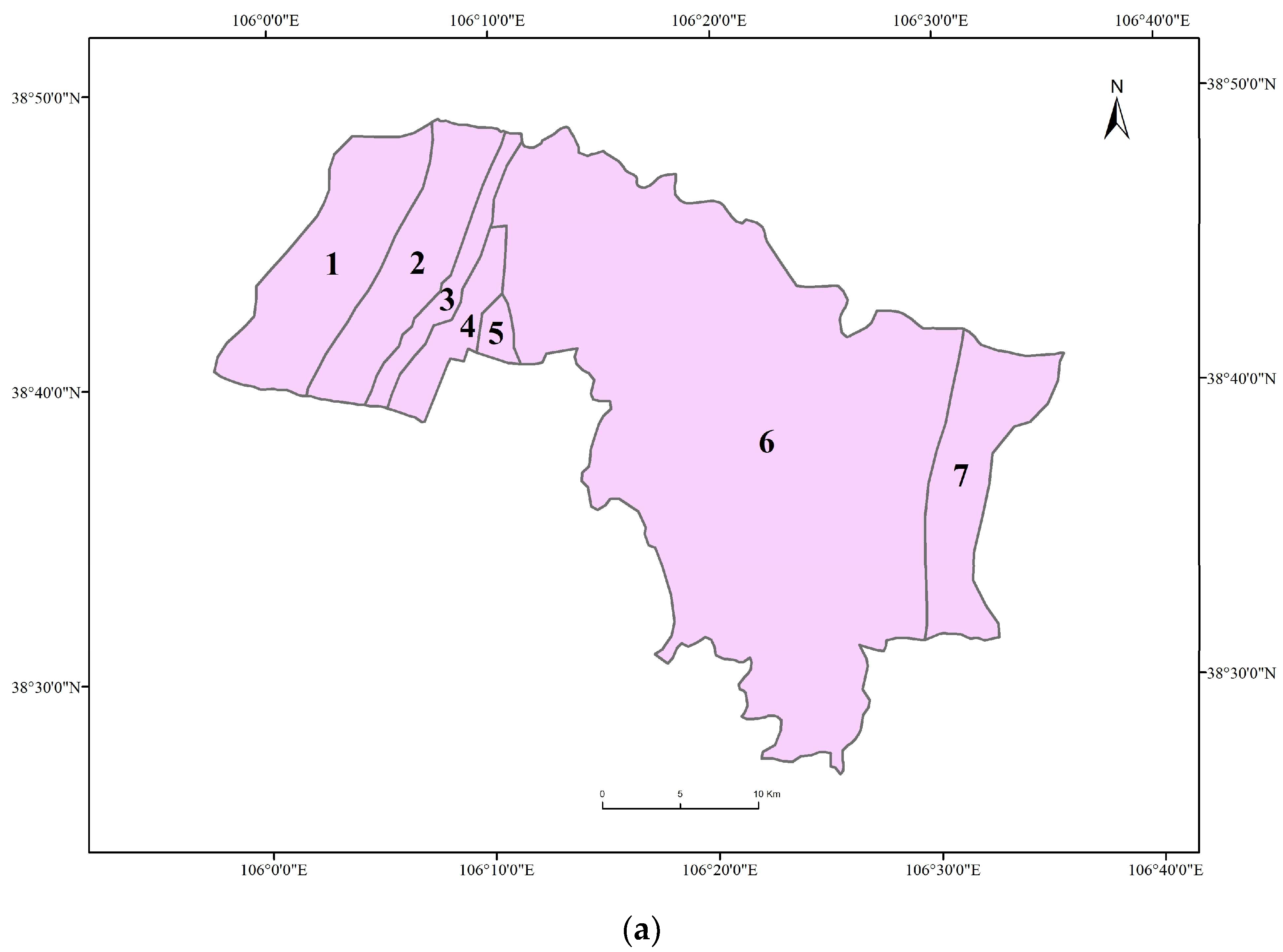
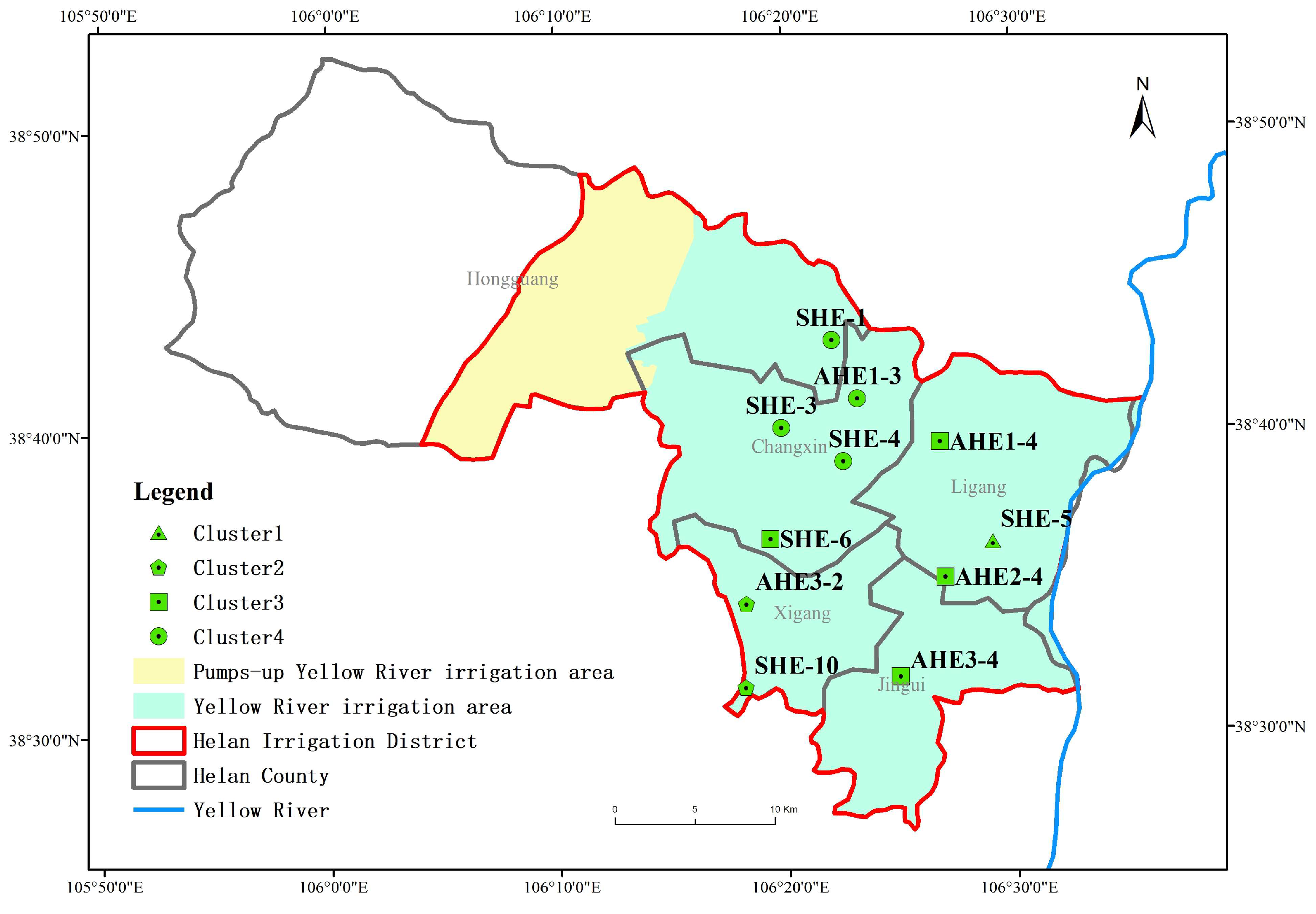
2.1. Study Area and Datasets

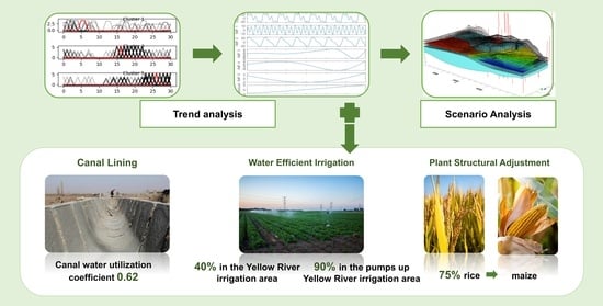
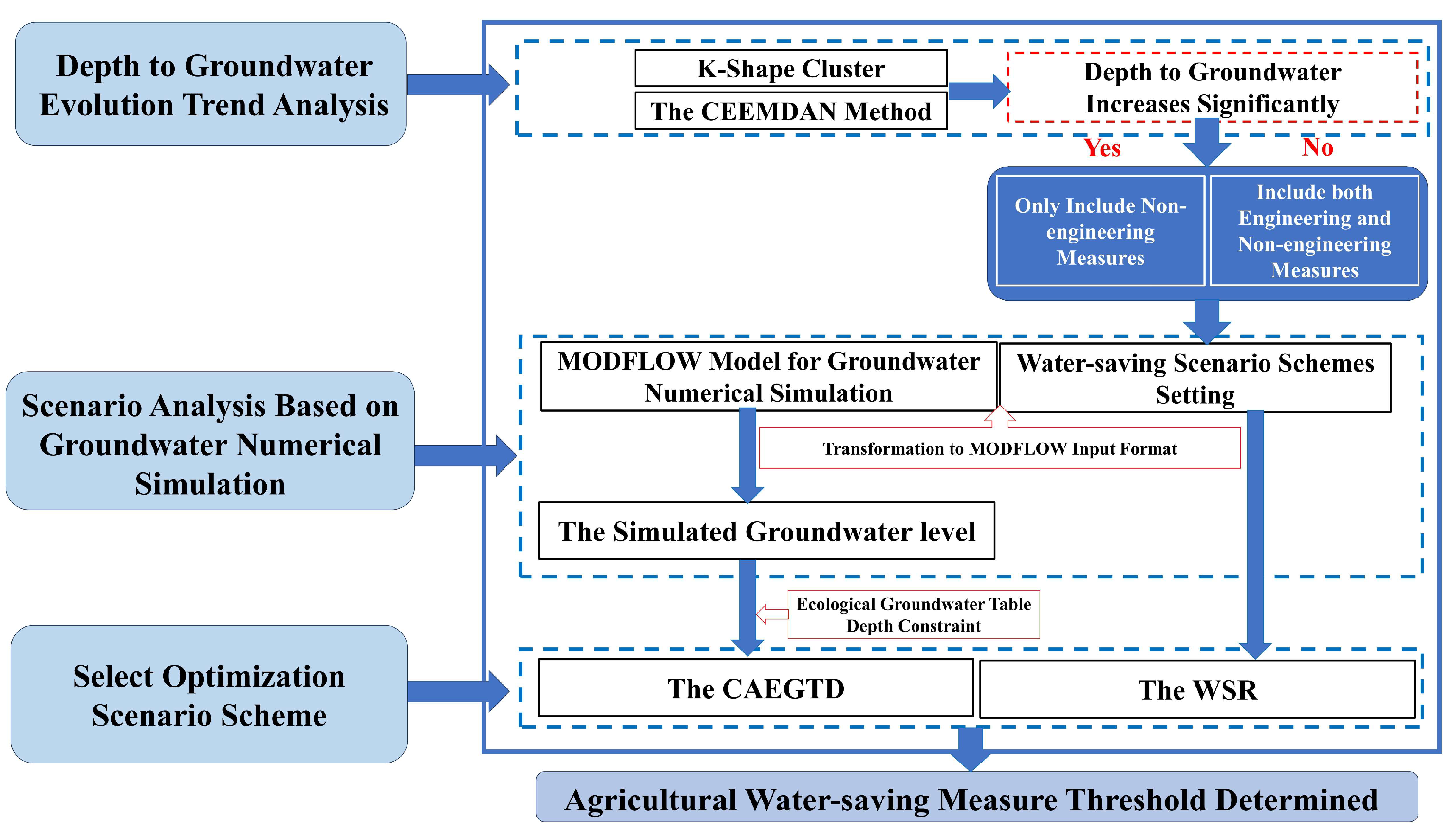
The Helan irrigation district is located in the arid region of the north-central part of Qingtongxia Yellow River Irrigation District, Ningxia Hui Autonomous Region, China, which lies at a longitude of 105°53′ to 106°36′ N and latitude of 38°27′ to 38°52′ E (Figure 1). The precipitation in this region is characterized by a modest annual average of 212 mm, while the evaporation exhibits a substantial annual average of 1313 mm. The study area is characterized by a lack of natural surface runoff, with the surface water system primarily composed of artificial channels and drainage ditches. The availability of surface water resources is limited. The irrigation of regional agriculture is predominantly dependent on artificial channels to draw water from the Yellow River on the western border. The topography of the Helan irrigation district exhibits a southwest-to-northeast gradient, characterized by higher elevations in the southwest and lower elevations in the northeast. The elevation varies within the range of 1102–1122 m. The western part is characterized by higher terrain and serves as a “pumps-up Yellow River irrigation area”. The construction of a water-lifting project in this region is necessary to utilize the water from the Yellow River for irrigation purposes. The eastern part corresponds to the “Yellow River irrigation area”, which is an artesian irrigation area (Figure 1). The primary crops cultivated include rice, vegetables, wheat, and corn. Notably, vegetables and rice, which have high water requirements, constituted a significant proportion of the crop cultivation area in 2017 at 26.16% and 14.42%, respectively [39]. The demand for agricultural water is substantial; however, the annual decrease in water supply from the Yellow River exacerbates the evident disparity between the availability and demand of regional water resources. The spatial and temporal distribution of water resources exhibits non-uniformity, with the coexistence of water scarcity and secondary salinization in this region.

The monthly DTG data of 11 observation wells were acquired from the Ningxia Hydrology and Water Resources Survey Bureau. The DTG data from January 1995 to December 2018 were used for analyzing the evolution trend of DTG via the k-Shape cluster and CEEMDAN method. The DTG data from January 2016 to December 2018 were employed for identifying and validating groundwater numerical simulation. The borehole data on the geological structure of the MODFLOW model were obtained from a geological cloud database (https://zk.cgsi.cn/ (25 June 2022)), while the hydrogeological parameter data encompass the permeability coefficient and specific yield of the aquifer, precipitation infiltration recharge coefficient, canal system leakage recharge coefficient, and irrigation infiltration recharge coefficient, which were sourced from the results of the third water resources survey and evaluation in Ningxia Hui Autonomous Region. Data related to water-saving measures include the acreage of the crop, water-efficient irrigation area, and canal water utilization coefficient from the Ningxia Statistical Yearbook (http://nxdata.com.cn/files_nx_pub/html/tjnj/2018/indexfiles/indexch.htm?1=1 (10 August 2022)) and “Ningxia Hui Autonomous Region Water Conservancy Statistical Bulletin” (http://slt.nx.gov.cn/xxgk_281/fdzdgknr/gbxx/sltjgb/202105/t20210507_2824670.html (10 August 2022)). The climate data, the amount of water diverted from the Yellow River from 2016 to 2018, were obtained from Ningxia Water Resources Bulletin (http://slt.nx.gov.cn/xxgk_281/fdzdgknr/gbxx/szygb/ (10 August 2022)) and a monthly precipitation data set with a 1 km resolution in China from 1960 to 2020 [40]. The land use data for 2017 were obtained from the land cover dataset [41]. The water level data of the Yellow River at each hydrological station were obtained from the China Hydrological Yearbook for the years 2016–2018.

2.2. Methodology

As shown in Figure 2, this research was carried out in three phases. In the first phase, the evolution trends of DTG in the study area were clustered and the specific variation forms within each cluster were analyzed using statistical methods. The implementation of agricultural water-saving measures increases the regional DTG, enabling the trend of DTG to serve as a criterion for assessing the suitability of further reinforcing existing agricultural water-saving measures in the area. If there is a significant increase in the regional DTG, it is not recommended to further enhance existing engineering water-saving measures and set up water-saving scenario schemes that exclusively incorporate non-engineering measures. Instead, it is recommended to intensify both existing engineering and non-engineering water-saving measures.

In the second phase, we established the groundwater numerical model using MODFLOW, which can reflect the actual groundwater level dynamics within the study area and set up various water-saving scenario schemes.

The following technique is employed to facilitate the conversion of various water-saving schemes into groundwater recharge terms within the MODFLOW model. The water demand and supply for each water-saving scenario scheme were calculated based on the established agricultural irrigation water allocation model [42]. The water supply represents the amount of water diverted from the Yellow River in the canal system. The groundwater recharge amount from canal system leakage was obtained by multiplying the water diversion of the canal system with the canal leakage recharge coefficient, and it was incorporated into the MODFLOW model as “Specified Flow”. The water supply multiplied by the canal water utilization coefficient is the amount of farmland irrigation. This quantity was then multiplied by the coefficient for irrigation infiltration recharge, representing the amount of groundwater recharge through irrigation. It was transformed into a recharge rate format and incorporated into the MODFLOW model using the RCH package. The meteorological conditions of precipitation, evaporation, and groundwater exploitation in the model remained unchanged. Therefore, the dynamics of groundwater level are primarily influenced by the recharge of groundwater from canal system leakage and irrigation infiltration. Subsequently, the groundwater numerical simulation of each water-saving scenario scheme was carried out to obtain the groundwater level after the implementation of each scheme.

In the third phase, two evaluation indices, namely the CAEGTD, and WSR, were employed to identify the optimal water-saving scenario scheme and determine the threshold values for agricultural water-saving measures.

2.3. Statistical Methods for DTG Evolution Trend Analysis

2.3.1. K-Shape Clustering

K-Shape clustering adopts a normalized version of the cross-correlation measure to compute cluster centroids, which are used in every iteration to update the assignment of time series to clusters. With replies to a scalable iterative refinement procedure, k-Shape creates homogeneous and well-separated clusters. Given a set of n observations, $X=\left\{\overrightarrow{x_1},\dots ,\overrightarrow{x_n}\right\}$, where $\overrightarrow{x_i}\in R^m$ and the number of clusters k < n, the objective is to partition X into k pairwise-disjoint clusters, $P=\left\{p_1,\dots , p_k\right\}$ [38]. The k-Shape clustering algorithm performs two important steps:

(1) $\overrightarrow{x}=\left(x_1,\dots ,x_m\right)$ and $\overrightarrow{y}=\left(y_1,\dots ,y_m\right)$, which are two sequences in the dataset, which can be properly aligned or not. Shape-based distance (SBD) is calculated to measure time series similarity, where the SBD is as follows:

$$\mathrm{SBD}\left(\overrightarrow{x},\overrightarrow{y}\right)=1-\underset{\omega }{\max }\left(\frac{C{C}_{\omega }\left(\overrightarrow{x},\overrightarrow{y}\right)}{\sqrt{R_0\left(\overrightarrow{x},\overrightarrow{x}\right)·R_0\left(\overrightarrow{y},\overrightarrow{y}\right)}}\right)$$

(1)

where $C{C}_{\omega }\left(\overrightarrow{x},\overrightarrow{y}\right)$ is the cross-correlation sequence with length 2m − 1, defined as follows:

$$C{C}_{\omega }\left(\overrightarrow{x},\overrightarrow{y}\right)=R_{\omega -m}\left(\overrightarrow{x},\overrightarrow{y}\right), \omega \in \left\{1,2,\dots ,2m-1\right\}$$

(2)

$$R_{\omega -m}\left(\overrightarrow{x},\overrightarrow{y}\right)=\{\begin{array}{c}{\displaystyle \sum }_{l=1}^{m-k}{x}_{l+k}·y_l, k\ge 0\\ R_{-k}\left(\overrightarrow{y},\overrightarrow{x}\right), k<0\end{array}$$

(3)

where ω is the position at which $C{C}_{\omega }\left(\overrightarrow{x},\overrightarrow{y}\right)$ is maximized; m is the time series length.

SBD takes values between 0 and 2, with 0 indicating perfect similarity for time series sequences.

(2) Based on the principle of minimizing the sum of squares of the SBD from each sequence in the cluster to the centroid, the centroid ${\overrightarrow{{\mu }_k}}^{*}$ is found. The centroid is an average sequence in the context of clustering that is defined as follows:

$${\overrightarrow{{\mu }_k}}^{*}=\underset{\overrightarrow{{\mu }_k}}{\mathrm{argmax}}{{\displaystyle \sum }}_{\overrightarrow{x_i}\in P_k}{\left(\frac{{\max }_{\omega }C{C}_{\omega }\left(\overrightarrow{x_i},\overrightarrow{{\mu }_k}\right)}{\sqrt{R_0\left(\overrightarrow{x_i},\overrightarrow{x_i}\right)·R_0\left(\overrightarrow{{\mu }_k},\overrightarrow{{\mu }_k}\right)}}\right)}^2$$

(4)

Clustering is achieved by loop iteration. In every iteration, k-Shape performs two steps: (i) the algorithm updates the cluster memberships by comparing each time series to all computed centroids and by assigning each time series to the cluster of the closest centroid; (ii) the cluster centroids are updated to reflect the changes in cluster memberships in the previous step. k-Shape clustering repeats these two steps until either no change in cluster membership occurs or the maximum number of iterations allowed is reached. In this paper, the tslearn package in Python is utilized to implement the k-Shape clustering of DTG data [43].

2.3.2. The Complete Ensemble Empirical Mode Decomposition with Adaptive Noise (CEEMDAN) Method

The CEEMDAN method adds specific white noise to the remaining components of each scale of the decomposition and obtains the intrinsic mode function (IMF) by calculating the unique residual. The trend of the ultimate residual after the separation of each IMF from the original signal is the trend of the original signal [29]. Specific steps include the following:

(1) Gaussian white noise is added to the original signal, s(t), N rounds of EMD decomposition are performed, and then the average value is taken to obtain their first modes, as follows:

$$IM{F}_1\left(t\right)=\frac{1}{N}{{\displaystyle \sum }}_{i=1}^N{E}_1\left(s\left(t\right)+{\epsilon }_0{\omega }^i\left(t\right)\right)$$

(5)

where $E_i(·)$ is the i-th mode generated via the EMD decomposition of the original signal s(t); ${\omega }^i$ is Gaussian white noise; $\epsilon$ is the proportion of noise added in each decomposition step.

(2) At the first stage (k = 1) the first residue is calculated, as in Equation (6):

$$r_1\left(t\right)=x\left(t\right)-IM{F}_1\left(t\right)$$

(6)

(3) Realizations $r_1\left(t\right)+{\epsilon }_1{E}_1\left({\omega }^i\left(t\right)\right)$, $i=1,\dots , N$, are decomposed until their first EMD mode, and the second mode is defined as follows:

$$IM{F}_2\left(t\right)=\frac{1}{N}{{\displaystyle \sum }}_{i=1}^N{E}_1\left(r_1\left(t\right)+{\epsilon }_1{E}_1\left({\omega }^i\left(t\right)\right)\right)$$

(7)

(4) For k = 2, …, K, the k-th residue is calculated as follows:

$$r_k\left(t\right)=r_{k-1}\left(t\right)-IM{F}_k\left(t\right)$$

(8)

(5) Realizations $r_k\left(t\right)+{\epsilon }_k{E}_k\left({\omega }^i\left(t\right)\right)$, $i=1,\dots ,N$, are decomposed until their first EMD mode, and the (k + 1)-th mode is defined as follows:

$$IM{F}_{\left(k+1\right)}\left(t\right)=\frac{1}{N}{E}_1\left(r_k\left(t\right)+{\epsilon }_k{E}_k\left({\omega }^i\left(t\right)\right)\right)$$

(9)

(6) Step 4 is revisited for the next k.

Steps 4 to 6 are repeated until the residue cannot be decomposed to obtain the final residue:

$$R\left(t\right)=s\left(t\right)-{{\displaystyle \sum }}_{k=1}^{K}IM{F}_K\left(t\right)$$

(10)

with K as the total number of modes. The original signal, s(t), can be expressed as follows:

$$s\left(t\right)={{\displaystyle \sum }}_{k=1}^{K}IM{F}_k\left(t\right)+R\left(t\right)$$

(11)

The trend of R(t) corresponds to the trend of the original signal.

In this paper, the pyEMD package is utilized in Python to implement the CEEMDAN method [44,45].

2.4. Scenario Analysis Based on Groundwater Numerical Simulation

2.4.1. Groundwater Numerical Simulation Model Setup

The regional hydrogeological conceptual model was developed by analyzing the hydrogeological conditions and three-dimensional groundwater flow characteristics in the study area. The groundwater mathematical model was solved, identified, and verified by using MODFLOW-USG [46].

Helan County is situated in the central region of the Yinchuan Plain, with its western boundary adjoining the fault zone at the eastern foot of Helan Mountain. On the eastern side, it is connected to the Ordos block through the Yellow River fault. The model domain includes part of the Piedmont Plain and the whole plain irrigation area in Helan County, and the area is 991.4 km². The main aquifer is quaternary pore water. In the western region of the model domain, the Piedmont section of the aquifer consists primarily of phreatic water, whereas the plain section comprises both phreatic and confined aquifers within the aquifer system. The implementation of water-saving measures in agriculture has a more immediate influence on the upper aquifer. Therefore, this study focuses on the shallow groundwater in which the aquifer floor is buried 60 m underground [47] and it is generalized into a 1-layer structure vertically in the model. According to the flow field characteristics and stratigraphic structure in the region, the western Helan Mountain frontage is defined as the Neumann boundary, the eastern Yellow River is simplified as the Dirichlet boundary, and the north–south boundary is treated as the general head boundary (Figure 3).

The groundwater flow system is generalized to a heterogeneous, isotropic three-dimensional, unsteady flow system. The mathematical model of groundwater flow can be described by the following formula:

$$\{\begin{array}{c}\frac{\partial }{\partial x}\left(K_x\frac{\partial H}{\partial x}\right)+\frac{\partial }{\partial y}\left(K_y\frac{\partial H}{\partial y}\right)+\frac{\partial }{\partial z}\left(K_z\frac{\partial H}{\partial z}\right)+W=\mu \frac{\partial H}{\partial t}\hfill \\ {H|}_{{\mathsf{\Gamma }}_1}=H\left(x,y,t\right)\hfill \\ {K\left(H-B\right)\frac{\partial H}{\partial n}|}_{{\mathsf{\Gamma }}_2}=q\left(x,y,t\right)\hfill \\ {H|}_{t=0}=H_0\left(x,y\right)\hfill \end{array}$$

(12)

where K is the permeability coefficient, m/d; K_x, K_y, and K_z represent the components of the permeability coefficient along the x axis, y axis, and z axis, respectively; K_x = K_y in this model; W is the source and sink term per unit volume, m³/(d·m²); μ is specific yield; H is groundwater level, m; H₀ is the initial groundwater level, m; B is the elevation of aquifer floor, m; q is flow rate per unit area of the Neumann boundary, m³/d; n is the inner normal on the boundary; Γ₁ is the Dirichlet boundary; Γ₂ is the Neumann boundary.

The model adopts the 0.4 km × 0.4 km dividing unit, and 6753 computational units in total are obtained. The simulation period was from January 2016 to December 2018, and was divided into 36 stress periods in months. The observed groundwater level on 1 January 2016 was taken as the initial condition for the running of the groundwater numerical model.

The parameters involved in the model primarily encompass the permeability coefficient and specific yield of the aquifer, precipitation infiltration recharge coefficient, canal system leakage recharge coefficient, and irrigation infiltration recharge coefficient. The values of these coefficients were established based on the results of the third water resources survey and evaluation in Ningxia Hui Autonomous Region. The zoning of the permeability coefficient and specific yield is illustrated in Figure 4a. The determination of the precipitation infiltration recharge coefficient value considers the lithology of the soil aeration zone, the spatial distribution of annual precipitation, and the annual depth to groundwater (Figure 4b). The determination of the irrigation infiltration recharge coefficient value considers the lithology of the soil aeration zone, the spatial distribution of the depth to groundwater during the irrigation period (April to September; November), and the irrigation system (Figure 4c). The determination of the canal system leakage recharge coefficient requires a consideration of various factors, such as the lining rate, canal length, main branch canal, lithology beneath the canal bed, and groundwater depth. It has been determined as 0.197 within this model. In addition, the limiting evaporation depth of groundwater is determined to be 3 m, as the dominant lithology of soil in the majority of the study area is clay sand.

The specific input format for each source and sink item in MODFLOW is as follows: The RCH package was used to implement precipitation infiltration and irrigation infiltration, while the EVT package simulated phreatic evaporation. “Specified Flow” inputs were used to incorporate recharge from the canal system leakage and Piedmont recharge, whereas the Yellow River was represented as a “Specified Head” input. The DRN package was applied to treat drain ditches. In the study area, the exploitation of shallow groundwater is limited to scattered instances rather than being widespread. In this model, groundwater extraction is simulated using the RCH package.

2.4.2. Water-Saving Scenario Scheme Setting

Agricultural water-saving measures include both engineering and non-engineering measures, namely canal lining, water-efficient irrigation transformation, and plant structural adjustment. It should be noted that the planting structure of crops in the region is mainly rice and vegetables with high water consumption. The planting area of rice is the largest. Therefore, the primary focus of plant structural adjustment lies in reducing the rice cultivation area and increasing the cultivation area of maize, which exhibits low water consumption.

In this study, 2017 was chosen as the baseline year, and the water-saving scenarios were set via the combination of engineering and non-engineering water-saving measures.

The baseline year situation of the Helan Irrigation District is as follows: the total planting area was 731,900 acres, including 191,430 acres of rice, 105,520 acres of vegetables, 71,220 acres of wheat, 60,300 acres of maize, 28,010 acres of intercropped maize and 275,420 acres of other crops; in terms of the water use index, the proportion of water-efficient irrigation areas to effective irrigation areas was 20.8% in the Yellow River irrigation area and 58% in the pumps-up Yellow River irrigation area; the canal water utilization coefficient is 0.605; the rice irrigation quota is 1000 m³ of irrigation water per acre of rice [48]; the WSR is 21%.

Based on the situation of the baseline year, with a focus on promoting water-saving development, the engineering water-saving measures were set as follows: (1) the canal water utilization coefficient was increased from the current 0.605 to 0.62 and 0.64; (2) the proportion of water-efficient irrigation areas to effective irrigation areas was increased to 30%, 35%, and 40% in the Yellow River irrigation area and 70%, 80%, and 90% in the pumps-up Yellow River irrigation area concerning the “Helan County Water saving Plan” [49]. The non-engineering water-saving measures were set as follows: (1) the rice planting area was reduced by 50% and 75% and changed to maize; (2) according to the “Agricultural Irrigation Water Quota of Ningxia” and the actual irrigation experience, the irrigation quota for the remaining rice area was reduced from 1000 m³ to 790 m³ of irrigation water per acre of rice. The aforementioned measures were complemented by 12 water-saving scenarios, as illustrated in

Table 1. Water-saving scenario schemes in the Helan Irrigation District.

Water-Saving Measures		Water-Saving Scenario Schemes
		Z1	Z2	Z3	Z4	Z5	Z6	Z7	Z8	Z9	Z10	Z11	Z12
Canal lining	0.62	√		√		√		√		√		√
	0.64		√		√		√		√		√		√
Water-efficient irrigation transformation	30%; 70%	√	√					√	√
	35%; 80%			√	√					√	√
	40%; 90%					√	√					√	√
Plant structural adjustment	50%	√	√	√	√	√	√
	75%							√	√	√	√	√	√

Notes: In the column “Canal lining”, the numbers denote the canal water utilization coefficient; in the column “Water-efficient irrigation transformation”, the front number denotes the proportion of water-efficient irrigation areas to effective irrigation areas in the Yellow River irrigation area and the back number denotes the proportion in the pumps-up Yellow River irrigation area; in the column “Plant structural adjustment”, the numbers denote the proportion of the rice planting area converted into one of maize planting.

. The water-saving scenario scheme indicates the comprehensive implementation of three water-saving measures. Taking Z1 as an example, the canal water utilization coefficient of Z1 is set at 0.62. In the Yellow River irrigation area, water-efficient irrigation areas account for 30% of effective irrigation areas, while in the pumps-up Yellow River irrigation area, this proportion is 70%. Additionally, there is a conversion of 50% of the rice planting area into one of maize cultivation, and the irrigation quota of rice is 790 m³ of irrigation water per acre.

2.5. Optimization Scenario Scheme Evaluation Indices

The determination of the agricultural water-saving threshold necessitates the selection of an optimal scenario scheme that exemplifies superior water-saving practices. The groundwater resources in the study area primarily depend on recharge from canal leakage and infiltration through irrigation. The implementation of agricultural water-saving measures is expected to result in a reduction in groundwater recharge and an increase in the DTG. An excessive DTG in irrigated areas will give rise to significant ecological and environmental issues. It is crucial to maintain the DTG within a rational range. The ecological groundwater table depth (EGTD) serves as a pivotal indicator for the assessment of ecosystem health in arid and semi-arid regions. In addition, the implementation of agricultural water-saving measures has effectively curtailed agricultural water demand, with the WSR serving as an instrumental index to reflect the efficacy of agricultural water conservation. Therefore, the CAEGTD and the WSR were chosen as the evaluation indices in this study. The optimal scheme is characterized by a larger CAEGTD and a smaller WSR.

The DTG of each water-saving scenario is determined by subtracting the simulated groundwater level from the surface elevation, followed by spatial interpolation to calculate the area within EGTD as CAEGTD.

The concept of EGTD refers to the dynamic range of DTG that can adequately satisfy the water requirements for plant growth and development. Its upper limit is the DTG to prevent soil salinization, and its lower limit is the DTG to avoid situations that jeopardize crop growth or lead to desertification in irrigated areas. When the DTG is less than the upper limit of EGTD, the soil is susceptible to salinization. Conversely, when it exceeds the lower limit of EGTD, it may impact the normal growth of crops or lead to soil desertification [9,50,51,52]. The determination of the EGTD is based on field investigations and a comprehensive consideration of previously obtained relevant results. According to the local crop growth period, four periods were identified for determining the EGTD in the region. As shown in

Table 2. Thresholds of the EGTD during the crop growth period in the Helan Irrigation District.

Periods	Range of the EGTD/m
	${\mathit{H}}_{\mathit{u}}^{*}-{\mathit{H}}_{\mathit{l}}^{*}$
Thawing to summer irrigation (March–April)	2.0–3.0
Crop growth period (May–August)	1.2–1.8
Cessation of irrigation to winter irrigation (September–October)	1.5–2.5
Winter irrigation until the following year’s thawing season (November–the following February)	1.5–2.2

Notes: $H_u^{*}$ denotes the upper limit of EGTD; when the DTG is less than $H_u^{*}$, the soil is susceptible to salinization. $H_l^{*}$ denotes the lower limit of EGTD; when the DTG is more than $H_l^{*}$, the soil is under soil desertification.

, during the period from thawing to summer irrigation (March to April), the EGTD is maintained at 2.0–3.0 m, resulting in a reduction in the topsoil salt content to 0.1–0.2% and controlling topsoil water content in the 0–20 cm layer at 16–18%, ensuring high crop yield without desertification [53]. During the crop growth period (May–August), the EGTD ranged from 1.2 to 1.8 m, meeting the normal water requirements of crops while maintaining a favorable ecological environment in the root soil layer; from the end of irrigation until winter irrigation (September to October), a EGTD of 1.5–2.5 m was maintained primarily to minimize the soil salt return rate. Similarly, during winter irrigation until thawing next year (November to the following February), a EGTD of 1.5–2.2 m was maintained by controlling the DTG at the freezing onset to reduce salt accumulation within cultivated layers [53,54,55,56,57].

The WSR is defined in the following manner:

$$\mathrm{WSR}=\frac{WD-WS}{WD}\times 100\%$$

(13)

where WD is the total water demand of each scheme, 10⁸ m³; WS is the total water supply of each scheme, 10⁸ m³.

3. Results

3.1. Classification of Wells Based on Cluster Analysis

The elbow method refers to the point at which the ‘Distortion’ abruptly decreases and then stabilizes, indicating the optimal number of clusters. According to the elbow method of clustering analysis, the 11 groundwater observation wells in the Helan Irrigation District can be classified into four clusters by using the k-Shape method (Figure 5). The DTG variation in the observation wells within each cluster exhibits a consistent trend from January 1995 to December 2018 (Figure 6).

The groundwater observation wells within each cluster exhibit distinct spatial zoning characteristics. Cluster 1 comprises well SHE-5, situated in the eastern part of the irrigated area and adjacent to the Yellow River. Cluster 2 consists of wells AHE3-2 and SHE-10, located in the southwest near the urban area of Yinchuan. Cluster 3 encompasses wells AHE1-4, AHE2-4, AHE3-4, and SHE-6, positioned in the central region of the irrigated area. Lastly, cluster 4 includes wells AHE1-3, SHE-1, SHE-3, and SHE-4, which are found in the northwest (Figure 7).

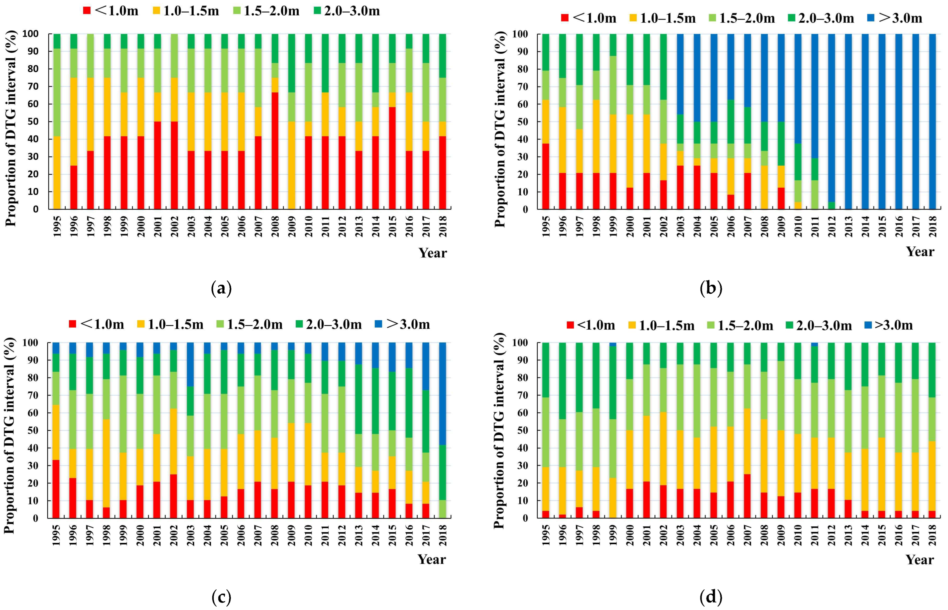
3.2. Trend Analysis of Depth to Groundwater

The trends in monthly average DTG data for four cluster observation wells from 1995 to 2018 were analyzed using the CEEMDAN method. The proposed method utilizes the DTG data as a time series signal and decomposes it into multiple intrinsic mode functions (IMFs) along with a residual signal. Notably, the residual signal exhibits trends consistent with the original signal. The results indicate that the DTG variation in cluster 1 remains essentially stable, while in cluster 2 it is stable before 2003 and exhibits a rapid increase thereafter. In cluster 3, the DTG variation remains stable before 2003 and shows a gradually increasing trend afterward. As for cluster 4, it experienced a slow decrease from 1995 to 2003 followed by an increase after that period (Figure 8). Furthermore, the evidence provided by the DTG interval proportions of these four clusters from 1995 to 2018 supports the aforementioned findings (Figure 9).

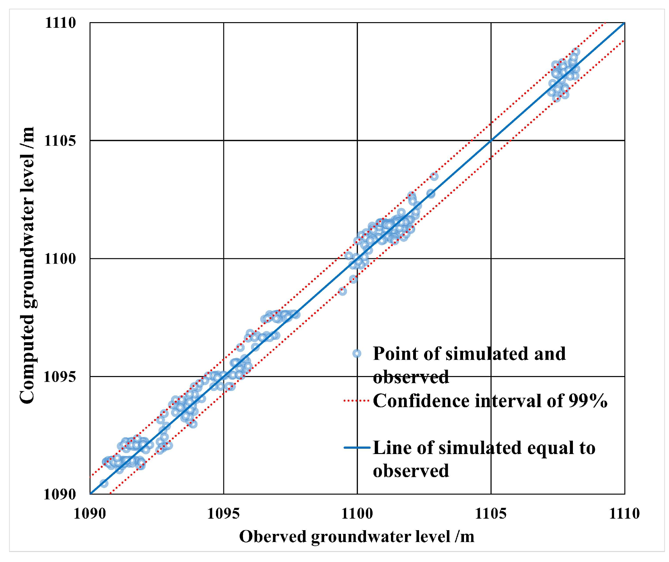
3.3. Identification and Validation of Groundwater Numerical Model

The MODFLOW model employs January 2016 to December 2017 as the identification period and January to December 2018 as the verification period. The hydrogeological parameters of the model were adjusted to minimize the discrepancy between the observed and computed groundwater levels of 11 groundwater observation wells from January 2016 to December 2017, ensuring an error tolerance of 0.5 m. The hydrogeological parameter zoning and adjusted parameter values are illustrated in Figure 4a and

Table 3. The parameter values after identification.

Parameters Zone	Kx = Ky m/d	Kz m/d	Sy
1	35	0.0023	0.3
2	25	0.0018	0.25
3	3	0.00003	0.1
4	12	0.00012	0.2
5	7.2	0.00072	0.18
6	7	0.0007	0.16
7	10	0.001	0.15

Notes: K_x and K_y denote the horizontal permeability coefficients, K_z denotes the vertical permeability coefficient, and S_y represents the specific yield.

.

All source and sink items from January to December 2018 are inputted into the model to assess the suitability of the selected parameters. The comparison between the observed and simulated groundwater levels of some observation wells is shown in Figure 10. An error analysis was performed by employing the observed data and simulated results from 11 groundwater observation wells (Figure 11). The observed and computed values of the groundwater table level demonstrate an R² of 0.993 and an RMSE of 0.43.

February as the month with the lowest groundwater level and August as the month with the highest groundwater level in 2018 were selected as typical months, facilitating a comparative analysis of the actual and simulated flow fields of groundwater. The simulated flow field demonstrates a consistent alignment with the overall flow direction of the actual flow field, as illustrated in Figure 12. Based on the aforementioned comprehensive analysis, it can be deduced that the model provides an adequate representation of the actual groundwater dynamics within the study area. Consequently, it can be employed to simulate the groundwater dynamics under various water-saving scenario schemes.

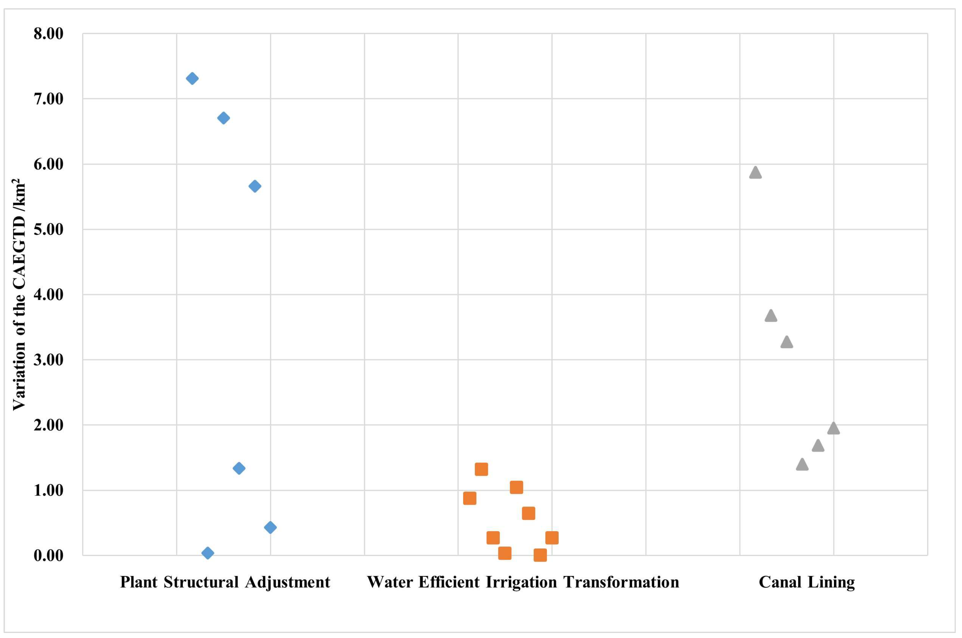
3.4. Determination of the Agricultural Water-Saving Measure Thresholds Based on Groundwater Numerical Simulation

The groundwater numerical simulation of each water-saving scenario scheme was carried out to obtain the groundwater level after the implementation of each scheme, which was calculated and spatially interpolated to obtain the CAEGTD and its average value in four periods during the crop growth period. As

Table 4. The CAEGTD within the context of water-saving scenario schemes (km²).

Water-Saving Scenario Schemes	Thawing to Summer Irrigation	Crop Growth Period	Cessation of Irrigation to Winter Irrigation	Winter Irrigation Until the Following Year’s Thawing Season	Average of Four Periods	The Growth Rate of the CAEGTD Compared to the Baseline Year (%)	WSR (%)
	March–April	May–August	September–October	November–The Following February
Baseline year	250.95	93.24	251.65	160.97	189.20	—	21.00
Z1	269.26	93.81	254.29	165.01	195.59	3.38	7.34
Z2	276.05	96.59	261.18	172.06	201.47	6.48	4.49
Z3	273.54	93.37	253.95	165.01	196.47	3.84	6.51
Z4	273.23	96.66	260.53	170.17	200.15	5.79	3.64
Z5	270.07	94.82	257.45	167.70	197.51	4.39	5.66
Z6	275.46	96.40	260.17	171.12	200.79	6.12	2.77
Z7	279.50	96.74	260.59	174.80	202.91	7.24	5.41
Z8	276.93	95.81	259.03	174.26	201.51	6.50	2.51
Z9	279.50	96.87	261.70	174.62	203.17	7.38	4.54
Z10	277.66	96.17	258.82	173.27	201.48	6.49	1.62
Z11	279.55	97.13	260.92	175.09	203.17	7.38	3.66
Z12	276.78	95.71	258.59	173.79	201.22	6.35	0.71

shows, compared with the baseline year, the implementation of comprehensive agricultural water-saving measures increased the CAEGTD and its average value in four periods during the crop growth period and decreased the WSR. However, compared with different schemes, the WSR and the CAEGTD did not show a single changing trend with the strengthening of water-saving measures. The WSR always showed a decreasing trend, while the CAEGTD increased first and then decreased. The findings suggest that the advancement in implementing agricultural water-saving measures may result in an abnormal groundwater level, underscoring the crucial need to establish thresholds for such measures.

According to the average value of the CAEGTD throughout the entire crop growth period, it was noteworthy that both the Z9 and Z11 schemes exhibit the highest values, reaching 203.17 km². The comparison between the Z11 and Z9 schemes revealed that the CAEGTD values of the Z11 scheme, during three distinct periods—thawing to summer irrigation (March–April), crop growth period (May–August), and winter irrigation until the next year before thawing (November–February)—were found to be 279.55 km², 97.13 km², and 175.09 km², respectively. Notably, all these values were observed to be larger than those obtained from the Z9 scheme. The WSR of the Z11 scheme was 3.66%, which was lower than that of the Z9 scheme at 4.54. Additionally, in comparison to the baseline year’s WSR of 21%, significant mitigation has been achieved in the agricultural water shortage. Therefore, the Z11 scheme is deemed as the optimal approach. The thresholds for implementing agricultural water-saving measures are as follows: a canal water utilization coefficient of 0.62; the proportion of water-efficient irrigation areas to effective irrigation areas accounting for 40% in the Yellow River irrigation area and 90% in the pumps-up Yellow River irrigation area; and a reduction of 75% in the rice planting area.

4. Discussion

The monthly average values of observed DTG from 1995 to 2018 for the four cluster observation wells were further analyzed to examine the annual dynamics of DTG. As shown in Figure 13, the annual dynamics of DTG in the Helan Irrigation District are primarily influenced by agricultural irrigation. The hydrological characteristics of the region are distinguished by the influence of spring and winter irrigation, with a shallow DTG from May to August and November. Furthermore, in the analysis of water-saving scenario schemes, the CAEGTD values for each scheme indicated a higher magnitude during the thawing to summer irrigation period (March–April) compared to the stopping irrigation to winter irrigation period (September–October), followed by winter irrigation until the next year before thawing (November–February), and finally, during the crop growth period (May–August). This phenomenon also signifies the impact of irrigation on groundwater levels, wherein substantial recharge from irrigation occurs during May to August and November, subsequently leading to a shallower DTG. The investigations conducted by ZHAI et al. [9], CHENG et al. [50], Ruan et al. [58,59,60], and LUO et al. [60] in the Qingtongxia Yellow River Irrigation District and on the Yinchuan Plain also demonstrate that irrigation significantly influences the annual groundwater dynamics in the region, resulting in a decrease in DTG during the irrigation period and an increase during the non-irrigation period. The annual dynamics of DTG also support that the implementation of agricultural water-saving measures has a significant impact on groundwater dynamics in the Helan Irrigation District.

JIANG et al. [61] posited that the quantity of yellow water diversion constituted the primary influencing factor on DTG fluctuations in the Qingtongxia Irrigation area. Meanwhile, FAN et al. [62] contended that variations in DTG within Pingluo County’s high- and middle-DTG distribution areas were predominantly influenced by yellow water diversion quantities, thereby substantiating that dynamic changes in DTG within the study region were primarily driven by canal leakage and irrigation infiltration recharge. The analysis conducted by ZHAI et al. [9] and Li et al. [59] further corroborates these findings regarding the contribution rates of driving factors on DTG. Therefore, the implementation of agricultural water-saving measures has resulted in a reduction in canal leakage and recharge through irrigation, leading to a gradual increase in DTG. However, the increased amplitude and pattern of DTG exhibit variations in regions where the four clusters are situated. LUO et al. [60] classified the dynamic types of groundwater in Yinchuan Plain into runoff type, rainfall–evaporation type, irrigation type, and exploitation type and investigated their spatial distribution. The findings indicate that the DTG remains stable for the runoff, rainfall–evaporation, and irrigation types; however, it progressively increases over time for the exploitation type. In this study, cluster 1 and cluster 3 are situated within the area of the irrigation type, while cluster 4 is located in the zone characterized by the rainfall–evaporation type, and cluster2 is positioned within the exploitation type zone. The variation trend of the DTG in each cluster aligns with the findings reported by LUO et al. [60]. Furthermore, the phenomenon suggests that the DTG evolution trend in the irrigated area is generally influenced by agricultural water-saving measures; however, the dominant factors vary across different regions, which may be attributed to regional characteristics. The region in which cluster 1 is situated lies in close proximity to the Yellow River. According to the data from 2008 to 2018 at two hydrological stations in Gaoren Town and Shiba, regarding the Yellow River level, it can be observed that the variation range remains within a margin of 1 m. The influence of the Yellow River weakens the evolutionary trend of DTG in cluster 1. Cluster 2 is located near the Yinchuan urban area. The escalating extraction of groundwater for urban and industrial purposes has accelerated the declining trend of DTG in this region. The DTG in the area where the 3 and 4 clusters are located generally exhibits a consistent increasing trend, although the specific variation pattern is likely influenced by factors such as water conservation practices and irrigation techniques employed during each year. Further investigation is warranted to comprehensively understand these dynamics. The water-saving planning of irrigated areas should take into account the regional DTG characteristics to determine appropriate water-saving measures.

The impact of canal lining on DTG variation is generally greater than that of planting structure adjustment and water-efficient irrigation transformation, as indicated by the simulation results of water-saving scenario schemes (Figure 14). The amount of groundwater recharged by canal leakage is approximately twice that of groundwater recharged by irrigation infiltration [8,9], thus emphasizing the significant impact of canal system lining on DTG. The aforementioned findings should be taken into consideration when discussing the appropriate water-saving measures in regions where various clusters are located. The distribution areas of clusters 1 and 3 are the primary regions for rice cultivation in the Helan Irrigation District, warranting prioritized attention towards plant structural adjustment within these two areas. Priority should be given to the implementation of canal lining in the distribution area of cluster 4. The implementation of water-saving irrigation transformation has a limited impact on the change of CAEGTD while effectively reducing the WSR. Considering the regional variations in DTG changes during implementation becomes less crucial, thus prioritizing its overall application across regions. The WSR of Z11 is lower than that of Z9 in the two relatively better schemes, while the CAEGTD remains unchanged, which also supports the previous analysis. The distribution area of cluster 2 should also prioritize water conservation in both domestic and industrial sectors, aiming to reduce groundwater exploitation and effectively counteract the excessive deepening of the DTG. The thresholds of agricultural water-saving measures in each cluster distribution area warrant further investigation.

5. Conclusions

This study determined the agricultural water-saving measure threshold by employing a methodology that integrated trend analysis and scenario analysis based on groundwater numerical simulation. The following conclusions can be drawn:

(1) The 11 groundwater observation wells can be categorized into four clusters using k-Shape clustering: cluster 1 is situated near the Yellow River; cluster 2 is located adjacent to the urban area of Yinchuan; cluster 3 is positioned within the central region of the irrigation district; and cluster 4 is situated in the northwestern part of the irrigation district.

(2) Via the CEEMDAN method, the DTG variation of cluster 1 remains relatively stable over 24 years; cluster 2 exhibits stability before 2003, followed by a rapid increase thereafter; cluster 3 demonstrated stability before 2003 and subsequently displayed a gradual upward trend; cluster 4 experienced a slow decline from 1995 to 2003, but underwent an increase post-2003.

(3) The average DTG in most areas of the Helan Irrigation District remains below 2 m, with minimal inter-annual fluctuations. Therefore, agricultural water-saving measures should be strengthened and water-saving schemes should encompass both engineering and non-engineering measures.

(4) The Z11 scheme exhibits the highest average value of the CAEGTD, measuring 203.17 km², throughout the entire crop growth period, accompanied by a lower WSR of 3.66%.

(5) The thresholds for implementing agricultural water-saving measures are as follows: the canal water utilization coefficient is set at 0.62; the proportion of water-efficient irrigation areas to effective irrigation areas should be 40% in the Yellow River irrigation area and 90% in the pumps-up Yellow River irrigation area; additionally, a reduction of 75% in the rice planting area is targeted.

The consideration of temporal and spatial trends in groundwater depth is crucial for developing appropriate water-saving strategies. It is noteworthy that the establishment of water-saving scenarios in this study is based on the overall DTG trend, allowing for a comprehensive determination of regional agricultural water-saving thresholds. Since the DTG trend varies among different clusters, further research is needed to determine agricultural water-saving thresholds in each region and develop more targeted strategies based on local conditions.

References

1. Yue, W.; Meng, K.; Hou, K.; Zuo, R.; Zhang, B.-T.; Wang, G. Evaluating climate and irrigation effects on spatiotemporal variabilities of regional groundwater in an arid area using EOFs. Sci. Total Environ. 2020, 709, 136147. [Google Scholar] [CrossRef]
2. Zhou, X.; Zhang, Y.; Sheng, Z.; Manevski, K.; Andersen, M.N.; Han, S.; Li, H.; Yang, Y. Did water-saving irrigation protect water resources over the past 40 years? A global analysis based on water accounting framework. Agric. Water Manag. 2021, 249, 106793. [Google Scholar] [CrossRef]
3. Yue, W.; Zhao, H.; Zan, Z.; Guo, M.; Wu, F.; Zhai, L.; Wu, J. Exploring the Influences of Water-Saving Practices on the Spatiotemporal Evolution of Groundwater Dynamics in a Large-Scale Arid District in the Yellow River Basin. Agronomy 2023, 13, 827. [Google Scholar] [CrossRef]
4. Cheng, G.; Xiao, H.; Li, C.; Ren, J.; Wang, S. Water-saving eco-agriculture and integrated water resources management in Heihe River Basin, Northwest China. Adv. Earth Sci. 2008, 23, 661–665. [Google Scholar]
5. Hu, Q.; Yang, Y.; Han, S.; Wang, J. Degradation of agricultural drainage water quantity and quality due to farmland expansion and water-saving operations in arid basins. Agric. Water Manag. 2019, 213, 185–192. [Google Scholar] [CrossRef]
6. Zhang, J.; Xu, J.; Zhang, Y.; Wang, M.; Cheng, Z. Water resources utilization and eco-environmental safety in Northwest China. J. Geogr. Sci. 2006, 16, 277–285. [Google Scholar] [CrossRef]
7. Gonçalves, J.M.; Pereira, L.S.; Fang, S.X.; Dong, B. Modelling and multicriteria analysis of water saving scenarios for an irrigation district in the upper Yellow River Basin. Agric. Water Manag. 2007, 94, 93–108. [Google Scholar] [CrossRef]
8. Xu, Y.; Shao, J.; Cui, Y. Application of groundwater modeling systems to the evaluation of groundwater resources in the Yinchuan Plain. Hydrogeol. Eng. Geol. 2015, 3, 7–12. [Google Scholar] [CrossRef]
9. Zhai, J.; Dong, Y.; Qi, S.; Zhao, Y.; Liu, K.; Zhu, Y. Advances in Ecological Groundwater Level Threshold in Arid Oasis Regions. J. China Hydrol. 2021, 41, 7–14. [Google Scholar] [CrossRef]
10. Yin, X.; Feng, Q.; Zheng, X.; Wu, X.; Zhu, M.; Sun, F.; Li, Y. Assessing the impacts of irrigated agriculture on hydrological regimes in an oasis-desert system. J. Hydrol. 2021, 594, 125976. [Google Scholar] [CrossRef]
11. Porhemmat, J.; Nakhaei, M.; Altafi Dadgar, M.; Biswas, A. Investigating the effects of irrigation methods on potential groundwater recharge: A case study of semiarid regions in Iran. J. Hydrol. 2018, 565, 455–466. [Google Scholar] [CrossRef]
12. Kisekka, I.; Schlegel, A.; Ma, L.; Gowda, P.H.; Prasad, P.V.V. Optimizing preplant irrigation for maize under limited water in the High Plains. Agric. Water Manag. 2017, 187, 154–163. [Google Scholar] [CrossRef]
13. Mi, L.; Tian, J.; Si, J.; Chen, Y.; Li, Y.; Wang, X. Evolution of Groundwater in Yinchuan Oasis at the Upper Reaches of the Yellow River after Water-Saving Transformation and Its Driving Factors. Int. J. Environ. Res. Public Health 2020, 17, 1304. [Google Scholar] [CrossRef] [PubMed]
14. Zhang, M.; Wang, X.; Zhou, W. Effects of Water-Saving Irrigation on Hydrological Cycle in an Irrigation District of Northern China. Sustainability 2021, 13, 8488. [Google Scholar] [CrossRef]
15. Wang, X.; Hollanders, P.H.J.; Wang, S.; Fang, S. Effect of field groundwater table control on water and salinity balance and crop yield in the Qingtongxia Irrigation District, China. Irrig. Drain. 2004, 53, 263–275. [Google Scholar] [CrossRef]
16. Morante-Carballo, F.; Montalván-Burbano, N.; Quiñonez-Barzola, X.; Jaya-Montalvo, M.; Carrión-Mero, P. Simulation of groundwater spatial distribution influenced by agricultural water-saving in Northern Irrigation Districts. Int. J. Geoherit. 2016, 4, 70–72. [Google Scholar]
17. Shan, S.; Ni, H.; Lin, X.; Chen, G. Evaluation of Water Saving and Economy Impact for Tax Reform Policy Using CGE Model with Integrated Multiple Types of Water. Water 2023, 15, 2118. [Google Scholar] [CrossRef]
18. Yang, G.; Tian, L.; Li, X.; He, X.; Gao, Y.; Li, F.; Xue, L.; Li, P. Numerical assessment of the effect of water-saving irrigation on the water cycle at the Manas River Basin oasis, China. Sci. Total Environ. 2020, 707, 135587. [Google Scholar] [CrossRef]
19. Azizpour, A.; Izadbakhsh, M.A.; Shabanlou, S.; Yosefvand, F.; Rajabi, A. Simulation of time-series groundwater parameters using a hybrid metaheuristic neuro-fuzzy model. Environ. Sci Pollut. Res. Int 2022, 29, 28414–28430. [Google Scholar] [CrossRef]
20. Bahmani, R.; Ouarda, T.B.M.J. Groundwater level modeling with hybrid artificial intelligence techniques. J. Hydrol. 2021, 595, 125659. [Google Scholar] [CrossRef]
21. Moosavi, V.; Mahjoobi, J.; Hayatzadeh, M. Combining Group Method of Data Handling with Signal Processing Approaches to Improve Accuracy of Groundwater Level Modeling. Nat. Resour. Res. 2021, 30, 1735–1754. [Google Scholar] [CrossRef]
22. Oh, Y.-Y.; Yun, S.-T.; Yu, S.; Hamm, S.-Y. The combined use of dynamic factor analysis and wavelet analysis to evaluate latent factors controlling complex groundwater level fluctuations in a riverside alluvial aquifer. J. Hydrol. 2017, 555, 938–955. [Google Scholar] [CrossRef]
23. Liang, Q.; Wang, L.; Liu, D.; Li, G. PSO-ELM prediction model of regional groundwater depth based on EEMD. Water Resour. Hydropower Eng. 2020, 51, 45–51. [Google Scholar]
24. Rahman, A.T.M.S.; Hosono, T.; Quilty, J.M.; Das, J.; Basak, A. Multiscale groundwater level forecasting: Coupling new machine learning approaches with wavelet transforms. Adv. Water Resour. 2020, 141, 103595. [Google Scholar] [CrossRef]
25. Wu, C.; Zhang, X.; Wang, W.; Lu, C.; Zhang, Y.; Qin, W.; Tick, G.R.; Liu, B.; Shu, L. Groundwater level modeling framework by combining the wavelet transform with a long short-term memory data-driven model. Sci. Total Environ. 2021, 783, 146948. [Google Scholar] [CrossRef]
26. Yang, T.; Wang, G. Periodic variations of rainfall, groundwater level and dissolved radon from the perspective of wavelet analysis: A case study in Tengchong, southwest China. Environ. Earth Sci. 2021, 80, 1–3. [Google Scholar] [CrossRef]
27. Yosefvand, F.; Shabanlou, S. Forecasting of Groundwater Level Using Ensemble Hybrid Wavelet–Self-adaptive Extreme Learning Machine-Based Models. Nat. Resour. Res. 2020, 29, 3215–3232. [Google Scholar] [CrossRef]
28. Zhang, X.; Wu, X.; Zhao, R.; Mu, W.; Wu, C. Identifying the facts and driving factors of deceleration of groundwater table decline in Beijing during 1999–2018. J. Hydrol. 2022, 607, 127475. [Google Scholar] [CrossRef]
29. Torres, M.E.; Colominas, M.A.; Schlotthauer, G.; Flandrin, P. A complete ensemble empirical mode decomposition with adaptive noise. In Proceedings of the 2011 IEEE International Conference on Acoustics, Speech and Signal Processing (ICASSP), Prague, Czech Republic, 22–27 May 2011; pp. 4144–4147. [Google Scholar]
30. Bloomfield, J.P.; Marchant, B.P.; Bricker, S.H.; Morgan, R.B. Regional analysis of groundwater droughts using hydrograph classification. Hydrol. Earth Syst. Sci. 2015, 19, 4327–4344. [Google Scholar] [CrossRef]
31. Clark, S.R. Unravelling groundwater time series patterns: Visual analytics-aided deep learning in the Namoi region of Australia. Environ. Model. Softw. 2022, 149, 105295. [Google Scholar] [CrossRef]
32. Jeihouni, E.; Eslamian, S.; Mohammadi, M.; Zareian, M.J. Simulation of groundwater level fluctuations in response to main climate parameters using a wavelet–ANN hybrid technique for the Shabestar Plain, Iran. Environ. Earth Sci. 2019, 78, 293. [Google Scholar] [CrossRef]
33. Kayhomayoon, Z.; Ghordoyee Milan, S.; Arya Azar, N.; Kardan Moghaddam, H. A New Approach for Regional Groundwater Level Simulation: Clustering, Simulation, and Optimization. Nat. Resour. Res. 2021, 30, 4165–4185. [Google Scholar] [CrossRef]
34. Naranjo-Fernández, N.; Guardiola-Albert, C.; Aguilera, H.; Serrano-Hidalgo, C.; Montero-González, E. Clustering Groundwater Level Time Series of the Exploited Almonte-Marismas Aquifer in Southwest Spain. Water 2020, 12, 1063. [Google Scholar] [CrossRef]
35. Ning, L.; De-peng, Y.; Qiang, Y.; Qi-bin, Z.; Huan, M. Temporal and spatial variation characteristics of groundwater depth in Dengkou County. South-North Water Transf. Water Sci. Technol. 2017, 15, 49–54. [Google Scholar] [CrossRef]
36. Noori, A.R.; Singh, S.K. Spatial and temporal trend analysis of groundwater levels and regional groundwater drought assessment of Kabul, Afghanistan. Environ. Earth Sci. 2021, 80, 1–16. [Google Scholar] [CrossRef]
37. Sahoo, S.; Swain, S.; Goswami, A.; Sharma, R.; Pateriya, B. Assessment of trends and multi-decadal changes in groundwater level in parts of the Malwa region, Punjab, India. Groundw. Sustain. Dev. 2021, 14, 100644. [Google Scholar] [CrossRef]
38. Paparrizos, J.; Gravano, L. k-Shape. In Proceedings of the 2015 ACM SIGMOD International Conference on Management of Data, Melbourne, Australia, 31 May–4 June 2015; pp. 1855–1870. [Google Scholar]
39. Water Conservancy Department of Ningxia Hui Autonomous Region. Statistical Bulletin on Water Conservancy in the Ningxia Hui Autonomous Region for the Year 2017. Available online: http://slt.nx.gov.cn/xxgk_281/fdzdgknr/gbxx/sltjgb/202105/t20210507_2824670.html (accessed on 10 August 2022).
40. Qu, L.; Zhu, Q.; Zhu, C.; Zhang, J. Monthly Precipitation Data Set with 1 km Resolution in China from 1960 to 2020; Science Data Bank: Beijing, China, 2022. [Google Scholar] [CrossRef]
41. Yang, J.; Huang, X. The 30 m annual land cover datasets and its dynamics in China from 1990 to 2020 (1.0.0). Earth Syst. Sci. Data 2021, 13, 3907–3925. [Google Scholar] [CrossRef]
42. Li, S.; Yang, G.; Wang, H.; Song, X.; Chang, C.; Du, J.; Gao, D. A spatial-temporal optimal allocation method of irrigation water resources considering groundwater level. Agric. Water Manag. 2023, 275, 108021. [Google Scholar] [CrossRef]
43. Tavenard, R.; Faouzi, J.; Vandewiele, G.; Divo, F.; Androz, G.; Holtz, C.; Payne, M.; Yurchak, R.; Rußwurm, M.; Kolar, K.; et al. Tslearn, a Machine Learning Toolkit for Time Series Data. J. Mach. Learn. Res. 2020, 21, 1–6. [Google Scholar]
44. Pele, O.; Werman, M. A linear time histogram metric for improved sift matching. In Computer Vision-ECCV 2008; Springer: Berlin/Heidelberg, Germany, 2008; pp. 495–508. [Google Scholar]
45. Pele, O.; Werman, M. Fast and robust earth mover’s distances. In Proceedings of the 2009 IEEE 12th International Conference on Computer Vision, Kyoto, Japan, 29 September–2 October 2009; pp. 460–467. [Google Scholar]
46. Panday, S.; Langevin, C.D.; Niswonger, R.G.; Ibaraki, M.; Hughes, J.D. MODFLOW-USG version 1.4.00: An unstructured grid version of MODFLOW for simulating groundwater flow and tightly coupled processes using a control volume finite-difference formulation. US Geol. Surv. Softw. Release 2017, 27. [Google Scholar] [CrossRef]
47. Ningxia Groundwater Bulletin. 2015–2019.
48. Water Quota of Related Industries in Ningxia Hui Autonomous Region. 2020.
49. Helan County Water Saving Plan. 2018.
50. Cheng, X.-G.; Zhang, X.; Jiang, B.-Z. Research on appropriate water saving threshhold in Qingtongxia irrigation district of Ningxia autonomous region. J. Water Resour. Water Eng. 2010, 21, 83–86. [Google Scholar]
51. Feng, Q.; Peng, J.; Li, J.; Xi, H.; Si, J. Using the concept of ecological groundwater level to evaluate shallow groundwater resources in hyperarid desert regions. J. Arid Land 2012, 4, 378–389. [Google Scholar] [CrossRef]
52. Li, F.; Wang, Y.; Zhao, Y.; Qiao, J. Modelling the response of vegetation restoration to changes in groundwater level, based on ecologically suitable groundwater depth. Hydrogeol. J. 2018, 26, 2189–2204. [Google Scholar] [CrossRef]
53. Wang, L.H.G.; Wang, S.; Fang, S.; Zhang, H.; Yu, F.; Zhao, H. Evolution and Regulation of Hydrological and Salinity Dynamics in the Huanghe River Diversion Irrigation Areas in Ningxia; China Water&Power Press: Beijing, China, 2003; p. 158. [Google Scholar]
54. Jin, X.; Wan, L.; Zhang, Y.; Xue, Z.; Yin, Y. A Study of the Relationship between Vegetation Growth and Groundwater in the Yinchuan Plain. Earth Sci. Front. 2007, 14, 197–203. [Google Scholar] [CrossRef]
55. Sun, X.-C.; Jin, X.-M.; Wan, L. Effect of Groundwater on Vegetation Growth in Yinchuan Plain. Geoscience 2008, 22, 321–325. [Google Scholar]
56. Han, Y.; Ruan, B.; Wang, F. Estimation of suitable ecological water requirement for Yellow River irrigation area in Ningxia Autonomous Region. J. Hydraul. Eng. 2009, 40, 716–723. [Google Scholar]
57. Wang, Z.; Zheng, J.; Wang, H. Desertization Pre-Warning Model and Its Application. China Rural Water Hydropower 2004, 38, 1321–1329. [Google Scholar]
58. Ruan, B.-Q.; Han, Y.-P.; Jiang, R.-F.; Xu, F.-R. Appropriate water saving extent for ecological vulnerable area. J. Hydraul. Eng. 2008, 39, 809–814. [Google Scholar]
59. Li, J.; Zhou, Y.; Wang, W.; Liu, S.; Li, Y.; Wu, P. Response of hydrogeological processes in a regional groundwater system to environmental changes: A modeling study of Yinchuan Basin, China. J. Hydrol. 2022, 615, 128619. [Google Scholar] [CrossRef]
60. Luo, J.; Wang, W.; Duan, L.; Li, Y.; Zhang, Z. Dynamic Analysis of Groundwater Level in Yinchuan Plain. Northwestern Geol. 2020, 35, 195–204. [Google Scholar]
61. Jiang, X.; Zhang, X.; Zhang, Q.; Cheng, X. Analysis of response correlation between the Yellow River water and groundwater level in Qingtongxia irrigation district. J. Water Resour. Water Eng. 2012, 23, 148–150. [Google Scholar]
62. Fan, L.-Q.; Li, L.; Wu, X. Relationship between Soil Salinity and Groundwater Characteristics in Saline-alkali Land with High Groundwater Level of Yinbei Irrigation Area. Water Sav. Irrig. 2019, 6, 55–59. [Google Scholar]
Figure 1. Study area and the distribution of the groundwater observation wells.
Water 16 00220 g001
Figure 2. Flowchart of the present study.
Water 16 00220 g002
Figure 3. Boundary properties of groundwater model, canal system, and drain ditch distribution.
Water 16 00220 g003
Figure 4. Part of the parameters involved in the groundwater model; (a) denotes the distribution of aquifer parameters and the numbers correspond to the zone numbers assigned to the parameters, (b) denotes the distribution of the precipitation infiltration recharge coefficient, and (c) denotes the distribution of the irrigation infiltration recharge coefficient.
Water 16 00220 g004aWater 16 00220 g004b
Figure 5. Elbow figure; the ‘Distortion’ is the sum of the differences between each point and the cluster centroid after clustering.
Water 16 00220 g005
Figure 6. The centroid of 4 clusters; the curve shape represents the DTG fluctuation form of each cluster.
Water 16 00220 g006
Figure 7. Spatial distribution of the groundwater observation wells of 4 clusters.
Water 16 00220 g007
Figure 8. The CEEMDAN decompositions of 4 clusters: (a) cluster 1, (b) cluster 2, (c) cluster 3, and (d) cluster 4.
Water 16 00220 g008
Figure 9. The proportion of the DTG interval of 4 clusters: (a) cluster 1, (b) cluster 2, (c) cluster 3, and (d) cluster 4.
Water 16 00220 g009
Figure 10. Comparison of computed and observed groundwater levels in some observation wells. (a) Denotes AHE2-4, (b) denotes SHE-4, (c) denotes SHE-5, and (d) denotes SHE-6.
Water 16 00220 g010
Figure 11. Comparison of observed and computed groundwater levels.
Water 16 00220 g011
Figure 12. Comparison of actual groundwater flow field and simulated flow field. (a) Denotes February 2018, and (b) denotes August 2018.
Water 16 00220 g012
Figure 13. Average annual dynamics of DTG in 4 clusters from 1995 to 2018.
Water 16 00220 g013
Figure 14. The CAEGTD caused by a single measure change in the water-saving scenario schemes.
Water 16 00220 g014