A Low-Impact Development-Based Modeling Framework for Flood Mitigation in a Coastal Community

Abstract

Urbanization is known to increase the volume of stormwater runoff and peak flow rates, which leads to changes in the natural flow regime and increases the likelihood of flooding. Low-impact development (LID) practices seek to reduce runoff volume and peak flow and are generally considered to be a more sustainable solution for urban stormwater management. In this study, we present a systematic approach to address nuisance flooding issues in small cities and communities. As an application, the effectiveness of two LID practices, rain barrels and permeable pavements, were explored in mitigating the urban flooding problem of a highly urbanized small coastal watershed in Alabama, USA. The EPA Stormwater Management Model (SWMM) was first calibrated for water depth using data collected at multiple sites within the watershed during the 2014–2015 period. The calibrated model was then used to first identify the areas prone to flooding using design storms with 1, 2, 5-, 10-, 50-, and 100-year return periods. Floodplain maps were generated for those design storms with HEC-RAS. Next, LID options upstream of those flood-prone areas were assessed to potentially minimize the flooding risks. The results indicate that LID controls can have considerable benefits for stormwater management by reducing runoff volume (1–24%), peak flow rates (18–25%), and water depth (5–15%), potentially returning watersheds to their natural flow regimes, thereby minimizing the flooding risk in urbanized areas. However, the effectiveness of LIDs, especially for the runoff volume, quickly diminishes as the return periods of the storms increase. Rain barrels were identified as the most economical and effective LID within the drainage system.

1. Introduction

Floods are among the leading causes of large natural disasters, with an enormous impact on humans and the environment [1,2]. According to the Emergency Events Database, floods have impacted more people than any other natural disaster, accounting for 43% of the total people affected by disasters (nearly 74.6 million people per year) between 2003 and 2022 [3]. Many human lives are lost each year to flooding [4]. In 2023, 7763 deaths and more than USD 20 billion in losses were directly associated with flooding events [3]. In 2007, floods killed 3200 people in India and Bangladesh alone. In 2010, flooding killed 2200 people in Pakistan and another 1900 in China, while in 2013, an exceptionally high number of 6500 people died due to floods in India [5]. The number of major floods has doubled from 1389 to 3254, while the incidence of storms grew from 1457 to 2034 in the period 2000 to 2019 [6]. The 2024 floods in the Rio Grande do Sul State in Brazil affected over 2 million people, with 183 deaths, 806 injured people, and 478 cities affected in Brazil [7]. On average, 140 people are killed every year by floods in the United States [8]. For example, 39 people died in Eastern Kentucky, USA due to heavy rains in 2022 [9]. Flooding in the United States caused USD 7.96 billion in damages per year from 1985 to 2014 [10]. Flooding is listed as the most common and frequent natural disaster in the state of Alabama, USA, as well. This is especially the case for coastal Alabama because of its low elevation and the abundance of rainfall. In coastal regions, floods are caused by two factors: significant rain events and storm surges resulting from hurricanes. Sometimes there are compound events when the two events overlap, leading to much bigger disasters. Although the weather is the primary driver for both types of floods, land-use and cover (LULC) change, especially urbanization, can exacerbate the magnitude of floods resulting from the former cause (i.e., large storms). Extensive research has established that expansion of impervious surfaces, a hallmark of urban development, leads to more frequent and intense peak water flows in urban watersheds [11,12,13,14].

Low-impact development (LID) is an environmental principle to control runoff at the source in urban areas and their use can mitigate the adverse impacts of urbanization on hydrology and moderate flooding issues in urban areas [15,16]. LID practices are promoted as an alternative to traditional stormwater design to detain, store, infiltrate, and treat urban runoff, and therefore decrease the hydrological impacts of urban catchments [17,18,19]. They also help preserve the features of the natural environment, protect ecosystems, and maintain groundwater levels to natural conditions [20]. Consideration of LID practices for land planning is recommended since they focus on the causes instead of the symptoms of urban stormwater problems. LID designs are focused on managing a broad range of runoff attributes, such as volume, rate, duration, and water quality, whereas conventional stormwater management typically addresses only peak flows and limited water quality treatment (e.g., TSS removal) [21]. Further, traditional practices are not able to fully restore the natural flow regime in urban streams, which can result in severe erosion of the stream channels [22].

Research demonstrates that LID strategies can effectively reduce peak flow and runoff volume. However, their performance varies based on geographic location, storm characteristics, and the specific LID techniques implemented.

Table 1. Summary of some relevant LID studies in the literature.

Source	LID	Region	Results
[23]	Rainwater harvesting systems	Sicily, Italy	Reduced the extent of flooded areas by 35% for a 50 mm rainfall event
[24]	Bioretention Rain Garden	Waterford, Connecticut, USA	Runoff reductions were greater for smaller storms
[25]	Rainwater Harvesting	Genoa, Italy	The study found an average reduction of 33% for peak flow and 26% for runoff volume using SWMM model
[26]	Rainwater harvesting	Nanjing, China	Runoff volume can be reduced by 14%, 30%, and 58%, for 207 mm, 96 mm, and 50 mm rain events
[27]	Permeable Pavements	Nanjing, China	Reduction in runoff volume and peak flow by 1–40% and 7–43%
[28]	Permeable Pavements and Rain Barrels	Central Illinois, USA	Reduction in runoff by 3–47%
[29]	Permeable Pavements and Eco roof	Paola, Italy	Reduction in runoff by 45.8%
[30]	Rain gardens, permeable pavements, sunken grasslands, rain barrels, and a green roof	Tsingtao, China	The SWMM model results showed that LID implementations reduced runoff for the whole area, with reduction ratios varying from 21% to 63%.
[31]	Infiltration trench, permeable pavement, and rain barrel	Dresden, Germany	Removal rate ranging from 23% to 27%
[32]	Combination of Rain Barrel with other LIDs	Beijing, China	Reduction in runoff and peak flow by 48.59% and 67.29%, respectively

provides an overview of several relevant studies on LID implementations (adapted from [20]).

LIDs can not only help in reducing peak flows and runoff volumes but can also play crucial roles in water conservation. For example, [33] found that the rainwater harvesting system reduces the total domestic water demand by up to 26% and the constructed wetlands save up to 40% of the irrigation water demand in the Xingshi Village, northern Taiwan.

In this study, we present a systematic approach to address nuisance flooding issues in small cities and communities. We implemented this in a highly urbanized coastal watershed in southwest Alabama, USA, prone to frequent flooding due to (1) low elevation, (2) abundance of heavy rains, (3) high impervious cover, and (4) potential sea-level rise and increased storm surge. The methodology starts with locating the flood-prone zones using a calibrated urban watershed model. This is followed by identifying key upstream areas that have the highest contribution to flooding in those zones by applying a novel “flood generating area” index. Those areas were then considered as potential LID installation sites. Suitable LIDs were identified by consultation with the stakeholders based on cost and feasibility. The Storm Water Management Model (SWMM) was applied to the Toulmins Spring Branch Watershed (TSBW). The model, calibrated with water depth data at five different locations, was used to first identify the areas prone to flooding using different return period storms. Various levels of rain barrels/cisterns and permeable pavement scenarios were evaluated in areas disproportionately contributing to flooding at the flood-prone areas using the SWMM model to facilitate watershed management in TSBW. The effectiveness of tested LIDs was measured as a percent reduction in runoff volume, depth, and peak flow rate with the implementation of LID practices. The methods and results of this study can provide additional guidance for the decision-making processes related to LID practice implementation.

2. Materials and Methods

2.1. Study Area

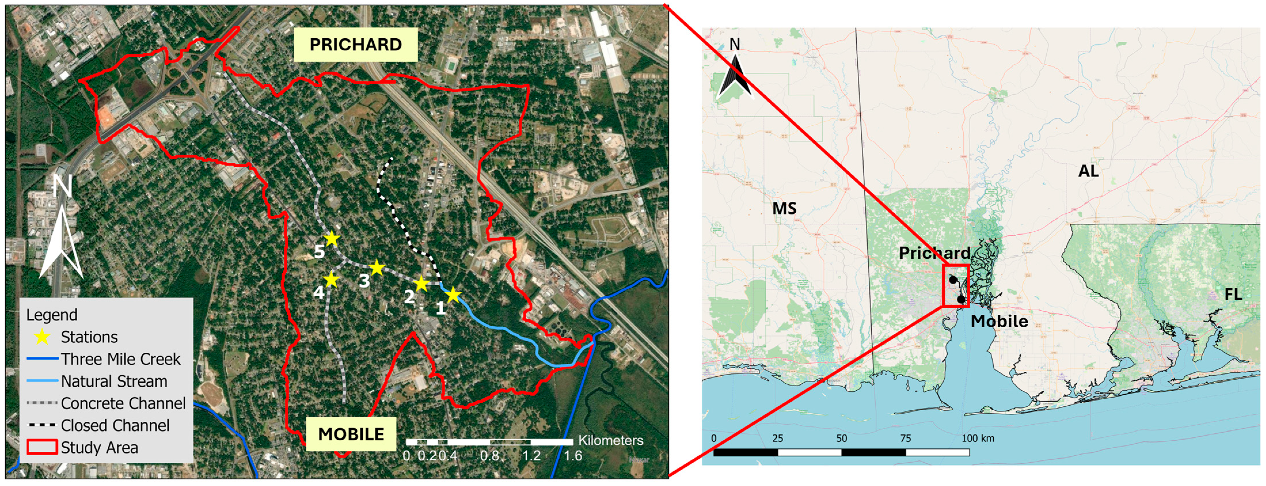
The TSBW is a sub-watershed of the Three Mile Creek watershed in Mobile County, Alabama, USA. Part of the watershed is located within the Mobile city limits and the rest is within the city of Prichard (Figure 1). Runoff generated by the TSBW flows into Three Mile Creek, which flows into Mobile Bay and eventually to the Gulf of Mexico. The choice of the watershed was driven by the complaints of the residents of the Toulmins Spring Branch (TSB) community that even 25 mm (~1 inch) rain sometimes floods their backyard and sometimes their home (Mobile Bay National Estuary Program (MBNEP) personal communication). The Mobile metro area has one of the highest volumes of rain in the U.S. (~1700 mm), and that makes the region high risk for flooding. Flood complaints often make news, such as “We’re flooding again. Every time it rains, we flood out here. A lot of times it gets so bad that it floods in the communities. But now, cars are being locked up, car parts are everywhere from the flooded water,” (https://www.fox10tv.com/2022/11/28/local-pastor-pleading-action-prichard-water-problems, accessed on 22 September 2024), and this one: “Heavy rains caused more than 430,000 of sewage overflows near Mobile. In Prichard, just north of Mobile, health officials told residents to stay away from standing water that may contain raw sewage and wash their hands or any clothing that comes in contact with overflow” [34].

The TSBW is approximately 2 km long in an east–west direction and 5 km wide in a north–south direction. The maximum elevation of the watershed is 20 m, and the minimum elevation is about 0 m above sea level. The average slope of the watershed is 1.75%. Soil types within the study area include Benndale sandy loam (41%), Harleston sandy loam (28%), and Smithon sandy loam (17%), with the additional 14% made up of miscellaneous soil types. The watershed is highly urbanized. The 2011 NLCD Land Use/Land Cover map lists the study area as 93% developed, 6% wetlands, and 1% forest and shrubs. According to estimates prepared by the U.S. Bureau of the Census, Prichard’s population was 22,659 in 2010, down from a reported population of 27,963 people in 2005, and annual per capita income was USD 12,433 in 2014. Census estimates from 2019 put the population of Prichard at 21,773. The percentage of residents in Prichard who lived below the poverty level was 35.4%. As a result, infrastructure and personal properties are often not well maintained.

2.2. Data Collection

2.2.1. Water Level and Discharge

Water level (pressure) transducers were installed at five locations (Figure 1). The pressure transducers were set to record water levels (h) at 15 min time intervals. Data were collected from 14 October 2014 to 10 November 2015 and were retrieved during site visits after significant rain events. Only three discharge measurements were taken because water levels were very low during site visits (a four-hour drive from Auburn University campus) and most significant rain events generally happened at midnight. Plus, this is a very flashy system due to the high impervious cover in the watershed, and the streams are channelized (concrete). Catching big events was thus very challenging. Discharge was measured with an Acoustic Doppler Current Profiler (ADCP). On 23 January 2015, discharge was measured at sites 1, 2, 4, and 5 only. Because of the extremely low flow, the discharge measurement was not possible at site 3 on that day. On 25 February 2015 and 15 March 2015, discharge was measured at sites 1, 2, and 5 only. Because of the limited measurements and the small size of the discharge values, we were not able to develop reliable rating curves to convert stage time series to discharge time series. Thus, model assessments were carried out with water depths.

2.2.2. Precipitation

Rainfall data in this study came from a 15 cm tipping bucket rain gauge along with the Solinst Rainlogger, which was deployed at the Prichard Municipality complex on 14 October 2014. In addition to the rain gauge, data from several other sources were also considered a potential rainfall data source. One source for precipitation data was the Community Collaborative Rain, Hail & Snow Network (CoCoRaHS) (cocorahs.org) station AL-MB-4: Mobile 2.6 WNW, which is located southwest of the TSBW. Another source was data distributed by the Center for Hurricane Intensity and Landfall Investigation (CHILI) (http://chiliweb.southalabama.edu) in Mobile (USA Campus West) station (Latitude: 30.6944° N, Longitude: 88.1944° W). In addition, Radar-based rainfall (NEXRAD stage-III) data obtained from the State Climate Office of North Carolina were also considered. The precipitation data obtained from all these stations were evaluated when the SWMM model was being calibrated. Rainfall data from all stations, when compared to the rain gauge deployed at the Prichard Municipality, exhibited high variability in precipitation through the TSBW. In general, the rain gauge data had a better correspondence with measured stage data and therefore were chosen as the precipitation data source.

Temperature data were obtained from the Center for Hurricane Intensity and Landfall Investigation (CHILI) (http://chiliweb.southalabama.edu) and were imported into the model as an external climate file. The Hargreaves equation was used to calculate potential evapotranspiration.

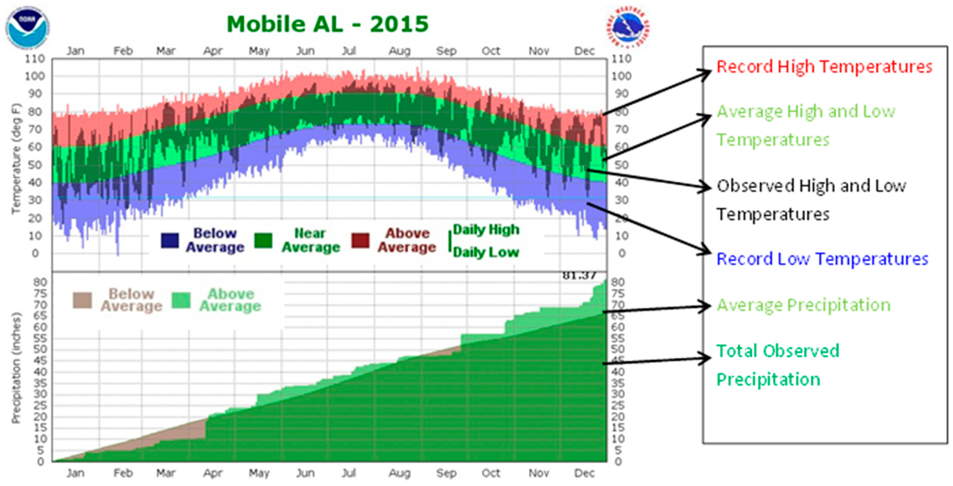
In 2015, which covered most of the study period, Mobile, AL received 2065 mm of rain, which is more than double the U.S. average rainfall and approximately 400 mm above the long-term average for Mobile, AL as shown in Figure 2 [35].

2.2.3. Stream Cross-Sections

A survey rod and level were used to derive the channel cross-section geometry of each reach. Most of the TSBW is channelized with concrete canals; only the downstream section is in natural condition (downstream of site #2 in Figure 1). The stream reaches mostly had prismatic shapes, i.e., did not vary along the reach. Channel dimensions often change when two reaches merge. The ADCP provided additional channel geometry information for the wetted parts of the channels at sites where the flow was measured.

2.3. Model Development

In this study, the Environmental Protection Agency Storm Water Management System (EPA SWMM) was used to model the streamflow and flow depth within the TSBW. The LID component of the model was later used to evaluate the potential of rain barrels and permeable pavements in flood mitigation at the TSBW. Floodplain maps were generated for different return period events to identify the areas sensitive to flooding in the watershed. The calibrated SWMM model was used to estimate peak flows for various return period storms.

The SWMM model is a dynamic rainfall-runoff simulation model used for single events or long-term simulation of runoff quantity and quality from primarily urban areas. The runoff component of SWMM operates on a collection of subwatershed areas that receive precipitation and generate runoff and pollutant loads. The routing portion of SWMM transports this runoff through a system of pipes, channels, storage/treatment devices, pumps, and regulators. SWMM tracks the quantity and quality of runoff generated within each subwatershed, pipe, and channel during a simulation period. Four functional program blocks comprise the model: Runoff, Transport, Extran, and Storage/Treatment. The blocks can be overlaid and run sequentially or separately with interfacing data files. The Runoff blocks simulate the continuous runoff hydrograph and pollutograph for each subwatershed in the drainage basin. In the Runoff block, each subwatershed surface is treated as a nonlinear reservoir with a single inflow. Surface runoff is calculated using the nonlinear storage equation, which is a combination of the continuity equation and Manning’s equation. In addition to modeling the generation and transport of runoff flows, SWMM also estimates the production of pollutant loads from land uses during storm events and routing of water quality constituents through the drainage system.

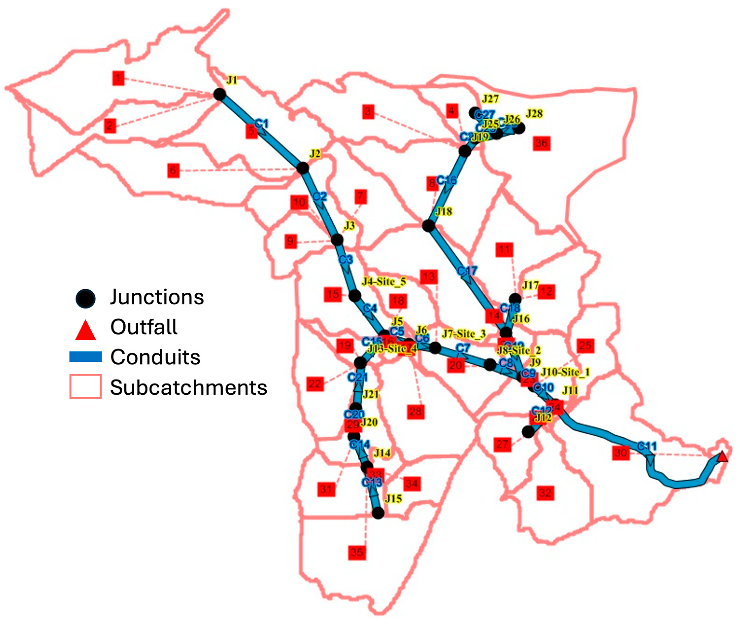
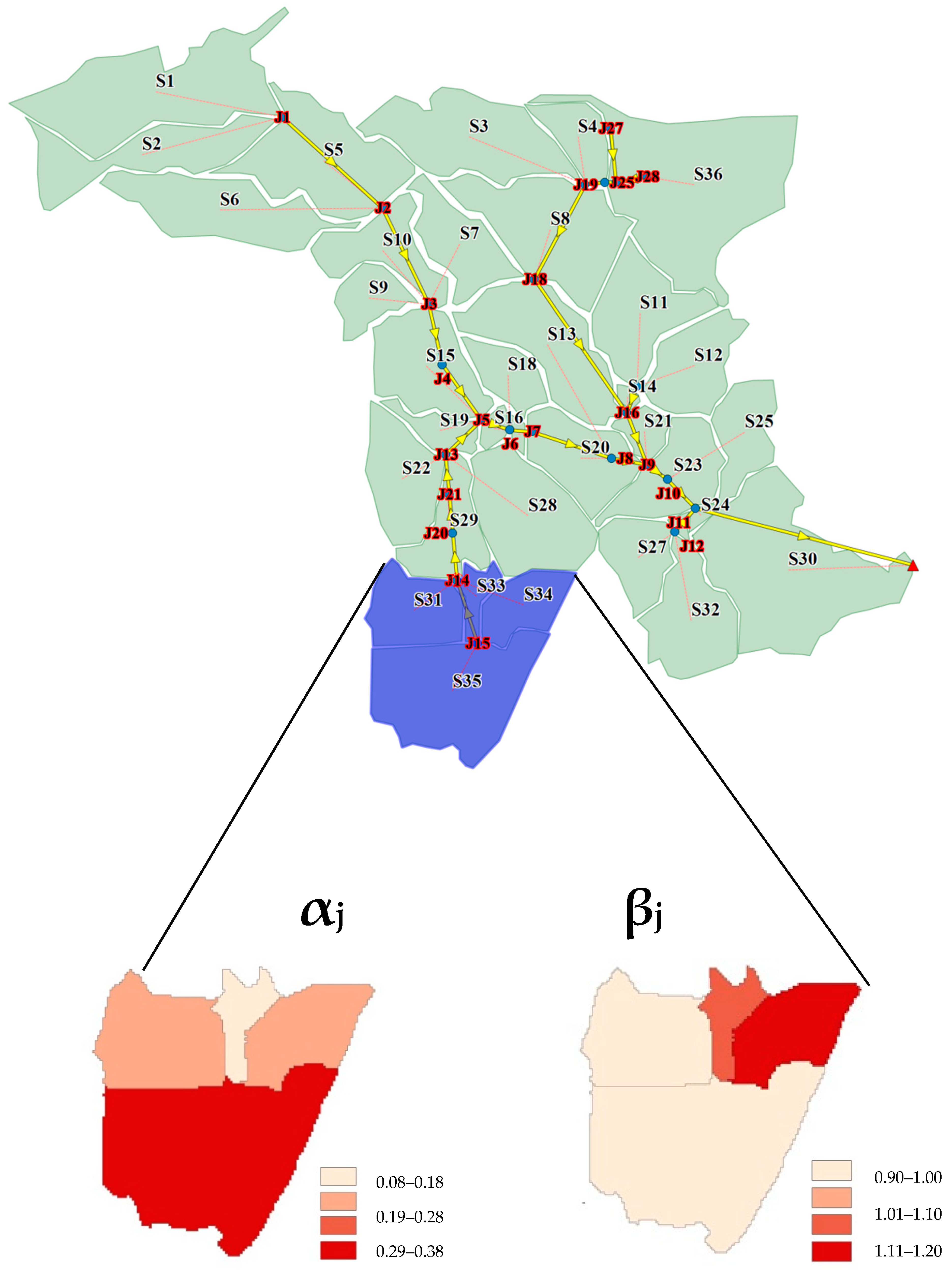
In SWMM, the study area’s water system was modeled as a set of physical components which were (i) subcatchments, (ii) junctions, (iii) conduits, and (iv) outfall. Using ArcSWAT 10.1, the TSBW boundary and its subwatersheds were delineated using a 10 m Digital Elevation Model (DEM) obtained from the United States Geological Survey National Map Service (https://apps.nationalmap.gov/downloader/, accessed on 25 September 2024). The study area was divided into 36 subcatchments, labeled from “S1” to “S36” (Figure 3). Aerial photography from 2013 at 1 m resolution was used to estimate the imperviousness of each subwatershed using geographic object-based image analysis with eCognition software Version 9.0. On average, 36.4% of surfaces within the TSBW were impervious (e.g., concrete, asphalt, roofs). Subwatershed 27, in particular, had 62.3% impervious cover, which is the highest percentage among all the subwatersheds. The main channels, which collect overland flow from the subcatchments, were identified with ArcSWAT [36]. These channels were introduced into SWMM as conduits. Within SWMM, each conduit is connected with junctions, which vary depending on invert elevation and maximum depth. A total of 25 junctions were defined, one of which was the outlet point to the Three Mile Creek. The watershed outlet was also denoted as an outfall in SWMM. The Hydrologic/Hydraulic model of TSBW by SWMM is shown in Figure 3.

The Green-Ampt method was used for modeling infiltration in SWMM. Soil texture was obtained for each soil from the USDA Natural Resources Conservation Service Web Soil Survey (https://websoilsurvey.nrcs.usda.gov). The SWMM user’s manual version 5.0 was used to determine the soil characteristics [37]. Dynamic wave routing was used since, unlike the steady flow and kinematic wave routing, dynamic wave routing can be used for channel storage, entrance/exit losses, flow reversal, pressurized flow, and the backwater effect, which is the situation in this study for the TSBW. The backwater effect can be one of the most significant effects of tides in coastal watersheds. Therefore, the impact of the tides was considered in this study. Tide time series data were downloaded from the National Oceanic and Atmospheric Administration’s (NOAA) Center for Operational Oceanographic Products and Services (https://tidesandcurrents.noaa.gov) for the outlet point of the TSBW.

2.4. LID Component in SWMM

LID practices are low-impact development controls designed to capture surface runoff and to store, infiltrate, and evaporate some of it into the atmosphere. They are considered properties of a given subwatershed in SWMM. Two generic types of LID controls are explicitly modeled in this research based on the cost and feasibility discussion with MBNEP.

• Rain barrels (RB) or cisterns are storage tanks that collect runoff from a rooftop during rainfall events and can either release or allow reuse of the rainwater during dry periods [38].
• Permeable pavement (PP) systems are dug-up areas covered with gravel and paved over with a porous concrete or asphalt mix. All rainfall directly percolates through the pavement into the gravel storage layer below it where it can infiltrate at natural rates into the site’s native soil. Block paver systems consist of impervious paver blocks placed on sand or a pea gravel bed with a gravel storage layer below. Rainfall is captured in open spaces between the blocks and conveyed to the storage zone and native soil below [38].

Permeable pavement systems can transfer the captured runoff off the site instead of letting it all infiltrate by containing optional underdrain systems in their gravel storage beds. They can be subjected to reduced hydraulic conductivity gradually due to clogging [37]. LID controls within a subwatershed in SWMM can be placed in two different ways:

• One or more LID controls can be placed in an existing subwatershed that will displace an equal amount of non-LID area from the subwatershed;
• Create a new subwatershed devoted entirely to just a single LID practice.

The first approach, which was used in the TSBW model, considered a mix of LIDs to be placed throughout a subwatershed, each treating a different portion of the runoff generated from the non-LID fraction of the subwatershed. Note that under this option, the LIDs in a subcatchment act in parallel. It is not possible to make them act in series (i.e., have the outflow from one LID control become the inflow to another LID).

Considering the possibility of both single and combined applications of LID practices, three implementation scenarios of selected LID practices were designed. The first two scenarios implemented two single LID practices (single RB and single PP), and the third scenario implemented LID combinations (RB + PP). These implementation scenarios with different installation sites and characteristics were determined based on a literature review, the SWMM design manual, and the Low Impact Development Handbook for the State of Alabama [39]. The placement of LIDs was determined based on the land-use distribution and existing condition of the study area. Rain barrels 100 gallons in size and 1500-gallon cisterns were the two feasible rainfall collection systems based on the discussion with MBNEP. In this study, we considered half of the houses had 2 × 100-gallon rain barrels, and half of them had 1500-gallon cisterns.

For rain barrels and cisterns, SWMM requires the number of rain barrels/cisterns, % of catchment they serve, % of impervious area treated, where the outflow should return to, etc. For permeable pavements, the characteristics of the pavement, soil, and storage layer should be provided. Some of the surface properties are whether there is vegetation and if there is a volume fraction, surface roughness, and slope. For the pavement layer, some of the important parameters are thickness, void ratio, impervious surface fraction, permeability, clogging factor, etc. For the soil layer, thickness, porosity, field capacity, wilting point, conductivity, and suction head need to be provided. For the storage layer, thickness, void ratio, seepage rate, and clogging factor are needed. If there was a recommendation in the Alabama LID manual, we used those; otherwise, we stuck to the recommended values in the SWMM manual.

2.5. Model Calibration

Because we had only three discharge measurements, The SWMM model parameters were calibrated for water levels using data collected at 5 sites (see Figure 1). This is an acceptable approach supported by the literature. For example, [40] found that water level time series in streams are informative for model calibration in wet catchments based on the runoff model results from 600 gauged basins in the USA, whereas for drier catchments, additional information is required. A manual calibration approach [41] was used for this purpose by comparing the water level (stage) estimates by the SWMM model to the stage data collected by the pressure transducers during the period 19 September 2014–10 November 2015. Key parameters were first identified based on SWMM applications in the literature and expert knowledge, and initial values were assigned accordingly [42,43,44,45] (

Table 2. SWMM calibration for input parameters.

Parameters	Value Range	Source
Slope of subwatershed (S)-%	±20%	From GIS
Width of subwatershed (W)-%	±20%	From GIS
Manning’s n for impervious areas (Nimp)	0.010–0.025 for concrete	[46]
Manning’s n for pervious areas (Nper)	0.15–0.80 for grass/tree	[46]
Manning’s n for conduits (n)	0.011–0.015 for concrete	[47]
Depression storage for impervious area (Dm)-cm	0.13–0.38	[47]
Depression storage for pervious area (Dp)-cm	0.25–1.02	[47]
Wetting front Suction head (ψ)-cm	1.27–76.20	[48]
Green Ampt Hydraulic conductivity (K)-cm/h	0.025–6.35	[49]
Initial soil moisture deficit (θ)	0.05–0.70	[49]

). The calibration process was then carried out from upstream to the downstream direction. For instance, Subwatersheds 1, 2, 5, 6, 7, 9, and 10, which drain into site 5, were first calibrated (See Figure 3). Once a subwatershed is calibrated, its parameters are kept the same when a calibration is performed for another site further downstream. The most downstream site, site 1, was significantly influenced by the tidal effect, which was treated as a lower boundary condition in SWMM.

2.6. Design Storms

To estimate peak flows for different return period storms (1, 2, 5, 10, 50, and 100 year), SWMM was run with the calibrated parameters. The minimum required storm duration for a design storm must be equal to or greater than the time of concentration of the watershed. Time of concentration (Tc) is the time required for the entire watershed to contribute to runoff at the outlet for hydraulic design; this is calculated as the time for runoff to flow from the most hydraulically remote point of the drainage area to the point under investigation. In this study, Tc was calculated according to NRCS Technical Release 55 [50]. This method partitions a waterway into sheet flow, shallow concentrated flow, open channel flow, or some combination of these, and provides relationships to estimate Tc for each type of flow. The time of concentration of the watershed is the sum of those three components.

2.7. Floodplain Maps

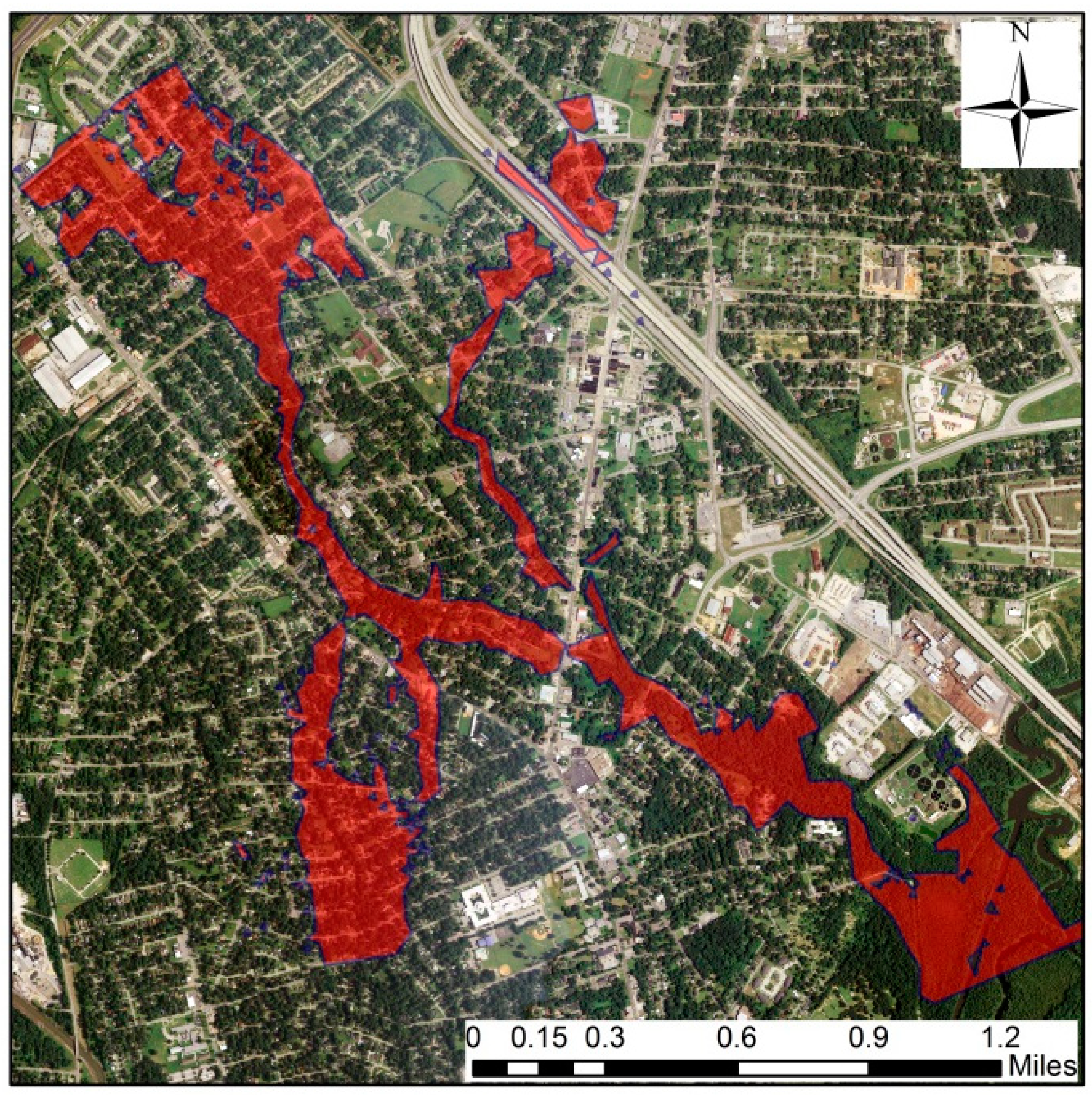
To determine the flood risk based on the floodplain extent and the inundated region boundaries, the river floodplain was simulated using the Hydrologic Engineering Center’s River Analysis System (HEC-RAS 5.0). This software is used as a hydraulic routing model to analyze the river in both steady and unsteady states to obtain the floodplain boundaries, peak discharge, and average depth for each cross-section. Using HEC-GEORAS [51] and ArcGIS extension specifically designed to process geospatial data for use with the HEC-RAS, the river cross-sections were imported to the HEC-RAS 5.0, and the streamflow predictions from SWMM were transferred to the HEC-RAS model. HEC-RAS was run at steady state using the peak flows obtained from SWMM for various return period storms, including 10, 50, and 100 yrs.

2.8. Flood Generating Areas

Kalin and Hantush (2009) [52] developed an index-based, watershed model-driven approach that can assist in identifying sensitive areas in a watershed that could have larger or fewer impacts on low or high flows at a given specific location. The method is based on ranking different parts of a watershed-based on their relative impacts on watershed responses such as peak flow and flooding to anticipate land developments. A similar approach was followed in this study. Two types of indices were used to explore the flood-generating areas in this study. For this, each subwatershed was first disconnected from the watershed to determine their relative contributions to the peak flow (see also [53]). This way, one can identify the subwatersheds that have the highest contribution to downstream flow, and management efforts (such as LIDs) can concentrate on those areas. The first index does not consider the size of the subwatersheds.

$${\alpha }_j=(Q-Q_j)/Q$$

(1)

where $Q$ is flow observed at the outlet when all subwatersheds contribute, and $Q_j$ is flow when all the subwatersheds except subwatershed j contribute to flow.

The second index compensates for the area of each subwatershed.

$${\beta }_j={\alpha }_j/\left({\displaystyle \frac{A_j}{A}}\right)$$

(2)

where $A$: watershed area and $A_j$: subwatershed (j) area.

Both indices might be useful under different situations [52,54]. The first index can be used if flows can be reduced at the outlet of a subwatershed, such as by using a detention pond. The second is more useful if multiple LIDs are needed that are spread over the subwatershed, such as many rain gardens, rain barrels, etc.

3. Results and Discussion

3.1. Performance of the Calibrated Model in Predicting Water Depths

The model was manually calibrated for water depth that was measured at 15 min intervals during 2014–2015.

Table 3. Calibrated SWMM parameters.

Subwatersheds	S (%)	W (%)	Nimp	Nper	n	Dm (cm)	Dp (cm)	Ψ (cm)	K (cm/h)
1, 2, 5, 6, 7, 9, 10	+15	+10	0.01	0.15		0.38	0.25	10.99	0.254
3, 4, 8, 11, 12, 13, 14, 15, 16, 17, 18, 19, 20, 21, 22, 23, 24, 25, 26, 27, 28, 29, 30, 31, 32, 33, 34, 35, 36	−15	−10				0.38	0.25	10.99	0.254
Conduits
16 and 17					0.013
9, 10, 11, 12					0.040
1, 2, 3, 4, 5, 6, 7, 8, 13, 14, 15, 18, 19, 20, 21, 22					0.011

shows the calibrated SWMM parameters. Figure 4 shows the simulated and observed water depth exceedance curves at sites 1–5. The exceedance curves were limited to the top 5% because the focus of this paper is high flows. In general, the simulated water depths match well with the observed water depths. The model underestimated very large depths at three sites. The performance of the model was also assessed by plotting simulated versus observed maximum water depth values from each significant rain event (depth > 12.7 mm, i.e., 0.5 inches) for all sites (Figure 5). Figures show depth estimates based on running SWMM both with rain gauge data and radar-based precipitation estimates. As can be seen from the figures, both rain gauge and radar produced good results for low- to medium-level events. There is no clear evidence of one data source being superior to the other.

Table 4. The values of coefficient of determination R², Nash–Sutcliffe efficiency (NSE), and percent bias (PBIAS) for the calibration events for each site.

Sites	R2			NSE			PBIAS (%)
	Rain Gauge	Radar	Best *	Rain Gauge	Radar	Best *	Rain Gauge	Radar	Best *
1	0.91	0.86	0.93	0.83	0.78	0.88	−12	−16	−11
2	0.93	0.87	0.96	0.87	0.83	0.92	6	2	4
3	0.88	0.85	0.97	0.70	0.69	0.82	17	13	11
4	0.86	0.82	0.95	0.82	0.79	0.92	9	6	6
5	0.90	0.76	0.93	0.86	0.73	0.88	5	8	4

Note(s): * Calculated by picking the predicted flow (radar and rain gauge simulated) leading to smaller residual error on each day. Thus, it is a mixture of rain gauge and radar.

shows the coefficient of determination (R²), Nash–Sutcliffe efficiency (NSE), and percent Bias (PBIAS) values for the calibration events at each site based on the maximum water depth of each storm.

3.2. Flooding Potential of Junctions under Different Design Storms

Based on the estimated time of concentration, a 2 h storm duration was selected for selecting design storms. Rainfall depths corresponding to different return periods were obtained from the National Oceanic and Atmospheric Administration (NOAA) Precipitation Frequency Data Server http://hdsc.nws.noaa.gov/hdsc/pfds (accessed 15 January 2016) For each design storm, rainfall hyetographs were generated using the SCS Type-3 synthetic rainfall distributions [50].

After estimating the design storm intensity and the rainfall hyetograph, the calibrated SWMM model was run to identify areas sensitive to flooding using design storms with 1, 2, 5, 10, 50, and 100-year return periods. None of the junctions overflowed when the return period was 2 years or less, which means urban flooding should not be expected with storms having return periods below 2 years.

Table 5. Overflowing junctions and the duration of overflows for 5, 10, 50, and 100 yr return period storms. Design storm duration is 2 h in each, which is roughly equal to the time of concentration of the TSBW. There is no overflow for 1 or 2 yr return period storms.

Junction (Hours Flooded)	5 Year (P = 3.56”)	10 Year (P = 4.1”)	50 Year (P = 5.54”)	100 Year (P = 6.21”)
J2	X	X	0.35	0.46
J3	X	X	0.24	0.34
J6	X	X	0.28	0.38
J10	X	X	X	0.09
J11	0.3	0.44	0.82	0.98
J13	X	0.21	0.57	0.69
J16	0.23	0.34	0.63	0.76
J19	X	X	0.23	0.31
J20	0.21	0.4	0.84	1.12
J26	X	0.3	0.66	0.81
J28	0.35	0.47	0.73	0.82

summarizes the duration of the inundation of each junction under different return period storms. Note that J20 and J28 are among the most flood-prone sites for all return periods. Both junctions are always in the top three among the flooded junctions.

3.3. Floodplain Maps

The HEC-RAS-generated 100 yr floodplain map is shown in Figure 6 as an example. Based on the extent of the floodplain map, there are four major flood-prone areas. The southeast section on the map is mostly wetlands. Thus, there is no need for mitigation efforts there. The northwest part of the TSBW also appears highly flood prone. Interstate 65 is just upstream of this area with a large intersection, which has a complex drainage network with underground drains. Therefore, this part of TSBW was not considered for either LID practices. The two junctions identified for further analysis earlier, i.e., J20 and J28, are located in the southwest and northeast flood-prone sections shown in Figure 7. The 5-, 10-, and 50-year floodplain maps identified the same areas as flood-prone ones, but to a lesser extent. Therefore, the flood-generating area indices were calculated for junctions 20 and 28 only.

3.4. Flood Generating Areas Index

The flood-generating areas were studied under a 5-yr storm, which is a more frequent event than a 100-yr storm, and thus can be a cause of complaints. As mentioned earlier, smaller return period storms did not lead to junction overflows (Table 5). The two indices defined earlier were used to explore the areas for their potential to cause flooding at junctions 20 and 28. Since there is only one subwatershed draining into junction 28, subwatershed 36 was selected for further study. Junction 20 receives water from subwatersheds 31, 33, 34, and 35. Based on the first index, subwatershed 35 was selected, and subwatershed 34 was considered based on the second index for further analysis. The calculated indices for junction 20 are shown in Figure 7.

Based on the flood generated area index for junction 20, subwatershed 34 has the highest per unit area contributions to the peak flow at junction 20. However, if management efforts (LIDs) are concentrated on subwatershed 34, the flooding at subwatershed 35 would not be considered since part of the subwatershed becomes inundated based on the 5 yr return period floodplain map, and the subwatershed was the flood-generating area based on the calculation of the first index. Therefore, mitigation efforts (low-impact development practices) were concentrated at subcatchments 34, 35, and 36.

3.5. SWMM LID Scenarios

As a first step, the number of buildings were identified in subwatersheds 34, 35, and 36 using the Prichard city map obtained from the city of Mobile’s GIS department (https://cityofmobile.maps.arcgis.com/apps/webappviewer/index.html?id=44b3d1ecf57d4daa919a1e40ecca0c02) (accessed on 23 August 2024). Once the buildings were identified, randomly 20 houses were picked within each subwatershed and the roof area of each building was calculated. After discussing the feasible options with MBNEP, 757-L (200-gallon) rain barrels were considered in half of the houses and 5678-L (1500-gallon) cisterns were considered for the rest of the buildings at all three subwatersheds.

Table 6. Summary of LID selection within subwatersheds 34, 35, and 36.

	Subwatershed #
	# 34	# 35	# 36
Total Buildings	170	440	434
Percentage of Building Area	19%	15.4%	9.3%
Average Roof Area (m2)	153.6	159.1	154.4
Number of Rain Barrels (200 gal) simulated	85	220	217
Number of Cisterns (1500) simulated	85	220	217

summarizes the results. Two 100-gallon RBs and one 1500-gallon cistern were selected because of the common practice and after discussion with MBNEP to capture roughly 25 mm (~1 inch) rainfall falling on roofs in those selected watersheds.

Possible parking areas were identified, and their areas were calculated using the city map of Prichard obtained from the city of Mobile’s GIS department. In subwatershed 35, parking lots occupied 0.9% of the total subwatershed area. In subwatershed 36, they occupied 1.2% of the total subwatershed area. There was no potential parking lot area for the use of permeable pavements in subwatershed 34; therefore, permeable pavements were not considered as an LID option in this subwatershed.

Figure 8 shows the reduction in peak flow, maximum depth, and runoff volume at junction 20 based on LID practices implemented at subwatershed 34, with rain barrels and cisterns as the only LID options. LID practices under different year return periods can reduce peak flow by about 4–7%, depth by nearly 2–5%, and runoff volume by approximately 1–3%.

Figure 9 shows the reduction in peak flow, runoff volume, and maximum water depth at junction 20 under various LID options at subwatershed 35. LID controls under different return periods can decrease peak flow at junction 20 by roughly 18–23%, depth by about 5–15%, and runoff volume by nearly 4–10%. The use of permeable pavements as LIDs did not have much impact, likely due to their small coverage area. As can be seen from the tables, the effectiveness of LID practices is reduced with an increasing return period.

Figure 10A shows the peak flow rates under varying return period events with no LID and with rain barrel as the only LID. Because permeable pavements had a minimal impact (Table 6), it was not considered here. The benefit of using rain barrels is clear from the figure. For instance, a 20-yr maximum flow based on the current conditions (~14.5 m³/s) can be expected to become a 46 yr storm once the suggested rain barrels are installed. Similarly, the bankfull stage flow (~9 m³/s) that is expected to happen on average every 2–3 years could become a ~7-year event after the use of rain barrels as LIDs.

Figure 11 shows the reduction in peak flow, depth, and volume under various LID options at junction 28, which receives all the runoff from subwatershed 36. Based on the table, LID controls under different year return periods can decrease peak flow by approximately 20–25%, depth by 11–15%, and runoff volume by nearly 14–24%. As can be seen from the table, the effectiveness of LID controls is again reduced with an increasing return period.

Figure 10B shows the peak flow rates at junction 28 under varying return period storms with no LID and with rain barrel as the only LID. Because permeable pavements have minimal impact, it was not considered. The benefits of using rain barrels are clear from the figure. For instance, a 20-yr maximum flow based on the current conditions (~14 m³/s) can be expected to become a 44 yr storm once the suggested rain barrels are installed and properly utilized by the residents. Similarly, the use of rain barrels as LIDs can convert the bankfull stage flow at this site (~9.4 m³/s) into a 9-yr event, which is currently expected to happen on average every 4 years.

4. Discussion

The approach presented in this study can easily be replicated in other small cities and communities around the world to address nuisance flooding. The four-step methodology starts with having a reliable urban hydrology and hydraulics model that can handle various LIDs. Having many LID options in the model is critical because the selection of the LIDs depends on cost and feasibility, and the selection processes should be consulted with local authorities and stakeholders. The model, even if it is a physically based one, should be calibrated with monitored streamflow or water depth data. We used water depth in this study because of the challenges in generating reliable stage-discharge curves. If data are not available, we highly recommend collecting some data to calibrate the model. In this research, we collected water level data at five locations with a small budget. The calibrated model can then be used to first identify areas prone to flooding, and then identify key upstream areas that have the highest contribution to flood-prone areas. To achieve the latter, we used two indices proposed by Kalin and Hantush (2009) [52]. Those areas were then considered as potential LID installation sites. Suitable LIDs were identified by consultation with the stakeholders based on cost and feasibility. Once the LIDs and the locations where they will be implemented are identified, the model can be used to assess the potential of the LIDs for flood mitigation.

USEPA’s SWMM model was used in this study to implement this methodology and develop LID-based flood mitigation strategies in Prichard, Alabama. As credited to the British statistician George E. P. Box, “all models are wrong, but some are useful”. The core of this principle is that because models are simplifications of realities, uncertainties are inherent. When interpreting the results, one should keep in mind the uncertainties stemming from the model structure and parameters, and should carefully convey these to the decision makers, which is not an easy task. The results presented and the conclusions reached are tailored to design characteristics of the selected LIDs. The use of larger/smaller rain barrels/cisterns and variation in impervious areas (size and location) within the watershed where they capture runoff could make a large difference in their flood mitigation potential. The same is the case for permeable pavements. We followed the Low Impact Development Handbook for the State of Alabama [39] in selecting the design characteristics. Any differences in the pavement, soil, storage and drainage characteristics of the permeable layer would impact the reduction in peak flow and runoff volume.

Model forcings (e.g., climate data) have errors and uncertainties too, and should also be kept in mind. Conditions of the waterways and many other features of the watershed are often not well known and contribute to the uncertainties in the results. Below are a few key relevant issues pertinent to other uncertainties in this study.

4.1. Uncertainty in Rainfall Data

The simulations in this research were conducted by a model calibrated using field data. Uncertainties associated with such data can impact the model results. Two such sources are of particular interest: precipitation data and stage data. To assess potential uncertainties stemming from precipitation data, rainfall data from radar-based estimates were compared to our rain gauge data for two big events (16–17 May 2015) and are shown in Figure 12. As can be seen, although the patterns of the rainfall time series perfectly match between the two, there are differences in rainfall intensity, and there is no consistent over/under prediction when the two are compared. In the first event, the rain gauge estimates much higher rainfall, but in the second storm, radar estimates are higher. Please note that the radar data used in this study were NEXRAD stage-3, which combines rainfall estimates from several radar stations and further improves them with ground-based precipitation measurements [55]. For several reasons, radar and rain gauge quantitative measurements of precipitation can be different. The science and technology used by rain gauge and radar are highly different. However, the biggest difference is the fact that a rain gauge makes measurements at point-scale, while radar provides areal average estimates (resolution was 4 km in our case). The rain gauge observations are affected by errors due to different causes, like internal frictions and occasional imperfections of the rain gauge, reading errors, the presence of wind, trees or buildings that distort the rain gauge measures, as well as any small debris. Radar measurements can be affected by several sources of error, such as distance of the radar, obstructions, algorithm used in converting reflectivity to rainfall intensity, etc. [56].

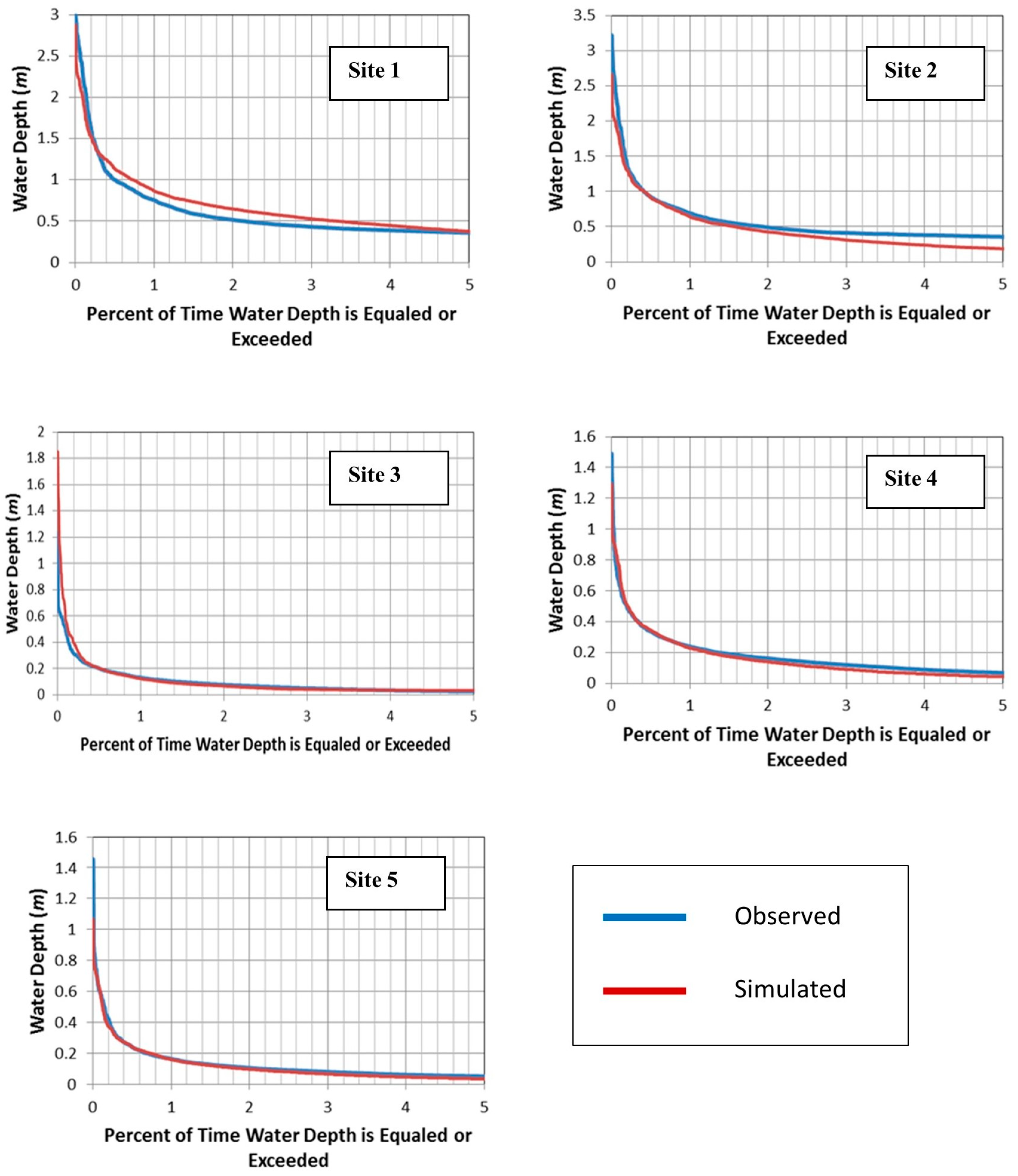
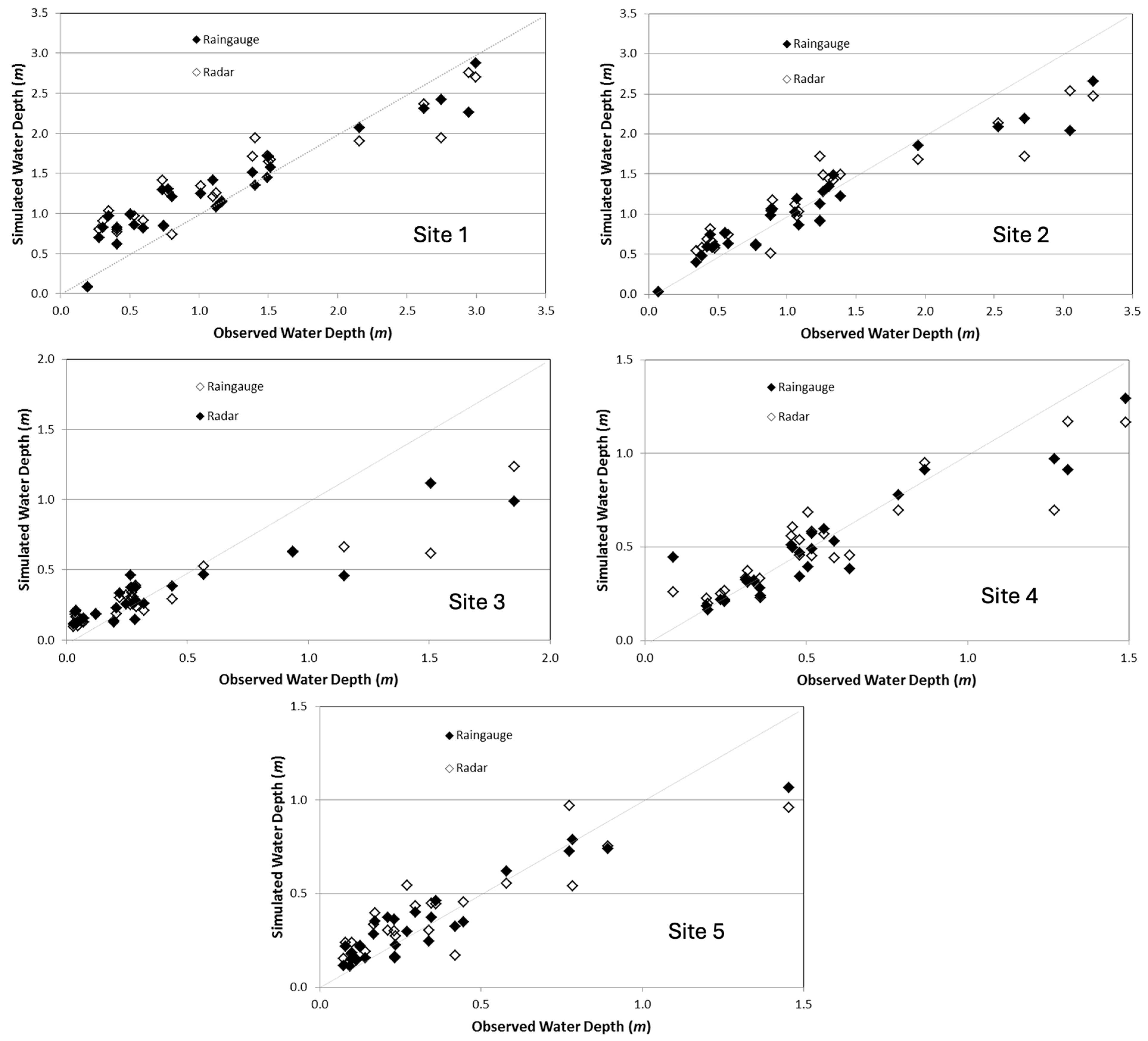
During the rain event on 16 May 2015, the simulated water depth based on the rain gauge rainfall data was greater than the simulated water depth based on the radar-based precipitation data. The trend was the opposite of the rain event on 17 May 2015. Clearly, it is better to consider multiple sources of climate data and present the simulation results with their uncertainties. However, even if we consider the two precipitation data sources, the model still underestimated depths in large events (see Figure 5). The stormwater drainage system of TSBW was not considered in this study because of a lack of information. Stormwater systems can create shortcuts and bypass flows. The watershed boundary also may not be truly reflected when stormwater drains are present. During the study period, there was almost no water at some sites unless there was a large rain event. Many times, although there was some water flowing at sites 4 and 5 during rainless periods, no water was seen at site 3, which is downstream of sites 4 and 5. Therefore, it is highly likely that water leaked to the ground from the concrete channels at some locations, potentially showing up again in channels somewhere else.

4.2. Clogged Channels

During field visits, waterways clogged by debris were observed at multiple sites. This clogging can cause water to back up, leading to local flooding of some roads and the backyards of houses (Figure 13). The Storm Water Management Model (SWMM) cannot account for clogged channel conditions since this situation is unpredictable, and SWMM does not include trash deposits in channels as a model process (again, highly unpredictable).

4.3. Junction 20 and 28 Capacity

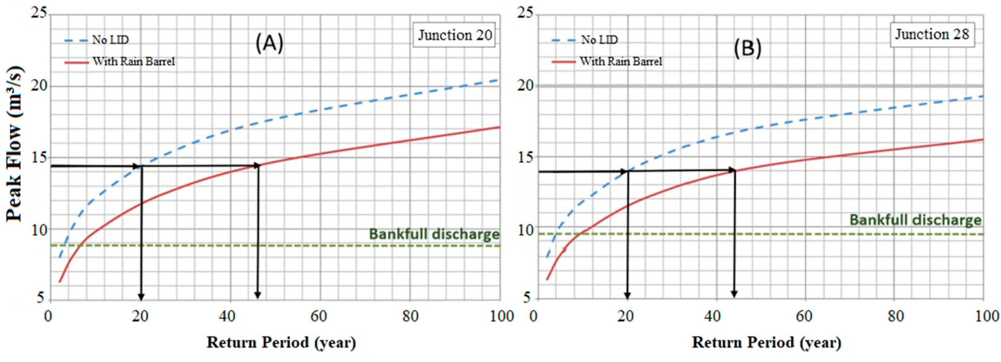
J20 and J28 are the most problematic junctions in the system based on the analysis presented. The problem with junction 28 is its low surcharge depth and low maximum depth in comparison to other junctions in the system. The suggestion for improving the capacity of these junctions is to change their surcharge depth and maximum depth to a higher value. This can be undertaken by changing their physical structure or lowering the level of the storage even though LID principles promote storing and reducing the runoff.

4.4. Outreach and Public Education

One of the most effective ways of mitigating the flooding issue in urban areas and protecting sensitive areas is through outreach and public education. It is important to inform property owners and residents of flooding risks. Channels clogged by vegetation and trash can cause water to back up, leading to some local flooding issues in the TSBW. During field visits, car tires and house items were also observed along the stream (see Figure 13). The mitigating efforts for flooding, in this case, can be easily carried out if locals dispose of the trash properly instead of throwing them into the stream.

5. Summary and Conclusions

Historically, large flows in urban areas have been managed by traditional stormwater management through the use of detention ponds. Low-impact development (LID) is suggested as the solution to problems associated with conventional stormwater management. LID is a land planning and stormwater management technique that minimizes stormwater runoff through natural resource-based site design and seeks to control runoff as near to the source of stormwater as possible. This study provided a framework that follows a systematic approach to address nuisance flooding issues in small cities and communities. The steps are as follows:

• Identify areas prone to flooding. This can be done through modeling or local knowledge.
• Identify areas that have a disproportionately higher contribution to flood risks at areas identified in #1. We use two indices from the literature to achieve this.
• Talk to stakeholders to identify feasible LID options and the potential locations within areas identified in #2.
• Evaluate potential reductions in peaks flows and flows due to the implementation of the LIDs in #3.
• Communicate the findings with the stakeholders and local authorities.

We applied this methodology to investigate the flooding issue at the Toulmins Spring Branch Watershed (TSBW) in coastal Alabama and evaluate various LID options for flood mitigation. The major findings were as follows.

i. Although the study period was a wet period, no widespread flooding was observed based on water stage data collected at five different locations. Flood-related complaints appear to be highly local and potentially linked to lack of maintenance of the drainage system and waterways.

ii. The SWMM model performed well at the TSBW in predicting water levels despite the lack of knowledge of the stormwater drainage system. Neither the city nor the county had a map of the stormwater drainage system. The infrastructure looked very old. Thus, how well the drainage system functions is unknown.

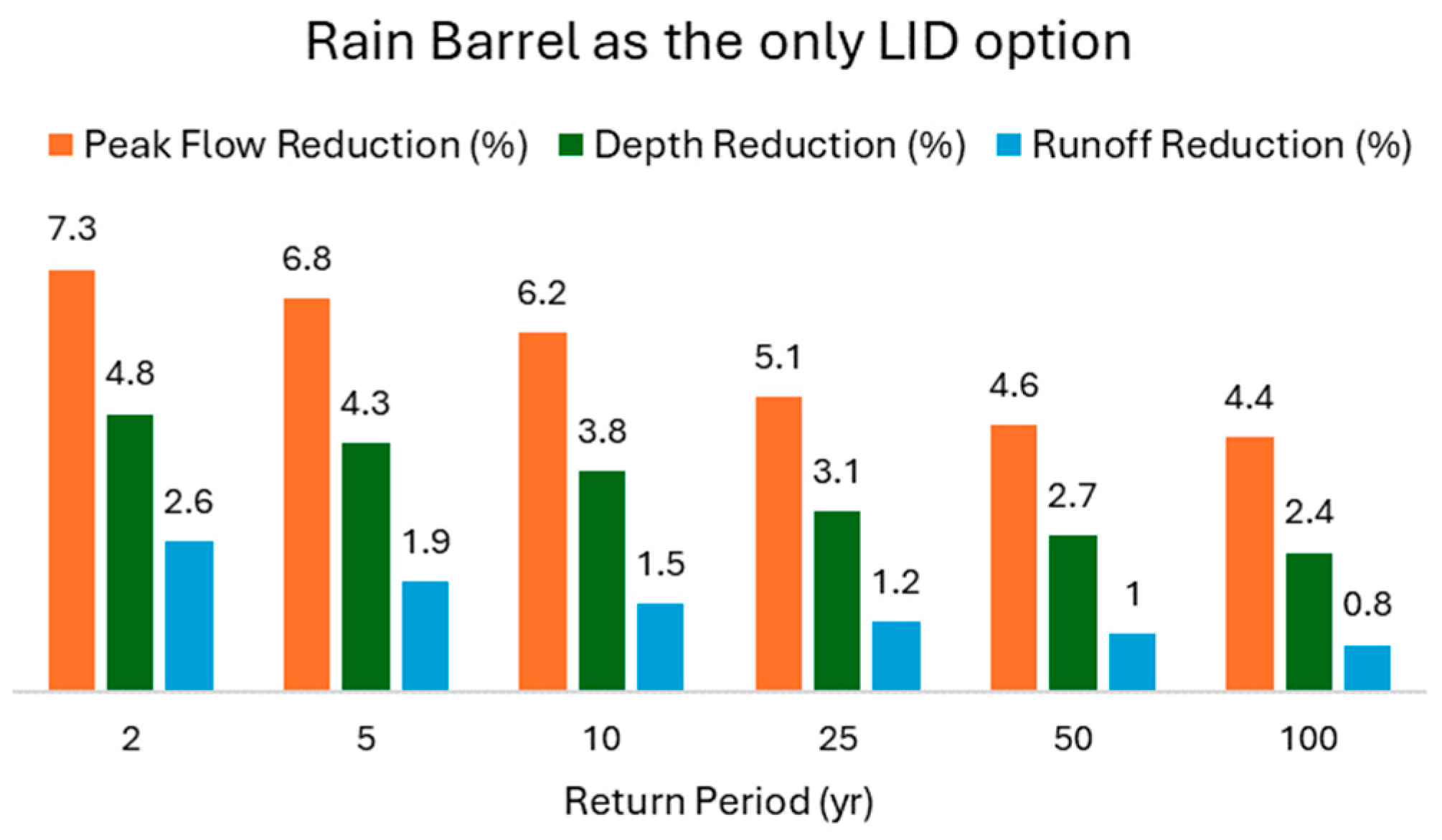
iii. Among various LID options, rain barrels and cisterns were identified as the best choice for this area based on cost and feasibility. Model results show them to be highly effective in reducing peak flows and runoff. Further, they occupy very small areas and require very little maintenance.

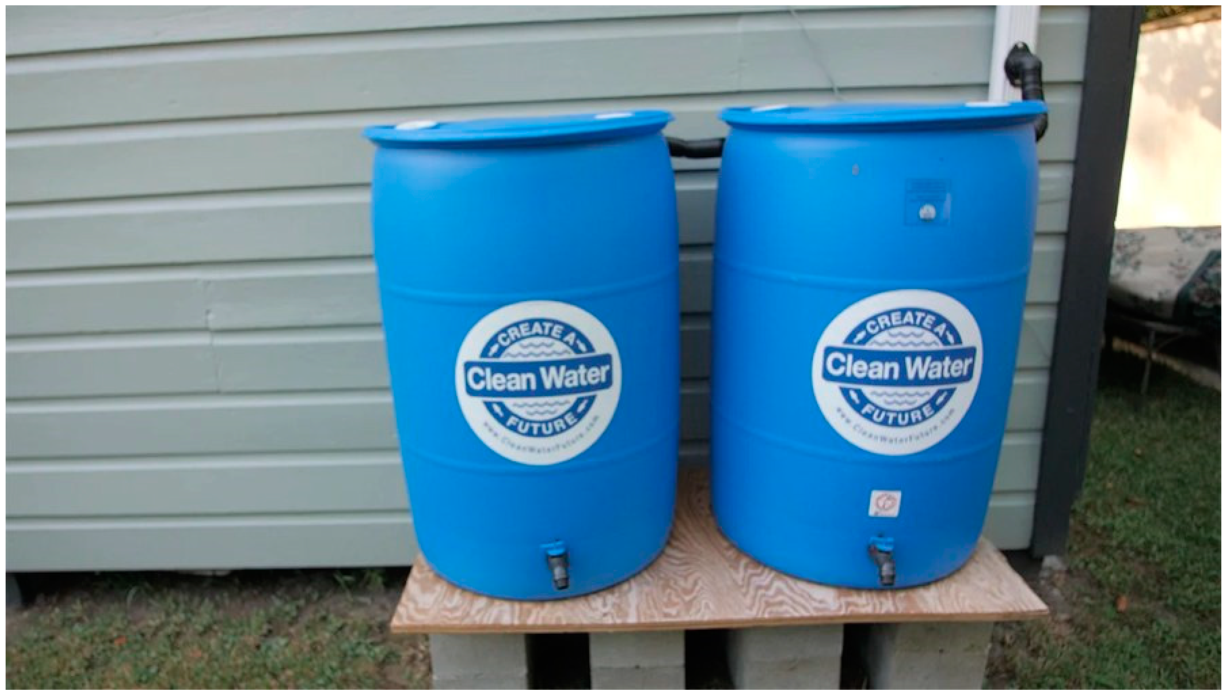
iv. Results were shared with MBNEP, and as of 2021, more than 200 rain barrels have been installed in over 50 homes on the Prichard community website: https://www.mobilebaynep.com/, as shown in Figure 14.

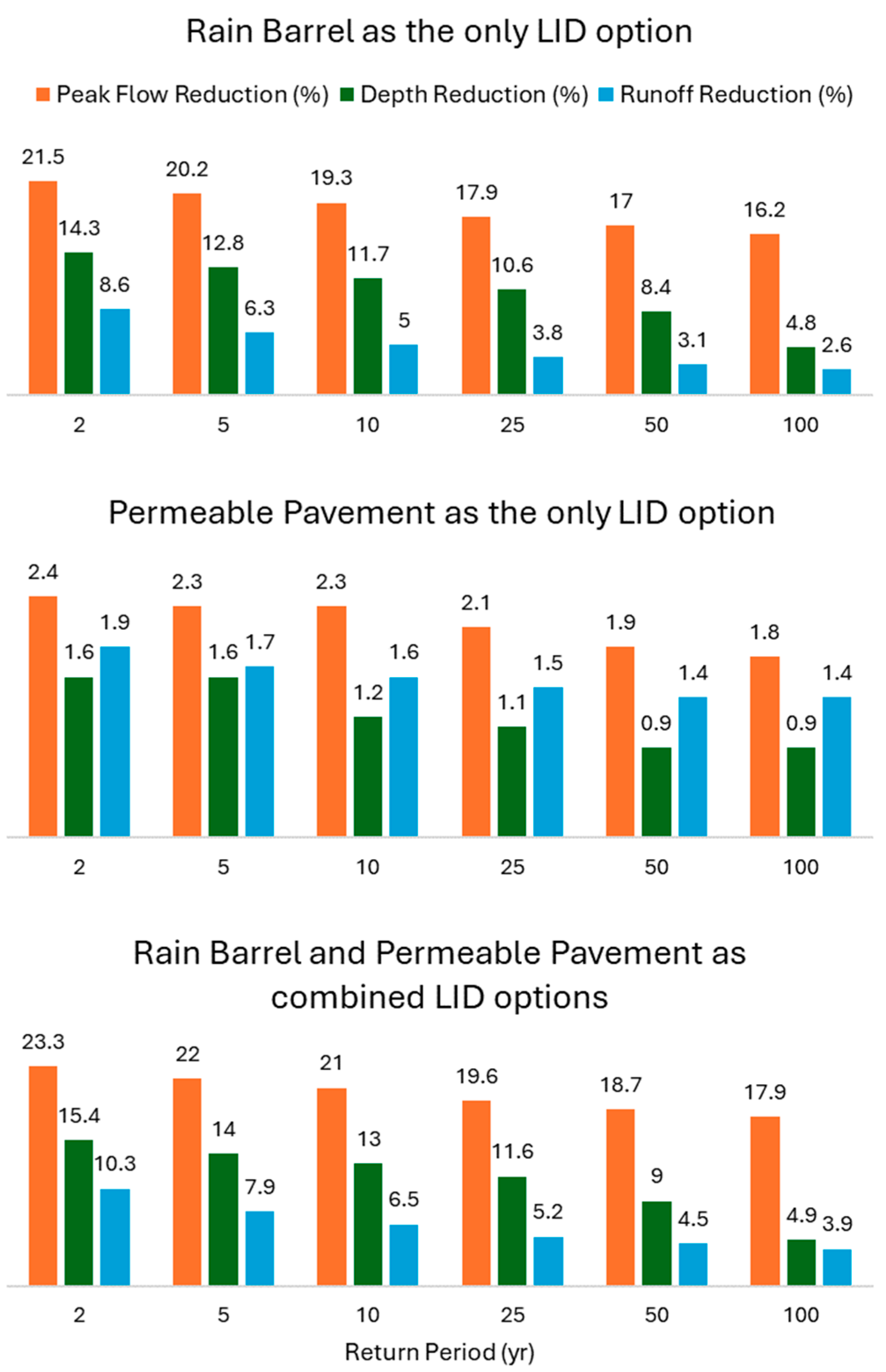
Rain barrels and permeable pavements were simulated as LID practices in TSBW. It was estimated that suggested LID practices, under rainfalls corresponding to return periods of 2, 5, 10, 25, 50, and 100-year storms, can decrease peak flow by 18–25%, depth by 5–16%, and runoff volume by 1–24% compared to the existing conditions where no LIDs exist. These results show that LIDs are worthy of consideration for urban flood control not only in future development but also in established neighborhoods as a stormwater management planning tool.

The real-world applicability of low-impact development (LID) strategies, such as rain barrels and permeable pavements, becomes evident when considering the balance between upfront investment and the potential reduction in flood-related damages. The installation costs for rain barrels and permeable pavements can be offset by their ability to mitigate peak flows and reduce runoff volumes during storm events. By reducing peak flows by up to 20% (as demonstrated in this study for combined systems like RB + PP), these LID practices can significantly lower the likelihood and intensity of localized flooding. Over time, the cumulative benefits of LIDs can outweigh their initial costs, particularly when maintenance expenses are minimal compared to the recurring costs of flood recovery and repair. Moreover, municipalities often provide financial incentives for LID implementation, such as tax credits, grants, or stormwater utility fee reductions, making them even more cost-effective. As extreme weather events become more frequent due to climate change, proactive investment in LID systems not only addresses current stormwater management needs but also enhances long-term resilience, further reducing the economic and social impacts of future flooding.