Article

Groundwater Level Prediction Using Machine Learning and Geostatistical Interpolation Models

Water Resources & Remote Sensing Laboratory (WRRS), Department of Geology, University of Georgia, 210 Field Street, 306 Geography-Geology Building, Athens, GA 30602, USA
*
Author to whom correspondence should be addressed.
Water 2024, 16(19), 2771; https://doi.org/10.3390/w16192771
Submission received: 13 August 2024 / Revised: 24 September 2024 / Accepted: 24 September 2024 / Published: 29 September 2024

Abstract

:
Given the vulnerability of surface water to the direct impacts of climate change, the accurate prediction of groundwater levels has become increasingly important, particularly for dry regions, offering significant resource management benefits. This study presents the first statewide groundwater level anomaly (GWLA) prediction for Arizona across its two distinct aquifer types—unconsolidated sand and gravel aquifers and rock aquifers. Machine learning (ML) models were combined with empirical Bayesian kriging (EBK) geostatistical interpolation models to predict monthly GWLAs between January 2010 and December 2019. Model evaluations were based on the Nash–Sutcliffe efficiency (NSE) and coefficient of determination (R2) metrics. With average NSE/R2 values of 0.62/0.63 and 0.72/0.76 during the validation and test phases, respectively, our multi-model approach demonstrated satisfactory performance, and the predictive accuracy was much higher for the unconsolidated sand and gravel aquifers. By employing a remote sensing-based approach, our proposed model design can be replicated for similar climates globally, and hydrologically data-sparse and remote areas of the world are not left out.

1. Introduction

Global warming is threatening surface water supply in many parts of the word, particularly in arid regions. In these regions, groundwater, a viable alternative and an important source of freshwater, is often limited [1,2]. Considering that groundwater level (GWL) is an indicator of groundwater availability at any given time, monitoring GWLs provides significant insights into the dynamics of recharge and withdrawals and how they influence the long-term availability of groundwater. In arid regions, this can be challenging due to the inadequate distribution of groundwater wells and the presence of spatial and temporal data gaps in monitoring records [3]. Therefore, accurate and reliable predictive tools are essential for supporting the sustainable management of groundwater in these areas [3].
The relationships between GWL fluctuations and explanatory variables are generally complex and nonlinear [4,5,6,7]. However, machine learning (ML) algorithms can effectively learn these relationships. One of such algorithms is the support vector machine (SVM) for regression purposes (SVR), especially when embedded with the radial basis function (RBF) kernel [5,8]. Another algorithm capable of learning these relationships is random forest (RF) [9], which is the most employed ML technique for GWL predictions [10]. Both SVMs and RF are known to give accurate results [10,11].
Several studies have shown the RBF–SVR model to outperform various other techniques, such as artificial neural network (ANN) [12,13,14], radial basis function neural network (RBF–NN) [15], the autoregressive integrated moving average (ARIMA) model [16], RF [8], and the gradient boosting mechanism (GBM) [8]. These studies also attribute the success of SVMs to their strong prediction capability and the ability to generalize well to unseen data.
Likewise, various studies have reported success using RF for GWL prediction. For example, it outperformed K-nearest neighbor (KNN), ANN, and SVR based on root mean square error (RMSE) values during testing [17]; ANN and SVR based on R-squared (R2), mean absolute error (MAE), and RMSE values in training and R2 and MAE values in testing [11]; multilinear regression (MLR) based on R2, MAE, and RMSE values in both training and testing [18]; decision trees (DTs) and SVRs based on its R2 and RMSE values in testing [19]; and the XGBoost regressor based on its MAE and RMSE values in testing [20].
In addition to traditional ML methods, geostatistical interpolation (GI) techniques are also commonly used for GWL prediction. Kriging is the most utilized GI technique [21,22], where the measured values of a variable (GWL, in this case) at specific locations are used to make predictions at unmeasured areas. It relies on the correlation between the measured values as a function of distance, depicted by a semivariogram, to assign weights that describe the contribution of each measured point to the prediction at unmeasured locations [23]. Kriging presents an important advantage over other interpolation methods in being able to quantify and minimize prediction uncertainties [23].
Classical kriging (CK), the traditional form of kriging, relies on a single semivariogram assumed to be the true representation of the measured data. In contrast, empirical Bayesian kriging (EBK), an advanced kriging approach, incorporates multiple semivariograms to account for the uncertainties associated with estimating a single semivariogram [23]. Thus, EBK is a more robust kriging algorithm [23], and studies such as Bouhout et al. (2022) [24] and Hussain et al. (2016) [25] have demonstrated its superior performance in GWL prediction applications.
Our review of the existing literature suggests that RBF–SVR, RF, and EBK models are some of the most effective GWL prediction tools. To enhance the prediction accuracy, we propose an approach that integrates all three techniques to predict the monthly GWLAs across the state of Arizona (representative of arid/semi-arid systems) between January 2010 and December 2019, using remotely sensed predictor variables.

2. Materials and Methods

Natural groundwater recharge in arid regions is often limited, raising concerns about the sustained availability of freshwater in these regions. Climate change exacerbates these issues by intensifying the hydrologic cycle, resulting in increased evapotranspiration rates and a reduction in the soil moisture available to recharge groundwater systems [26,27]. In a recent study, Zowam et al. (2023) [27] quantified terrestrial water cycle intensity (WCI) changes across the contiguous United States (CONUS) attributable to climate change and showed that the state of Arizona might be experiencing much higher relative WCI rates on average than other arid regions in the CONUS. These factors underscore the need for accurate prediction of the GWL in such regions to continue to effectively manage the potentially limited freshwater resources therein.

2.1. The Study Area and Target Variable

The study area, covering about 114,000 mi2, is located in the southwest U.S. (Figure 1). Its surficial geology is characterized primarily by unconsolidated deposits in the south/southwest–northwest corner of the state, with various rocks dominating the other regions [28]. The consolidated rocks are mainly sedimentary and extrusive igneous (volcanic) rocks and constitute the mountain ranges that border the basins filled with unconsolidated materials [29]. These rocks are the main sources of sedimentary materials that fill the basin and have very low permeability and groundwater flow rates [29]. Many communities depend solely on groundwater to meet their water needs, which has led to a long history of over-extraction in many parts of the state [30]. In the late 1980s, the Colorado river arrived in Arizona and eased some of the pressure on groundwater to meet these needs, but the prolonged drought in the Colorado river basin, coupled with projected warming temperatures, is expected to not only reduce the surface water availability in the state but also further stress the aquifers in the region [30].
Daily GWL data from 59 monitoring wells were downloaded from the National Groundwater Monitoring Network (NGWMN) portal (https://cida.usgs.gov/ngwmn/index.jsp, accessed on 29 January 2023). Among these wells, 38 were drilled into unconsolidated sand and gravel aquifers and are managed by the Arizona Department of Water Resources (ADWR), while the remaining 21 were drilled into consolidated rock aquifers (Figure 1). Three of the rock aquifer wells used in this study are maintained by the U.S. Geological Survey (USGS), and the rest are managed by the ADWR. The depths of these wells varied and ranged from 89 to 1600 feet below ground surface (bgs) for the sand and gravel aquifers, and about 25 to 851 feet bgs for the rock aquifers, and the aquifers were predominantly unconfined. Daily GWL measurements were aggregated into monthly averages from January 2010 to December 2019.
Missing data is the most common challenge in real-world ML applications [31], and various methods exist to address this issue. The simplest of these methods is mean imputation (MI) [31]. In MI, the mean values of available observations are used to fill in missing observations, which has proven to work well with small variance distributions [32,33], i.e., distributions with a coefficient of variation (CV) less than 10% [34]. Therefore, with CV values ranging from 0.01 to 0.91% for the unconsolidated aquifers and 0.001 to 0.21% for the rock aquifers, the MI method was ideal for the target variable (monthly GWL). Missing monthly values were replaced with the annual average GWL for the given year.
To compute monthly GWLA, we calculated the mean GWL at each well and subtracted the monthly measurements from this mean value.

2.2. Predictor Variables

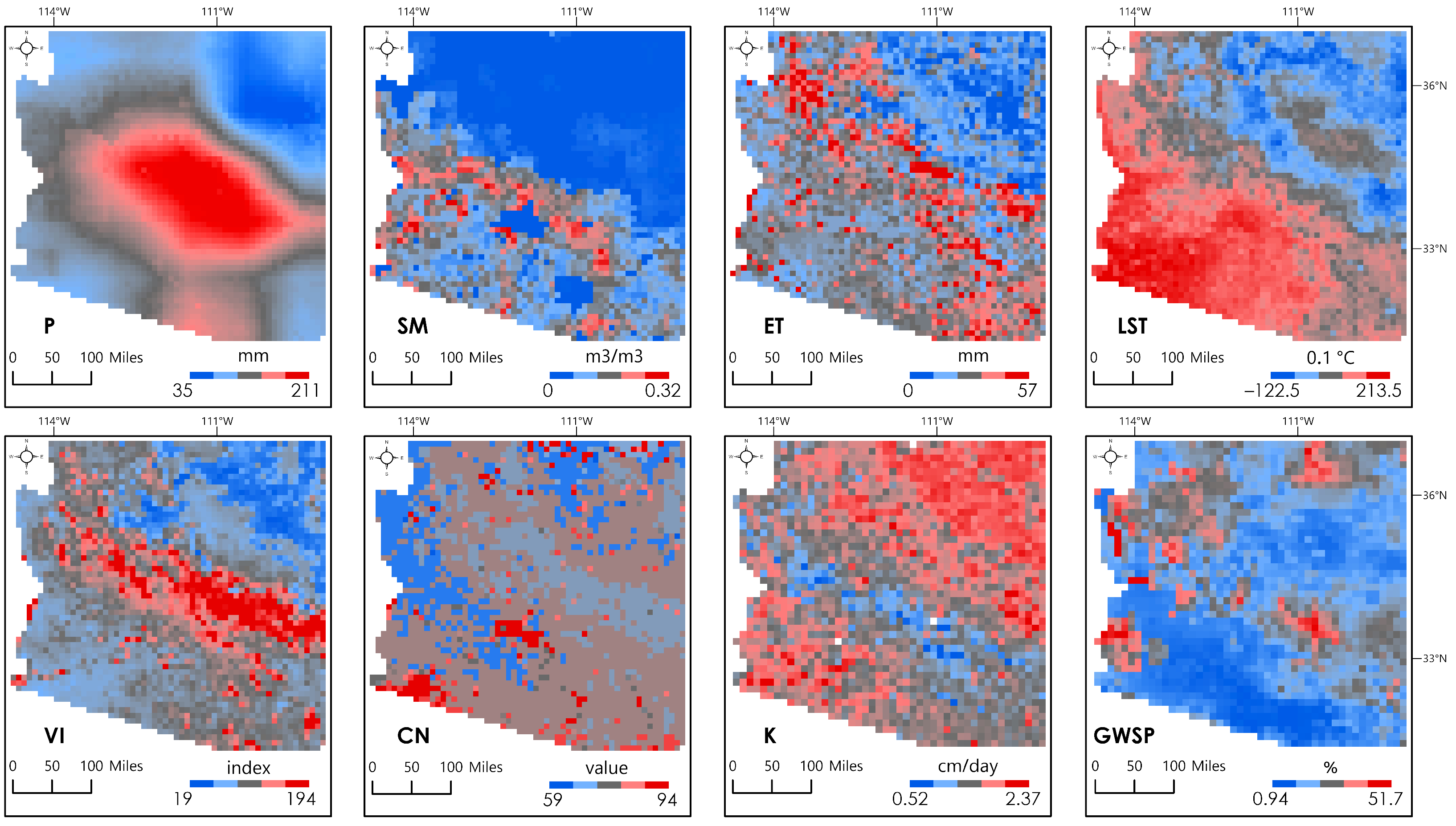
The selection of the input variables was informed by the Seyoum et al. (2019) [35] study as well as established hydrogeological principles. The initial variables included precipitation, soil moisture, evapotranspiration, land surface temperature, vegetation index, curve number, saturated hydraulic conductivity, and groundwater storage anomalies (Figure 2).

2.2.1. Precipitation (P)

Precipitation is the most important hydrological variable for predicting groundwater recharge [36], thus playing a crucial role in determining GWL. In the last two decades, satellite-based precipitation measurement techniques have seen significant advancements, and the Global Precipitation Measurement Mission (GPM) using the Integrated Multi-Satellite Retrievals for the GPM (IMERG) algorithm stands out as one of the best alternatives to ground-based measurements [27,37]. In particular, the GPM mission demonstrates significant potential to mitigate the challenges associated with estimating precipitation in arid regions [38]. In addition, under light rainfall conditions (typical of these regions), IMERG tends to produce lower detection errors and generally more accurate estimates [39]. The final run of the IMERG system provides the most accurate precipitation measurements, making it ideal for research purposes [40]. A monthly IMERG (final run) dataset with a 0.1° × 0.1° grid resolution was downloaded from the National Aeronautics and Space Administration (NASA) data portal for January 2010 to December 2019 (https://gpm.nasa.gov/data/directory, accessed on 11 May 2021).

2.2.2. Soil Moisture (SM)

SM and GWL tend to demonstrate a negative relationship [41,42,43], which can be much stronger for shallow groundwater [41]. For this study, we utilized a research product that integrated measurement efforts from both the European Space Agency (ESA) and NASA (https://doi.org/10.1594/PANGAEA.940409, accessed on 12 February 2023). The dataset was generated by downscaling ESA’s Climate Change Initiative (CCI) data using NASA’s Soil Moisture Active and Passive (SMAP) data [44]. The global dataset had a grid size of 9 km (~0.08° × 0.08°) and a daily temporal resolution covering a 43-year period from 1978 to 2020 [44]. We converted the daily rasters into monthly averages spanning our study period and extracted the monthly data for the study area.

2.2.3. Evapotranspiration (ET)

The combined effects of liquid water losses from soil surfaces (evaporation) and its uptake by plants (transpiration) limit the amount that infiltrates the ground, thereby affecting GWLs. We utilized a global dataset with a fine grid size of 1 km (~0.01° × 0.01°) and a monthly temporal resolution (https://doi.org/10.7910/DVN/ZGOUED, accessed on 3 July 2021). The dataset was obtained by synthesizing the best-performing satellite ET products following validation against flux eddy covariance ET and performed better than local products across the United States, China, and the continent of Africa [45].

2.2.4. Land Surface Temperature (LST)

LST tends to exhibit a positive relationship with GWL, which is more pronounced for shallow groundwater [41]. This study utilized a gap-filled, continuous LST dataset generated by filling in missing pixels in the Moderate-Resolution Imaging Spectroradiometer (MODIS) 1 km resolution LST daily product [46]. Daytime (1:30 PM) and nighttime (1:30 AM) global datasets were downloaded from the Iowa State University research repository (https://doi.org/10.25380/iastate.c.5078492.v3, accessed on 12 February 2023). The downloaded rasters were converted into monthly averages, and the final LST dataset was obtained by averaging the daytime and nighttime monthly estimates.

2.2.5. Vegetation Index (VI)

The presence of vegetation may affect groundwater recharge (and GWLs) in various ways, including slowing down runoff and enhancing ET through transpiration. VI values are unitless and help to visualize the locations and relative abundance of green vegetation. A monthly dataset with a 0.1° × 0.1° grid resolution was accessed and downloaded from the NASA Earth Observations (NEO) data portal (https://neo.gsfc.nasa.gov/view.php?datasetId=MOD_NDVI_M&date=2010-12-01, accessed on 12 February 2023).

2.2.6. Curve Number (CN) and Runoff Depth (R)

CN is a dimensionless parameter that characterizes the runoff potential of a surface. It is influenced by land use, soil characteristics, and the antecedent moisture conditions of soils. Lower numbers typically correspond to permeable soils with high infiltration rates, while higher numbers are associated with impervious surfaces and limited infiltration capacities. The CNs utilized in this study were generated using a 250 m hydrological soil group dataset (HYSOG250m) and the 2015 ESA–CCI 300 m land cover dataset, and available at a 250 m grid resolution (https://doi.org/10.6084/m9.figshare.7756202.v1, accessed on 12 February 2023).
With the CN data, we generated a monthly dataset of R for the period of study using Grove et al. (1998)’s [47] equations:
R = P 0.2 S 2 P + 0.8 S
Given that
S = 1000 C N   10
where R = runoff depth, P = precipitation, S = potential maximum retention, and CN is the curve number [47].

2.2.7. Soil Saturated Hydraulic Conductivity (Ks and PKs)

Soil saturated hydraulic conductivity describes the ability of soils to transmit water under saturated conditions [48]. Using remotely sensed environmental variables and the RF ML technique, Gupta et al. (2021) [49] generated four global Ks maps representing four different soil depths at a 1 km (~0.01° × 0.01°) resolution. All four maps were utilized in this study (https://doi.org/10.5281/zenodo.3935359, accessed on 11 October 2023).
To obtain a continuous and dynamic Ks dataset, we multiplied each Ks value by the monthly precipitation estimates. We selected precipitation as it is a primary driver of water input into the soil and significantly influences Ks. By integrating the precipitation data with Ks, we added temporal variability to the Ks variable, making it suitable for our ML models.
P × K s i = ( P K s ) i
Here, P is the precipitation dataset, Ks is the soil saturated hydraulic conductivity dataset at a depth of i, and i ranges from 1 to 4. The four resulting outputs from Equation (3) were averaged into a single comprehensive PKs dataset for the study area.

2.2.8. Groundwater Storage Percentile (GWSP)

Using terrestrial water storage (TWS) observations from the Gravity Recovery and Climate Experiment (GRACE) satellite mission and a numerical model representing the interactions between water and energy across the Earth’s surface, scientists at NASA are able to determine weekly groundwater conditions, expressed as percentiles, based on comparison with historical data [50]. These percentiles indicate the probability of occurrence within the 1948 to 2014 period of record and are generated at a spatial resolution of 0.125° × 0.125° over North America from April 2002 to the present [50]. We downloaded the monthly averages of the GWSP from the Giovanni data portal (https://giovanni.gsfc.nasa.gov/giovanni/, accessed on 10 October 2023) for our period of study. Considering all the input datasets, the GWSP had the largest spatial resolution (0.125° × 0.125°), requiring all the other datasets to be resampled (upscaled) to the spatial resolution of the GWSP rasters.
Groundwater recharge is typically computed using a simple water balance approach assuming negligible changes in soil water storage in the unsaturated zone [51]. Based on this idea, we introduced a secondary input variable, called the recharge index (RI), to represent the balance between the water inflows and outflows within each 0.125° × 0.125° grid and the amount potentially available to recharge groundwater.
R I = P E T R
where P is precipitation; ET is evapotranspiration; R is runoff depth; and RI is the recharge index for a given grid.
GWLs from monitoring wells located within a grid were assumed to be representative of the entire grid, as were the predictor variables. Ultimately, this study utilized six predictor variables, namely soil moisture (SM), land surface temperature (LST), the vegetation index (VI), saturated hydraulic conductivity (Ks), the groundwater storage percentile (GWSP), and the recharge index (RI) (Table 1).

2.3. Model Algorithms

Developing an acceptable ML model with a monthly temporal resolution requires approximately 10–12 years of data [52]. Here, we utilize 10 years of monthly data (2010–2019), meeting the acceptable sample size threshold. Selecting algorithms or models that are most appropriate for the data is another important aspect of ML. Getting this step wrong could result in unreliable predictions, leading to a disappointing predictive performance and misleading conclusions [53]. In this study, we selected two ML algorithms (and a GI technique) from a pool of candidates. The selected techniques are discussed in detail below:

2.3.1. The SVM and SVR

SVM was introduced by Vladimir Vapnik based on the idea of nonlinear mapping of input vectors to a high-dimensional feature space and constructing an optimal hyperplane to effectively separate the different groups or classes within that space [54]. The generalization capabilities of SVMs led to the development of the less popular SVR for real-value (regression) problems [55].
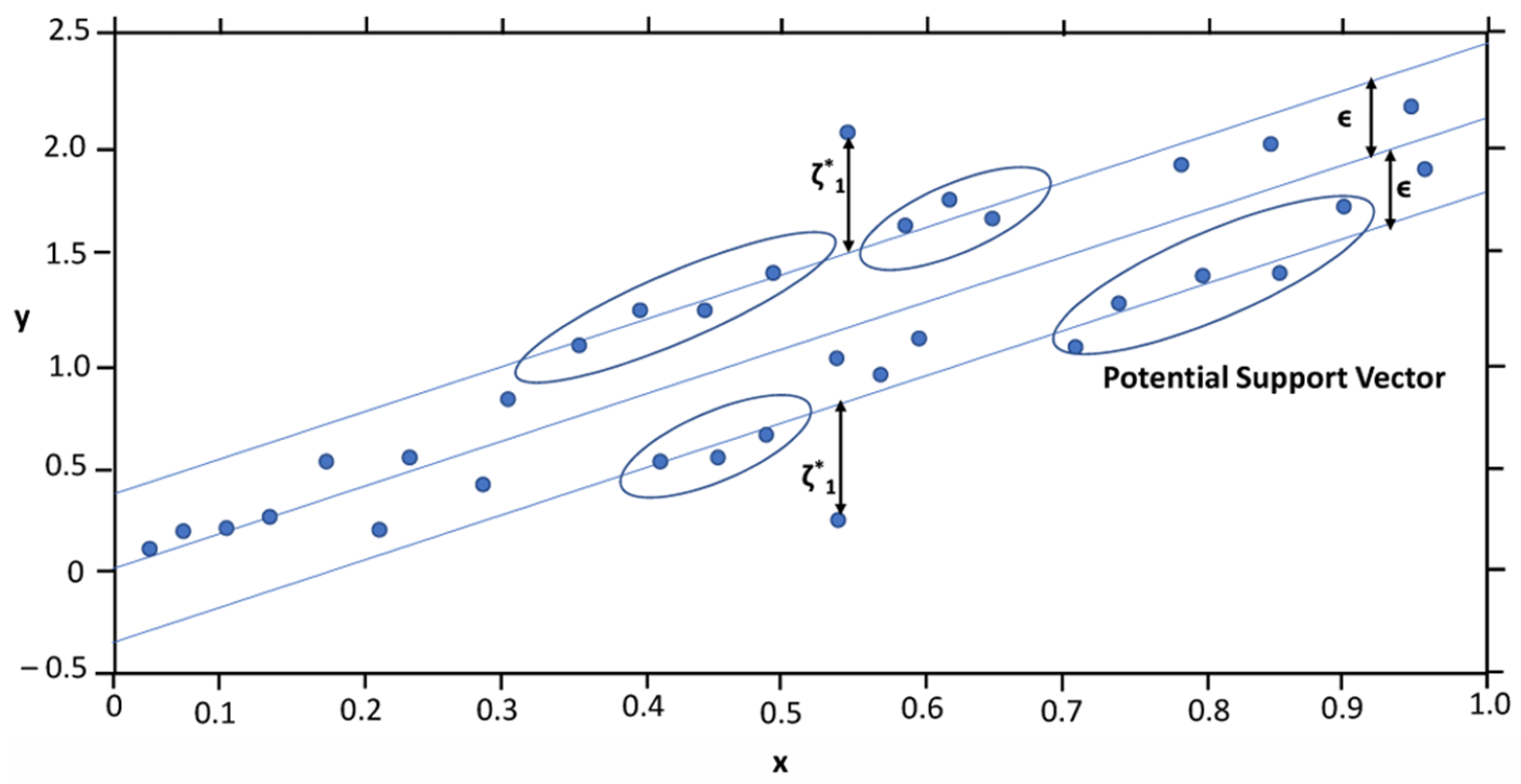
First proposed in 1996 by Harris Drucker and his colleagues [56], the SVR has become an effective tool for prediction problems, demonstrating excellent generalization abilities and a high prediction accuracy [55]. It works by incorporating a loss function (known as the epsilon insensitive margin of error, ϵ) in the form of a flexible tube formed symmetrically above and below the estimated function, where the prediction errors (ζ*) within the tube are accepted and those that fall outside are penalized (Figure 3). The objective of the SVR is to find the narrowest possible tube around the estimated function in a way that minimizes the prediction errors [55,57].
In general, the performance of the SVR model depends on the tube size (epsilon, ϵ), the regularization constant (C), and the choice of kernel function [58,59,60]. The C hyperparameter controls the complexity of the model, where large values may lead to overfitting [58,61]. By overfitting, the model learns the training data well but generalizes poorly, i.e., predicts poorly on new unseen data. Kernel functions are used to transform the data into the higher-dimensional feature space, enabling linear machine learning to improve the representation of the nonlinear relationships that exist in the original input space [62]. While there is no guide to the appropriate kernel functions for specific datasets, the most commonly used are the RBF and polynomial functions [63]. RBFs are versatile kernels used when there is a lack of prior knowledge about the data [64]. Such models (RBF-SVR) require an additional hyperparameter, gamma (γ), in addition to C and ϵ, which controls the width of the RBF [60,65,66]. The C hyperparameter must be a positive number, while ϵ and γ can be positive or zero [66].

2.3.2. RF

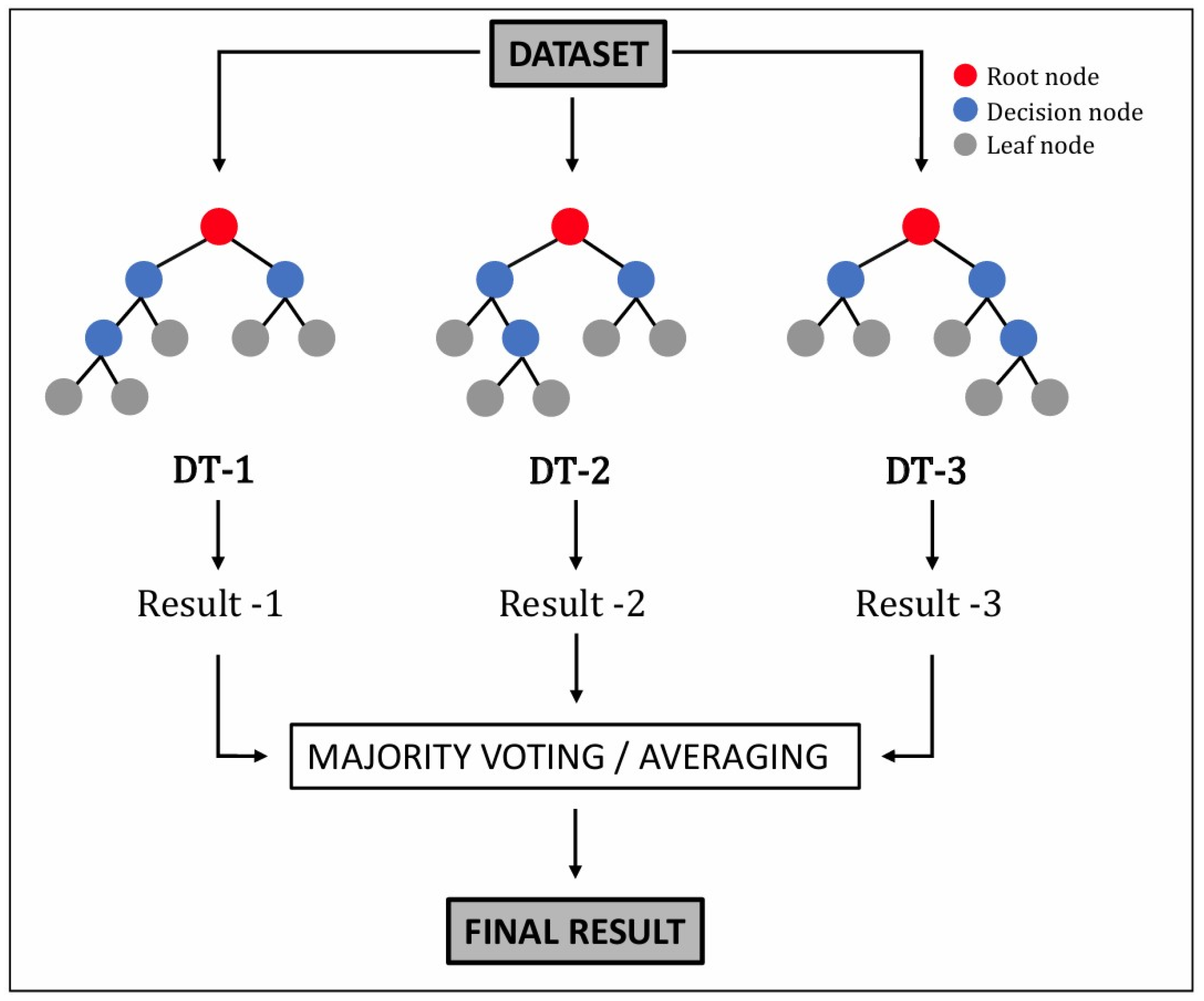
The RF ML algorithm is an ensemble algorithm of multiple trees that improves the prediction accuracies of the single DT algorithm [19,67]. The different DTs are trained with subsets of the input variables and bootstrapped samples of the original training data such that each DT is unique, resulting in reduced variance [11]. By bootstrapping, samples are randomly drawn (with replacement) from the original training data, maintaining the sample size of the training data. Because the sampling is carried out with replacement, a particular observation may appear multiple times in a bootstrapped sample.
Decision points in the DT structure are called nodes. At the nodes, tree branches are created based on the splitting criteria (Figure 4). The first node (without prior branching) is the root [68]. From the root, each node is split using the best variable among the subset of input variables chosen at that node [69]. The leaf is the final node (with no further branching) associated with an output value [68].
RF model hyperparameters are the number of trees (DTs) and the number of input variables in the random subset at each node [11,69]. The final predictions are either determined by majority votes from individual DTs (classification) or by averaging the predictions from all the trees (regression) [69,70].

2.3.3. EBK

EBK differs from CK in the way it optimizes the parameter uncertainty associated with creating a single semivariogram and the way it automates the optimization process. In a single semivariogram, the semivariance (the y-axis) measures the spatial dependency between pairs of observations or samples, and the lag (the x-axis) is their separation distance (Figure 5a). Depending on the characteristics of the data, a semivariogram may display three important components: a sill, a range, and a nugget (Figure 5a). The range is the distance (or lag) beyond which samples are not spatially autocorrelated, and the sill is the semivariance at that distance. The nugget is the y-intercept of the semivariogram and represents variability at distances much smaller than the minimum spacing between pairs of sample points.
With EBK, the input data are divided into subsets, specifying parameters such as the size of the subsets (subset size) and the degree of overlap between them (overlap factor). Within each subset, a semivariogram distribution is produced (Figure 5b), and predictions are made for each location using the distribution from one or more subsets [23].

2.4. Model Design

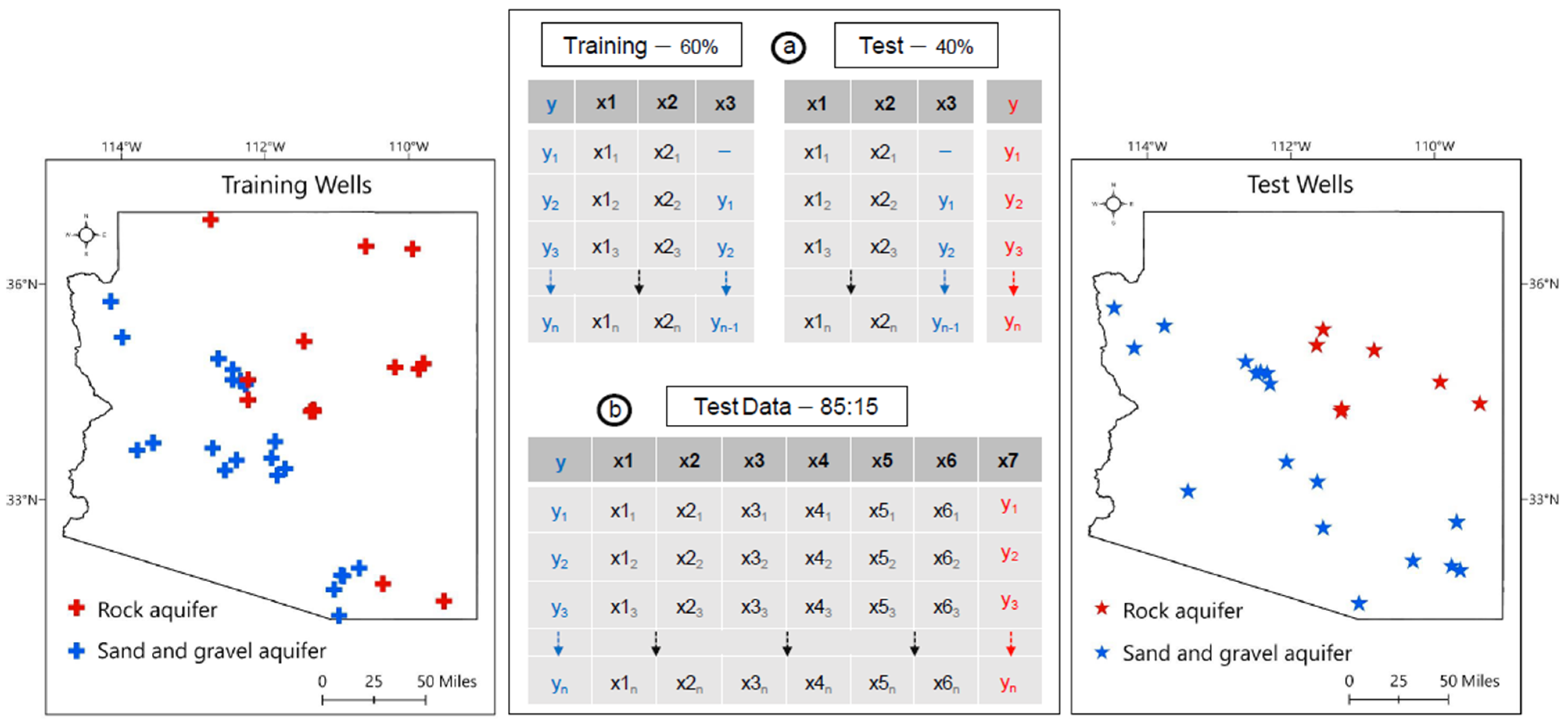
The initial phase of the analysis aimed to assess the feasibility of ML to capture spatiotemporal patterns of GWLAs across the study area. For spatial patterns, we trained 12 different SVR models (each corresponding to a specific month) on sixty percent of the dataset using manually tuned values of γ, C, and ϵ and tested each of the trained models with the remaining forty percent (Figure 6a). Each model was trained using three predictor variables—LST, RI, and the previous month’s GWLA (except for the first month). Incorporating GWL from a prior time step is common practice. It is the most employed type of input data in GWL prediction [52]. To evaluate ML feasibility for temporal patterns, we utilized the same dataset as the test set but used all six predictor variables and the predicted output—replacing the “previous month GWLA” variable to ensure consistency in the number of predictors for each observation (Figure 6b). Following another random train/test split procedure, an RF model was trained on eighty-five percent of the data and tested on the remaining fifteen percent. The models were evaluated for their performance and predictive accuracy using the Nash–Sutcliffe efficiency (NSE) and the coefficient of determination (R2), respectively. The NSE ranges from –∞ to 1, while R2 ranges from 0 to 1. For both metrics, a perfect prediction would yield a value of 1.
Based on the results of the preliminary assessments, it was evident that incorporating some approximation of the GWL as a predictor variable would significantly enhance the model performance and predictive accuracy. Therefore, we sought to use EBK for those approximations. To ensure that the EBK predictions covered the study area, we obtained additional GWL data from 18 nearby monitoring wells outside the study area. A total of 120 EBK models were constructed using the Geostatistical Wizard interpolation tool in ArcGIS PRO, and monthly predictions from those models were converted into anomalies and incorporated into the dataset. A single RF ML model (Figure 7) was then developed to learn the patterns in substantial portions of the augmented dataset.
This approach was first validated at three monitoring well locations. The measurements corresponding to those locations were removed from the dataset before performing the EBK. Because the accuracy of kriging is significantly influenced by the number and density of kriging points, we could not afford to eliminate additional wells (and their corresponding data) from the dataset. Subsequently, the EBK process was repeated using the entire dataset, and a final RF model was trained on a significant portion of this dataset, tested on a smaller subset, and eventually deployed at locations without monitoring wells.

3. Results

The analyses were conducted in RStudio (version 2023.06.0+421) and ArcGIS Pro (version 2.9.3). The results are presented below.

3.1. Initial Assessment of ML Capabilities

The SVR models effectively captured the spatial patterns of GWLA variation across the study area, based on the NSE and R2 values (Table 2). Each monthly model (except for the January model) was trained using the previous month’s GWLA data. The unavailability of previous month measurements as input for the first (January) model resulted in its suboptimal performance. However, the predictions from subsequent models were averaged with the January prediction to obtain the final model predictions. Incorporating the suboptimal performance of the first model with the strengths of the subsequent models reduced model uncertainties and produced more accurate predictions (for the subsequent models).
We observed notably high prediction accuracies for the summer months. In particular, the July model, with an NSE of 0.96 and an R2 of 0.97, demonstrated exceptional performance (Table 2).
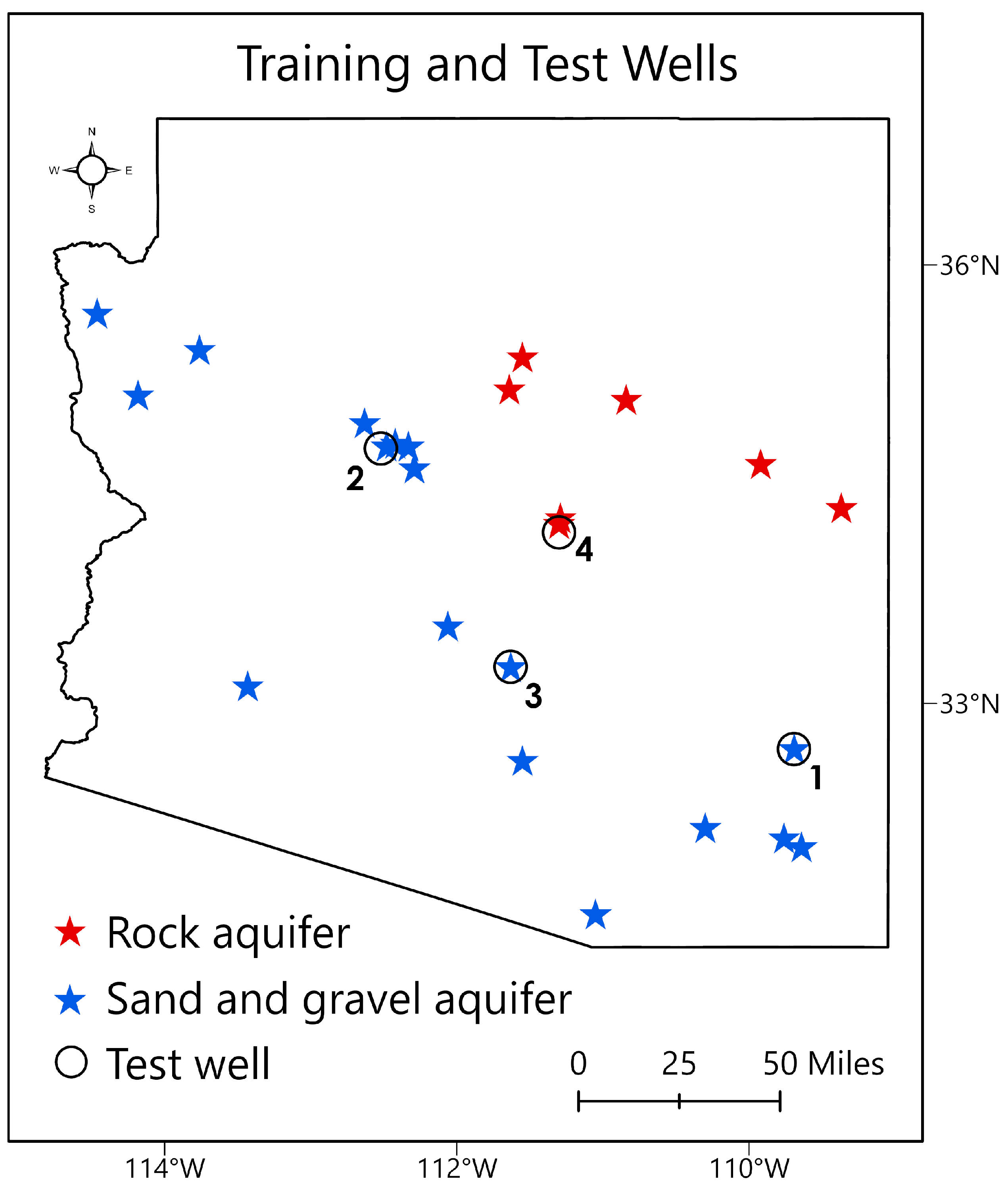
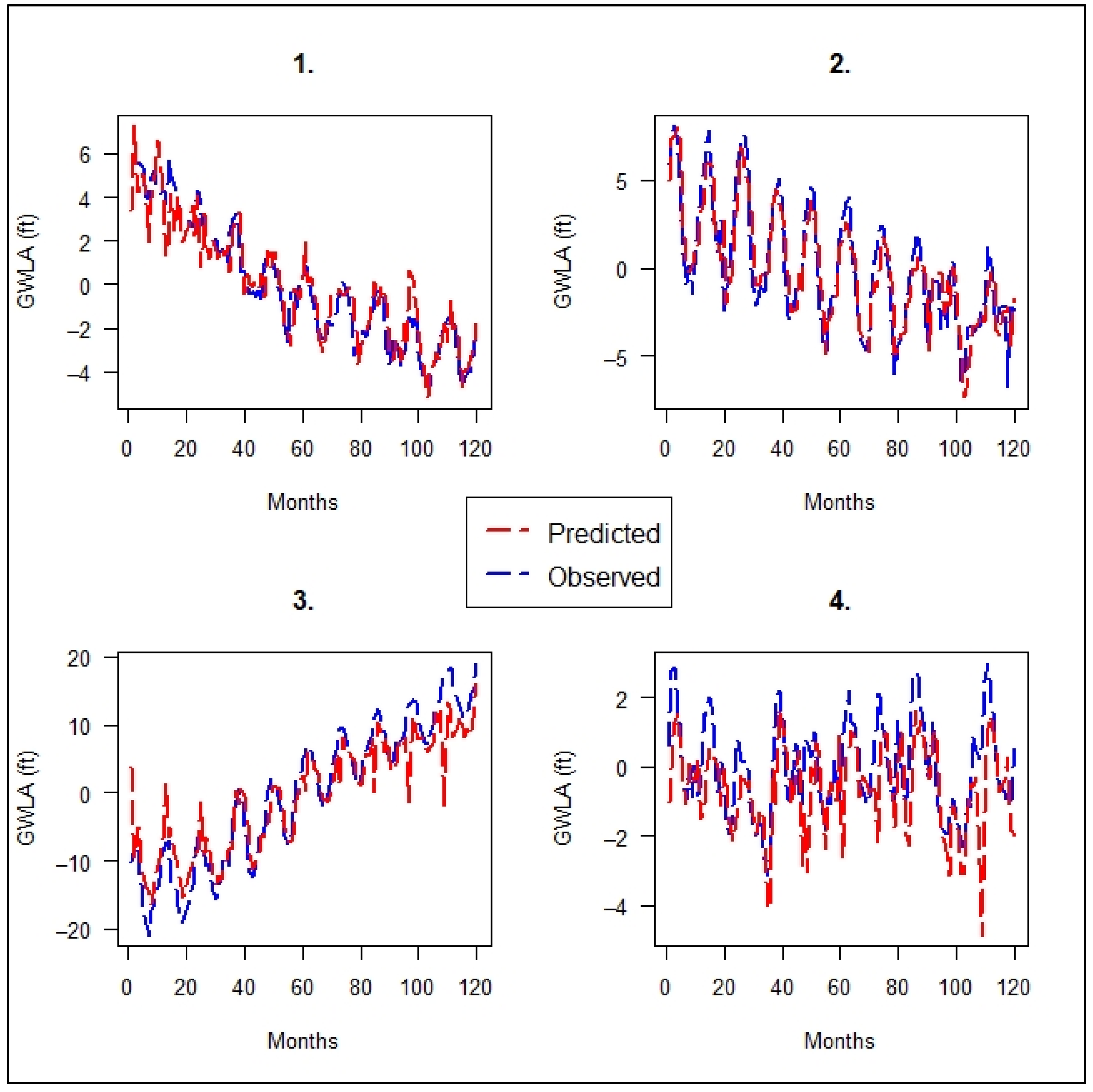
The test set (Figure 6b) was augmented with the predicted output of the SVR models, and a single RF model was trained on eighty-five percent of the augmented dataset. Evaluation at the fifteen percent test wells (Figure 8) revealed much higher predictive accuracies for the sand and gravel aquifers (Table 3, Figure 9).

3.2. Integrating EBK GWL Predictions

The prediction output of each EBK model was integrated into the dataset as an input variable, and another RF model was trained on the updated dataset without the validation wells (Figure 10), which were excluded from the EBK process. Excluding these wells allowed us to simulate real-world scenarios better and ensure unbiased model evaluations. Subsequently, the trained RF model was evaluated at all three validation locations, and the performance was, again, relatively higher for the unconsolidated sand and gravel aquifers (Table 4).
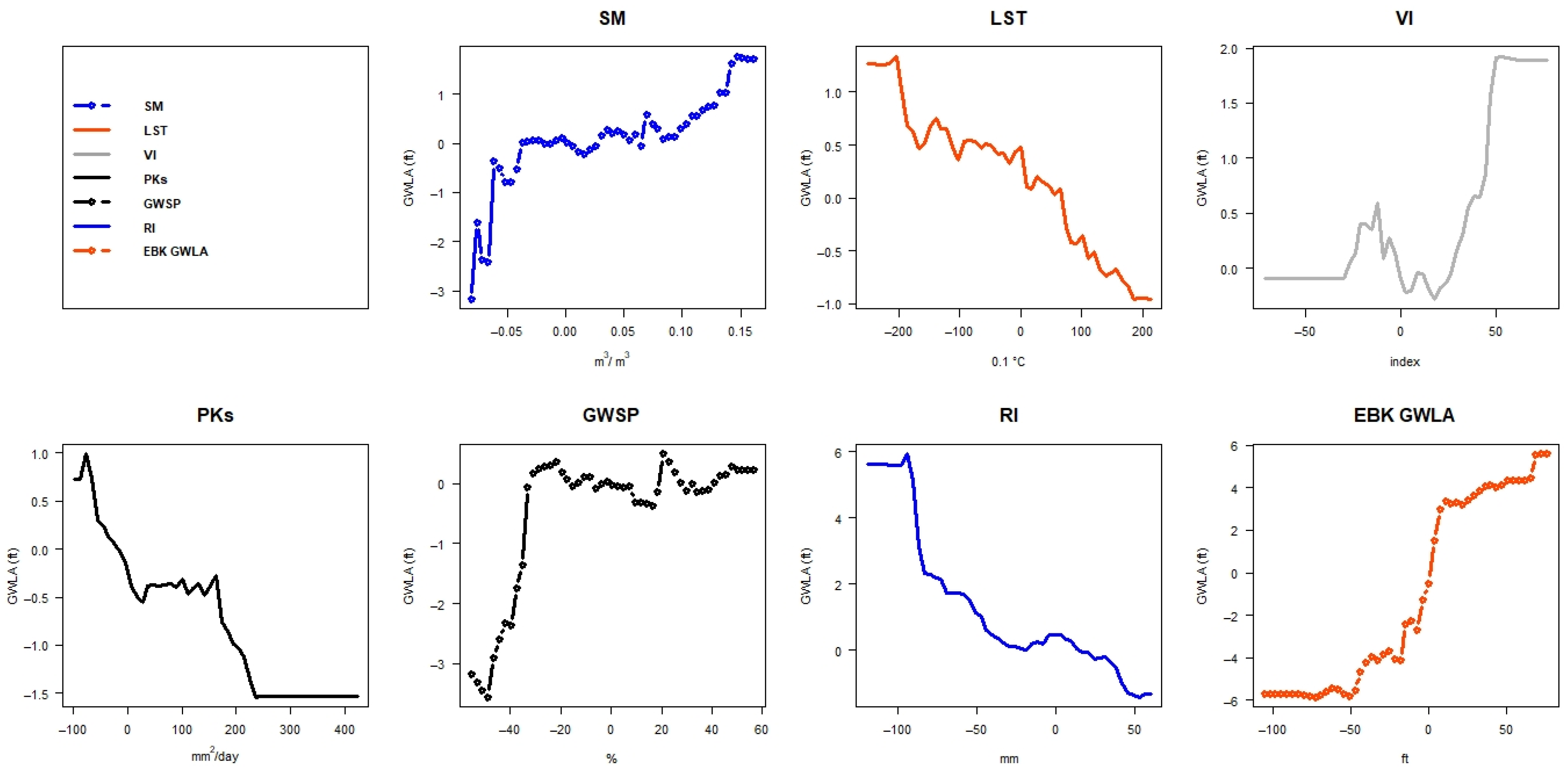
The partial dependence plots (Figure 11) describe the relationships between each of the seven predictors (while keeping the others constant) and the RF-model-predicted output. Recall that the RI variable was calculated based on the precipitation, evapotranspiration, and runoff depth values (Equation (4)) and that the runoff depths were derived from precipitation (Equations (1) and (2)), so it primarily reflects changes in evapotranspiration (Figure 11). Additionally, ET is influenced by LST, which explains why the RI and LST variables exhibited similar relationships with GWL (Figure 11).
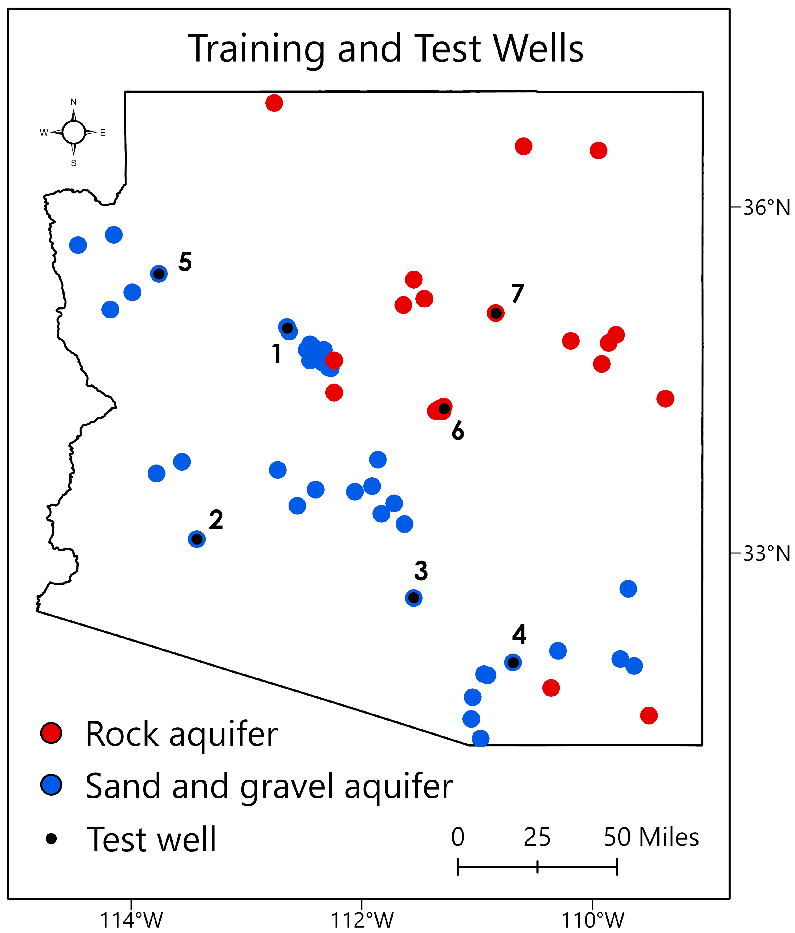
Following satisfactory validation performance, we repeated the EBK process using all 59 monitoring wells. As before, the interpolated GWL surfaces had a default grid size of 0.023° × 0.023°, likely determined by the geographical extent of the study area (Figure 12a). The standard errors of the prediction were also computed, with higher values representing larger prediction uncertainties (Figure 12b). The interpolated GWL surfaces were resampled to 0.125° × 0.125°, matching the grid size for this study (Figure 12c). Monthly anomalies were calculated (for each monitoring well) from the resampled surfaces and added to the dataset as a new predictor variable. A final RF model was developed using the complete augmented dataset, excluding seven wells reserved for testing (Figure 13).
For the third time in this study, the RF model showed much better predictions at locations with monitoring wells drilled into unconsolidated sand and gravel aquifers compared to those in rock aquifers (Table 5). The average NSE and R2 values are 0.88 and 0.92 for the former and 0.32 and 0.37 for the latter, respectively (Table 5).
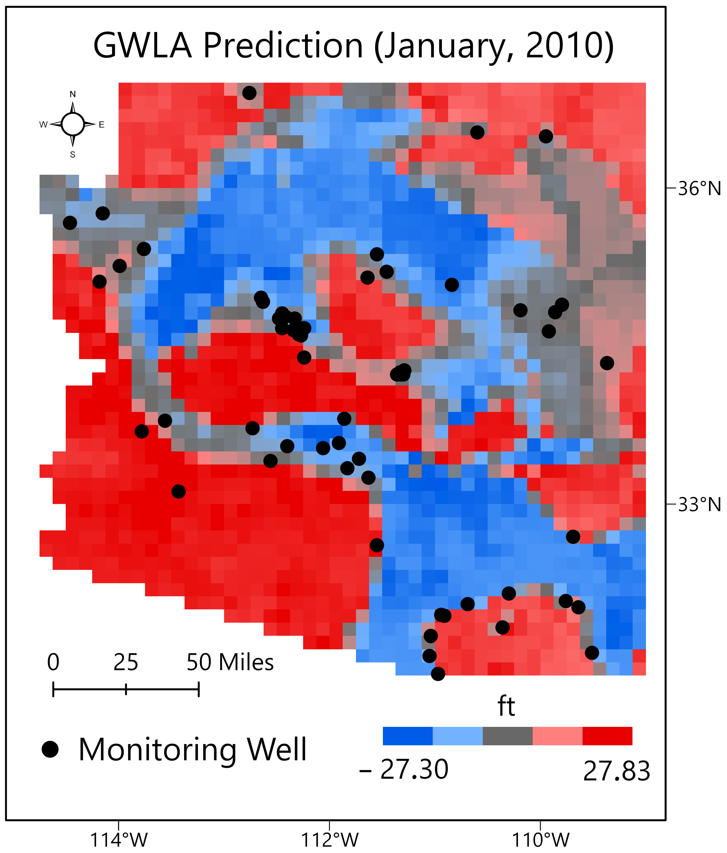
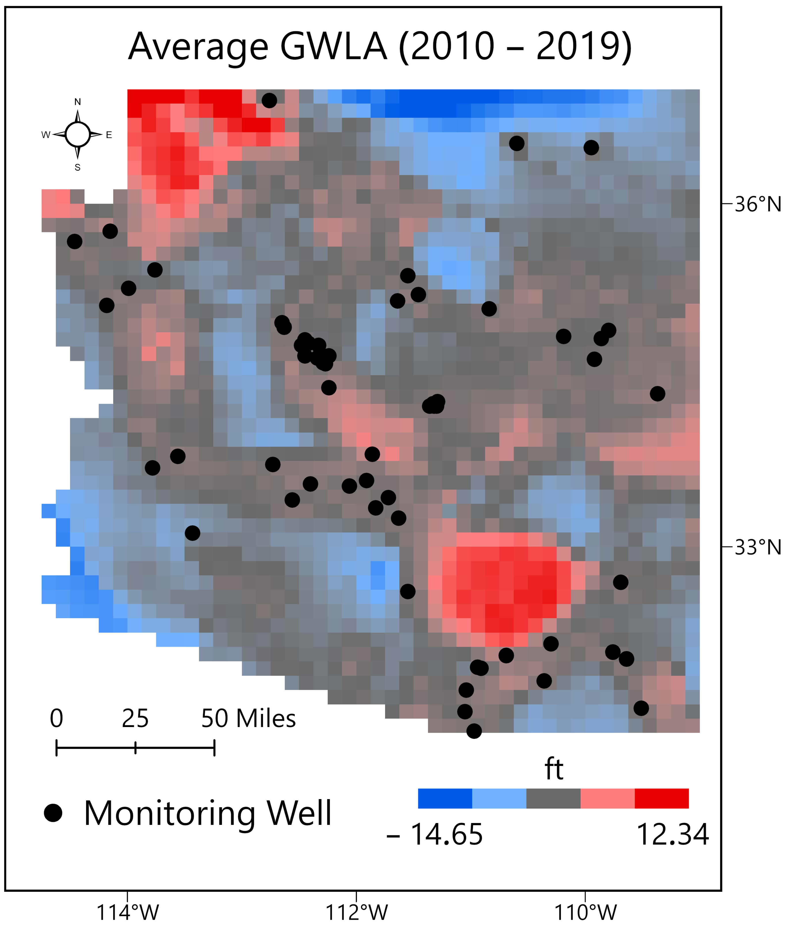
Following a satisfactory validation and test performance, we deployed the final RF model to make predictions at ungauged locations across the study area (Figure 14) and calculated the averages of those predictions for each 0.125° × 0.125° grid (Figure 15).

4. Discussion

Although ML is able to understand complex relationships between GWLs and contributing factors, this study revealed much better predictive performance for the unconsolidated material aquifers, where the relationships are generally more straightforward. Validation wells 1 and 3 were in close proximity to other wells (Figure 10) and could have benefited from the spatial autocorrelation of GWLs between them, but well 3 did not. In fact, validation well 2 performed better than well 3, despite not having that advantage (Figure 10, Table 4). This discrepancy may have been due to several factors, including the intricate heterogeneities and geologic structures in rock aquifers. The PDP for the PKs variable (Figure 11) also showed a distinction between the two aquifer types. This suggests that even with increased precipitation, changes in aquifer properties (such as reduced permeability in rock aquifers) can restrict groundwater flow and contribute to a declining GWL, considering all other factors at play. Both aquifers showed a negative relationship with PKs, but GWLs were relatively higher for the unconsolidated material aquifers (Figure 11). This shows that under similar hydrological conditions and assuming all other factors are kept constant, the properties of unconsolidated aquifer materials may allow them to maintain higher GWLs compared to rock aquifers.
The discrepancy in model performance could also have been due to both model and data limitations. RF, the most employed ML algorithm for GWL prediction [10], failed to effectively capture GWL trends in a dolomite rock aquifer in a semi-arid region [73] and was also outperformed in an aquifer with fractured hydrogeology in a similar climate [74], as shown by two separate studies. In both cases, deep learning (DL) models demonstrated the best performance. DL is a branch of ML that is based on the concept of deep neural networks and is especially known to outperform traditional (shallow) ML techniques in applications involving large amounts of data [75,76] and high dimensionality [75]. But drilling a large number of wells into hard rock formations in dry regions might not be practical for various reasons, including cost and limited water availability [77], which can pose significant challenges for ML-based GWL predictions in rock aquifers in arid regions. Specifically, fewer wells were drilled into the consolidated rocks in the study area compared to the basin fill unconsolidated materials [29], which potentially limited the adequate representation of the geologic complexities of these rock aquifers. However, the relatively weak performance of the RF models for the rock aquifers presents opportunities for future research to investigate and enhance the model performance in such complex geologic and climate settings. These efforts should begin with acquiring the maximum amount of good-quality data for a comprehensive analysis.
The prediction errors from the EBK models (Figure 12b) underscore the importance of the spatial density and distribution of the kriging data in ensuring the reliability of predictions. The largest uncertainties were seen around the boundaries of the study area, and the predictions in the vicinity of the monitoring wells were relatively more accurate. Two of the wells excluded in the validation phase (Figure 10) were included in the final model as test wells (Figure 13) and showed improved predictions (Table 4, Table 5), further underscoring the importance of data density and quality in kriging.
Based on the percent increases in the mean squared error (MSE) when important predictor variables are left out, the RI and EBK variables were the most important in the validation RF model, where both variables showed similar levels of importance. However, in the final deployment model, EBK was the most important variable (by a significant margin). This suggests that incorporating spatial interpolation techniques such as EBK can substantially enhance the performance of ML models. Although the kriging process can be tedious and challenging, the model improvements they offer make these efforts worth it.
As shown, the average GWLA for the period of study was predominantly negative. In fact, only about twenty-eight percent of the study area showed a positive average anomaly during this period. This trend reflects the challenges in a dry/arid region with high groundwater demand and withdrawal rates possibly exceeding natural recharge. Historically, groundwater in Arizona has been pumped out faster than it has been replenished by natural means [78,79], resulting in overdraft in many agricultural and urban areas [79]. But as the quest to exploit deeper aquifers continues, the costs of drilling to these depths are much higher, as are the energy costs of pumping water from them [79]. This study therefore could be useful for optimizing the drilling process by identifying locations for new wells and increasing the likelihood of accessing groundwater at optimal depths. Efforts to manage the groundwater overdraft issue began with identifying regions with a high reliance on groundwater (known as Active Management Areas (AMAs)) and subsequently empowering the ADWR to monitor compliance within the AMAs with the regulatory frameworks in place [79,80]. Within these AMAs and beyond, this study can also aid in the monitoring and allocation of groundwater resources by identifying groundwater-deficient areas based on the average predicted GWLA values, and offer data-driven support and recommendations towards the effective management of groundwater resources in vulnerable areas.

5. Conclusions

Groundwater is the largest reservoir of available freshwater in the world and a critically important resource. Its global relevance is amplified by the direct impacts of climate change on surface water sources, particularly in arid regions. In this study, we demonstrated the effectiveness of ML in predicting monthly GWLAs when combined with reliable spatial interpolation models and developed the first statewide GWLA prediction model for the state of Arizona. Following satisfactory performance based on average NSE/R2 values of 0.62/0.63 and 0.72/0.76 during the validation and testing phases, respectively, monthly GWLA rasters were produced for January 2010 to December 2019. Moving forward, future studies may focus on addressing some of the challenges of applying traditional ML techniques to rock aquifers in dry regions discussed in this study, in terms of leveraging the available data and reducing prediction uncertainties in such complex settings.
With well depths ranging from 25 to 1600 feet, this study demonstrated effectiveness for both shallow and deep aquifers. The model design utilized remotely sensed datasets from satellites with global coverage, enabling replicability for similar climates across the globe. Our remote sensing approach ensures that data-sparse regions of the world, where field-based hydrological variables are limited or largely inaccessible, are not left out. It is our hope that this work contributes substantially to the science of monitoring groundwater resources in the face of global warming and climate change threats, ensuring the availability of groundwater to meet domestic, agricultural, and industrial water needs.

Author Contributions

F.J.Z. was responsible for the conceptualization and methodology, analysis and interpretation of results, and the original draft preparation. A.M.M. supervised the project, and reviewed drafts of the manuscript. All authors have read and agreed to the published version of the manuscript.

Funding

This research was supported by the Miriam Watts-Wheeler Research Fund, awarded by the Department of Geology, the University of Georgia.

Data Availability Statement

The data presented in this study are available on request from the corresponding author.

Conflicts of Interest

The authors declare no conflicts of interest.

Abbreviations

The list of abbreviations and acronyms used in this paper are tabulated below:
ADWRArizona Department of Water Resources
AMAActive Management Area
ANNArtificial neural network
ARIMAAutoregressive integrated moving average
CONUSContiguous United States
CKClassical kriging
CNCurve number
CVCoefficient of variation
DLDeep learning
DTDecision tree
EBKEmpirical Bayesian kriging
ETEvapotranspiration
GBMGradient boosting mechanism
GIGeostatistical interpolation
GRACEGravity Recovery and Climate Experiment
GWLGroundwater level
GWLAGroundwater level anomaly
GWSPGroundwater storage percentile
KNNK-nearest neighbors
KsSoil saturated hydraulic conductivity
LSTLand surface temperature
MAEMean absolute error
MIMean imputation
MLMachine learning
MLRMultilinear regression
MSEMean squared error
NGWMNNational Groundwater Monitoring Network
PPrecipitation
PDPPartial dependence plot
PKsPrecipitation x soil saturated hydraulic conductivity
RRunoff depth
RBFRadial basis function
RBF-NNRadial basis function neural network
RBF-SVRRadial basis function support vector regression
RFRandom forest
RIRecharge index
RMSERoot mean square error
SMSoil moisture
SVMSupport vector machine
SVRSupport vector machine for regression
USGSU.S. Geological Survey
VIVegetation index
WCIWater cycle intensity

References

  1. Scanlon, B.R.; Keese, K.E.; Flint, A.L.; Flint, L.E.; Gaye, C.B.; Edmunds, W.M.; Simmers, I. Global synthesis of groundwater recharge in semiarid and arid regions. Hydrol. Process. 2006, 20, 3335–3370. [Google Scholar] [CrossRef]
  2. Dawoud, M.A. Groundwater economics in arid regions: Abu Dhabi Emirate case study. In Recent Advances in Environmental Science from the Euro-Mediterranean and Surrounding Regions, Proceedings of Euro-Mediterranean Conference for Environmental Integration (EMCEI-1), Sousse, Tunisia, 20–25 November 2017; Springer: Cham, Switzerland, 2017; pp. 611–613. [Google Scholar]
  3. Liu, Q.; Gui, D.; Zhang, L.; Niu, J.; Dai, H.; Wei, G.; Hu, B.X. Simulation of regional groundwater levels in arid regions using interpretable machine learning models. Sci. Total Environ. 2022, 831, 154902. [Google Scholar] [CrossRef] [PubMed]
  4. Haider, A.; Lee, G.; Jafri, T.H.; Yoon, P.; Piao, J.; Jhang, K. Enhancing Accuracy of Groundwater Level Forecasting with Minimal Computational Complexity Using Temporal Convolutional Network. Water 2023, 15, 4041. [Google Scholar] [CrossRef]
  5. Tao, H.; Hameed, M.M.; Marhoon, H.A.; Zounemat-Kermani, M.; Heddam, S.; Kim, S.; Sulaiman, S.O.; Tan, M.L.; Sa’adi, Z.; Mehr, A.D.; et al. Groundwater level prediction using machine learning models: A comprehensive review. Neurocomputing 2022, 489, 271–308. [Google Scholar] [CrossRef]
  6. Ardana, P.D.H.; Redana, I.W.; Yekti, M.I.; Simpen, I.N. Groundwater Level Forecasting Using Multiple Linear Regression and Artificial Neural Network Approaches. Civ. Eng. Archit. 2022, 10, 784–799. [Google Scholar] [CrossRef]
  7. Najafabadipour, A.; Kamali, G.; Nezamabadi-Pour, H. Application of Artificial Intelligence Techniques for the Determination of Groundwater Level Using Spatio–Temporal Parameters. ACS Omega 2022, 7, 10751–10764. [Google Scholar] [CrossRef]
  8. Sahoo, M.; Kasot, A.; Dhar, A.; Kar, A. On predictability of groundwater level in shallow wells using satellite observations. Water Resour. Manag. 2018, 32, 1225–1244. [Google Scholar] [CrossRef]
  9. Li, B.; Yang, G.; Wan, R.; Dai, X.; Zhang, Y. Comparison of random forests and other statistical methods for the prediction of lake water level: A case study of the Poyang Lake in China. Hydrol. Res. 2016, 47 (Suppl. S1), 69–83. [Google Scholar] [CrossRef]
  10. Afrifa, S.; Zhang, T.; Appiahene, P.; Varadarajan, V. Mathematical and machine learning models for groundwater level changes: A systematic review and bibliographic analysis. Future Internet 2022, 14, 259. [Google Scholar] [CrossRef]
  11. Gonzalez, R.Q.; Arsanjani, J.J. Prediction of groundwater level variations in a changing climate: A Danish case study. ISPRS Int. J. Geo-Inf. 2021, 10, 792. [Google Scholar] [CrossRef]
  12. Guzman, S.M.; Paz, J.O.; Tagert, M.L.M.; Mercer, A.E. Evaluation of seasonally classified inputs for the prediction of daily groundwater levels: NARX networks vs support vector machines. Environ. Model. Assess. 2019, 24, 223–234. [Google Scholar] [CrossRef]
  13. Yoon, H.; Hyun, Y.; Ha, K.; Lee, K.K.; Kim, G.B. A method to improve the stability and accuracy of ANN-and SVM-based time series models for long-term groundwater level predictions. Comput. Geosci. 2016, 90, 144–155. [Google Scholar] [CrossRef]
  14. Behzad, M.; Asghari, K.; Coppola, E.A., Jr. Comparative study of SVMs and ANNs in aquifer water level prediction. J. Comput. Civ. Eng. 2010, 24, 408–413. [Google Scholar] [CrossRef]
  15. Nie, S.; Bian, J.; Wan, H.; Sun, X.; Zhang, B. Simulation and uncertainty analysis for groundwater levels using radial basis function neural network and support vector machine models. Res. Technol.—AQUA 2017, 66, 15–24. [Google Scholar] [CrossRef]
  16. Tapak, L.; Rahmani, A.R.; Moghimbeigi, A. Prediction the groundwater level of Hamadan-Bahar plain, west of Iran using support vector machines. J. Res. Health Sci. 2013, 14, 82–87. [Google Scholar]
  17. Tiwari, V.; Verma, M. Prediction of Groundwater Level Using Advance Machine Learning Techniques. In Proceedings of the 3rd IEEE International Conference on Intelligent Technologies (CONIT), Hubli, India, 23–25 June 2023; pp. 1–6. [Google Scholar]
  18. Hikouei, I.S.; Eshleman, K.N.; Saharjo, B.H.; Graham, L.L.; Applegate, G.; Cochrane, M.A. Using machine learning algorithms to predict groundwater levels in Indonesian tropical peatlands. Sci. Total Environ. 2023, 857, 159701. [Google Scholar] [CrossRef]
  19. Kanyama, Y.; Ajoodha, R.; Seyler, H.; Makondo, N.; Tutu, H. Application of machine learning techniques in forecasting groundwater levels in the grootfontein aquifer. In Proceedings of the 2nd IEEE International Multidisciplinary Information Technology and Engineering Conference (IMITEC), Kimberley, South Africa, 25–27 November 2020; pp. 1–8. [Google Scholar]
  20. Alam, M.J.; Kar, S.; Zaman, S.; Ahamed, S.; Samiya, K. Forecasting Underground Water Levels: LSTM Based Model Outperforms GRU and Decision Tree Based Models. In Proceedings of the IEEE International Women in Engineering (WIE) Conference on Electrical and Computer Engineering (WIECON-ECE), Naya Raipur, India, 30–31 December 2022; pp. 280–283. [Google Scholar]
  21. Biernacik, P.; Kazimierski, W.; Włodarczyk-Sielicka, M. Comparative Analysis of Selected Geostatistical Methods for Bottom Surface Modeling. Sensors 2023, 23, 3941. [Google Scholar] [CrossRef]
  22. Manda, S.; Patil, A. Analysis of groundwater level differences in Ganges basin using geostatistical modeling. Int. J. Agric. Eng. 2018, 11, 392–396. [Google Scholar] [CrossRef]
  23. Krivoruchko, K. Empirical bayesian kriging. ArcUser Fall 2012, 6, 1145. [Google Scholar]
  24. Bouhout, S.; Haboubi, K.; Zian, A.; Elyoubi, M.S.; Elabdouni, A. Evaluation of two linear kriging methods for piezometric levels interpolation and a framework for upgrading groundwater level monitoring network in Ghiss-Nekor plain, north-eastern Morocco. Arab. J. Geosci. 2022, 15, 1016. [Google Scholar] [CrossRef]
  25. Hussain, M.M.; Bari, S.H.; Tarif, M.E.; Rahman, M.T.U.; Hoque, M.A. Temporal and spatial variation of groundwater level in Mymensingh district, Bangladesh. Int. J. Hydrol. Sci. Technol. 2016, 6, 188–197. [Google Scholar] [CrossRef]
  26. Deshmukh, M.M.; Elbeltagi, A.; Kouadri, S. Climate Change Impact on Groundwater Resources in Semi-arid Regions. In Climate Change Impact on Groundwater Resources: Human Health Risk Assessment in Arid and Semi-Arid Regions; Panneerselvam, B., Pande, C.B., Muniraj, K., Balasubramanian, A., Ravichandran, N., Eds.; Springer: Cham, Switzerland, 2022; pp. 9–23. [Google Scholar]
  27. Zowam, F.J.; Milewski, A.M.; Richards IV, D.F. A Satellite-Based Approach for Quantifying Terrestrial Water Cycle Intensity. Remote Sens. 2023, 15, 3632. [Google Scholar] [CrossRef]
  28. McCafferty, A.E.; San Juan, C.A.; Lawley, C.J.M.; Graham, G.E.; Gadd, M.G.; Huston, D.L.; Kelley, K.D.; Paradis, S.; Peter, J.M.; Czarnota, K. National-Scale Geophysical, Geologic, and Mineral Resource Data and Grids for the United States, Canada, and Australia: Data in Support of the Tri-National Critical Minerals Mapping Initiative: US Geological Survey Data Release. Available online: https://www.sciencebase.gov/catalog/item/623a013ed34e915b67cddcfa (accessed on 22 February 2024).
  29. Bedinger, M.S.; Anderson, T.W.; Langer, W.H. Groundwater Units and Withdrawal, Basin and Range Province, Arizona. Water-Resources Investigations Report (No. 83-4114-A); U.S. Geological Survey: Reston, VA, USA, 1984. [Google Scholar] [CrossRef]
  30. Tillman, F.D.; Flynn, M.E. Arizona Groundwater Explorer: Interactive maps for evaluating the historical and current groundwater conditions in wells in Arizona, USA. Hydrogeol. J. 2024, 32, 645–661. [Google Scholar] [CrossRef]
  31. Bertsimas, D.; Pawlowski, C.; Zhuo, Y.D. From predictive methods to missing data imputation: An optimization approach. J. Mach. Learn. Res. 2018, 18, 1–39. [Google Scholar]
  32. Petrazzini, B.O.; Naya, H.; Lopez-Bello, F.; Vazquez, G.; Spangenberg, L. Evaluation of different approaches for missing data imputation on features associated to genomic data. BioData Min. 2021, 14, 1–13. [Google Scholar] [CrossRef] [PubMed]
  33. Muharemi, F.; Logofătu, D.; Leon, F. Review on general techniques and packages for data imputation in R on a real world dataset. In Computational Collective Intelligence, Proceedings of the 10th International Conference, Bristol, UK, 5–7 September 2018; Part II 10; Springer International Publishing: Cham, Switzerland, 2018; pp. 386–395. [Google Scholar]
  34. Lande, R. On comparing coefficients of variation. Syst. Zool. 1977, 26, 214–217. [Google Scholar] [CrossRef]
  35. Seyoum, W.M.; Kwon, D.; Milewski, A.M. Downscaling GRACE TWSA data into high-resolution groundwater level anomaly using machine learning-based models in a glacial aquifer system. Remote Sens. 2019, 11, 824. [Google Scholar] [CrossRef]
  36. Moeck, C.; Grech-Cumbo, N.; Podgorski, J.; Bretzler, A.; Gurdak, J.J.; Berg, M.; Schirmer, M. A global-scale dataset of direct natural groundwater recharge rates: A review of variables, processes and relationships. Sci. Total Environ. 2020, 717, 137042. [Google Scholar] [CrossRef]
  37. Pradhan, R.K.; Markonis, Y.; Godoy, M.R.V.; Villalba-Pradas, A.; Andreadis, K.M.; Nikolopoulos, E.I.; Papalexiou, S.M.; Rahim, A.; Tapiador, F.J.; Hanel, M. Review of GPM IMERG performance: A global perspective. Remote Sens. Environ. 2022, 268, 112754. [Google Scholar] [CrossRef]
  38. Milewski, A.; Elkadiri, R.; Durham, M. Assessment and comparison of TMPA satellite precipitation products in varying climatic and topographic regimes in Morocco. Remote Sens. 2015, 7, 5697–5717. [Google Scholar] [CrossRef]
  39. Mohammed, S.A.; Hamouda, M.A.; Mahmoud, M.T.; Mohamed, M.M. Performance of GPM-IMERG precipitation products under diverse topographical features and multiple-intensity rainfall in an arid region. Hydrol. Earth Syst. Sci. 2020, 2020, 1–27. [Google Scholar]
  40. Huffman, G.J.; Bolvin, D.T.; Braithwaite, D.; Hsu, K.; Joyce, R.; Xie, P.; Yoo, S.H. NASA global precipitation measurement (GPM) integrated multi-satellite retrievals for GPM (IMERG). Algorithm Theor. Basis Doc. (ATBD) 2015, 4, 30. [Google Scholar]
  41. Malik, M.S.; Shukla, J.P.; Mishra, S. Effect of groundwater level on soil moisture, soil temperature and surface temperature. J. Indian Soc. Remote Sens. 2021, 49, 2143–2161. [Google Scholar] [CrossRef]
  42. Maihemuti, B.; Simayi, Z.; Alifujiang, Y.; Aishan, T.; Abliz, A.; Aierken, G. Development and evaluation of the soil water balance model in an inland arid delta oasis: Implications for sustainable groundwater resource management. Glob. Ecol. Conserv. 2021, 25, e01408. [Google Scholar] [CrossRef]
  43. Otoko, G.R. Mathematical Relationship between Soil Moisture and Groundwater Level in A Loamy Sand Soil in The Niger Delta Region of Nigeria. Int. J. Adv. Res. Sci. Eng. Technol. 2014, 5, 1–8. [Google Scholar]
  44. Hongtao, J.; Huanfeng, S.; Xinghua, L.; Lili, L. The 43-Year (1978–2020) Global 9 km Remotely Sensed Soil Moisture Product: PANGAEA. Available online: https://doi.org/10.1594/PANGAEA.940409 (accessed on 12 February 2023).
  45. Elnashar, A.; Wang, L.; Wu, B.; Zhu, W.; Zeng, H. Synthesis of global actual evapotranspiration from 1982 to 2019. Earth Syst. Sci. Data 2021, 13, 447–480. [Google Scholar] [CrossRef]
  46. Zhang, T.; Zhou, Y.; Zhu, Z.; Li, X.; Asrar, G.R. A global seamless 1 km resolution daily land surface temperature dataset (2003–2020). Earth Syst. Sci. Data 2021, 2021, 651–664. [Google Scholar] [CrossRef]
  47. Grove, M.; Harbor, J.; Engel, B. composite vs. distributed curve numbers: Effects on estimates of storm runoff depths. J. Am. Water Resour. Assoc. 1998, 34, 1015–1023. [Google Scholar] [CrossRef]
  48. Arisanty, D.; Rahmawati, N.; Rosadi, D. Soil Physical Characteristics and Saturated Hydraulic Conductivity in the Landform of Barito Delta, Kalimantan, Indonesia. Appl. Environ. Soil Sci. 2022, 2022, 9118461. [Google Scholar] [CrossRef]
  49. Gupta, S.; Lehmann, P.; Bonetti, S.; Papritz, A.; Or, D. Global prediction of soil saturated hydraulic conductivity using random forest in a covariate-based geoTransfer function (CoGTF) framework. J. Adv. Model. Earth Syst. 2021, 13, e2020MS002242. [Google Scholar] [CrossRef]
  50. Beaudoing, H.; Rodell, M.; Getirana, A.; Li, B. Groundwater and Soil Moisture Conditions from GRACE and GRACE-FO Data Assimilation L4 7-Days 0.125 × 0.125 Degree U.S. V4.0; Goddard Earth Sciences Data and Information Services Center (GES DISC): Greenbelt, MD, USA, 2021. Available online: https://disc.gsfc.nasa.gov/datasets/GRACEDADM_CLSM0125US_7D_4.0/summary (accessed on 30 October 2023).
  51. Dhungel, R.; Fiedler, F. Water balance to recharge calculation: Implications for watershed management using systems dynamics approach. Hydrology 2016, 3, 13. [Google Scholar] [CrossRef]
  52. Ahmadi, A.; Olyaei, M.; Heydari, Z.; Emami, M.; Zeynolabedin, A.; Ghomlaghi, A.; Daccache, A.; Fogg, G.E.; Sadegh, M. Groundwater level modeling with machine learning: A systematic review and meta-analysis. Water 2022, 14, 949. [Google Scholar] [CrossRef]
  53. Ding, J.; Tarokh, V.; Yang, Y. Model selection techniques: An overview. IEEE Signal Process. Mag. 2018, 35, 16–34. [Google Scholar] [CrossRef]
  54. Vapnik, V.N. An overview of statistical learning theory. IEEE Trans. Neural Netw. 1999, 10, 988–999. [Google Scholar] [CrossRef] [PubMed]
  55. Awad, M.; Khanna, R. Support Vector Machines for Classification. In Efficient Learning Machines; Apress: Berkeley, CA, USA, 2015; p. 268. [Google Scholar]
  56. Drucker, H.; Burges, C.J.; Kaufman, L.; Smola, A.; Vapnik, A. Support vector regression machines. Adv. Neural. Inf. Process Syst. 1996, 9, 161–226. [Google Scholar]
  57. Amirkhalili, Y.S.; Aghsami, A.; Jolai, F. Comparison of Time Series ARIMA Model and Support Vector Regression. Int. J. Hybrid Inf. Technol. 2020, 13, 7–18. [Google Scholar] [CrossRef]
  58. Ranković, V.; Grujović, N.; Divac, D.; Milivojević, N. Development of support vector regression identification model for prediction of dam structural behaviour. Struct. Saf. 2014, 48, 33–39. [Google Scholar] [CrossRef]
  59. Ayodeji, A.; Liu, Y.K. SVR optimization with soft computing algorithms for incipient SGTR diagnosis. Ann. Nucl. Energy 2018, 121, 89–100. [Google Scholar] [CrossRef]
  60. Açıkkar, M.; Altunkol, Y. A novel hybrid PSO-and GS-based hyperparameter optimization algorithm for support vector regression. Neural Comput. 2023, 35, 19961–19977. [Google Scholar] [CrossRef]
  61. Kuhn, M.; Johnson, K. Applied Predictive Modeling; Springer: New York, NY, USA, 2013. [Google Scholar]
  62. Al-Anazi, A.F.; Gates, I.D. Support vector regression for porosity prediction in a heterogeneous reservoir: A comparative study. Comput. Geosci. 2010, 36, 1494–1503. [Google Scholar] [CrossRef]
  63. Kavousi-Fard, A.; Samet, H.; Marzbani, F. A new hybrid modified firefly algorithm and support vector regression model for accurate short term load forecasting. Expert Syst. Appl. 2014, 41, 6047–6056. [Google Scholar] [CrossRef]
  64. Karatzoglou, A.; Meyer, D.; Hornik, K. Support vector machines in R. J. Stat. Softw. 2006, 15, 1–28. [Google Scholar] [CrossRef]
  65. Kaneko, H.; Funatsu, K. Fast optimization of hyperparameters for support vector regression models with highly predictive ability. Chemom. Intell. Lab. Syst. 2015, 142, 64–69. [Google Scholar] [CrossRef]
  66. Tsirikoglou, P.; Abraham, S.; Contino, F.; Lacor, C.; Ghorbaniasl, G. A hyperparameters selection technique for support vector regression models. Appl. Soft Comput. 2017, 61, 139–148. [Google Scholar] [CrossRef]
  67. Breiman, L. Random forests. Mach. Learn. 2001, 45, 5–32. [Google Scholar] [CrossRef]
  68. Wu, D.J.; Feng, T.; Naehrig, M.; Lauter, K. Privately evaluating decision trees and random forests. Proc. Priv. Enh. Technol. 2015, 2016, 335–355. [Google Scholar] [CrossRef]
  69. Liaw, A.; Wiener, M. Classification and regression by randomForest. R News 2002, 2, 18–22. [Google Scholar]
  70. Rigatti, S.J. Random forest. J. Insur. Med. 2017, 47, 31–39. [Google Scholar] [CrossRef]
  71. Maliva, R.G. Geostatistical methods and applications. In Aquifer Characterization Techniques; Springer: Cham, Switzerland, 2016; No. 4; pp. 595–617. [Google Scholar]
  72. Li, Y.; Hernandez, J.H.; Aviles, M.; Knappett, P.S.; Giardino, J.R.; Miranda, R.; Puy, M.J.; Padilla, F. Morales, J. Empirical Bayesian Kriging method to evaluate inter-annual water-table evolution in the Cuenca Alta del Río Laja aquifer, Guanajuato, México. J. Hydrol. 2020, 582, 124517. [Google Scholar] [CrossRef]
  73. Kanyama, Y. Application of Machine Learning Techniques in Predicting Groundwater Levels and Discharge Rates in the Northwest Aquifers. Master’s Thesis, The University of the Witwatersrand, Johannesburg, South Africa, 22 April 2021. [Google Scholar]
  74. Yin, W.; Fan, Z.; Tangdamrongsub, N.; Hu, L.; Zhang, M. Comparison of physical and data-driven models to forecast groundwater level changes with the inclusion of GRACE–A case study over the state of Victoria, Australia. J. Hydrol. 2021, 602, 126735. [Google Scholar] [CrossRef]
  75. Janiesch, C.; Zschech, P.; Heinrich, K. Machine learning and deep learning. Electron. Mark. 2021, 31, 685–695. [Google Scholar] [CrossRef]
  76. Xu, Y.; Zhou, Y.; Sekula, P.; Ding, L. Machine learning in construction: From shallow to deep learning. Dev. Built Environ. 2021, 6, 100045. [Google Scholar] [CrossRef]
  77. Sk, M.; Ramanujam, N.; Champoil, V.; Biswas, S.K.; Rasool, Q.A.; Ojha, C. Identification of groundwater in hard rock terrain using 2D electrical resistivity tomography imaging technique: Securing water scarcity at the time of seasonal rainfall failure, South Andaman. Int. J. Geosci. 2018, 9, 59. [Google Scholar] [CrossRef]
  78. Arizona Department of Water Resources. Overview of the Arizona Groundwater Management Code. Available online: https://www.azwater.gov/sites/default/files/media/Arizona%20Groundwater_Code_1.pdf (accessed on 14 June 2024).
  79. Hirt, P.; Snyder, R.; Hester, C.; Larson, K. Water consumption and sustainability in Arizona: A tale of two desert cities. J. Southwest 2017, 59, 264–301. [Google Scholar] [CrossRef]
  80. Megdal, S.B. Arizona groundwater management. Water Rep. 2012, 104, 9–15. [Google Scholar]
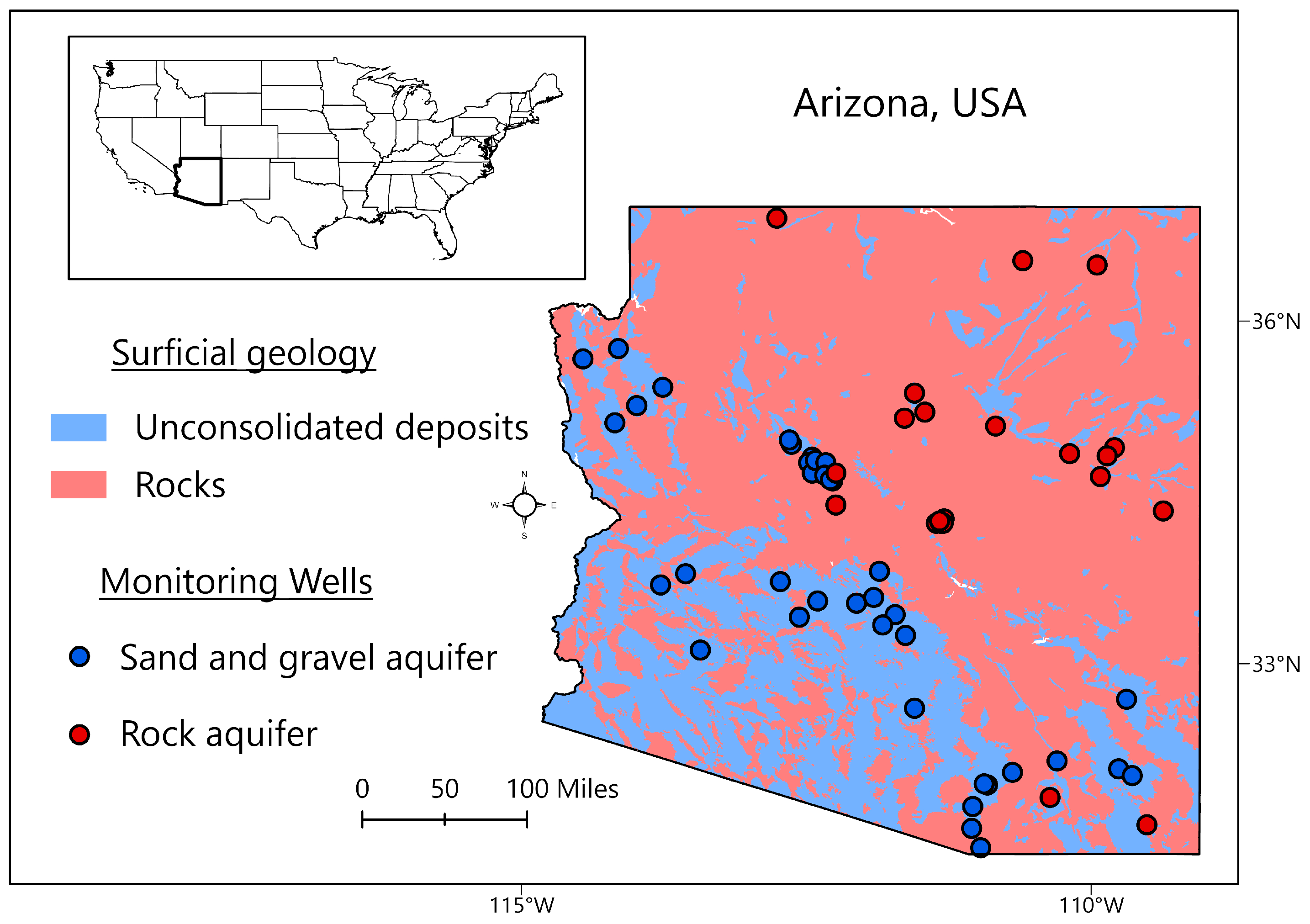
Figure 1. Map of the study area showing the locations of groundwater monitoring wells.
Water 16 02771 g001
Figure 2. Maps of initial predictor variables resampled to 0.125° × 0.125° grid resolution. P = precipitation, SM = soil moisture, ET = evapotranspiration, LST = land surface temperature, VI = vegetation index, CN = curve number, K = saturated hydraulic conductivity, and GWSP = groundwater storage percentile. CN and K are representative values for the period of study, and all the other variables are for January 2010.
Water 16 02771 g002
Figure 3. One-dimensional SVR, where x is the input or independent variable and y is the dependent variable. Source: Awad and Khanna (2015) [55].
Water 16 02771 g003
Figure 4. A simple RF model with three DTs.
Water 16 02771 g004
Figure 5. (a) A single semivariogram. Source: Maliva (2016) [71]. (b) The EBK model showing a distribution of semivariograms. Source: Krivoruchko (2012) [23]. The red dotted lines represent the lower and upper quartiles, and the solid red line represents the median of the semivariogram distribution [23,72].
Water 16 02771 g005
Figure 6. Model design showing train/test split ratios for the spatial (a) and temporal (b) evaluations and the locations of the split wells.
Water 16 02771 g006
Figure 7. RF schematic with three observations, the seven predictor variables, three randomly selected predictors to build each tree, and three DTs. The target variable is shown in blue, and the predicted outputs are shown in red.
Water 16 02771 g007
Figure 8. Map showing the locations of the four test wells for temporal evaluations after the second (85:15) train/test split.
Water 16 02771 g008
Figure 9. Plots comparing the RF-predicted GWLA at each test well with observed values. The numbers 1–4 correspond to the four test wells shown in Figure 8 and Table 3.
Water 16 02771 g009
Figure 10. Location of the validation wells (1–3). The validation wells were removed from the dataset before performing the EBK to ensure unbiased model evaluation.
Water 16 02771 g010
Figure 11. Partial dependence plots (PDPs) of the validation RF model. Each plot illustrates the relationship between the given predictor variable and the predicted output, showing how changes in the former influence the latter.
Water 16 02771 g011
Figure 12. EBK model output for January 2010 showing (a) GWL predictions at 0.023° × 0.023°, (b) standard errors of those predictions at 0.023° × 0.023°, and (c) resampled GWL prediction surface at a 0.125° × 0.125° grid size.
Water 16 02771 g012
Figure 13. Spatial locations of all the monitoring wells used in this study. Wells 1–7 were used to evaluate the performance of the final RF model.
Water 16 02771 g013
Figure 14. GWLA predictions for January 2010 after model deployment. The monitoring wells (black circles) represent both training and test wells for the final RF model.
Water 16 02771 g014
Figure 15. Average GWLA for the period of study (January 2010 to December 2019), and the locations of the monitoring wells (black circles) used in this study.
Water 16 02771 g015
Table 1. Final input variables used in the study and the processing involved.
IDVariableProcessingUnit
1Soil moisture (SM)× ○m3/m3
2Land surface temperature (LST)× ∆ ○°C
3Vegetation index (VI)
4Saturated hydraulic conductivity (PKs) *○ ∆ □mm2/day
5Groundwater storage percentile (GWSP) %
6Recharge index (RI) *○ | ○ | □mm
Note(s): × = convert daily data into monthly averages; ∆ = raster averaging; ○ = resampling to 0.125° × 0.125°; □ = raster arithmetic operations. NB: Secondary variables are marked with an asterisk (*), and the pipe symbol (|) separates the processing applied to each individual variable.
Table 2. Performance of individual SVR models.
ModelNSER2
1January
2February 0.880.88
3March 0.710.71
4April 0.510.51
5May 0.870.89
6June 0.900.93
7July 0.960.97
8August 0.870.87
9September 0.800.81
10October 0.770.78
11November 0.830.83
12December 0.910.92
Table 3. RF model performance evaluated at the four test wells (15 percent test split).
IDTest WellAquifer TypeNSER2
1Artesia School [D-08-26 33CDC1]Sand and gravel0.870.87
2Geiler [B-16-02 21BAA2]Sand and gravel0.800.80
3Queen Creek [D-02-07 22BBC]Sand and gravel0.840.87
4PE–11 [A-10-10 11ACB]Rock−0.130.28
Table 4. RF model performance at validation wells using the EBK predictions as input.
IDValidation WellAquifer TypeNSER2
1Antelope Wash [B-18-04 25AAA2]Sand and gravel0.810.83
2Turtleback [C-03-11 31DBB]Sand and gravel0.630.65
3Rumsey Park [A-10-10 04ABB]Rock0.410.41
Table 5. RF model performance using all monitoring wells for EBK predictions. Test wells marked with an asterisk (*) indicate that they were also used for validation.
IDTest WellAquifer TypeNSER2
1Antelope Wash [B-18-04 25AAA2] *Sand and gravel0.980.99
2Turtleback [C-03-11 31DBB] *Sand and gravel0.860.88
3Friendly Corners [D-09-08 29BCC]Sand and gravel0.820.87
4Pantano Wash North [D-16-16 15ABD]Sand and gravel0.880.94
5Truxton South [B-24-14 33ADA]Sand and gravel0.840.90
6GC–3 [A-11-10 26DAB]Rock0.440.46
7[A-19-14 03AAC1]Rock0.200.28
Disclaimer/Publisher’s Note: The statements, opinions and data contained in all publications are solely those of the individual author(s) and contributor(s) and not of MDPI and/or the editor(s). MDPI and/or the editor(s) disclaim responsibility for any injury to people or property resulting from any ideas, methods, instructions or products referred to in the content.