Abstract
A concurrent heuristic search iterative process (CHSIP) is used for estimating groundwater pollution sources and aquifer parameters in this work. Frequent calls to carry out a numerical simulation of groundwater pollution have generated a huge calculated load during the CHSIP. Therefore, a valid means to mitigate this is building a substitute to emulate the numerical simulation at a low calculated load. However, there is a complicated nonlinear correlativity between the import and export of the numerical simulation on account of the large quantity of variables. This leads to a poor approach accuracy of the substitute compared to the simulation when using shallow learning methods. Therefore, we first built a stacked autoencoder substitute, using the deep learning method, to boost the approach accuracy of the substitute compared to the numerical simulation. In total, 400 training samples and 100 testing samples for the substitute were collected by employing the Latin hypercube sampling method and running the numerical simulator. The CHSIP was then employed for estimating the groundwater pollution sources and aquifer parameters, and the estimated outcome was obtained when the CHSIP was terminated. The data analysis, including interval estimation and point estimation, was implemented on the MATLAB platform. A relevant hypothetical case is set to verify our approaches, which shows that the CHSIP is helpful for estimating the groundwater pollution source and aquifer parameters and that the stacked autoencoder method can effectively boost the approach precision of the substitute for the simulator.
1. Introduction
Groundwater polluted source estimation (GPSE) has important research value and practical significance in the increasingly serious problem of pollution at present [1,2,3,4]. Furthermore, the specific circumstance of aquifer parameters is also unknown in real pollution cases. Therefore, the groundwater pollution source and aquifer parameters are regarded as unknown variables and are estimated together [5,6]. The random statistics method is commonly used to handle the GPSE [7,8]. We proposed a concurrent heuristic search iterative process (CHSIP) according to the random statistics method to handle the GPSE, and each iteration included selecting the starting and candidate points [9,10,11]. Finally, the truth values of unknown variables could be found through the CHSIP based on the initial estimations. Therefore, we utilized the CHSIP to resolve the GPSE in this paper.
The numerical simulator of groundwater pollution needs to be repeatedly called upon during the CHSIP while solving the GPSE, which will incur a huge amount of computational load. Using a replacement to replace the numerical simulator can effectively handle this problem. The methodology for establishing a substitute presently includes the radial basis function (RBF) method and Gaussian process (GP) method, all of which are shallow machine learning methods [12,13,14]. Particularly, the GP method is a shallow learning method originating from geo-statistics. Based on the construction of known sample information, the GP method constructs an approximate function to predict the information of an unknown point. The GP method has long been introduced into the construction of a substitute and has been widely used. But the import variable and export variable of the mathematical simulator have a complicated nonlinear correlativity, owing to many variables. The shallow neural networks are unable to match the complicated nonlinear correlativity well; thus, is it difficult for the approach accuracy of the substitute for a simulator, which uses shallow learning methods, to meet the requirements [15,16,17]. Therefore, the need for a methodology to improve the approximation precision has become an urgent problem to be addressed. Owing to the rapid expansion of artificial intelligence, the deep learning method based on artificial intelligence has shown huge potential in fitting complicated nonlinear correlativity [18,19,20]. The stacked autoencoder (SAE) method is a popular deep learning method, and we first employ the SAE method to set up an SAE substitute for the mathematical simulation of groundwater pollution to enhance the approximation precision. The feature extraction ability of the SAE has been improved by stacking several autoencoders (AEs) for the unsupervised greedy training layer by layer [6,21,22]. Concomitantly, the ability of fitting the complicated nonlinear correlativity of the SAE has been enhanced by increasing the number of AEs and increasing the depth of the SAE structure. Further, the approach accuracy of the SAE substitute for the mathematical simulation has been enhanced.
This work focuses on (1) a case of groundwater pollution is designed and the corresponding established numerical simulator. Then, (2) the GP and the SAE substitutes of the numerical simulator are established. Subsequently, (3) the approach accuracy of the GP and the SAE substitutes for the mathematical simulation are contrasted and the substitute with highest approach accuracy is chosen as the final substitute of the simulation. Thereafter, (4) the CHSIP is carried out for the GPSE, and finally, (5) the unknown variables are estimated.
2. Methodology
2.1. The Mathematical Simulator
It is only possible to determine a mathematical simulation of a groundwater flow problem based on ascertaining hydrogeological conditions. To facilitate the problem, we usually ignore some secondary factors that have little to do with the case study. On this basis, we can build a conceptual model of the case study with a generalization of the hydrogeological conditions. Then, starting from this conceptual model, a simple mathematical language is used for depicting the quantitative relationship and spatial form of the conceptual model to reflect the hydrogeological conditions of the case study and the basic characteristics of the groundwater movement, eventually achieving the purpose of reproducing the basic state of the actual groundwater flow system. Such a mathematical structure is a mathematical simulator.
The mathematical simulator of groundwater includes the mathematical simulator describing the movement of groundwater and the mathematical simulator describing the movement of groundwater pollution. The mathematical simulator describing the movement of groundwater is described as follows:
where li and lj represent the location distances along the respective coordinate axis; H denotes the groundwater level; Kij denotes the tensor of hydraulic conductivity (also called the tensor of permeability coefficient).
The mathematical simulator describing movement of groundwater pollution is described as follows:
where represents the dispersity tensor; represents effective porosity; t represents time; represents average linear velocity; represents groundwater pollution concentration; and d represents aquifer thickness. The computing module of MODFLOW in the Groundwater Modeling System software (Version 10.8) is employed for solving the mathematical simulation describing the groundwater movement. And the MT3DMS module is used for solving the mathematical simulation describing the groundwater pollution movement.
2.2. The SAE Substitute
The stacked autoencoder (SAE) belongs to the deep neural net (DNN) method. By adding the depth of the net structure, i.e., establishing a multi-layer neural net construction with multiple hidden layers, the DNN can accurately extract the characteristics layer by layer and enhance the predicting capacity. Compared with a shallow neural network, a deep neural net has deeper network construction and stronger feature extraction capacity.
The SAE neural network is composed of cascades of multiple self-encoders [23,24]. Compared to the shallow neural networks such as autoencoder (AE), the SAE neural network has the advantages of a deep neural network and can better represent the characteristics of import data. The SAE neural network exploits the expression of import data from the previous AE as the import of the latter. The import data for each monitoring well refers to eight unknown variables including three discharge strengths of the pollution source, three permeability coefficients, and longitudinal and transverse dispersity. A predictor needs to be added to the last layer of the SAE neural network for dealing with prediction problems (see Figure 1), which is the final export of the neural network. A BP neural network was employed as the final export in this work.
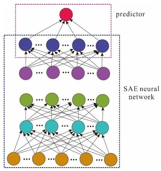
Figure 1.
SAE neural network prediction model.
We suppose that the SAE consists of n AEs, and bb(1) and W(1) are the biases and weights between the import and the hidden layer. Further, bb(2) and W(2) are the biases and weights between the hidden and the export layers. , , , and are the biases and weights of the kth AE, and the corresponding values are bb(1), W(1), bb(2), and W(2). The coding process of each AE layer are realized in sequence from beginning to end according to Equations (4) and (5), written as
The decoding process of each layer of AE was implemented in sequence from back to front as
where aa(l) is the activation value of the SAE at the l level, and aa(n) is the activation value of the deepest hidden layer.
The training process of the SAE is introduced as given in the following:
- (1)
- Greedy training layer by layer without supervision
We have employed the greedy training layer by layer without supervision means, proposed by Hinton (2006) [25], to obtain the parameters of the SAE. The specific process is given as follows:
(1) We import the initial data x(k), train the first SAE, import the import data into the SAE, and obtain the first-order characteristics of the import data, as shown in Figure 2.
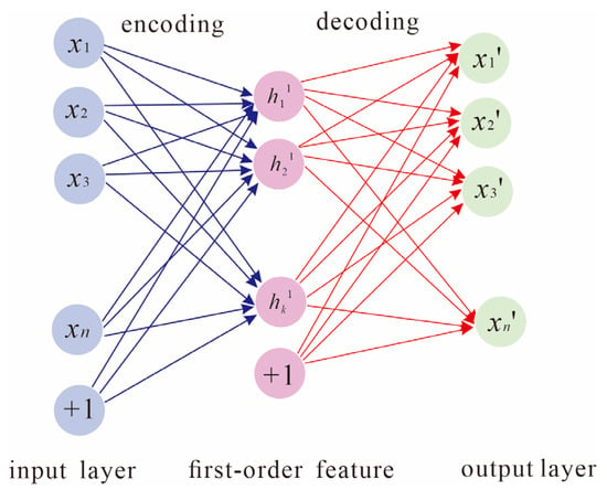
Figure 2.
Training framework diagram of the first AE.
(2) The first-order feature obtained in step (1) is utilized as the import of the second SAE to train the same. We import the first-order feature into the second SAE to obtain the second-order feature of the import data, as shown in Figure 3. In Figure 3, q < k, i.e., the dimension of the second-order feature vector is smaller than the dimension of the first-order feature vector.
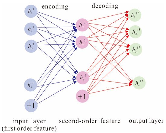
Figure 3.
Training framework diagram of the second AE.
(3) We repeat steps (1) and (2) until the last SAE has been trained and the highest order feature vector is obtained.
- (2)
- Supervised fine adjustment
After completing the greedy training without supervision, the optimal solution of the net parameters of each layer are obtained. However, we need to connect the whole network together and re-train at this instant so that the network parameters of each layer can be improved concomitantly.
First, the pre-training results of the SAE on the parameters of each layer are taken as the initial weight, and then the weights of all layers are re-propagated forward to calculate the error cost function of the whole network. Finally, the gradient descent means is employed to iteratively renew the net parameters to minimize the error cost function value of the whole network, thus completing the training of the whole network. The error cost function expression is given as
where x is the initial import data, and is the mean square error term, which minimizes the reconstruction error. The second item is the weight attenuation item, and is the weight attenuation item coefficient that reduces the amplitude of the weight and avoids the occurrence of over-fitting. h(n) is an important feature of the import data learned by the SAE after multiple nonlinear transformations.
2.3. CHSIP
The concurrent heuristic search iterative process (CHSIP) is conducted for the GPSE in this work and the concrete implementation of CHSIP is shown in Figure 4. For the first iteration in the CHSIP, the starting points are determined by specialized experience, while for the subsequent iterations in the CHSIP, the judging standard of state transition determines the starting points. When the stopping criterion of the CHSIP is satisfied, the process stops. At the same time, the estimation outcomes for unknown variables are acquired. The detailed process is explained in our informed research [26].
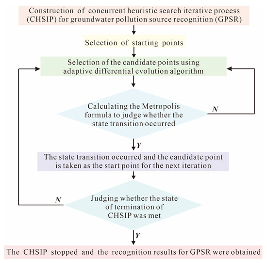
Figure 4.
Concrete implementation of CHSIP in this case study.
3. Application
3.1. Site Profile
We designed a hypothetical case study (Figure 5) to verify the performance of the proposed CHSIP with the SAE substitute. The study area is selected as a rectangle of 1600 m × 1200 m. The hypothesis of the research domain is given as follows: the BC and DA are the confining borders, and AB and CD are the given head borders. For this hypothetical case, 24 months of simulating time is averaged and separated into eight periods and the study domain is separated into three zones regarding the permeability coefficient. The discharge strength in the first three intervals, the permeability coefficient in the three zones, and the longitudinal and transverse dispersity are all unknown variables in this case study. The permeability coefficient is an important hydrogeological parameter that can reflect the permeability of the aquifer. The greater permeability coefficient, the greater the permeability of the aquifer. Dispersity is an important index to characterize the hydrodynamic dispersion strength of groundwater pollution, which has a significant impact on groundwater pollution transport. Table 1 demonstrates the truth values of the unknown discharge strengths, permeability coefficients and dispersity according to professional knowledge and the physical characteristics of the parameters themselves. For the hypothetical case, the monitoring data of groundwater pollution at the three monitoring wells are not observed in the eight periods but are obtained by operating the mathematical simulator based on the truth values of the unknown variables (Table 2 and Figure 6). In the following study of the GPSE, we treat these variables as unknown and estimate their true values through a concurrent heuristic search iterative process with the SAE substitute.
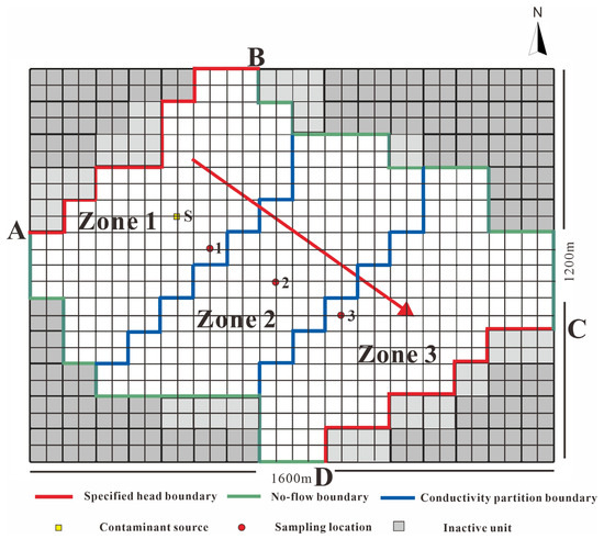
Figure 5.
Basic overview of the research domain. The red arrow represents groundwater flow. Points 1, 2 and 3 represent monitoring wells 1, 2, and 3.

Table 1.
Truth values of discharge strengths, permeability coefficients and dispersity. P1, P2, and P3 denote discharge strength of the pollution source in the first three intervals, respectively. K1, K2, and K3 denote permeability coefficients in zones 1~3. L and T represent longitudinal and transverse dispersity.

Table 2.
Concentration monitoring data of groundwater pollution at three monitoring wells.
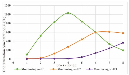
Figure 6.
Monitoring data of groundwater pollution at three monitoring wells. Different colored lines represent different monitoring wells.
3.2. Operation of Simulator
Firstly, we analyze the case study and generalize the basic hydrogeological situation of the case. Then, we build a hydrogeological conceptual model to describe the case study. Based on the hydrogeological conceptual model, the mathematical simulation of the groundwater pollution (including groundwater flow model and solute transport model) is established. For the partial differential equation, one can refer to Equations (1)–(3). In this work, the MODFLOW and MT3DMS computing modules in GMS software are employed to solve the groundwater flow model and the solute transport model. The values of the pollution source and the aquifer parameters are input into the simulator, and the output values of the simulator (i.e., the groundwater pollution concentrations) are obtained by solving the simulation model.
3.3. Establishment of Substitute
3.3.1. Acquiring of Training and Testing Samples
The import vector of the simulator or the substitute for each monitoring well includes eight unknown variables (three discharge strengths of the pollution source, three permeability coefficients and the longitudinal and transverse dispersity), and the exports of the simulator or the substitute are the groundwater pollution concentrations at the end of each period. Initially, we employed the Latin hypercube sampling method to acquire 400 sets of import data for the training samples and 100 sets of import data for the testing samples for eight unknown variables in their feasible regions. Afterwards, we ran the groundwater pollution simulator with the 500 sets of input data to obtain the corresponding groundwater pollution concentrations as export data, and consequently, 500 sets of import-export samples for eight unknown variables were obtained. Particularly for the 500 sets of import–export samples, the first 400 sets are used for establishing the substitute and the remaining 100 sets are used for testing the approach accuracy of the substitute for the simulation. The 400 sets of import–export training samples are employed to build the GP and the SAE substitute for the three monitoring wells and six substitutes are set up in total. Then, the 100 sets of the import data of testing samples are separately imported into the GP and SAE substitutes to obtain the export values. Finally, the export values of the GP and SAE substitutes are compared with those of the simulator. By comparing the proximity of the export values from the substitute and simulator, the approach accuracy of the substitute for the simulation is tested.
3.3.2. Establishment of GP Substitute
First, the import–export data are normalized, and then the codes of GP substitute are written in MATLAB software (Version 2012a) according to the principle of the GP method. Training samples and testing samples are used to train and validate the GP substitute, respectively. The undetermined parameters of the GP substitute [27] are optimized, and the corresponding parameters are demonstrated in Table 3.

Table 3.
Undetermined parameters of GP substitute.
3.3.3. Establishment of SAE Substitute
The SAE substitute of the numerical simulator of groundwater pollution has been established by employing the SAE neural network method.
The specific process is given as follows:
(1) Data normalization
Normalize the import data.
(2) Training of the SAE substitute
Use the training samples to train the SAE substitute.
The feature learning of the training samples is carried out to obtain the higher-order feature representation of the reconstructed data. The training effect of the SAE neural network is optimized after greedy training layer by layer without supervision and a supervised fine adjustment.
Problems of over-fitting and under-fitting easily occur in the training process of the SAE neural network. Over-fitting occurs if the network structure is too complex. However, if the training data were too complex and the network structure was too simple, under-fitting occurs. This paper discusses the influence of the setting of the SAE neural network, with respect to the above problems, on the results of the network training.
When the training data are fixed, more neurons in the network implies a more complex network structure and a more likely occurrence of the over-fitting phenomenon. Therefore, fewer layers of the network RE are better under the condition of meeting the precision requirement. In this paper, an SAE with two hidden layers was selected for training.
Previous studies [9] have shown that the quantity of neurons in a hidden layer should approximate the amount of import and export layers to prevent the occurrence of over-fitting. The number of import layers in this paper is eight, and the number of export layers is eight. If the neuron numbers in the two hidden layers are L1 and L2, respectively, then . Then, the training data are employed to train the SAE. We change the quantity of neurons (i.e., L1 and L2) in the two hidden layers and calculate the error cost function, respectively. The calculation results are displayed in Figure 7.
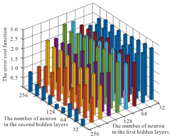
Figure 7.
Impact of the quantity of the hidden layer neurons on the neural net training results. Different colored boxes represent different quantities of neurons in the first and second hidden layers.
Figure 7 indicates that the quantity of neurons in a hidden layer of the AE has varying degrees of impact on the network training results. When the L2 value remains unchanged, the error cost changes with the change in L1. Further, the change is significant, indicating that the value of L1 has a greater influence on the net training outcomes than L2. When the value of L1 is around 64, the value of the error cost function is the smallest. Similarly, the error cost function value is minimized when L1 remains constant and L2 is around 32. When L1 = 64 and L2 = 32, the error cost function has the smallest value.
After completing the training of the SAE substitute, the import data are imported into the trained SAE substitute to obtain the export data.
(3) Data denormalization processing
Perform denormalization on the export data in step (2).
4. Outcomes and Discussions
4.1. Accuracy of the Substitute
The approach accuracy of the substitute for the mathematical simulator has a tremendous influence on the estimation precision. After testing the precision of the GP and SAE substitutes of three monitoring wells, the substitute with a highest approximate precision is selected as the final substitute of the numerical simulator in the subsequent estimation.
The import of the substitute for each monitoring well includes eight unknown variables. Accordingly, the groundwater pollution concentrations at the end of eight periods form the export data of the substitute, i.e., 100 sets of testing samples include 800 pollution concentration values (export data) overall. Scatter plots of the numerical simulator exports, the GP substitute exports, and the SAE substitute exports are displayed in Figure 8, Figure 9 and Figure 10. Scatters for the SAE substitute is more centrally located around y = x. This demonstrates that the SAE substitute has higher approach precision with regards to the mathematical simulation than the GP substitute.
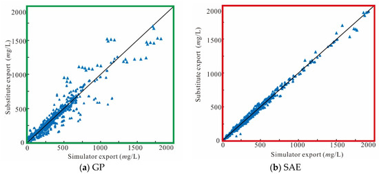
Figure 8.
Fitted regression of substitute exports and simulator exports at monitoring well 1.
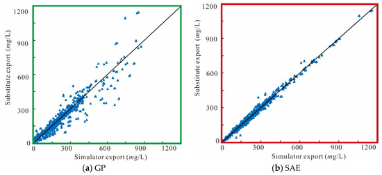
Figure 9.
Fitted regression of substitute exports and simulator exports at monitoring well 2.
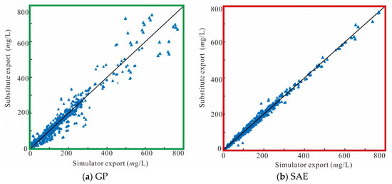
Figure 10.
Fitted regression of substitute exports and simulator exports at monitoring well 3.
Moreover, the above substitutes are compared using four precision evaluation indexes (Table 4 and Figure 11). Smaller values of Average Relative Error, Maximum Relative Error and Root Mean Square Error entail a higher approach accuracy of the substitute compared to the simulator. The closer the Association Coefficient is to one, the higher the approach accuracy of the substitute. The above indicators in Table 4 reveal that the SAE substitute has a higher approach accuracy to the simulator. Hence, the SAE substitute was selected as the final substitute for the simulator in the subsequent estimation.

Table 4.
Precision evaluation indexes of two substitutes of three monitoring wells. Index I denotes Association Coefficient. Index II denotes Maximum Relative Error. Index III denotes Root Mean Square Error. Index IV denotes Average Relative Error.
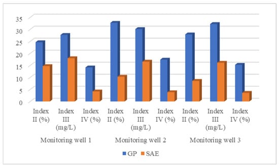
Figure 11.
Four precision evaluation indexes of two substitutes for three monitoring wells. The blue box denotes the GP substitute, and the orange box denotes the SAE substitute. The first three sets of indexes refer to monitoring well 1, the middle three refer to monitoring well 2, and the last three refer to monitoring well 3.
4.2. Estimation Outcomes
The group individual number is set to five in the adaptive differential evolution algorithm for the CHSIP, and the number of iterations in the CHSIP is 20,000. Overall, the operation time of the mathematical simulation is 100,000 iterations. Running the mathematical simulation takes 20 s, whereas calculating the SAE substitute takes only 0.6 s, which greatly reduces the calculated load. To judge whether the convergence of the CHSIP occurs, we choose the scale reduction score as the convergence criterion in this work [28].
The scale reduction score curve is plotted on the MATLAB platform (Figure 12). The scale reduction score is less than 1.2 after 15,000 iterations in the CHSIP. In other words, the CHSIP converged at 15,000 iterations. We choose the ultimate 1000 iterations with 5000 values as the best representative samples for the unknown variables. We implemented a statistical analysis of each unknown variable on MATLAB. We input the 5000 values of unknown variables into the MATLAB platform for data analysis, including point and interval estimations. We draw the posterior probability density function (PPDF) curve of each unknown variable (Figure 13) using the curve plotting function in MATLAB. The interval estimation can be gained based on the PPDF curves. In terms of point estimation, we choose the value with the maximum PPDF. The outcomes show that the point estimation has a high approach accuracy to the truth values. Figure 14 and Table 5 display the relative errors between the truth values and point estimations. The outcome proves that the CHSIP with the SAE substitute can effectively and accurately estimate the groundwater pollution source and aquifer parameters.
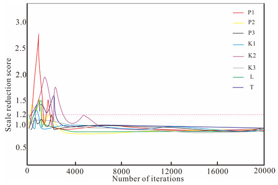
Figure 12.
Curve plotting of scale reduction score. Different colored lines represent scale reduction scores for different unknown variables.

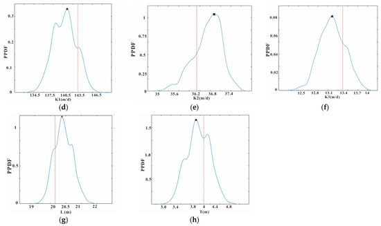
Figure 13.
PPDF curve of unknown variables (a–h). The black cross represents the point estimation. The blue line represents the PPDF curve. The vertical dotted red line represents the truth value of the unknown variable.
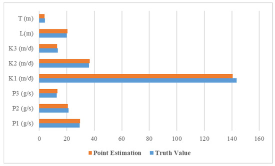
Figure 14.
Truth value and point estimation of unknown variables. The blue box represents the truth value, and the orange box represents the point estimation of the unknown variable.

Table 5.
Relative error between truth value and point estimation of unknown variable.
5. Conclusions
We employed the CHSIP for estimating the groundwater pollution source and aquifer parameters. The repetitive running of a mathematical simulator effectuated a large calculated load during the CHSIP. Building a substitute for the mathematical simulator can effectively decrease the calculation pathways. However, there is a complicated nonlinear correlativity between the import and export of the mathematical simulation. This leads to the poor approach accuracy of the substitute compared to the mathematical simulator using shallow learning methods. Therefore, we first established a stacked autoencoder substitute using the deep learning method to enhance the approximation accuracy of the substitute for the mathematical simulator. The CHSIP is implemented for estimating, and the estimation results are acquired when the CHSIP is terminated. Our approaches are based on a hypothetical case, which show that the CHSIP is helpful for estimating the groundwater pollution source and aquifer parameters. Further, the stacked autoencoder method can effectively enhance the approach accuracy of the substitute to the mathematical simulator.
Author Contributions
All authors contributed to the study’s conception and design. The conceptualization of the mathematical simulator was conducted by J.Z. Methodology application was conducted by J.G. Software operation was conducted by G.L. The validation of the substitute was conducted by W.L. Writing—original draft was conducted by H.W. and writing—the revised version of paper was conducted by H.L. All authors approved the final manuscript. All authors have read and agreed to the published version of the manuscript.
Funding
This research was funded by the National Natural Science Foundation of China (No. 41972252).
Data Availability Statement
To protect the rights of authors and avoid plagiarism, and for reasons of data privacy, the data in this paper cannot be shared openly.
Conflicts of Interest
All authors state that they have no known competing financial interests in this article.
References
- Guo, J.; Lu, W.; Yang, Q.; Miao, T. The application of 0–1 mixed integer nonlinear programming optimization model based on a surrogate model to identify the groundwater pollution source. J. Contam. Hydrol. 2019, 220, 18–25. [Google Scholar] [CrossRef] [PubMed]
- Lapworth, D.J.; Baran, N.; Stuart, M.E.; Ward, R.S. Emerging organic contaminants in groundwater: A review of sources, fate and occurrence. Environ. Pollut. 2012, 163, 287–303. [Google Scholar] [CrossRef] [PubMed]
- Yao, Y.; Yang, F.; Suuberg, E.M.; Provoost, J.; Liu, W. Estimation of contaminant subslab concentration in petroleum vapor intrusion. J. Hazard. Mater. 2014, 279, 336–347. [Google Scholar] [CrossRef] [PubMed][Green Version]
- Zanini, A.; D’Oria, M.; Tanda, M.G.; Woodbury, A.D. Coupling empirical Bayes and Akaike’s Bayesian information criterion to estimate aquifer transmissivity fields. Math. Geosci. 2020, 52, 425–441. [Google Scholar] [CrossRef]
- Mirghani, B.Y.; Zechman, E.M.; Ranjithan, R.S.; Mahinthakumar, G. Enhanced Simulation-Optimization Approach Using Surrogate Modeling for Solving Inverse Problems. Environ. Forens. 2012, 13, 348–363. [Google Scholar] [CrossRef]
- Shen, C.P. A Transdisciplinary Review of Deep Learning Research and Its Relevance for Water Resources Scientists. Water Resour. Res. 2018, 54, 8558–8593. [Google Scholar] [CrossRef]
- Mirarabi, A.; Nassery, H.R.; Nakhaei, M.; Adamowski, J.; Akbarzadeh, A.H.; Alijani, F. Evaluation of data-driven models (SVR and ANN) for groundwater-level prediction in confined and unconfined systems. Environ. Geol. 2019, 78, 489.1–489.15. [Google Scholar] [CrossRef]
- Zanini, A.; Tanda, M.G.; Woodbury, A.D. Identification of transmissivity fields using a Bayesian strategy and perturbative approach. Adv. Water Resour. 2017, 108, 69–82. [Google Scholar] [CrossRef]
- Asher, M.J.; Croke, B.F.W.; Jakeman, A.J.; Peeters, L.J.M. A review of surrogate models and their application to groundwater modeling. Water Resour. Res. 2015, 51, 5957–5973. [Google Scholar] [CrossRef]
- Prakash, O.; Datta, B. Sequential optimal monitoring network design and iterative spatial estimation of pollutant concentration for identification of unknown groundwater pollution source locations. Environ. Monit. Assess. 2012, 185, 5611–5626. [Google Scholar] [CrossRef]
- Zhao, Y.; Qu, R.; Xing, Z.; Lu, W. Identifying groundwater contaminant sources based on a KELM surrogate model together with four heuristic optimization algorithms Adv. Water Resour. 2020, 138, 103540. [Google Scholar] [CrossRef]
- Lu, W.; Wang, H.; Li, J. Parallel heuristic search strategy based on a Bayesian approach for simultaneous recognition of contaminant sources and aquifer parameters at DNAPL-contaminated sites. Environ. Sci. Pollut. Res. 2020, 27, 37134–37148. [Google Scholar] [CrossRef] [PubMed]
- Xing, Z.; Qu, R.; Zhao, Y.; Fu, Q.; Ji, Y.; Lu, W. Identifying the Release History of a Groundwater Contaminant Source Based on an Ensemble Surrogate Model. J. Hydrol. 2019, 572, 501–516. [Google Scholar] [CrossRef]
- Zhao, Y.; Lu, W.; Xiao, C. A Kriging surrogate model coupled in simulation-optimization approach for identifying release history of groundwater sources. J. Contam. Hydrol. 2016, 185–186, 51–60. [Google Scholar] [CrossRef]
- Han, Z.; Lu, W.; Fan, Y.; Lin, J.; Yuan, Q. A surrogate-based simulation-optimization approach for coastal aquifer management. Water Supply 2020, 20, 3404–3418. [Google Scholar] [CrossRef]
- Matott, L.S.; Rabideau, A.J. Calibration of complex subsurface reaction models using a surrogate-model approach. Adv. Water Resour. 2008, 31, 1697–1707. [Google Scholar] [CrossRef]
- Zanini, A.; Woodbury, A.D. Contaminant source reconstruction by empirical Bayes and Akaike’s Bayesian Information Criterion. J. Contam. Hydrol. 2016, 185–186, 74–86. [Google Scholar] [CrossRef]
- Jin, J.; Zhang, C.; Feng, F.; Na, W.C.; Ma, J.G.; Zhang, Q.J. Deep Neural Network Technique for High-Dimensional Microwave Modeling and Applications to Parameter Extraction of Microwave Filters. IEEE Trans. Microw. Theory 2019, 67, 4140–4155. [Google Scholar] [CrossRef]
- Zhao, Y.; Lu, W.; An, Y. Surrogate model-based simulation-optimization approach for groundwater source identification problems. Environ. Forensics 2015, 16, 296–303. [Google Scholar] [CrossRef]
- Zhou, C.; Zhou, J.; Cai, Y.U.; Zhao, W.; Pan, R. Multi-channel sliced deep RCNN with residual network for text classification. Chin. J. Electron. 2020, 29, 880–886. [Google Scholar] [CrossRef]
- Popa, C.A. Complex-Valued Deep Belief Networks. In Advances in Neural Networks–ISNN 2018: 15th International Symposium on Neural Networks, ISNN 2018, Minsk, Belarus, 25–28 June 2018; Springer: Cham, Switzerland, 2018. [Google Scholar]
- Wang, S.H.; Phillips, P.; Sui, Y.; Liu, B.; Yang, M.; Cheng, H. Classification of Alzheimer’s disease based on Eight-layer convolutional neural network with leaky rectified linear unit and max pooling. J. Med. Syst 2018, 42, 85. [Google Scholar] [CrossRef] [PubMed]
- Hinton, G.E.; Osindero, S.; Teh, Y.W. A fast learning algorithm for deep belief nets. Neural Comput. 2014, 18, 1527–1554. [Google Scholar] [CrossRef] [PubMed]
- Malihi, L.; Malihi, R. Single stuck-at-faults detection using test generation vector and deep stacked-sparse-autoencoder. SN Appl. Sci. 2020, 2, 1715. [Google Scholar] [CrossRef]
- Hinton, G.E.; Salakhutdinov, R. Reducing the dimensionality of data with neural networks. Science 2006, 313, 504–507. [Google Scholar] [CrossRef] [PubMed]
- Wang, H.; Lu, W.; Chang, Z. An iterative updating heuristic search strategy for groundwater contamination source identification based on an ACPSO-ELM surrogate system. Stoch. Env. Res. Risk Assess. 2021, 35, 2153–2172. [Google Scholar] [CrossRef]
- Wang, H.; Lu, W. Groundwater contamination source-sink analysis based on random statistical method for a practical case. Stoch. Env. Res. Risk Assess. 2022, 36, 4157–4174. [Google Scholar] [CrossRef]
- Wang, H.; Lu, W.; Li, J. Groundwater contaminant source characterization with simulator parameter estimation utilizing a heuristic search strategy based on the stochastic-simulation statistic method. J. Contam. Hydrol. 2020, 234, 103681. [Google Scholar] [CrossRef]
Disclaimer/Publisher’s Note: The statements, opinions and data contained in all publications are solely those of the individual author(s) and contributor(s) and not of MDPI and/or the editor(s). MDPI and/or the editor(s) disclaim responsibility for any injury to people or property resulting from any ideas, methods, instructions or products referred to in the content. |
© 2024 by the authors. Licensee MDPI, Basel, Switzerland. This article is an open access article distributed under the terms and conditions of the Creative Commons Attribution (CC BY) license (https://creativecommons.org/licenses/by/4.0/).