Groundwater LNAPL Contamination Source Identification Based on Stacking Ensemble Surrogate Model

Abstract

Groundwater LNAPL (Light Non-Aqueous Phase Liquid) contamination source identification (GLCSI) is essential for effective remediation and risk assessment. Addressing the GLCSI problem often involves numerous repetitive forward simulations, which are computationally expensive and time-consuming. Establishing a surrogate model for the simulation model is an effective way to overcome this challenge. However, how to obtain high-quality samples for training the surrogate model and which method should be used to develop the surrogate model with higher accuracy remain important questions to explore. To this end, this paper innovatively adopted the quasi-Monte Carlo (QMC) method to sample from the prior space of unknown variables. Then, this paper established a variety of individual machine learning surrogate models, respectively, and screened three with higher training accuracy among them as the base-learning models (BLMs). The Stacking ensemble framework was utilized to integrate the three BLMs to establish the ensemble surrogate model for the groundwater LNAPL multiphase flow numerical simulation model. Finally, a hypothetical case of groundwater LNAPL contamination was designed. After evaluating the accuracy of the Stacking ensemble surrogate model, the differential evolution Markov chain (DE-MC) algorithm was applied to jointly identify information on groundwater LNAPL contamination source and key hydrogeological parameters. The results of this study demonstrated the following: (1) Employing the QMC method to sample from the prior space resulted in more uniformly distributed and representative samples, which improved the quality of the training data. (2) The developed Stacking ensemble surrogate model had a higher accuracy than any individual surrogate model, with an average R² of 0.995, and reduced the computational burden by 99.56% compared to the inversion process based on the simulation model. (3) The application of the DE-MC algorithm effectively solved the GLCSI problem, and the mean relative error of the identification results of unknown variables was less than 5%.

1. Introduction

Petroleum-based organic contaminants, such as Light Non-Aqueous Phase Liquids (LNAPLs), can pose significant threats to groundwater quality. These contaminants can infiltrate groundwater through the vadose zone, primarily due to accidental releases during production, transportation, or storage [1,2,3]. Due to their lower density than water, LNAPLs tend to accumulate at the water table, forming a persistent source of contamination. The continuous dissolution of contaminants from these LNAPL pools can pose long-term risks to groundwater safety [4]. To effectively remediate LNAPL contamination, it is essential to identify the characteristics of the contamination source, including its location, release history, and key hydrogeological parameters [5]. While existing research has primarily focused on source identification for conservative contaminant transport processes, investigations into the identification of multiphase flow processes associated with LNAPL contamination remain relatively limited. Therefore, exploring solutions for identifying LNAPL sources in groundwater holds significant theoretical and practical implications for groundwater pollution prevention and control.

Traditional methods for groundwater LNAPL contamination source identification (GLCSI), such as simulation optimization [6,7], Bayesian-based stochastic approaches [8,9], and data assimilation techniques [10,11], rely on computationally intensive iterative search processes that require repeated forward simulations. This often leads to prohibitive computational costs. Surrogate models, also known as proxy models, provide an approximation of complex simulation models, capturing their essential features and mimicking their behavior. An effective surrogate model should produce outputs closely resembling those of the simulation model for the same input while offering a significantly lower computational cost. Therefore, by establishing a surrogate model for the simulation model, we can replace the simulation model with the surrogate model during the iterative search process, significantly improving the efficiency of source identification and effectively mitigating the computational burden [12,13].

Surrogate models, commonly used in hydrology, are predominantly data-driven [14]. These models function without considering the underlying physical processes of the system, focusing solely on extracting data features to establish input–output relationships. With advancements in artificial intelligence and big data technologies, numerous studies have applied machine learning-based data-driven surrogate models for GLCSI [15,16]. These models are categorized into two main approaches: shallow learning and deep learning. Zhao et al. used a kernel-based extreme learning machine (KELM) as a surrogate for the simulation model, coupled with the optimization model, to reversely determine the source’s contaminant concentration range [17]. In addition, widely used surrogate models based on shallow learning include Kriging (KRG) [18] and Support Vector Regression (SVR) [19]. These surrogate models, each built using a specific method, were referred to as individual surrogate models. Generally, for simulation models with complex mapping relationships, deep learning-based individual surrogate models exhibited stronger learning capabilities compared to those based on shallow learning. Wang et al. applied the deep belief neural network (DBN) surrogate model and the deep residual neural network (DRN) to develop a deep learning combined surrogate model, which further enhanced the approximation precision to the numerical simulation model [20]. Deep learning methods, such as Generative Adversarial Networks (GANs) [21] and Long Short-Term Memory Networks (LSTMs) [22] were also widely used.

As real-world problems become more complex, characterized by higher dimensions of unknown variables and increased system non-linearity, individual surrogate models built for the simulation model tend to perform unevenly and with generally lower accuracy. To overcome this limitation, researchers have explored ensemble learning-based surrogate models. These ensemble models combine multiple individual models, known as base-learning models (BLMs), to approximate complex simulation models. Effective combinations of BLMs can lead to highly accurate and robust ensemble surrogate models. Based on the type of BLM used, ensemble methods can be categorized as homogeneous ensembles and heterogeneous ensembles [23]. Homogeneous ensembles employ the same type of BLM but train them with different datasets. They can be further classified into serial ensemble methods, such as Boosting, and parallel ensemble methods, such as Bagging. Both Bagging and Boosting methods have been successfully applied in hydrological process modeling [24,25]. Heterogeneous ensembles, on the other hand, utilize different BLMs, with model averaging (MA) and Stacking being prominent examples. MA utilizes optimization methods or heuristics to minimize the error between the simulation model output and the ensemble surrogate model output, thereby determining optimal weights for each BLM. During prediction, the outputs of the BLM were combined according to these optimized weights, resulting in the ensemble surrogate model’s output [26]. MA has been widely applied in building surrogate models for simulation models used in GLCSI problems [27,28,29]. The Stacking ensemble method combines different BLMs, effectively leveraging their individual strengths to achieve optimal performance. Compared with the homogeneous integration methods of Bagging and Boosting, the Stacking integration method can better utilize the unique advantages of each BLM and make full use of their strengths to complement their weaknesses. Compared with the MA method, the Stacking integration method is not a simple linear weighting when combining each BLM, but combines them through another BLM (called meta-learning model, MLM), which is a kind of non-linear combination [30,31]. The application of Stacking to build surrogate models for the simulation model of multiphase flow in GLCSI has been rarely reported and remains to be explored. This study compared the performance of various BLMs, including KRG, KELM, Random Forest (RF), Multilayer Perceptron (MLP), and DBN, and resulted in the selection of RF, DBN, and MLP as the BLMs, with MLP as the MLM to propose a Stacking ensemble model for the multiphase flow numerical simulation model.

The choice of BLM and ensemble methods is not the sole factor determining the effectiveness of surrogate models. The quality of the training samples used to build these models also plays a significant role [32,33]. While ideal samples would be drawn from the posterior space of the unknown variables, this is often unrealistic in practice. Given the initial lack of knowledge about these variables, a practical approach involves distributing samples uniformly within their prior space. Common methods for obtaining samples of unknown variables include orthogonal experimental design [34], Monte Carlo random sampling [35], and Latin hypercube sampling [36]. This study employed a quasi-Monte Carlo (QMC) method to extract samples from the prior space of unknown variables. This method strategically selects locations for pseudo-random numbers, ensuring that the resulting samples are evenly spaced within the random space, which allows for the acquisition of maximum information about variable characteristics with the least number of samples.

A hypothetical LNAPL contamination case was designed to evaluate the effectiveness of the proposed methodology. The unknown variables, in this case, included source characteristics (longitudinal and transverse coordinates, initial and final release times, and release intensity) and hydrogeological parameters (longitudinal and transverse hydrodynamic dispersion coefficients, porosity, and permeability). To accurately model the LNAPL contamination site, the permeability was represented as a random field controlled by 11 random numbers using Karhunen–Loève (KL) expansion techniques. Therefore, the case involved 19 unknown variables. The surrogate model for the LNAPL contamination groundwater multiphase flow solute transport numerical simulation model was constructed using the proposed QMC sampling method and the Stacking ensemble approach. After validating the accuracy of the surrogate model, a differential evolution Markov chain (DE-MC) method was employed to identify the 19-dimensional variables. In a word, this study is a new attempt to adopt the Stacking ensemble framework with QMC sampling to establish the ensemble surrogate for the groundwater LNAPL contamination groundwater multiphase flow solute transport numerical simulation model. The outcomes present a new perspective on inversion techniques, enrich the theoretical underpinnings of GLCSI, and offer technical support for practical applications.

This paper is organized as follows: The simulation model, some basic theories, and the proposed algorithm are presented in Section 2. In Section 3, the performance of the proposed algorithm is evaluated by using a case study. Finally, the results and discussions of this study are presented in Section 4.

2. Methods

2.1. Simulation Model for Multiphase Flow

According to the principle of conservation of mass, the mass continuity of a component in a multiphase flow per unit time and per unit pore volume can be expressed as follows [37,38]:

$${\displaystyle \frac{\partial }{\partial t}}\left(\varphi {\tilde{C}}_k{\rho }_k\right)+\overrightarrow{\nabla }\cdot \left[{\displaystyle \sum _{l=1}^{n_p}{\rho }_k\left(C_{kl}{\overrightarrow{u}}_l-{\overrightarrow{\tilde{D}}}_{kl}\right)}\right]=R_k$$

(1)

where the total volume of component $k$ per unit pore volume is the sum of its components in all phases:

$${\tilde{C}}_k=\left(1-{\displaystyle \sum _{k=1}^{n_{\mathrm{cv}}}{\widehat{C}}_k}\right){\displaystyle \sum _{l=1}^{n_{\mathrm{p}}}{S}_l{C}_{kl}}+{\widehat{C}}_k\hspace{1em}\mathrm{for}k=1,\cdots ,n_{\mathrm{cv}}$$

(2)

where $k$ represents a specific component; $n_{\mathrm{cv}}$ represents the total number of components; ${\widehat{C}}_k$ represents the adsorption concentration of component $k$; $l$ represents a specific phase; $n_{\mathrm{p}}$ represents the total number of phases (including the aqueous, oil, and gas phases); $S_l$ represents the saturation of phase $l$; the sum of saturations of all phases is 1; $C_{kl}$ represents the concentration of component $k$ in phase $l$; ${\rho }_k$ represents the density of the component; and $R_k$ represents the source/sink term for component $k$.

According to Fick’s law, the dispersive flux ${\overrightarrow{\tilde{D}}}_{kl}$ of component $k$ in phase $l$ can be expressed as follows:

$${\overrightarrow{\tilde{D}}}_{kl,x}=\varphi S_l{\overrightarrow{\overrightarrow{K}}}_{kl}\cdot \overrightarrow{\nabla }{C}_{kl}$$

(3)

where the dispersion coefficient tensor ${\overrightarrow{\overrightarrow{K}}}_{kl}$ including molecular diffusion $D_{kl}$ is calculated as follows:

$${\overrightarrow{\overrightarrow{K}}}_{kl\mathrm{ij}}={\displaystyle \frac{D_{kl}}{\tau }}{\delta }_{\mathrm{ij}}+{\displaystyle \frac{{\alpha }_{Tl}}{\varphi S_l}}|{\overrightarrow{\mathrm{u}}}_l|{\delta }_{\mathrm{ij}}+{\displaystyle \frac{({\alpha }_{Ll}-{\alpha }_{Tl})}{\varphi S_l}}{\displaystyle \frac{{\mathrm{u}}_{l\mathrm{i}}{\mathrm{u}}_{l\mathrm{j}}}{|{\overrightarrow{\mathrm{u}}}_l|}}$$

(4)

where ${\alpha }_{Ll}$ and ${\alpha }_{Tl}$ represent the longitudinal and transverse dispersivities of phase $l$, respectively, $\tau$ is the pore tortuosity, which has a value greater than 1; ${\mathrm{u}}_{l\mathrm{i}}$ and ${\mathrm{u}}_{l\mathrm{j}}$ are the components of the Darcy flux of phase $l$ in the $\mathrm{i}$ and $\mathrm{j}$ directions, respectively; and ${\delta }_{\mathrm{ij}}$ represents the Kronecker delta function. The flux in each phase is calculated according to Darcy’s law as follows:

$${\overrightarrow{\mathrm{u}}}_l=-{\displaystyle \frac{{\mathrm{k}}_{\mathit{rl}}\overrightarrow{\overrightarrow{\mathrm{k}}}}{{\mathrm{u}}_l}}\cdot \left(\overrightarrow{\nabla }{\mathrm{P}}_l-{\gamma }_l\overrightarrow{\nabla }\mathrm{h}\right)$$

(5)

where ${\mathrm{k}}_{rl}$ represents the relative permeability of phase $l$; $\overrightarrow{\overrightarrow{\mathrm{k}}}$ represents the intrinsic permeability tensor; $\mathrm{h}$ represents the depth in the vertical direction; ${\mathrm{u}}_l$ represents the viscosity of the phase; ${\mathrm{P}}_l$ represents the pressure of phase $l$; and ${\gamma }_l$ represents the specific gravity of phase $l$.

The LNAPL contamination groundwater multiphase flow solute transport numerical simulation model was formulated by combining the partial differential in Equation (1) with initial and boundary conditions. This model was solved using the UTCHEM 9.82 software developed by the University of Texas. The specific initial and boundary conditions are provided in Section 3.1.

2.2. Quasi-Monte Carlo Sampling

Sampling techniques aim to approximate integrals by drawing random samples of variables from known probability distributions. Monte Carlo (MC) methods, which rely on pseudorandom numbers, are widely used for this purpose. Since the 1960s, research has focused on using highly uniform sequences to approximate integrals [39]. These highly uniform sequences are known as quasi-Monte Carlo point sets [40]. Replacing pseudorandom numbers with quasi-Monte Carlo point sets in MC simulations is known as the quasi-Monte Carlo (QMC) method. The objective of QMC methods is to optimize MC methods by deterministically choosing the locations of pseudorandom numbers used to generate sample points. This ensures that sample points are evenly spaced within the random space, maximizing the information extracted about the variable characteristics using a minimal number of samples. This paper employed the Sobol sequence [41] from the theory of number-theoretic nets to generate QMC point sets. In practical applications, the Sobol sequence was generated using the sobolset package in MATLAB (R2021a).

QMC sampling involves the following steps:

(1)

Generate a Sobol sequence $U_n=\left\{u_i:i=1,2,\cdots ,n\right\}$ that fills the $d$-dimensional space ${\left(0,1\right)}^d$, where $d$ is the dimension of the unknown variables and $n$ is the number of samples drawn.

(2)

Apply a random shift to the Sobol sequence. Let $\tau$ be a $d$-dimensional random vector uniformly distributed over ${\left(0,1\right)}^d$. The new sequence ${\tilde{U}}_n=\left\{{\tilde{u}}_i:{\tilde{u}}_i=u_i+\tau \left(mod1\right),i=1,2,\cdots ,n\right\}$, obtained by adding $\tau$ to the Sobol sequence, possesses statistical properties.

(3)

Transform the new sequence ${\tilde{U}}_n$ by applying the prior distribution function of the unknown variables, resulting in $n$ sets of samples representing the unknown variables.

The primary difference between QMC sampling and MC sampling lies in the selection of sample values. Unlike MC methods, the QMC method generates samples by considering previously generated points, ensuring a more even distribution and preventing clustering or gaps in the sample space. This difference is visually illustrated in Figure 1a,b, which depict 100 sample points generated using MC and QMC methods, respectively, within the $d$-dimensional space ${\left(0,1\right)}^2$. Figure 1b shows a more uniform distribution of points across the sampling space, emphasizing the ability of QMC methods to generate more representative samples with the same number of points as MC methods.

2.3. Surrogate Model

2.3.1. Stacking Ensemble Method

Stacking, an ensemble learning method pioneered by Wolpert [42], employs a non-linear approach to combine diverse BLMs. By exploiting the strengths of each BLM, the Stacking ensemble model aims to learn different aspects of the data and achieve superior performance compared to the individual models. This approach involves two primary steps: First, BLMs are trained using the original data to generate meta-data, which encompass the predicted outputs from the BLMs and the corresponding outputs from the original training data. Second, an MLM is trained using the meta-data to make predictions. These two steps work collaboratively to accurately map the input–output relationships found in the original data. Figure 2 provides a visual representation of the conceptual framework of a Stacking ensemble model.

This research evaluated the effectiveness of five BLMs, encompassing two shallow learning models, KRG and KELM, and three deep learning models, MLP, RF, and DBN. These BLMs have been demonstrated as successful surrogate models for groundwater solute transport in previous studies, achieving promising results. This section presents a brief overview of the three deep learning-based BLMs, while comprehensive details about the two shallow learning-based BLMs can be found in References [43,44].

2.3.2. MLP

MLP is a type of feedforward artificial neural network characterized by multiple hidden layers situated between input and output nodes. Except for input nodes, each node is a neuron employing a non-linear activation function. MLP exhibits full connectivity between layers, meaning every neuron in any layer is connected to all neurons in the preceding layer. The strength of these connections is determined by the weight coefficients within the network [45].

Training the MLP model involves two steps: forward computation of the output and backpropagation of errors. Figure 3 illustrates the structure of the MLP model. Firstly, the output is determined based on the given input and current weights. Then, the error function is calculated by subtracting the computed output from the true output. Subsequently, by calculating the partial derivatives of the error function with respect to each weight coefficient, the error is minimized iteratively, thereby training the entire network. The equations for forward computation and backpropagation are presented below:

$$\begin{array}{l}{y}_i^k=f_k\left(u_i^k\right)\hfill \\ u_i^k={\displaystyle \sum _j{w}_{ij}^{k-1}{y}_j^{k-1}}\hfill \end{array}\hspace{1em}k=2,\dots ,m$$

(6)

$$\begin{array}{l}\Delta w_{ij}^{k-1}=-\epsilon d_i^k{y}_j^{k-1}\hfill \\ d_i^m=y_i^m\left(1-y_i^m\right)\left(y_i^m-y_{si}\right)\hfill \\ d_i^k=y_i^k\left(1-y_i^k\right){\displaystyle \sum _l{d}_l^{k+1}{w}_{li}^k}\hspace{1em}k=m-1,\dots ,2\hfill \end{array}$$

(7)

where $y_i^k$ represents the output value of the i-th neuron in the k-th layer. The input–output relationship (function) of the k-th hidden layer is denoted by $f_k$; $u_i^k$ represents the sum of inputs to the i-th neuron in the k-th layer; and $w_{ij}^k$ represents the combined weight between the j-th neuron in the (k−1)-th layer and the i-th neuron in the k-th layer.

2.3.3. RF

RF is an ensemble machine learning method introduced by Breiman [46] for overcoming the overfitting and instability issues associated with individual decision trees. The fundamental principle involves constructing multiple independent decision trees based on random subsets of the initial training dataset. While each tree may exhibit favorable prediction results, they can potentially overfit certain portions of the data. By constructing a large number of independent decision trees and averaging their results as the final simulated outcome, overfitting is mitigated, resulting in enhanced robustness. RF’s randomness manifests in two aspects: firstly, the training set used to construct each decision tree is a random subset of the initial training set; secondly, the features selected for splitting nodes in each decision tree are also a random subset of all features. These two aspects ensure that each pair of decision trees within the constructed RF model is distinct. This study employed the TreeBagger function in MATLAB (R2021a) to construct the Random Forest model. Figure 4 illustrates the structural diagram of the RF model.

2.3.4. DBN

DBN belongs to a kind of artificial intelligence method with deep learning capabilities, which has gained widespread adoption across various research domains since its inception in 2006 [47]. The overall structure of DBN comprises multiple stacked Restricted Boltzmann Machines (RBMs) coupled with a top-level algorithm. RBMs primarily function to extract features from the input data in a layer-wise manner, while the top-level algorithm calculates the final output value of the network.

The DBN model training process typically involves two main stages: unsupervised learning and supervised learning. Firstly, unsupervised learning is performed by training the stacked RBMs in a bottom-up layer-wise manner, aiming to preserve significant feature vectors of the input data as much as possible during the layer-wise mapping computation. Subsequently, supervised learning is employed, utilizing the backpropagation algorithm to fine-tune the relevant parameters of the DBN model. This fine-tuning seeks to establish a non-linear mapping relationship between input and output data, thereby enabling regression prediction capabilities. Figure 5 illustrates the structural diagram of the DBN model.

2.4. Inversion Method

2.4.1. Overview of Bayesian Theory

For a groundwater system model, the relationship between the observation data and input variables can be represented as $Y=f\left(X\right)+\epsilon$, where $f(\cdot )$ denotes the groundwater system simulation model, $X=\left\{x_1,\cdots ,x_d\right\}$ is a vector of $d$ unknown variables, $Y=\left\{y_1,\cdots ,y_n\right\}$ represents the system observation outputs, and $\epsilon =\left\{{\epsilon }_1,\cdots ,{\epsilon }_n\right\}$ is the observation error vector. The GLCSI using Bayesian statistical inference aims to achieve a probabilistic description of the unknown variables $X$ given the observed data $Y$, which means solving the conditional probability $p\left(X|Y\right)$, also known as the posterior probability in Bayesian inference. According to Bayes’ theorem, this posterior probability can be expressed as follows:

$$p\left(X|Y\right)\propto p\left(X\right)p\left(Y|X\right)$$

(8)

where $p\left(X\right)$ represents the prior probability of the unknown variable $X$, and $p\left(Y|X\right)$ is referred to as the likelihood function. In practical applications, the physical meaning of the likelihood function is to characterize the discrepancy between the simulated model output data and the observed data under the same variable state as follows:

$$L\left(Y|X\right)=p\left(Y|X\right)=Y-f\left(X\right)$$

(9)

Assuming that the observation error $\epsilon ~N\left(0,{\sigma }^2\right)$ follows a normal distribution with a mean of zero, the likelihood function can be expressed as follows:

$$p\left(Y|X\right)={\displaystyle \frac{1}{{\left(2\pi \right)}^{n/2}{\sigma }^{1/2}}}\exp \left(-{\displaystyle \frac{1}{2\sigma }}{\displaystyle \sum _{i=1}^n{\left(f\left(X\right)-Y_i\right)}^2}\right)$$

(10)

where $f\left(X\right)$ represents the simulated pollutant concentration, $Y$ represents the observed pollutant concentration values, and $n$ denotes the number of observations.

In practical applications, the likelihood function often lacks an explicit analytical form, rendering direct sampling from the posterior probability distribution analytically intractable. In such cases, the Markov chain Monte Carlo (MCMC) method provides a convenient approach to obtaining a series of samples that can be used to characterize the posterior distribution of the unknown variable. These samples can then be utilized to estimate the mean and variance of the variables.

2.4.2. Differential Evolutionary Markov Chain

Differential Evolutionary Markov chain (DE-MC) is a multi-chain MCMC method based on the theory of Bayesian statistical inference, which uses different trajectories running in parallel to explore the posterior distribution of unknown variables. Initially proposed by Braak and Vrugt [48], it was implemented in a complex non-linear model within the framework of Bayesian theory. The DE-MC algorithm leverages differential evolution, a genetic algorithm for population evolution, and employs the Metropolis acceptance rule to determine the acceptance of candidate points. The algorithm proceeds as follows:

(1)

Generate an initial population $X_t^i={\left(x_{1,t}^i,x_{2,t}^i,\cdots ,x_{d,t}^i\right)}^T$, $i=1, 2, \cdots , N,$ $t=0$, where $d$ represents the dimension of the unknown variable, $N$ denotes the number of parallel Markov chains, and $t$ represents the number of iterations.

(2)

Employ the DE algorithm to generate a proposal chain from the set of chains:

$$X_p^i={\gamma }_d\left(X^a-X^b\right)+{\xi }_d,\hspace{1em}a\ne b\ne i$$

(11)

where $\gamma$ denotes the jump rate. This study adopts $\gamma =2.38/\sqrt{2d}$ as recommended by Braak and Vrugt [48], with $a$ and $b$ being integer values randomly sampled without replacement from $\left\{1,\cdots ,i-1,i+1,\cdots ,N\right\}$. $\xi ~N_d\left(0,c\right)$ is drawn from a normal distribution with a small standard deviation, typically set to $c={10}^{-6}$.

(3)

Determine whether to accept the proposed chain based on the Metropolis probability rule:

$$X_{t+1}^i=\{\begin{array}{c}{X}_t^i, if p_{acc}>rand(0,1)\\ X_p^i, if p_{acc}<rand(0,1)\end{array}$$

(12)

where $p_{acc}=\min \left\{1,p\left(X_p^i\right)/p\left(X_t^i\right)\right\}$ denotes the acceptance probability, and $p\left(X_p^i\right)$ and $p\left(X_t^i\right)$ are calculated according to Equation (10).

(4)

Finally, Geweke’s convergence diagnostic is used to judge whether the Markov chain is stable [49]. The convergence diagnostic formula is expressed as follows:

$${\widehat{R}}_i=\sqrt{{\displaystyle \frac{g-1}{g}}+{\displaystyle \frac{q+1}{q}}{\displaystyle \frac{B_i}{W_i}}}$$

(13)

where ${\widehat{R}}_i$ denotes the index of the i-th parameter; $g$ is the length of each Markov chain; $q$ is the number of Markov chains used for evaluation; $B_i$ is the variance of the average value of $q$ Markov chains of the i-th parameter; and $W_i$ is the average value of the variance of $q$ Markov chains of the i-th parameter. When ${\widehat{R}}_i\le 1.2$, the Markov chain begins to stabilize.

3. Case Study

This study employed a hypothetical case study to validate the effectiveness of the proposed method. The hypothetical case study was designed to provide a set of known values for the unknown variables, which serve as true values. These true values were then input into the simulation model to obtain output data that served as observation data. Subsequently, the proposed method was applied to perform inversion based on this observation data. The advantage of using a hypothetical case study lies in its ability to directly compare the inverted results of the unknown variables with the predefined true values, providing a visual assessment of the inversion accuracy. This allowed for a quantitative evaluation of the effectiveness and reliability of the proposed method.

3.1. Case Description and Generalization

The hypothetical case study involved a site contaminated with LNAPL pollutant benzene, where groundwater flows from northeast to southwest. The aquifer was characterized as a loose rock, unconfined aquifer with a thickness of approximately 10 m. The hydraulic gradient was relatively low, at approximately 2.5‰, resulting in a slow groundwater velocity of approximately 0.15 m/d. The northeastern and southwestern boundaries of the site were perpendicular to groundwater flow lines and were defined as known advective–dispersive flux boundaries. The southeastern and northwestern boundaries were parallel to groundwater flow lines and were defined as no-flux boundaries. The bottom boundary was defined as a no-flow boundary, while the top boundary received uniform atmospheric precipitation infiltration recharge and was defined as a known advective–dispersive flux boundary.

The study area was subjected to both horizontal and vertical discretization. In the horizontal plane, the area was subdivided into 84 columns and 59 rows, with a grid cell size of 10 m in both the longitudinal and transverse directions. Vertically, the aquifer was discretized into five layers at a scale of 2 m. Figure 6 provides a schematic representation of the study area’s subdivision and the generalized boundary conditions. The study area encompassed one contaminant source and six observation wells (W1–W6). Figure 7 illustrates the potential distribution range of the contaminant source and the spatial distribution of the six monitoring wells.

Table 1. Relevant parameters of water and benzene.

Parameter	Value
Water density (kg·m−3)	1000
Benzene density (kg·m−3)	875
Benzene/water interfacial tension (dyne·cm−1)	34.21
Solubility of benzene in water (mg·L−1) (30 °C)	1800
Water viscosity (Pa·s)	0.001
Benzene viscosity (Pa·s)	0.000647
Residual water saturation	0.24
Residual chlorobenzene saturation	0.18

presents the relevant parameters pertaining to the physical and chemical properties of water and benzene. In order to reduce the complexity of the problem, we imposed some limitations on the pollutant’s properties, such as assuming that pollutants do not undergo chemical reactions and biodegradation during transportation, and not considering its volatilization. Information regarding the contaminant source and the parameters employed in the simulation model are detailed in

Table 2. True values and prior information of the variables to be recognized.

Variable Type	Unknown Variable	True Value	Prior Distribution	Initial Estimation Ranges
Model parameters	Porosity n	0.27	Uniform distribution	(0.25, 0.35)
	Longitudinal aqueous-phase dispersion αwL (m)	43.4	Uniform distribution	(40, 60)
	Transverse aqueous-phase dispersion αwT (m)	11.4	Uniform distribution	(9, 15)
	Permeability ξ1~ξ11 (mD)	Figure 8	$Lnk~N(8,{0.05}^2)$	(2100, 4100)
Source characteristics	Horizontal coordinates Lx (m)	372	Uniform distribution	(60, 390)
	Vertical coordinates Ly (m)	241	Uniform distribution	(200, 470)
	Initial release moment ton (d)	599.55	Uniform distribution	(0, 1080)
	Termination release moment toff (d)	3980.44	Uniform distribution	(3240, 4320)
	Release intensity Q (m3/d)	2.96	Uniform distribution	(1, 10)

. The simulation period was set at 7200 days, with contaminant concentration data being collected from the six observation wells on day 6810. The observed data from W1 to W6 were utilized for the inversion analysis.

3.2. Variable to Be Identified

The variables to be identified in this study included two types, one was the unknown source characteristics, including the horizontal and vertical coordinates of the source $\left(L_x,L_y\right)$, the release intensity $Q$, the initial release moment $t_{on}$, and the termination release moment $t_{off}$. The other was the more sensitive simulation model parameters selected based on the results of the previous research, including the porosity $n$, the permeability $k$, the longitudinal aqueous-phase dispersion ${\alpha }_{wL}$, and the transverse aqueous-phase dispersion ${\alpha }_{wT}$.

In order to finely characterize the contaminated site and establish a high-precision simulation model of multiphase flow solute transport, the study area was conceptualized as a heterogeneous, isotropic aquifer with spatially varying permeability. The natural logarithm of permeability $\varphi =\ln k$ was assumed to exhibit spatial correlation, with the covariance between any two points $\left(x_1,y_1\right),\left(x_2,y_2\right)$ following the correlation function:

$$C_{\varphi }\left(x_1,y_1;x_2,y_2\right)={\sigma }_{\varphi }^2\exp \left(-{\displaystyle \frac{x_1-x_2}{{\lambda }_x}}-{\displaystyle \frac{y_1-y_2}{{\lambda }_y}}\right)$$

(14)

where ${\lambda }_x,{\lambda }_y$ represent the correlation lengths in the $x$ and $y$ directions, respectively. However, the permeability field was characterized by a parameter dimension equal to the number of grid nodes in the model. To ensure the feasibility of the inversion process, dimensionality reduction was necessary. This study employed the KL expansion to represent the log-permeability field:

$$\varphi \left(x,y\right)={\mu }_{\varphi }+{\displaystyle \sum _{i=1}^{N_{KL}}{\zeta }_i\sqrt{{\lambda }_i}{f}_i\left(x,y\right)}$$

(15)

where ${\zeta }_i~N\left(0,1\right)$ represents a random number following an independent standard normal distribution. ${\lambda }_i$ and $f_i\left(x,y\right)$ are the eigenvalues and eigenfunctions of the equation, respectively. The specific calculation method can be found in the cited references. This study used 11 random numbers to control the log-permeability field, with ${\lambda }_x=840 \mathrm{m},{\lambda }_y=590 \mathrm{m}$, mean ${\mu }_{\varphi }=8.29$ and standard deviation ${\sigma }_{\varphi }=0.05$. Figure 8 illustrates the log-permeability field under the assumed 11 random numbers, which served as the reference permeability field for this study.

In summary, there were 19 variables to be identified in this study. The true values, prior distributions, and initial estimation ranges of these variables given in the hypothetical case study are presented in Table 2.

Figure 8. Reference log penetration field for the hypothetical case.

Figure 8. Reference log penetration field for the hypothetical case.

3.3. Establish Surrogate Model

After selecting 19 variables to be identified, the Stacking ensemble surrogate model was developed as described in Section 3.2. The primary steps involved the following:

(1)

Acquiring training and testing datasets. According to the prior probability distribution and the initial estimation interval in Table 2, the QMC method introduced in Section 3.1 was used to extract 800 groups of 19 variables, respectively, to obtain the input samples, which were inputted into the numerical simulation model of multiphase flow to obtain the corresponding output samples at W1~W6. The input and output samples constituted 800 groups of input–output datasets together. According to the ratio of 8:2, the data were randomly divided into 640 training datasets and 160 testing datasets.

(2)

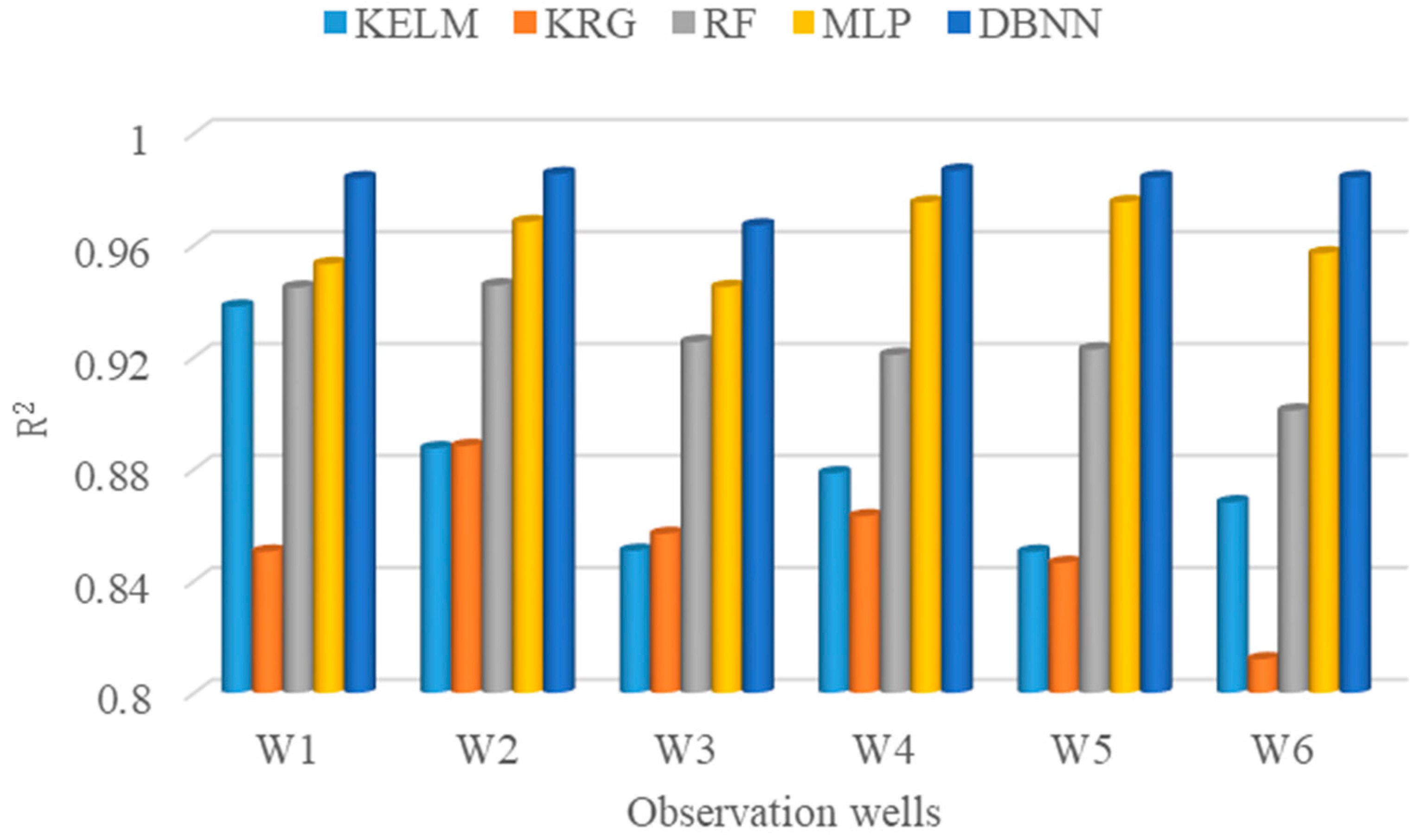
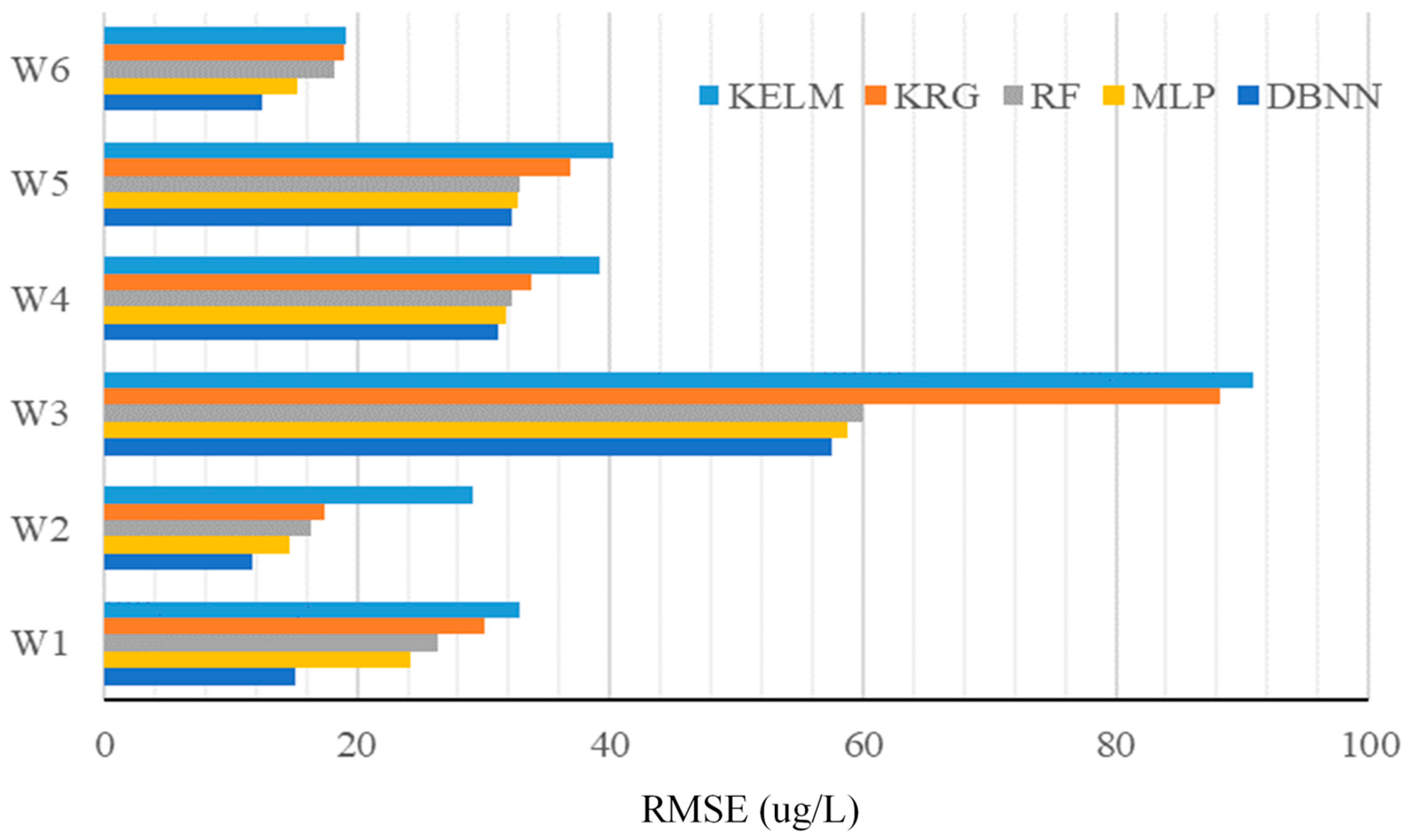
Construction of individual surrogate model. Individual surrogate models for each of the output locations, W1~W6, were developed using the KRG, KELM, MLP, RF, and DBN algorithms, as detailed in Section 3.2. Among them, the correlation function of KRG and the kernel function of KELM were chosen as Gaussian functions. MLP had five hidden layers, and the number of neurons was 128, 256, 256,128, and 128, respectively. RF consisted of 150 decision trees, DBN had three RBMs, and the number of neurons was 300, 350, and 200, respectively.

(3)

Establishment of Stacking ensemble surrogate model. From the five individual surrogate models, the MLP, RF, and DBN models, which exhibited higher accuracy, were selected as BLMs. Meta-data were generated from the BLMs’ outputs. Subsequently, a three-layer MLP model with 128 neurons in each layer served as the MLM to complete the construction of the Stacking ensemble surrogate model.

The accuracy of the trained models was evaluated using the testing dataset. Two performance metrics, the coefficient of determination (R²) and root mean squared error (RMSE), were employed to assess the accuracy of the surrogate models. The formulas were calculated as shown below, respectively:

$${\mathrm{R}}^2=1-{\displaystyle \frac{{\displaystyle \sum _{i=1}^n{\left(y_i-{\widehat{y}}_i\right)}^2}}{{\displaystyle \sum _{i=1}^n{\left(y_i-{\overline{y}}_i\right)}^2}}}$$

(16)

$$\mathrm{RMSE}=\sqrt{{\displaystyle \frac{1}{n}}{\displaystyle \sum _{i=1}^n{\left(y_i-{\widehat{y}}_i\right)}^2}}$$

(17)

where $n$ represents the number of test samples, $y_i$ denotes the output from the multiphase flow numerical simulation model, and ${\widehat{y}}_i$ represents the output from the surrogate model. A higher value of R², approaching 1, and lower values of RMSE indicate a more accurate surrogate model.

3.4. Application of the DE-MC Method

This study employed the DE-MC method for the GLCSI. The initial population size was set to 40, resulting in 40 parallel Markov chains exploring the solution space during the inversion process. The maximum number of iterations was set to 5000. Each individual in the population represented a potential solution for the set of identification variables. After the Markov chains converged, statistical analysis was performed on the converged samples to obtain point estimates and interval estimates for the variables, completing the inversion process. To reduce the computational time required for evaluating the likelihood function, which was necessary for accepting or rejecting proposed chains during algorithm iterations, the constructed Stacking ensemble surrogate model was utilized as a substitute for the simulation model.

4. Results

4.1. Performance of the Stacking Ensemble Surrogate Model

The performance of the individual surrogate models developed at locations W1~W6 using various methods was assessed based on Equations (16) and (17). The specific calculated results are presented in

Table 3. Accuracy index for five individual surrogate models at W1–W6.

Wells	Index	KELM	KRG	RF	MLP	DBNN
W1	R2	0.9380	0.8504	0.9448	0.9532	0.9839
	RMSE (μg/L)	32.82	30.06	26.41	24.27	15.19
W2	R2	0.8874	0.8882	0.9456	0.9682	0.9854
	RMSE (μg/L)	29.20	17.43	16.36	14.73	11.69
W3	R2	0.8508	0.8568	0.9254	0.9450	0.9670
	RMSE (μg/L)	177.86	88.21	60.05	58.84	57.60
W4	R2	0.8785	0.8631	0.9208	0.9752	0.9866
	RMSE (μg/L)	39.20	33.80	32.30	31.83	31.14
W5	R2	0.8504	0.8464	0.9227	0.9753	0.9841
	RMSE (μg/L)	40.25	36.86	32.84	32.64	32.21
W6	R2	0.8681	0.8120	0.9009	0.9570	0.9841
	RMSE (μg/L)	19.18	18.92	18.27	15.31	12.48

.

As indicated in Table 3, the DBN surrogate model consistently demonstrated the highest R² values and lowest RMSE values across all six observation wells among the five individual surrogate models. The R² values generally reached 0.98, with the exception of W3 where it achieved 0.96. To provide a clearer visual comparison of the relative performance of the individual surrogate models, bar charts comparing the R² and RMSE values for each model at different observation wells were presented in Figure 9 and Figure 10. These figures demonstrated that the RF, MLP, and DBN surrogate models, based on deep learning methods, exhibit superior performance with higher R² values and lower RMSE values compared to the KRG and KELM surrogate models, which were based on shallow learning methods. In accordance with the principle of selecting the best performers, the RF, MLP, and DBN models were chosen as BLMs for constructing the Stacking ensemble surrogate model, following the steps outlined in Section 3.3.

Table 4. Accuracy index for BLMs and ensemble model at W1–W6.

Wells	Index	BLM			Ensemble Model
		RF	MLP	DBNN	Stacking
W1	R2	0.9448	0.9532	0.9839	0.9975
	RMSE (μg/L)	26.41	24.27	15.19	10.48
W2	R2	0.9456	0.9682	0.9854	0.9950
	RMSE (μg/L)	16.36	14.73	11.69	8.72
W3	R2	0.9254	0.945	0.967	0.9896
	RMSE (μg/L)	60.05	58.84	57.60	35.66
W4	R2	0.9208	0.9752	0.9866	0.9969
	RMSE (μg/L)	32.30	31.83	31.14	28.41
W5	R2	0.9227	0.9753	0.9841	0.9943
	RMSE (μg/L)	32.84	32.64	32.21	30.58
W6	R2	0.9009	0.957	0.9841	0.9972
	RMSE (μg/L)	18.27	15.31	12.48	10.22

presents the accuracy indexes for the three BLMs and the Stacking ensemble surrogate model. The results indicate that the Stacking ensemble surrogate model demonstrates improved R² values and lower RMSE values compared to the BLMs. Figure 11 further illustrates this improvement by comparing the R² and RMSE values of the DBN model, which exhibits the best fitting performance among the BLMs, and the Stacking ensemble surrogate model at different observation wells. This figure visually confirmed that the Stacking ensemble surrogate model exhibits higher R² and lower RMSE. Figure 12 (W1–W6) demonstrates the comparison of the fitting effect between the output results of the three BLMs and the Stacking ensemble surrogate model on the testing sets and the output results of the simulation model. Figure 12 clearly shows that the scatter distribution of the Stacking ensemble surrogate model was more concentrated on the 1:1 trend line, and the fitting accuracy was higher. The results of the above figures and tables demonstrate that the Stacking ensemble surrogate model provided a more accurate approximation of the complex non-linear mapping relationship of the simulated model compared to the individual surrogate model. This enhanced accuracy made the Stacking ensemble model an effective alternative to the multiphase flow numerical simulation model, significantly improving the efficiency of subsequent GLCSI research.

This paper was based on the following computer hardware conditions: CPU: Intel Core i5-6500 3.20 GHz, 8 GB. In this study, the multiphase flow numerical simulation model took approximately 1200 s to run once. The DE-MC inversion process required approximately 200,000 calls to the simulation model, resulting in an estimated computation time of 2777.77 days. In contrast, the developed Stacking ensemble surrogate model took approximately 0.5 s to run once, leading to an estimated computation time of 1.15 days for the DE-MC inversion process. Adding the time required for training the surrogate model, which involves 800 calls to the simulation model (11.11 days), the total computation time for the Stacking ensemble surrogate model-based inversion process was approximately 12.25 days. This represents a 99.56% reduction in computational burden compared to the simulation model-based inversion process, with the total time for the ensemble surrogate model-based approach being only 0.44% of that for the simulation model-based approach.

4.2. DE-MC Inversion Results

The DE-MC method was employed to identify 19 unknown variables in the hypothetical case study. Figure 13 illustrates the variation in the convergence factor, calculated based on Equation (13), with respect to the iteration number. The figure indicated that the convergence factors satisfied the judgment criteria when the search iteration reached approximately 1500. The first 2000 iterations of the sample sequence were considered the “burning” phase, and the samples collected after 2000 iterations were deemed to follow the posterior distribution of the identification variables. This resulted in 3000 posterior samples for each identification variable. To mitigate the autocorrelation between these samples, a thinning operation was performed on the posterior samples, where a sample was periodically returned during the stable convergence phase [50]. In this study, every other sample was returned, resulting in 1500 posterior samples for each variable, which were subsequently used for statistical analysis.

This study applied principles of probability theory and mathematical statistics to conduct a statistical analysis of posterior samples for each unknown variable. This analysis enabled the derivation of point estimates, interval estimates, and estimations of the posterior probability distribution. The maximum posterior probability (MAP) value was selected as the point estimate for each unknown variable.

The eight variables were first analyzed as follows: porosity $n$, longitudinal and transverse aqueous-phase dispersion $\left({\alpha }_{wL},{\alpha }_{wT}\right)$, transverse and longitudinal coordinates of the pollution source $\left(L_x,L_y\right)$, initial and termination moments of the pollution release $\left(t_{on},t_{off}\right)$, and the release intensity $Q$ of the contamination source. The frequency distribution histograms and posterior probability density function curves (Figure 14a–h) were constructed to visualize the distributions of these variables. The left y-axis of each plot represents the frequency of samples, while the right y-axis denotes the posterior probability density. The red curve represents the posterior probability density curve, the orange dashed line with cross arrows indicates the true values of the unknown variables set manually in the hypothetical case, and the orange solid line with circular arrows represents the MAP values obtained through the DE-MC inversion.

Figure 14a–h clearly show that the posterior probability density distributions of the eight unknown variables obtained through the DE-MC inversion method exhibited distinct peaks. Furthermore, the MAP values were close to the true values set manually in the hypothetical case. Notably, although a second peak exists in the posterior probability density distribution of the variable $t_{off}$ (Figure 14g), the majority of the posterior samples were concentrated around the first peak, and the true value of the variable was closer to the first peak. This suggests that while local optima may exist, the adopted inversion method enabled sampling across the entire prior space, effectively escaping local optima and ultimately converging towards the true value.

Table 5. Point and interval estimation results for the unknown variables.

Variable	True Value	MAP Value	Relative Error	MRE	Posterior Distribution	Confidence Interval
						P0.025	P0.975
n	0.27	0.276	2.22%	2.79%	N(0.286, 0.0232)	0.25	0.332
αwL (m)	43.4	43.15	0.58%		N(45.61, 2.442)	40.73	50.49
αwT (m)	11.4	10.91	4.30%		N(11.37, 1.472)	9	14.31
Lx (m)	372	369.85	0.58%		N(335.76, 42.702)	250.36	390
Ly (m)	241	235.79	2.16%		N(237.50, 21.122)	200	279.74
ton (d)	599.55	623.57	4.01%		N(554.68, 102.422)	349.84	759.52
toff (d)	3980.44	3844.66	3.41%		N(3862.47, 109.522)	3643.47	4050
Q (m3/d)	2.96	2.81	5.07%		N(3.05, 1.632)	1	6.31

presents the point estimates (MAP values) of the inverted results obtained using the DE-MC method. The relative errors of the variables, calculated against their corresponding true values, were analyzed. The majority of the variables exhibited relative errors below 5%. The smallest relative errors were observed for ${\alpha }_{wL}$ and $L_x$, at 0.58%, while the largest error was observed for $Q$, at 5.07%. These findings demonstrate the effectiveness of the DE-MC method in achieving accurate estimations of the variables, with a mean relative error (MRE) of 2.79% across all variables.

The inversion process involved identifying 11 parameters controlling the log-permeability field, denoted as ${\xi }_1,{\xi }_2,\cdots ,{\xi }_{11}$. These parameters were assumed to follow a normal distribution for both the prior and posterior distributions. Therefore, probabilistic distribution estimations were not performed.

Table 6. Point estimates for 11 variables controlling for log-permeability fields.

Variable	True Value	MAP	Relative Error	MRE
ζ1	−0.13236	−0.12384	6.44%	4.54%
ζ2	−0.37932	−0.39072	3.01%
ζ3	0.05058	0.047864	5.37%
ζ4	0.13431	0.127399	5.15%
ζ5	−1.54757	−1.65037	6.64%
ζ6	−0.25961	−0.2593	0.12%
ζ7	0.38938	0.36831	5.41%
ζ8	0.86368	0.846544	1.98%
ζ9	0.19121	0.192888	0.88%
ζ10	−0.29933	−0.32131	7.34%
ζ11	−1.54274	−1.65988	7.59%

presents the point estimates for these 11 parameters, along with their calculated relative errors and the MRE.

The relative errors between the point estimates and the true values of the 11 variables shown in Table 6 were less than 10%, with the largest being 7.59%, the smallest 0.12%, and the MRE being only 4.54%. The 11 random numbers were then converted back to the form of the log-permeability field based on the point estimates in Table 6. Figure 15 shows the reference log-permeability field, the identified log-permeability field, and their calculated residual field. It was visually apparent that the inverted log-permeability field aligned well with the reference field, and the residuals were mainly distributed around zero. This suggests that the identification of the log-permeability field was highly accurate.

In conclusion, this study successfully completed the identification of 19 unknown variables in a hypothetical case study and evaluated the accuracy of the inversion process.

5. Conclusions and Discussion

This study presented a hypothetical LNAPL contamination site case and adopted the Stacking ensemble framework with QMC sampling to establish the ensemble surrogate for the simulation model, where source characteristics and model parameters were successfully inverted and identified. The conclusions of this study are as follows:

(1)

The QMC method can be employed to sample from the prior space of unknown variables, resulting in a more uniformly distributed and representative sample. This approach significantly enhanced the quality of the training data, leading to a more accurate and reliable surrogate model.

(2)

Compared to individual surrogate models, the Stacking ensemble surrogate model demonstrated a further enhancement in approximating the simulation model with an average R² value of 0.9950. Moreover, compared to the inversion process based on the simulation model, the computational burden was reduced by 99.56%

(3)

The DE-MC inversion algorithm demonstrated effectiveness in solving the 19-dimensional inversion problem. The average relative error for the eight unknown variables, excluding permeability, was 2.79%. For the 11 unknown variables characterizing the log-permeability field, the average relative error was 4.54%.

However, it is necessary to acknowledge that the limitation of this work is the failure to consider the impact of errors introduced by the application of the surrogate model on the inversion results. Some researchers have adopted certain methods to reduce these errors, such as Laloy et al. [51] implementing a two-stage MCMC simulation (i.e., fully exploring the parameter space using surrogate models in the first stage, and then evaluating the simulation model for correction in the second stage). In this study, this aspect was not explored in depth, and the method adopted calculated this part of the error directly into the observation error in the likelihood function. In our future work, we intend to analyze and quantify the impact of this type of error on the uncertainty of the inversion results.

References

- Huntley, D.; Beckett, G. Persistence of LNAPL sources: Relationship between risk reduction and LNAPL recovery. J. Contam. Hydrol. 2002, 59, 3–26. [Google Scholar] [CrossRef] [PubMed]
- Johnston, C.D.; Trefry, M.G. Characteristics of light nonaqueous phase liquid recovery in the presence of fine-scale soil layering. Water Resour. Res. 2009, 45, 5412. [Google Scholar] [CrossRef]
- Li, J.; Pang, Z.; Liu, Y.; Hu, S.; Jiang, W.; Tian, L.; Yang, G.; Jiang, Y.; Jiao, X.; Tian, J. Changes in groundwater dynamics and geochemical evolution induced by drainage reorganization: Evidence from 81Kr and 36Cl dating of geothermal water in the Weihe Basin of China. Earth Planet. Sci. Lett. 2023, 623, 118425. [Google Scholar] [CrossRef]
- Tomlinson, D.W.; Rivett, M.O.; Wealthall, G.P.; Sweeney, R.E. Understanding complex LNAPL sites: Illustrated handbook of LNAPL transport and fate in the subsurface. J. Environ. Manag. 2017, 204, 748–756. [Google Scholar] [CrossRef] [PubMed]
- Moghaddam, M.B.; Mazaheri, M.; Samani, J.M.V. Inverse modeling of contaminant transport for pollution source identification in surface and groundwaters: A review. Groundw. Sustain. Dev. 2021, 15, 100651. [Google Scholar] [CrossRef]
- Li, J.; Lu, W.; Fan, Y. Groundwater Pollution Sources Identification Based on Hybrid Homotopy-Genetic Algorithm and Simulation Optimization. Environ. Eng. Sci. 2021, 38, 777–788. [Google Scholar] [CrossRef]
- Singh, R.M.; Datta, B. Identification of Groundwater Pollution Sources Using GA-based Linked Simulation Optimization Model. J. Hydrol. Eng. 2006, 11, 1216–1227. [Google Scholar] [CrossRef]
- Chang, Z.; Lu, W.; Wang, H.; Li, J.; Luo, J. Simultaneous identification of groundwater contaminant sources and simulation of model parameters based on an improved single-component adaptive Metropolis algorithm. Hydrogeol. J. 2021, 29, 859–873. [Google Scholar] [CrossRef]
- Zanini, A.; Woodbury, A.D. Contaminant source reconstruction by empirical Bayes and Akaike’s Bayesian Information Criterion. J. Contam. Hydrol. 2016, 185–186, 74–86. [Google Scholar] [CrossRef]
- Wang, Z.; Lu, W.; Chang, Z.; Wang, H. Simultaneous identification of groundwater contaminant source and simulation model parameters based on an ensemble Kalman filter—Adaptive step length ant colony optimization algorithm. J. Hydrol. 2022, 605, 127352. [Google Scholar] [CrossRef]
- Zhang, J.; Zheng, Q.; Wu, L.; Zeng, L. Using Deep Learning to Improve Ensemble Smoother: Applications to Subsurface Characterization. Water Resour. Res. 2020, 56, e2020WR027399. [Google Scholar] [CrossRef]
- Forrester, A.I.; Keane, A.J. Recent advances in surrogate-based optimization. Prog. Aerosp. Sci. 2009, 45, 50–79. [Google Scholar] [CrossRef]
- Queipo, N.V.; Haftka, R.T.; Shyy, W.; Goel, T.; Vaidyanathan, R.; Tucker, P.K. Surrogate-based analysis and optimization. Prog. Aerosp. Sci. 2005, 41, 1–28. [Google Scholar] [CrossRef]
- Asher, M.J.; Croke, B.F.W.; Jakeman, A.J.; Peeters, L.J.M. A review of surrogate models and their application to groundwater modeling. Water Resour. Res. 2015, 51, 5957–5973. [Google Scholar] [CrossRef]
- Degen, D.; Voullième, D.C.; Buiter, S.; Franssen, H.-J.H.; Vereecken, H.; González-Nicolás, A.; Wellmann, F. Perspectives of physics-based machine learning strategies for geoscientific applications governed by partial differential equations. Geosci. Model Dev. 2023, 16, 7375–7409. [Google Scholar] [CrossRef]
- Mignot, E.; Dewals, B. Hydraulic modelling of inland urban flooding: Recent advances. J. Hydrol. 2022, 609, 127763. [Google Scholar] [CrossRef]
- Zhao, Y.; Qu, R.; Xing, Z.; Lu, W. Identifying groundwater contaminant sources based on a KELM surrogate model together with four heuristic optimization algorithms. Adv. Water Resour. 2020, 138, 103540. [Google Scholar] [CrossRef]
- Yongkai, A.; Wenxi, L.; Weiguo, C. Surrogate Model Application to the Identification of Optimal Groundwater Exploitation Scheme Based on Regression Kriging Method—A Case Study of Western Jilin Province. Int. J. Environ. Res. Public Health 2015, 12, 8897–8918. [Google Scholar] [CrossRef] [PubMed]
- Pan, F.; Zhu, P.; Zhang, Y. Metamodel-based lightweight design of B-pillar with TWB structure via support vector regression. Comput. Struct. 2010, 88, 36–44. [Google Scholar] [CrossRef]
- Wang, Z.; Lu, W.; Chang, Z.; Luo, J. A combined search method based on a deep learning combined surrogate model for groundwater DNAPL contamination source identification. J. Hydrol. 2023, 616, 128854. [Google Scholar] [CrossRef]
- Laloy, E.; Hérault, R.; Jacques, D.; Linde, N. Training-Image Based Geostatistical Inversion Using a Spatial Generative Adversarial Neural Network. Water Resour. Res. 2018, 54, 381–406. [Google Scholar] [CrossRef]
- Jeong, J.; Park, E. Comparative applications of data-driven models representing water table fluctuations. J. Hydrol. 2019, 572, 261–273. [Google Scholar] [CrossRef]
- Sun, W.; Trevor, B. A stacking ensemble learning framework for annual river ice breakup dates. J. Hydrol. 2018, 561, 636–650. [Google Scholar] [CrossRef]
- Heddam, S.; Ptak, M.; Zhu, S. Modelling of daily lake surface water temperature from air temperature: Extremely randomized trees (ERT) versus Air2Water, MARS, M5Tree, RF and MLPNN. J. Hydrol. 2020, 588, 125130. [Google Scholar] [CrossRef]
- Wu, Y.; Ke, Y.; Chen, Z.; Liang, S.; Zhao, H.; Hong, H. Application of alternating decision tree with AdaBoost and bagging ensembles for landslide susceptibility mapping. Catena 2020, 187, 104396. [Google Scholar] [CrossRef]
- Arsenault, R.; Gatien, P.; Renaud, B.; Brissette, F.; Martel, J.-L. A comparative analysis of 9 multi-model averaging approaches in hydrological continuous streamflow simulation. J. Hydrol. 2015, 529, 754–767. [Google Scholar] [CrossRef]
- Ouyang, Q.; Lu, W.; Lin, J.; Deng, W.; Cheng, W. Conservative strategy-based ensemble surrogate model for optimal groundwater remediation design at DNAPLs-contaminated sites. J. Contam. Hydrol. 2017, 203, 1–8. [Google Scholar] [CrossRef] [PubMed]
- Xing, Z.; Qu, R.; Zhao, Y.; Fu, Q.; Ji, Y.; Lu, W. Identifying the release history of a groundwater contaminant source based on an ensemble surrogate model. J. Hydrol. 2019, 572, 501–516. [Google Scholar] [CrossRef]
- Yin, J.; Tsai, F.T.-C. Bayesian set pair analysis and machine learning based ensemble surrogates for optimal multi-aquifer system remediation design. J. Hydrol. 2020, 580, 124280. [Google Scholar] [CrossRef]
- Xie, Y.; Sun, W.; Ren, M.; Chen, S.; Huang, Z.; Pan, X. Stacking ensemble learning models for daily runoff prediction using 1D and 2D CNNs. Expert Syst. Appl. 2023, 217, 119469. [Google Scholar] [CrossRef]
- Zounemat-Kermani, M.; Batelaan, O.; Fadaee, M.; Hinkelmann, R. Ensemble machine learning paradigms in hydrology: A review. J. Hydrol. 2021, 598, 126266. [Google Scholar] [CrossRef]
- Jiang, X.; Ma, R.; Wang, Y.; Gu, W.; Lu, W.; Na, J. Two-stage surrogate model-assisted Bayesian framework for groundwater contaminant source identification. J. Hydrol. 2021, 594, 125955. [Google Scholar] [CrossRef]
- Mo, S.; Lu, D.; Shi, X.; Zhang, G.; Ye, M.; Wu, J.; Wu, J. A Taylor Expansion-Based Adaptive Design Strategy for Global Surrogate Modeling with Applications in Groundwater Modeling. Water Resour. Res. 2017, 53, 10802–10823. [Google Scholar] [CrossRef]
- Yu, J.; Ai, M.; Ye, Z. A review on design inspired subsampling for big data. Stat. Pap. 2024, 65, 467–510. [Google Scholar] [CrossRef]
- Flowers-Cano, R.S.; Ortiz-Gómez, R.; León-Jiménez, J.E.; Rivera, R.L.; Cruz, L.A.P. Comparison of Bootstrap Confidence Intervals Using Monte Carlo Simulations. Water 2018, 10, 166. [Google Scholar] [CrossRef]
- Davey, K.R. Latin Hypercube Sampling and Pattern Search in Magnetic Field Optimization Problems. IEEE Trans. Magn. 2008, 44, 974–977. [Google Scholar] [CrossRef]
- Delshad, M.; Pope, G.; Sepehrnoori, K. A compositional simulator for modeling surfactant enhanced aquifer remediation, 1 formulation. J. Contam. Hydrol. 1996, 23, 303–327. [Google Scholar] [CrossRef]
- He, L.; Valocchi, A.J.; Duarte, C. An adaptive global–local generalized FEM for multiscale advection–diffusion problems. Comput. Methods Appl. Mech. Eng. 2024, 418, 116548. [Google Scholar] [CrossRef]
- Bratley, P.; Fox, B.L.; Niederreiter, H. Programs to generate Niederreiter’s low-discrepancy sequences. ACM Trans. Math. Softw. 1994, 20, 494–495. [Google Scholar] [CrossRef]
- Vandewoestyne, B.; Cools, R. On the convergence of quasi-random sampling/importance resampling. Math. Comput. Simul. 2010, 81, 490–505. [Google Scholar] [CrossRef]
- Sobol, I. On the distribution of points in a cube and the approximate evaluation of integrals. USSR Comput. Math. Math. Phys. 1969, 7, 784–802. [Google Scholar] [CrossRef]
- Wolpert, D.H. Stacked Generalization. Neural Netw. 1992, 5, 241–259. [Google Scholar] [CrossRef]
- Li, J.; Lu, W.; Wang, H.; Bai, Y.; Fan, Y. Groundwater contamination sources identification based on kernel extreme learning machine and its effect due to wavelet denoising technique. Environ. Sci. Pollut. Res. 2020, 27, 34107–34120. [Google Scholar] [CrossRef]
- Oliver, M.A.; Webster, R. A tutorial guide to geostatistics: Computing and modelling variograms and kriging. Catena 2014, 113, 56–69. [Google Scholar] [CrossRef]
- Gholami, V.; Chau, K.; Fadaee, F.; Torkaman, J.; Ghaffari, A. Modeling of groundwater level fluctuations using dendrochronology in alluvial aquifers. J. Hydrol. 2015, 529, 1060–1069. [Google Scholar] [CrossRef]
- Breiman, L. Random forests. Mach. Learn. 2001, 45, 5–32. [Google Scholar] [CrossRef]
- Hinton, G.E.; Osindero, S.; Teh, Y.-W. A Fast Learning Algorithm for Deep Belief Nets. Neural Comput. 2006, 18, 1527–1554. [Google Scholar] [CrossRef]
- Braak, C.J.F.T.; Vrugt, J.A. Differential Evolution Markov Chain with snooker updater and fewer chains. Stat. Comput. 2008, 18, 435–446. [Google Scholar] [CrossRef]
- Brooks, S.P.; Roberts, G.O. Convergence assessment techniques for Markov chain Monte Carlo. Stat. Comput. 1998, 8, 319–335. [Google Scholar] [CrossRef]
- Bai, Y.; Lu, W.; Li, J.; Chang, Z.; Wang, H. Groundwater contamination source identification using improved differential evolution Markov chain algorithm. Environ. Sci. Pollut. Res. 2022, 29, 19679–19692. [Google Scholar] [CrossRef]
- Laloy, E.; Rogiers, B.; Vrugt, J.A.; Mallants, D.; Jacques, D. Efficient posterior exploration of a high-dimensional groundwater model from two-stage Markov chain Monte Carlo simulation and polynomial chaos expansion. Water Resour. Res. 2013, 49, 2664–2682. [Google Scholar] [CrossRef]