Modification and Improvement of the Churchill Equation for Friction Factor Calculation in Pipes

Abstract

Accurate prediction of the friction factor is fundamental for designing and calibrating fluid transport systems. While the Colebrook–White equation is the benchmark for precision due to its physical basis, its implicit nature hinders practical applications. Explicit correlations like Churchill’s equation are commonly used but often sacrifice accuracy. This study introduces two novel modifications to Churchill’s equation to enhance predictive capabilities. Developed through a rigorous analysis of 240 test cases and validated against a dataset of 21,000 experiments, the proposed Churchill B(Re) and Churchill B(V,ε) models demonstrate significantly improved accuracy compared to the original Churchill equation. The development of these functions was achieved through generalized reduced gradient (GRG) nonlinear optimization. This optimized equation offers a practical and precise alternative to the Colebrook–White equation. The mean relative errors (MRE) for the modified models, Churchill B(Re) and Churchill B(V,ε), are 0.025% and 0.807%, respectively, indicating a significant improvement over the original equation introduced by Churchill in 1973, which exhibits an MRE of 0.580%. Similarly, the mean absolute errors (MAE) are 0.0008% and 0.0154%, respectively, compared to 0.0291% for the original equation. Beyond practical applications, this research contributes to a deeper understanding of friction factor phenomena and establishes a framework for refining other empirical correlations in the field.

1. Introduction

In fluid transport systems engineering, a fundamental aspect lies in understanding and quantifying the frictional interaction between moving fluids and the internal surface of conduits. The flow of a fluid through a pipe causes energy losses due to friction between fluid molecules and pipe walls [1]. This phenomenon is characterized by a parameter that quantifies the inherent resistance to flow [2], has a considerable impact on the performance, and operational efficiency of such systems [3]. Fluid transport through closed conduits, such as pipes, is a fundamental aspect of fluid dynamics. It has a rich history of research and development, and a wide range of practical applications in various fields such as energy, transportation, and industry [4]. Explicit correlations are essential in fluid dynamics, offering several advantages, including ease of implementation, faster computations, and enhanced insight into fluid behavior. These explicit correlations are particularly valuable in educational settings and for broader accessibility because they strike a balance between reasonable accuracy and practicality in engineering applications.

Central to this field is the dimensionless friction factor (f), used to calculate pressure drops due to frictional losses in internal pipe flows. This factor is dependent on two key parameters: the Reynolds number (Re) and the relative surface roughness (ε/D). The Reynolds number is a dimensionless quantity that is calculated based on the other input parameters, as it is a derived quantity that depends on the velocity, diameter, and coefficient of kinematic fluid viscosity. It is used to characterize the flow regime of a fluid and is an important input for calculating the friction factor.

For laminar flow (Re < 2320), the friction factor, f, can be calculated using the Hagen–Poiseuille equation [5], as shown in Equations (1) and (2), which are the equations for Darcy–Weisbach and Fanning, respectively.

$${\mathrm{f}}_{\mathrm{D}}={\displaystyle \frac{64}{\mathrm{R}\mathrm{e}}}$$

(1)

$${\mathrm{f}}_{\mathrm{F}}={\displaystyle \frac{16}{\mathrm{R}\mathrm{e}}}$$

(2)

where f_D is the friction factor used in the Darcy–Weisbach head-loss equation (Equation (3)) and f_F is the friction factor used in the head-loss equation expressed by Fanning (Equation (4)). Head loss, denoted as hf_D and hf_F, represents the energy dissipated per unit weight of fluid due to friction as it flows through a pipe. It is typically expressed in units of length and can be calculated using the Darcy–Weisbach Equation (3).

$${\mathrm{h}}_{{\mathrm{f}}_{\mathrm{D}}}={\mathrm{f}}_{\mathrm{D}}\left({\displaystyle \frac{\mathrm{L}}{\mathrm{D}}}\right)\left({\displaystyle \frac{{\mathrm{V}}^2}{2\mathrm{g}}}\right)$$

(3)

$${\mathrm{h}}_{{\mathrm{f}}_{\mathrm{F}}}={2\mathrm{f}}_{\mathrm{F}}\left({\displaystyle \frac{\mathrm{L}}{\mathrm{D}}}\right)\left({\displaystyle \frac{{\mathrm{V}}^2}{\mathrm{g}}}\right)$$

(4)

where hf_D is the head loss due to friction, expressed in units of length (e.g., meters); f_D is the Darcy friction factor, a dimensionless constant that depends on the roughness of the pipe and the properties of the fluid; L is the length of the pipe, expressed in units of length (e.g., meters); D is the internal diameter of the pipe, expressed in units of length (e.g., meters); V is the average velocity of the fluid, expressed in units of length per unit time (e.g., meters per second); g is the acceleration due to gravity, approximately 9.81 m per second squared. Both friction factors are related by Equation (5).

$${\mathrm{f}}_{\mathrm{D}}={4\mathrm{f}}_{\mathrm{F}}$$

(5)

For turbulent flow (4000 < Re < 100,000) in smooth pipes, f can be approximated with Blasius Equations (6) and (7) [1].

$${\mathrm{f}}_{\mathrm{D}}={\displaystyle \frac{0.316}{{\mathrm{R}\mathrm{e}}^{0.25}}}$$

(6)

$${\mathrm{f}}_{\mathrm{F}}={\displaystyle \frac{0.079}{{\mathrm{R}\mathrm{e}}^{0.25}}}$$

(7)

For turbulent flow (Re > 4000) in rough pipes, the friction factor (f) depends on both the Reynolds number (Re) and the relative roughness (ε/D). The Colebrook–White equation [6] enables the implicit calculation of the friction factor, f, in terms of Re and ε/D.

The friction factor is commonly expressed using the Moody diagram [7], which provides a graphical representation of the Colebrook–White equation and allows for the visual determination of the friction factor, f, within ranges of the Reynolds number and relative roughness [8,9,10,11].

It is important to acknowledge the seminal contributions of Johann Nikuradse in the field of fluid dynamics, particularly his work on pipe flow and friction factors. In the 1930s, Nikuradse conducted extensive experiments on fluid flow in pipes with varying degrees of roughness. His research, published in 1933 [12], laid the groundwork for understanding the relationship between pipe roughness, Reynolds number, and friction factor. Nikuradse’s experiments and the resulting empirical expressions predated the work of Colebrook and White by nearly two decades and Churchill’s contributions by about four decades. His findings on the effects of relative roughness and the transition between smooth and fully rough pipe flow were instrumental in shaping our current understanding of fluid dynamics in pipes. The subsequent work by Colebrook and White, and later Churchill, can be seen as refinements and extensions of Nikuradse’s pioneering research, adapting his insights to a wider range of flow conditions and pipe characteristics [12].

Researchers have formulated various explicit approximations to the Colebrook–White equation, such as the equations of Wood [13], Churchill [14], Chen [15], Barr [16], Churchill and Chan [17], Haaland [18], Swamee and Jain [19], and many others [20]. These provide reasonably accurate estimates of (f) for specific ranges of Re and ε/D [21].

More recently, data-based techniques such as artificial neural networks [22], neuro-fuzzy systems, and model trees [23,24] have been used to predict the friction factor, f. These can provide highly accurate predictions over wide ranges of Re and ε/D.

The development of new explicit equations for the determination of f continues to be an area of focus, seeking simplicity and precision over wide ranges of parameters [25] and capturing subtle behaviors such as transition roughness [26]. Validation of these equations against experimental data remains crucial in this field of study [27]. The development of accurate correlations for fluid flow behavior is fundamental for predicting the friction factor with high precision. This study aims to provide a more precise mathematical representation of the Churchill [14,28] 1973 friction factor equation, which is widely used in the prediction of friction factors in pipe flows. The goal is to approximate the Colebrook–White [6] equation as closely as possible.

Two new mathematical expressions are proposed: Churchill B(V,ε) and Churchill B(Re), both based on a subtraction term B that depends on dimensional parameters. For Churchill B(V,ε), B depends on velocity and roughness, while for Churchill B(Re), B depends on dimensionless parameters, such as Reynolds number and relative roughness.

These expressions were developed based on an analysis of 240 primary cases and validated using 21,000 experimental data points. The precision of each expression was evaluated using the percentage of absolute errors and the percentage of relative errors compared to the Colebrook–White [6] equation. The results show that the expression based on dimensionless parameters, Churchill B(Re), provides the most accurate results, with the lowest percentage of errors. The proposed expression was demonstrated to improve the precision of the friction factor calculation in pipelines transporting pressurized fluids, and it was compared to its original form, as presented by Churchill 1973 [28] and Churchill 1977 [14].

2. Materials and Methods

The friction factor f can be determined using the implicit Colebrook–White [6] equation for Darcy–Weisbach, as shown in Equation (8). This expression describes the friction factor based on the relative roughness of the pipe and the Reynolds number.

$${\displaystyle \frac{1}{\sqrt{{\mathrm{f}}_{\mathrm{D}}}}}=-2{\mathrm{l}\mathrm{o}\mathrm{g}}_{10}\left[{\displaystyle \frac{\mathrm{ℇ}}{\left(3.71\mathrm{D}\right)}}+{\displaystyle \frac{2.51}{\left(\mathrm{R}\mathrm{e}\sqrt{{\mathrm{f}}_{\mathrm{D}}}\right)}}\right]$$

(8)

According to Wilkes [5], the expression presented as Equation (9), which corresponds to the Colebrook–White [6] equation, is considered a good representation of the friction factor used in the Fanning head-loss equation, experimentally determined in the turbulent region.

$$\left\{\begin{array}{c}{\displaystyle \frac{1}{\sqrt{{\mathrm{f}}_{\mathrm{F}}}}}=2.28-4 {\mathrm{l}\mathrm{o}\mathrm{g}}_{10}\left[{\displaystyle \frac{\mathrm{ℇ}}{\mathrm{D}}}+{\displaystyle \frac{4.67}{\mathrm{R}\mathrm{e}\sqrt{{\mathrm{f}}_{\mathrm{F}}}}}\right]\\ \\ {\displaystyle \frac{1}{\sqrt{{\mathrm{f}}_{\mathrm{F}}}}}=-1.7370 \mathrm{l}\mathrm{n}\left[0.269\left({\displaystyle \frac{\mathrm{ℇ}}{\mathrm{D}}}\right)+{\displaystyle \frac{1.2570}{\mathrm{R}\mathrm{e}\sqrt{{\mathrm{f}}_{\mathrm{F}}}}}\right]\end{array}\right\}$$

(9)

The Colebrook–White equation is an implicit mathematical expression, which requires the use of numerical iterative (recursive) methods for its solution, such as the fixed-point method or the Newton–Raphson method, which are widely used in this context [29,30].

In this study, the Newton–Raphson method was applied to solve Equation (8), similar to what was reported by Zigrang and Sylvester [31], and an algorithm flowchart was developed for its implementation, as presented in Figure 1.

The algorithm in Figure 1 requires the following input parameters: Reynolds number (Re), absolute roughness (ε), and internal diameter of the pipe (D). The mathematical process converges to the desired result after several iterations, satisfying the equations and boundary constraints [16,32], and finally obtaining the calculated friction factor, f, with a precision of convergence of 1 × 10⁻¹².

In 1973, Churchill [28] proposed Equation (10) as an explicit alternative for estimating the friction factor, f. According to Churchill [28], this expression matches the derivative of the Colebrook–White [6] equation through heuristic reasoning when the head loss is specified. Its technically used version is presented through Equation (11).

$${\mathrm{e}}^{-{\displaystyle \frac{\mathrm{V}}{2.46}} \sqrt{{\displaystyle \raisebox{1ex}{$\mathsf{\tau }$}\!\left/ \!\raisebox{-1ex}{$\mathsf{\rho }$}\right.}}}={\displaystyle \frac{\mathrm{ℇ}}{\left(3.7\mathrm{D}\right)}}+{\left({\displaystyle \frac{7\mathsf{\nu }}{\mathrm{D}\mathrm{V}}}\right)}^{0.9}$$

(10)

$${\displaystyle \frac{1}{\sqrt{\mathrm{f}}}}=-2{\mathrm{l}\mathrm{o}\mathrm{g}}_{10}\left[{\displaystyle \frac{\mathrm{ℇ}}{\left(3.7\mathrm{D}\right)}}+{\left({\displaystyle \frac{7}{\mathrm{R}\mathrm{e}}}\right)}^{0.9}\right]$$

(11)

where ℇ is the absolute roughness of the internal walls of the pipe in m, D is the internal diameter in m, Re is the Reynolds number, f is the friction factor for the Darcy–Weisbach equation, V is the average flow velocity in m/s, τ is the shear stress at the tube wall in N/m², ρ is the fluid density in kg/m³, and ν is the kinematic viscosity coefficient in m²/s. Shear stress is responsible for energy losses due to friction. It is the force per unit area on the internal surface of the pipe or between different layers of the flow field, caused by the fluid’s viscosity. In one of its simplified forms, it can be expressed as the product of the fluid’s specific weight, the hydraulic radius, and the friction slope of the flow in the pipe. The interrelation between head loss and shear stress is that they are both related to the friction between the fluid and the pipe walls. The shear stress at the pipe walls is a measure of the force exerted by the fluid on the walls, while the head loss is a measure of the energy that is lost due to this friction [33]. The friction factor, f, is a dimensionless quantity that is used to quantify the friction between the fluid and the pipe walls. It is related to the Reynolds number, the relative roughness of the pipe, and the shear stress at the pipe walls.

Churchill [28] proposed a correlation for the friction factor that has been widely used and cited in specialized literature. This correlation, presented in Equation (11), is explicit and has been cited by notable authors such as Eck [34], Swamee and Jain [19], Churchill [14], Shacham [32], Barr [16], Serghides [35], Zigrang and Sylvester [31], Sonnad and Goudar [36], Avci and Karagoz [37], Papaevangelou [21], and Genić et al. [8], among others. Although the equation of Churchill [36] remains valid, in recent years, several alternative explicit correlations with higher precision and ease of use have been proposed compared to the original implicit Colebrook–White equation [38].

Churchill [14] proposed the original mathematical expression, extending his previous work to encompass the entire range of laminar and turbulent flow (Equations (12)–(14)). Later studies by Genić et al. [8] evaluated the accuracy of the Churchill correlation against other explicit equations, finding good performance within its recommended applicability range. Brkić [39] and Asker et al. [40] further support the Churchill equation as a valuable tool for estimating the friction factor in turbulent flows across all Reynolds number ranges.

$$\mathrm{f}=8{\left[{\left({\displaystyle \frac{8}{\mathrm{R}\mathrm{e}}}\right)}^{12}+{\displaystyle \frac{1}{{\left(\mathrm{A}+\mathrm{B}\right) }^{\frac{3}{2}}}} \right]}^{{\displaystyle \frac{1}{12}}}$$

(12)

$$\mathrm{A}={\left[2.457\mathrm{l}\mathrm{n}\left({\displaystyle \frac{1}{{\left(\frac{7}{\mathrm{R}\mathrm{e}}\right)}^{0.9}+0.27\left(\frac{\mathrm{ℇ}}{\mathrm{D}}\right)}}\right)\right]}^{16}$$

(13)

$$\mathrm{B}={\left( {\displaystyle \frac{37530}{\mathrm{R}\mathrm{e}}} \right)}^{16}$$

(14)

$$\forall \left\{\begin{array}{c}4\times {10}^3<Re<1\times {10}^8\\ \\ 1\times {10}^{-6}<\left({\displaystyle \frac{\mathrm{ℇ}}{\mathrm{D}}}\right)<0.05\end{array}\right\}$$

2.1. Proposed Mathematical Model Based on Dimensional Parameters, Velocity, and Roughness: The Churchill B(V,ε) Function

This study aimed to develop and validate a modification of the Churchill [28] equation for calculating the friction factor in pressure piping. This modification, called the Churchill B(V,ε) function and presented in Equation (15), along with the subtracting function in Equation (16), offers several significant advantages. First, it provides an explicit solution for the friction factor (f), which simplifies the calculation process compared to implicit equations, such as those studied by Brkić [30] and Genić et al. [8]. Additionally, the new function contains only one logarithm, making it more accessible compared to other explicit expressions used in fluid engineering [21]. Following a similar approach as Vatankhah [41] in a different context, this study developed an approximate explicit solution for the Colebrook–White equation. This solution, inspired by the work of Zigrang and Sylvester [31], aims to reduce computational resources by minimizing the dependence on logarithms and non-integer powers.

$$\mathrm{f}={\left\{-2\mathrm{L}\mathrm{o}\mathrm{g}\left[\left(\left({\displaystyle \frac{\mathrm{ℇ}}{3.7\mathrm{D}}}\right)+{\left({\displaystyle \frac{7-\mathrm{B}}{{\mathrm{R}\mathrm{e}}^{0.982}}}\right)}^{0.9}\right)\right]\right\}}^{-2}$$

(15)

where ε and D are expressed in meters.

$$\mathrm{B}=1.0413964+0.0443562\left(\mathrm{V}\right)+9.27075{\left(1000\mathsf{\epsilon }\right)}^{0.838875}$$

(16)

The B function, which is a subtracting term in Churchill’s [28] Equation (11), consists of three terms: a constant, a linear term proportional to the velocity (V, in m/s), and an exponential nonlinear term dependent on the absolute roughness (ε, in m), hereafter referred to as the Churchill B(V,ε) function.

Statistical Methodology

In this study, a rigorous statistical methodology was employed to validate the proposed modification to the Churchill [28] equation. The new Churchill B(V,ε) function was compared with the Churchill models of 1977 and 1973, Haaland, Barr, Swamee and Jain, and Pavlov correlations in 240 test cases.

The Colebrook–White equation is chosen as the benchmark for comparison due to its physically based formulation, which accurately accounts for the complex interactions between fluid flow and pipe roughness. Proposed by Colebrook and White in 1937 [6], this equation has been extensively validated through experimental and numerical studies [42] and is widely recognized as a fundamental reference for friction factor calculations. Therefore, the proposed functions, derived from the Churchill 1973 equation, are evaluated against the Colebrook–White equation to assess their accuracy and reliability in predicting friction factors.

To assess the accuracy of the newly proposed equations, Churchill B(V,ε) and Churchill B(Re), relative and absolute errors were calculated. These errors were determined by comparing the results with those obtained from the benchmark Colebrook–White equation. Furthermore, the standard error of the estimation (S) was employed as a key metric to evaluate the model’s precision.

A rigorous validation process involving 21,000 experiments confirmed the robustness and reliability of the modified Churchill equations. This comprehensive evaluation enabled a thorough assessment of the new equations’ effectiveness in reducing errors and improving accuracy compared to existing methods.

2.2. Proposed Mathematical Model Based on Dimensionless Parameters, Reynolds Number and Relative Roughness: The Churchill B(Re) Function

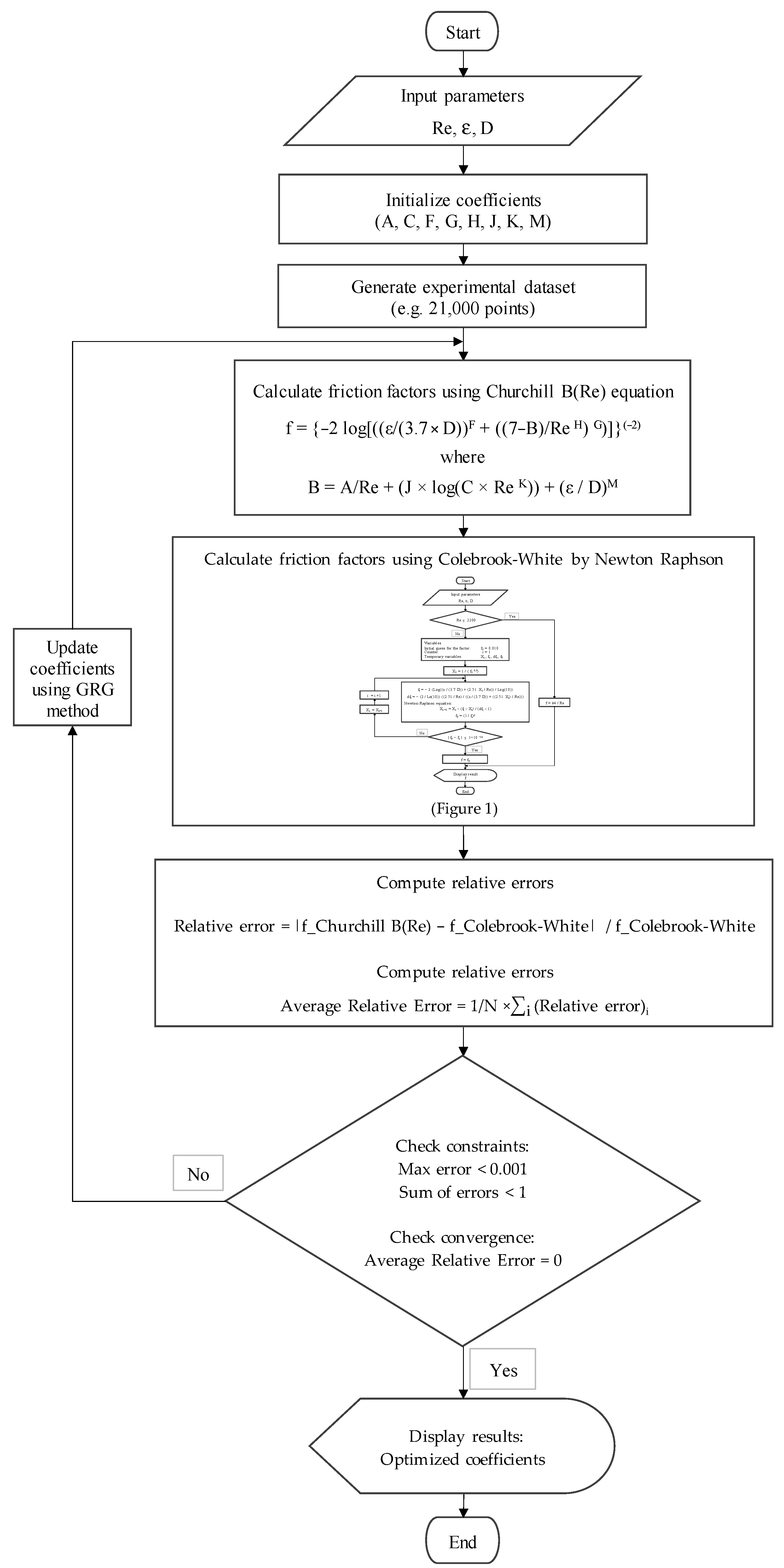
2.2.1. GRG Nonlinear Optimization

The Generalized Reduced Gradient (GRG) method is an iterative technique used for solving nonlinear optimization problems with constraints. It is particularly effective in finding the local minima of an objective function when both the objective function and the constraints are nonlinear [43]. Below is a detailed mathematical foundation of the GRG method.

• Formulation of the Optimization Problem

The formulation is based on the following nonlinear optimization problem:

$$\begin{gathered} \min \mathrm{f}\left(\mathrm{x}\right) \\ \mathrm{s}\mathrm{u}\mathrm{b}\mathrm{j}\mathrm{e}\mathrm{t} \mathrm{t}\mathrm{o}: \\ {\mathrm{g}}_{\mathrm{i}}\left(\mathrm{x}\right)=0,\mathrm{i}=1,2,\dots ,\mathrm{m} \\ {\mathrm{h}}_{\mathrm{j}}\left(\mathrm{x}\right)=0,\mathrm{i}=1,2,\dots ,\mathrm{m} \end{gathered}$$

where x ∈ ℝⁿ is the vector of decision variables.

The f(x): ℝⁿ → ℝ is the vector of decision variables,

The g_i(x): ℝⁿ → ℝ are the equality constraints,

The h_i(x): ℝⁿ → ℝ are the inequality constraints.

b.

Concept of Reduced Gradients

The GRG method was employed based on the concept of reduced gradients. The study considered the feasible region and the manner of movement within this region. It was assumed that a feasible point x_k was reached, and the nearby feasible subspace was defined by the active constraints at x_k. The active constraints were those inequality constraints h_j(x) ≤ 0 that were satisfied with equality at x_k.

c.

Feasible Direction

To move within the feasible region, a direction d is sought such that xk + d remains feasible. This implies that the movement must respect the active constraints. The feasible direction d is determined by solving the following linear system:

J_g(x_k) d = 0
J_h(x_k) d ≤ 0

where J_g(x_k) is the Jacobian matrix of the equality constraints and J_h(x_k) is the Jacobian matrix of the active inequality constraints at point x_k.

d.

Lagrangian Function

The GRG method employs the Lagrangian function to incorporate the constraints into the objective function. The Lagrangian function is defined as shown in Equation (17).

$$\mathrm{L}\left(\mathrm{x},\mathsf{\lambda },\mathsf{\mu }\right)=\mathrm{f}\left(\mathrm{x}\right)+\sum _{\mathrm{i}=1}^{\mathrm{m}}{\mathsf{\lambda }}_{\mathrm{i}}{\mathrm{g}}_{\mathrm{i}}\left(\mathrm{x}\right)+\sum _{\mathrm{j}=1}^{\mathrm{p}}{\mathsf{\mu }}_{\mathrm{j}}{\mathrm{h}}_{\mathrm{j}}\left(\mathrm{x}\right)$$

(17)

where L(x, λ, μ) denotes the Lagrangian function, which is a function that combines the objective function f(x) with the constraints ${\mathrm{g}}_{\mathrm{i}}\left(\mathrm{x}\right)$ and ${\mathrm{h}}_{\mathrm{j}}\left(\mathrm{x}\right)$. x is the vector of decision variables, which are the values that are being optimized. f(x) is the objective function, which is the function that is being optimized. ${\mathsf{\lambda }}_{\mathrm{i}}$ are the Lagrange multipliers associated with the equality constraints [44]. ${\mathsf{\mu }}_{\mathrm{j}}$ are the Lagrange multipliers associated with the inequality constraints. ${\mathrm{g}}_{\mathrm{i}}\left(\mathrm{x}\right)$ are the equality constraints, which are the constraints that must be satisfied with equality. ${\mathrm{h}}_{\mathrm{j}}\left(\mathrm{x}\right)$are the inequality constraints, which are the constraints that must be satisfied with inequality.

e.

Karush–Kuhn–Tucker (KKT) Conditions

For a point ${\mathrm{x}}^{*}$ to be optimal, it must satisfy the KKT conditions:

○

Stationarity Condition, Equation (18):

$$\nabla \mathrm{f}\left({\mathrm{x}}^{*}\right)+\sum _{\mathrm{i}=1}^{\mathrm{m}}{\mathsf{\lambda }}_{\mathrm{i}}\nabla {\mathrm{g}}_{\mathrm{i}}\left({\mathrm{x}}^{*}\right)+\sum _{\mathrm{j}=1}^{\mathrm{p}}{\mathsf{\mu }}_{\mathrm{j}}{\nabla \mathrm{h}}_{\mathrm{j}}\left({\mathrm{x}}^{*}\right)=0$$

(18)

where $\nabla \mathrm{f}\left({\mathrm{x}}^{*}\right)$ is the gradient of the objective function with respect to the decision variables, which is a vector of partial derivatives of the objective function evaluated at the optimal point ${\mathrm{x}}^{*}$ [45]. $\nabla {\mathrm{g}}_{\mathrm{i}}\left({\mathrm{x}}^{*}\right)$are the gradients of the equality constraints with respect to the decision variables, which are vectors of partial derivatives of the equality constraints evaluated at the optimal point ${\mathrm{x}}^{*}$. ${\nabla \mathrm{h}}_{\mathrm{j}}\left({\mathrm{x}}^{*}\right)$ are the gradients of the inequality constraints with respect to the decision variables, which are vectors of partial derivatives of the inequality constraints evaluated at the optimal point ${\mathrm{x}}^{*}$.

○

Primal Feasibility Condition:

$$\begin{gathered} {\mathrm{g}}_{\mathrm{i}}\left({\mathrm{x}}^{\mathrm{*}}\right)=0,\forall \mathrm{i} \\ {\mathrm{h}}_{\mathrm{j}}\left({\mathrm{x}}^{\mathrm{*}}\right)=0,\forall \mathrm{j} \end{gathered}$$

○

Dual Feasibility Condition:

$${\mathsf{\mu }}_{\mathrm{j}}>0,\forall \mathrm{j}$$

○

Complementarity Condition:

$${\mathsf{\mu }}_{\mathrm{j}}{\mathrm{h}}_{\mathrm{j}}\left({\mathrm{x}}^{\mathrm{*}}\right)=0,\forall \mathrm{j}$$

f.

GRG Method Algorithm

The GRG algorithm follows these iterative steps [46,47]:

• Initialization: Choose an initial feasible point x₀. Set initial values for the Lagrange multipliers.
• Search Direction: Compute the search direction d_k using the reduced gradient.
• Update: Update the current point: ${\mathrm{x}}_{\mathrm{k}+1}={\mathrm{x}}_{\mathrm{k}}+{\propto }_{\mathrm{k}}{\mathrm{d}}_{\mathrm{k}}$, where ${\propto }_{\mathrm{k}}$ is the step size determined by a line search procedure.
• Convergence Check: Check if the KKT conditions are satisfied within a predefined tolerance.
• Iteration: If not converged, update the Lagrange multipliers and repeat from Step 2.

g.

Implementation Details

Implementing the GRG method requires: Efficiently calculating gradients and Jacobians, solving linear systems to determine feasible directions, performing line searches to ensure sufficient improvement in the objective function, and properly handling active and inactive inequality constraints.

2.2.2. Optimization of Churchill B(Re)’s Friction Factor Equation Using Generalized Reduced Gradient Method

This study formulated an optimization problem to minimize the average relative error between the proposed Churchill’s B(Re) equation and the Colebrook–White equation across 21,000 experimental points, subject to constraints such as the maximum relative error below 10⁻³ and the sum of all relative errors less than 1. The Generalized Reduced Gradient (GRG) method was employed for its robustness in handling nonlinear optimization problems, using a precision of constraints of 10⁻⁷, integer optimality of 1%, GRG Nonlinear convergence of 10⁻⁶, and forward derivatives.

The optimization model GRG Nonlinear employed in this study is presented in Figure 2, which depicts the process of the model.

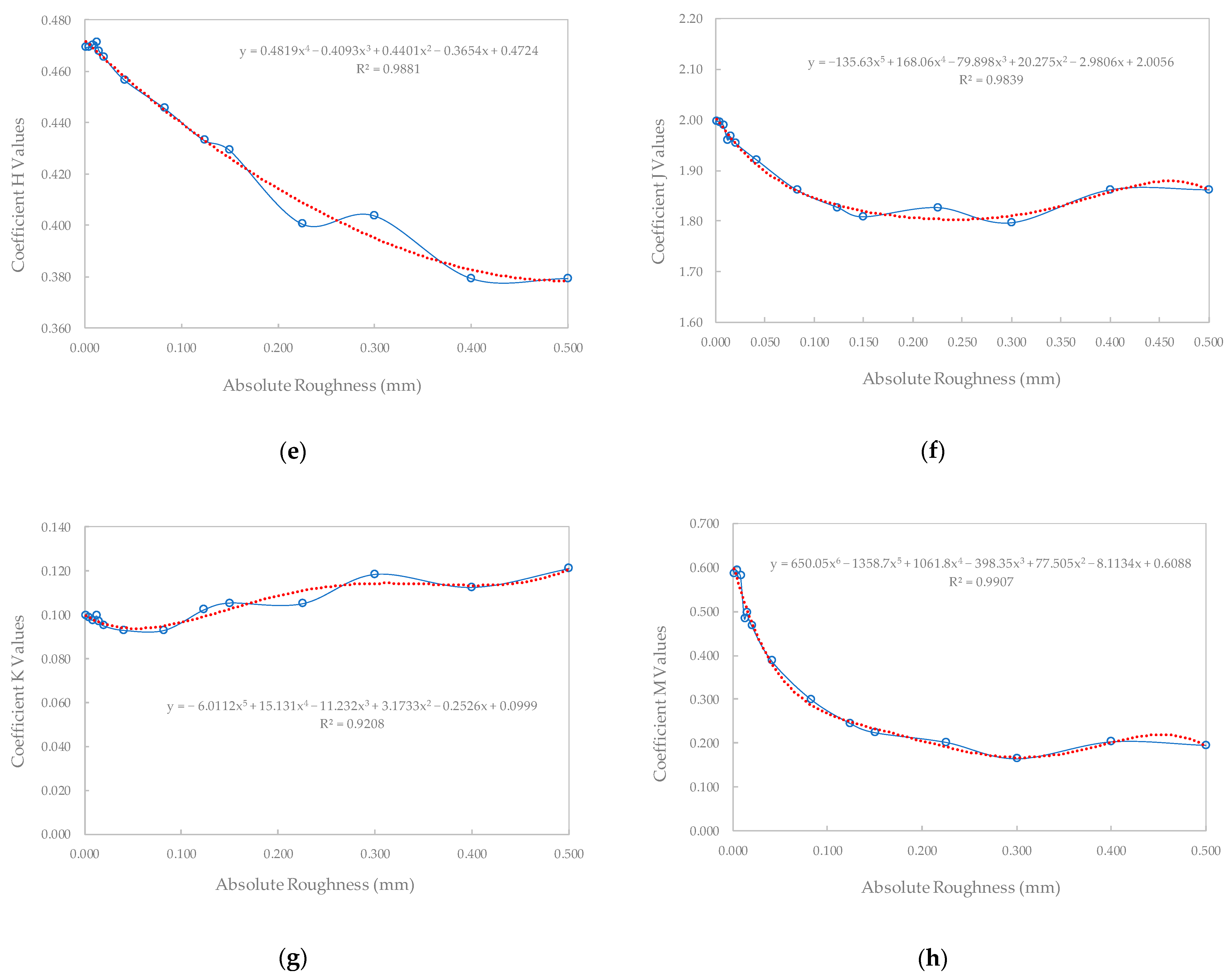
2.2.3. Proposed Function for the Churchill B(Re) Function

A second modification to the Churchill [28] equation for calculating the friction factor in pressurized pipes is presented. This modification is named the Churchill B(Re) function. This function and its corresponding subtraction expression (B(Re)) were obtained through the analysis of 21,000 experiments, which involved 1500 different Reynolds numbers for each of the 14 roughness values examined.

The proposed Churchill B(Re) function also provides an explicit solution for the friction factor (f), simplifying the calculation process compared to implicit equations. Additionally, the new functions contain only a single logarithm, making them more accessible compared to other explicit expressions used in fluid engineering.

The proposed functions address limitations observed in existing equations and provide a more precise and accessible solution for estimating the friction factor in pressurized pipes. It is important to note that the proposed Churchill B(V,ε) and Churchill B(Re) functions represent a novel approach that improves the precision in estimating the friction factor. This approach addresses limitations observed in existing equations, including those based on Equations (15), (16), (19) and (20), which are not based on the works of Vatankhah [41] or Zigrang and Sylvester [31]. Specifically, this approach provides a more accurate estimation of the friction factor across a wide range of Reynolds Numbers and Relative Roughness values.

The proposed Churchill B(Re) function is based on Equation (19), which is a modification of the original Churchill [28] equation.

$$\mathrm{f}={\left\{-2\mathrm{L}\mathrm{o}\mathrm{g}\left[\left({\left({\displaystyle \frac{\mathrm{ℇ}}{3.7\mathrm{D}}}\right)}^F+{\left({\displaystyle \frac{7-\mathrm{B}}{{\mathrm{R}\mathrm{e}}^{\mathrm{H}}}}\right)}^{\mathrm{G}}\right)\right]\right\}}^{-2}$$

(19)

The subtraction function (B(Re)) is defined as Equation (20).

$$\mathrm{B}={\displaystyle \frac{\mathrm{A}}{\mathrm{R}\mathrm{e}}}+\left(\mathrm{J}\times \mathrm{L}\mathrm{o}\mathrm{g}\left(\mathrm{C}\times {\mathrm{R}\mathrm{e}}^{\mathrm{K}}\right)\right)+{\left({\displaystyle \frac{\mathrm{ℇ}}{\mathrm{D}}}\right)}^{\mathrm{M}}$$

(20)

where D represents the internal diameter of the pipe in meters, ℇ/D denotes the relative roughness, and Re is the Reynolds Number. Equations (19) and (20) are defined in terms of these variables and a set of constants, A, C, F, G, H, J, K, and M. The values of these constants are presented in

Table 1. Constants for the proposed Churchill B(Re) function and subtraction function (B(Re)).

ε (mm)	A	C	F	G	H	J	K	M
0.001500	123.7852122	212.2573135	1.0055491	1.6833766	0.4692636	1.9972844	0.0997693	0.5860833
0.004125	123.7851978	212.2578596	1.0072233	1.6866568	0.4693298	1.9951957	0.0988583	0.5927161
0.008250	123.7610000	212.3220000	1.0073013	1.6916093	0.4700108	1.9885561	0.0975234	0.5808196
0.012375	113.0025564	212.8032189	1.0056746	1.6999204	0.4711697	1.9602235	0.0994546	0.4840345
0.015000	111.3241942	212.9999935	1.0059032	1.7143822	0.4679270	1.9670447	0.0967506	0.4961413
0.020000	110.3689523	213.2338135	1.0053641	1.7355369	0.4655973	1.9543190	0.0948980	0.4678421
0.041250	97.7282841	213.4999993	1.0036670	1.7961942	0.4565267	1.9213918	0.0928863	0.3869753
0.082500	93.3690383	214.0246813	1.0021490	1.8760483	0.4455154	1.8611599	0.0929679	0.2993959
0.123750	82.0499806	215.6486086	1.0013210	1.9256581	0.4330146	1.8263892	0.1023031	0.2445000
0.150000	81.7039696	215.6175947	1.0010905	1.9446166	0.4291668	1.8078201	0.1053104	0.2229616
0.225000	54.1653832	216.6564593	1.0006130	2.0735259	0.4004915	1.8259778	0.1050203	0.2008119
0.300000	36.9417419	217.8925943	1.0004194	2.0199180	0.4036004	1.7961138	0.1183420	0.1633125
0.400000	14.6831034	218.4900000	1.0002137	2.1366956	0.3792815	1.8614158	0.1124163	0.2019214
0.500000	14.6831034	219.5796607	1.0000903	2.0978096	0.3792815	1.8614158	0.1208657	0.1939013

Note: The values of the constants presented in this table are the result of solving the model that satisfies the lowest relative error between the Churchill B(Re) function and the Colebrook–White [6] equation for Darcy–Weisbach. The values are based on 1500 experiments for each of the 14 absolute roughness values for a total of 21,000 experiments. These experiments were performed using 100 velocity values (from 0.05 m/s to 5.0 m/s) for 15 pipe diameters (12.7 mm, 19.05 mm, 25.40 mm, 31.75 mm, 38.10 mm, 50.80 mm, 63.50 mm, 76.20 mm, 101.60 mm, 127.00 mm, 230.80 mm, 369.20 mm, 400.00 mm, 450.00 mm, and 500.00 mm).

.

Figure 3 illustrates the relationships between absolute roughness (ε) and the constants derived from the model that minimizes the relative error between the Churchill B(Re) function and the Colebrook–White [6] equation for Darcy–Weisbach. Each figure presents data points from the experimental dataset, which includes tests over a broad range of Reynolds numbers, pipe diameters, and absolute roughness. The continuous line represents the function generated by the model, while the red dashed line shows the linear regression with its corresponding equation and R² value. The R² values range from 0.9208 to 0.9947, indicating a strong correlation and high predictive accuracy of the model. These figures provide a clear analysis of the dependencies and trends in the experimental data.

The correlations between the constants and roughness (ε) reveal a strong relationship between the variables, with the regression equation accurately predicting the values of each constant. The high R² value indicates a high degree of explanatory power, suggesting that the regression model is effective in capturing the relationships between the variables. The coefficients in the equation provide insight into the strength and direction of these relationships, allowing for a deeper understanding of the mechanisms driving the behavior of the system. Notably, the regression functions are found to be valid for all values of ε within the range of 0.0015 mm to 0.5000 mm, demonstrating the robustness of the model across a wide range of roughness conditions.

2.3. Other Equations Used for Comparative Analysis

Pavlov [48] proposed an explicit equation for calculating the friction factor, f (Equation (21)), as cited in Olivares et al. [27] and in Zeyu et al. [49]. Olivares and his coauthors [27] experimentally evaluated this equation along with other correlations, finding that Pavlov’s expression had the least deviation in fully turbulent regimes.

$$\mathrm{f}={\left\{-2{\mathrm{l}\mathrm{o}\mathrm{g}}_{10}\left[{\displaystyle \frac{\mathsf{\epsilon }}{\left(3.7\mathrm{D}\right)}}+{\left({\displaystyle \frac{6.81}{\mathrm{R}\mathrm{e}}}\right)}^{0.9}\right]\right\}}^{-2}$$

(21)

The equations proposed by Haaland (Equation (22)), Barr (Equation (23)), Swamee and Jain (Equation (24)) [20], and Pavlov (Equation (21)) [27,48] were used to validate the performance of the Churchill B(V,ε) and Churchill B(Re) functions.

$$\mathrm{f}={\left\{-1.8\mathrm{L}\mathrm{o}\mathrm{g}\left[{\left({\displaystyle \frac{\mathrm{ℇ}}{3.7\mathrm{D}}}\right)}^{1.11}+{\displaystyle \frac{6.9}{\mathrm{R}\mathrm{e}}}\right]\right\}}^{-2}$$

(22)

$$\mathrm{f}={\left[-2\mathrm{L}\mathrm{o}\mathrm{g}\left({\displaystyle \frac{\mathrm{ℇ}}{3.7\mathrm{D}}}+{\displaystyle \frac{5.1286}{{\mathrm{R}\mathrm{e}}^{0.89}}}\right)\right]}^{-2}$$

(23)

$$\mathrm{f}={0.25\left[\mathrm{L}\mathrm{o}\mathrm{g}\left({\displaystyle \frac{\mathrm{ℇ}}{3.7\mathrm{D}}}+{\displaystyle \frac{5.74}{{\mathrm{R}\mathrm{e}}^{0.9}}}\right)\right]}^{-2}$$

(24)

2.4. Test Cases for the Validation of the Churchill Functions

The formulation of the proposed expressions in this study was based on a rigorous methodology of fitting, testing, and trial-and-error analysis of experimental data, with a particular focus on fundamental variables, including the Reynolds number and roughness (absolute and relative). This approach, which is essential for the theoretical construction of the proposed model, necessitated an exhaustive analysis of a wide range of friction factor calculation results.

To obtain a robust dataset, systematic modifications were implemented in velocities (V), diameters (D), absolute roughnesses (ε), and the coefficient of kinematic fluid viscosity (ν). The input data are shown in Table 1. This strategy allowed for the capture of inherent variability for different experimental conditions, thereby facilitating an adequate evaluation of the proposed function. After numerous adjustments, it was determined that the components of the Reynolds number converged with an exponent of 1 for velocity (V), while both the diameter (D) and the coefficient of kinematic viscosity (ν) of the fluid converged with an exponent of zero (see

Table 2. Physical properties for pipe flow analysis with SI units.

Variable	Symbol	SI Units
Absolute Roughness	ε	m
Internal Diameter	D	m
Velocity	V	m/s
Kinematic Viscosity	ν	m²/s

). This required a thorough analysis of a wide range of friction factor-calculation results, yielding the final forms of the B(V,ε) and B(Re) functions, presented as Equations (15), (16), (19) and (20) in this work.

2.4.1. Input Parameters and Calculation Method

The input parameters for the hydraulic lines were obtained from Table 1, which includes roughness (ε) and diameter (D), as well as the kinematic viscosity (ν) and average velocity (V) of the moving fluid. These parameters are commonly used in fluid dynamics [8,30]. Equations (21)–(24), including the original Colebrook–White [6] formulation (Equation (8)) and the explicit alternatives discussed in this study, were utilized to calculate the friction factor (f), a fundamental parameter in fluid flow analysis. The boundary conditions were expressed in standard SI units, following a conventional approach in the specialized literature [36].

2.4.2. Development of Churchill Functions through Test Case Generation

To develop the proposed Churchill (V,ε) and Churchill B(Re) functions, which are used to calculate the Darcy–Weisbach friction factor (f), 240 test cases were generated, covering a wide range of conditions. These cases included 240 distinct Reynolds numbers, representing laminar, transitional, and turbulent flow regimes, and were distributed among 12 different diameters. Additionally, 20 coefficients of kinematic viscosity and internal roughnesses were considered to account for various fluid properties and surface characteristics. Figure 4, Figure 5 and Figure 6 illustrate the distribution of these parameters. This extensive range of test cases enabled setting a comprehensive scenario and generality for comparing various conditions.

Figure 4 shows the relationship between the Reynolds number (Re) and the pipe diameter (D) for 240 test cases. The individual data points are represented by red dots.

Figure 5 and Figure 6 provide additional insight into the relationship between the kinematic viscosity coefficient (ν) and the pipe roughness (ε), as well as between the pipe diameter (D) and the pipe roughness (ε), based on data from the 240 cases used to develop the Churchill proposals.

Histograms for each scenario illustrate the frequency distribution of variable values. The marginal plot accompanying the ν versus ε histograms in Figure 5 shows data distribution for each ν-ε combination, with individual data points denoted by red dots. Histograms in Figure 6 independently display data distributions for D and ε, offering a comprehensive view of the relationship between these variables.

2.4.3. Test Case Generation for Validation of Churchill Functions

The Churchill (V,ε) and Churchill B(Re) functions, a modified version of the original Churchill [28] equation, were validated through a rigorous analysis of 21,000 experimental data points. This extensive dataset was generated by testing both equations against a wide range of Reynolds numbers (spanning 1500 distinct values) and 14 different roughnesses (0.0015, 0.004125, 0.00825, 0.012375, 0.015, 0.02, 0.04125, 0.0825, 0.12375, 0.15, 0.225, 0.3, 0.4, and 0.5 mm). The results demonstrate the equations´ ability to accurately predict the flow behavior across a broad range of conditions, providing a high degree of confidence in its predictive capabilities. The parameter distributions are shown in Figure 7 and Figure 8.

Figure 7 illustrates the relationship between the Reynolds number (Re) and the pipe diameter (D) for 21,000 study cases. Red dots represent individual data points. Each of the 15 diameters is represented by 1400 cases, resulting in a uniform distribution (as shown in the marginal histogram at the top of Figure 7). The range of Reynolds numbers evaluated spans from 631 to 2,485,442, encompassing conditions that highlight the applicability of the Churchill functions in different flow scenarios. The histogram on the right vertical axis shows a maximum frequency of 2212 for Reynolds numbers (Re) below 125,000.

Figure 8 depicts the relationship between the pipe diameter (D) and the absolute roughness (ε) across different study cases. The red dots signify individual data points, demonstrating the distribution of roughness values for various sceneries. The histograms on the axes illustrate the frequency distribution of these values. The histogram on the top axis shows the distribution of roughness values for 1500 experiments at each of the 14 roughness levels, while the histogram on the right axis shows the distribution of roughness values for 1400 experiments at each of the diameters. The clustering of data points at lower roughness values and various diameters highlights the range of roughness considered in the Churchill functions evaluation, indicating its relevance for pipes with different surface conditions.

3. Results

The precision of various friction factor-calculation methods was evaluated using three key metrics, with the Colebrook–White equation serving as the reference. This approach aligns with previous studies [8,21] and provides a comprehensive assessment of each method´s accuracy [23].

The first metric employed was absolute error. This was calculated by subtracting the Colebrook–White value from the friction factor obtained through each alternative method. This straightforward measure indicates the magnitude of the difference between the reference value and the values calculated by the alternative methods [30].

The second metric focused on relative error, expressed as a percentage. This was computed by dividing the absolute error by the Colebrook–White reference value and multiplying by 100, following the methodology of Jain [29] and Vatankhah and Kouchakzadeh [50]. The relative error expresses the relative discrepancy in percentage terms between the reference value and the calculated values. A low relative error suggests that the calculated values are close to the Colebrook–White value.

Finally, the mean relative error (MRE) was evaluated, which is defined by Montgomery and Runger [51] as the average of the relative errors for each data point.

3.1. Precisions and Errors of the Selected Methods

To simplify the calculation of f, many explicit approximations can be used. The precision of these approximations should be evaluated only in the domain of interest in engineering practice. A carefully chosen pattern can minimize the required number of test points needed to detect maximum errors [52].

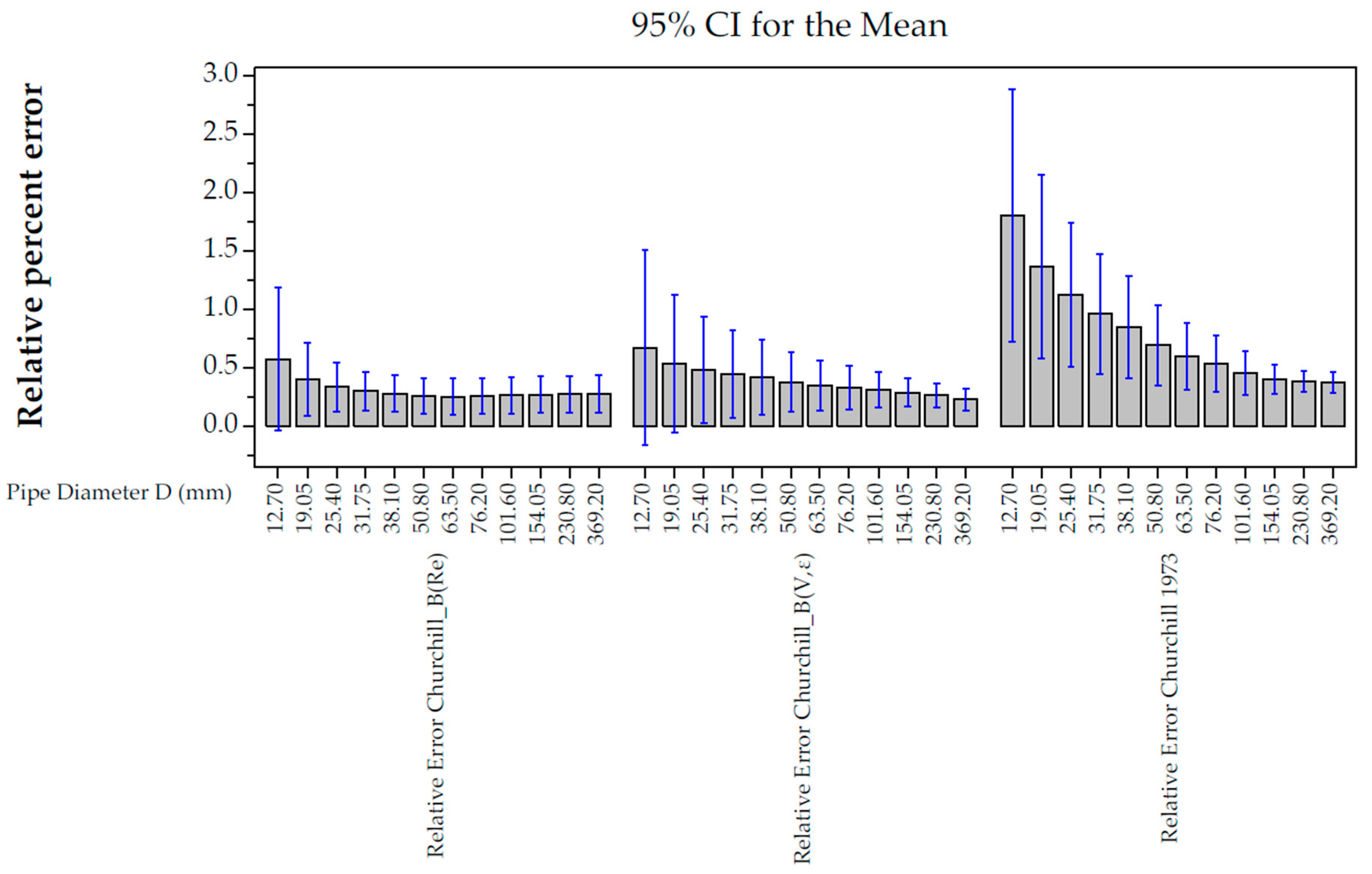
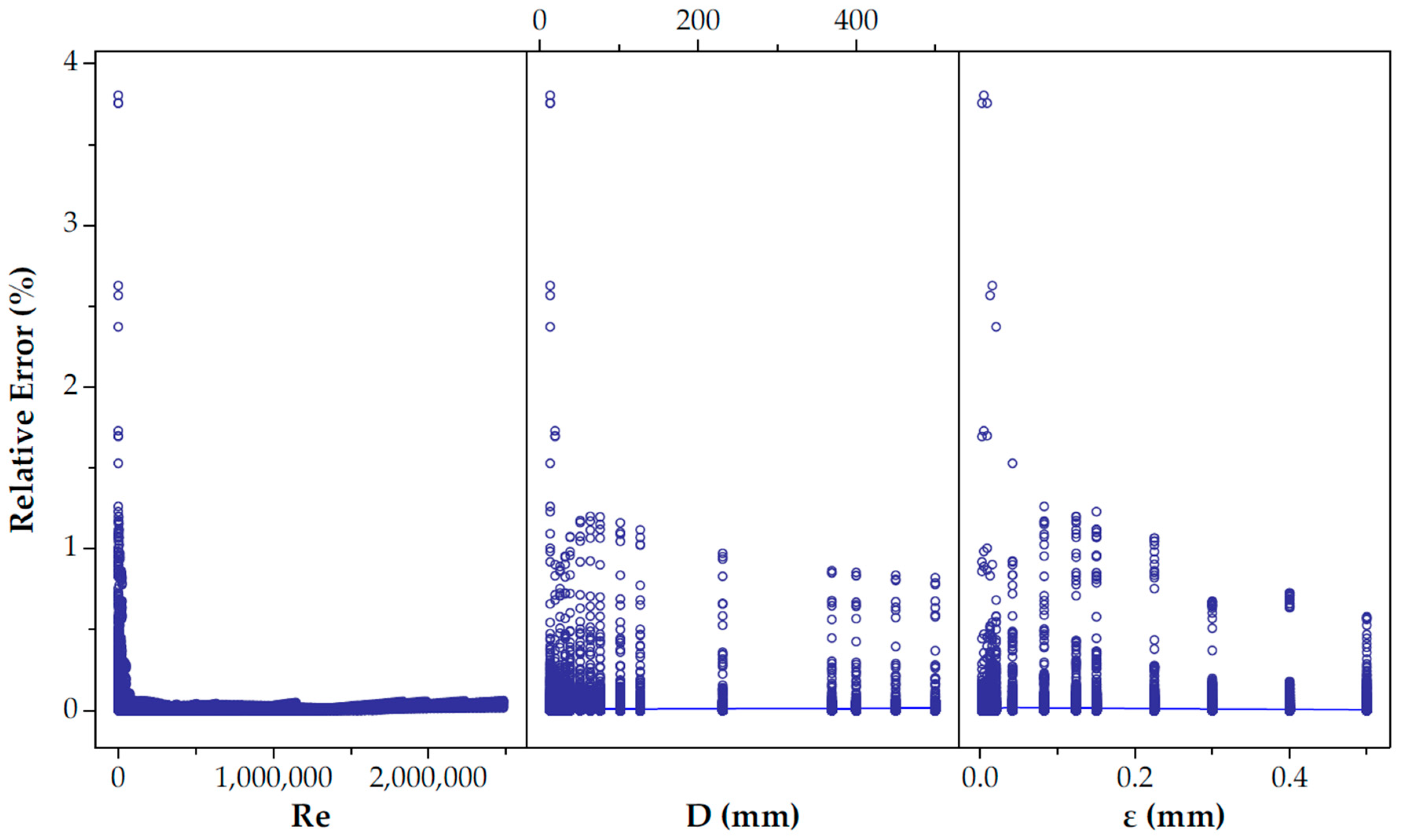
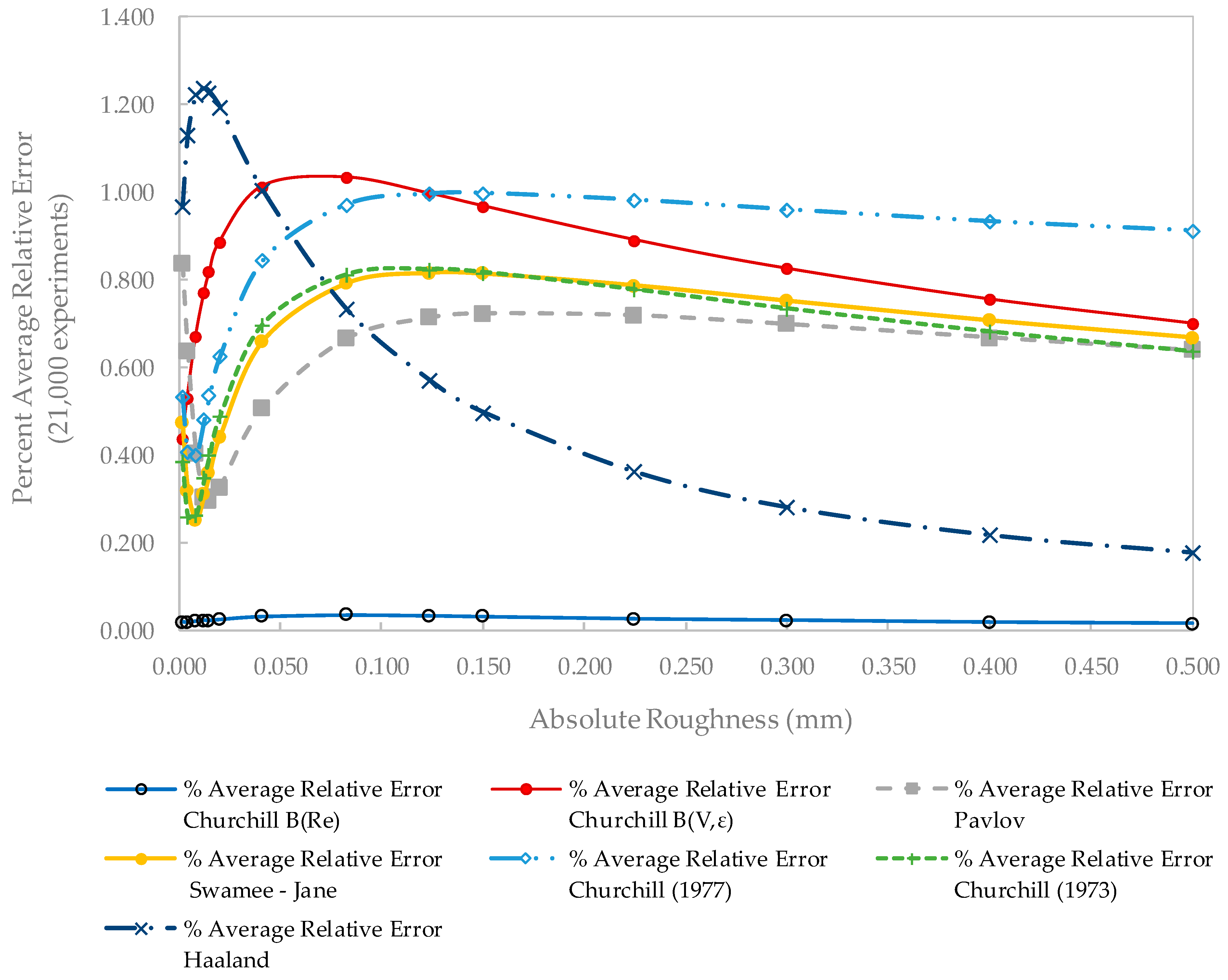
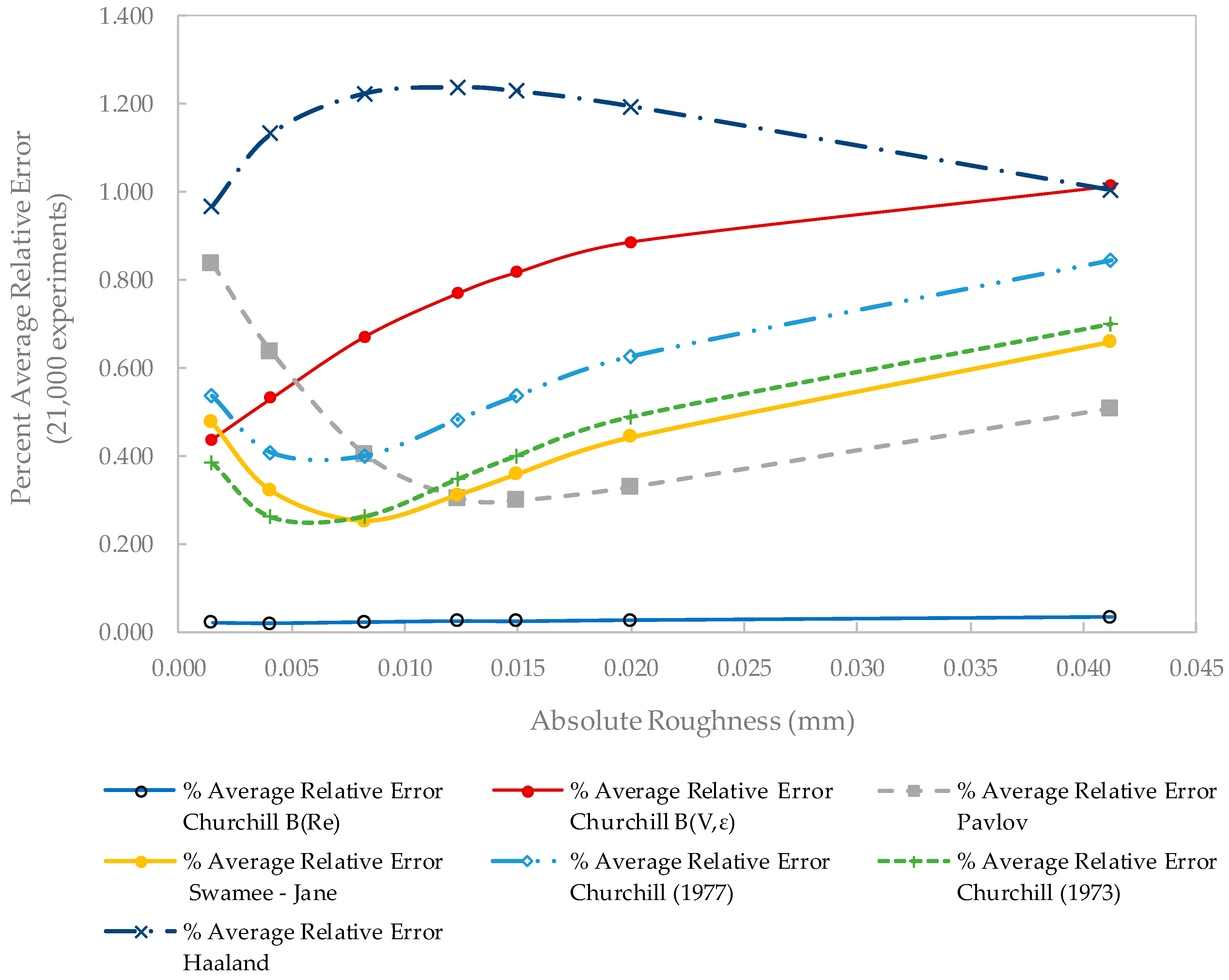
3.1.1. Relative Errors

The MRE for Churchill B(Re) is 0.0253%, while for Churchill B(V,ε), it is 0.8066%, indicating that the average relative error for Churchill B(Re) is more than 30 times smaller than that of Churchill B(V,ε) in calculating the friction factor f. Moreover, the standard deviation of the relative errors (SDRE) for Churchill B(Re) is 0.0916, which is less than a third of the standard deviation for Churchill B(V,ε) at 0.4654. This suggests that the relative errors for Churchill B(Re) are more consistent and less variable than those for Churchill B(V,ε) in calculating the friction factor f.

Figure 9 depicts the correlation between the percent average relative error and the absolute roughness of the Churchill B(Re) function (Equations (19) and (20)), compared to the Colebrook–White equation. The Churchill B(Re) function is grounded in 21,000 experiments, spanning 14 distinct roughness values, and it is a used empirical correlation for predicting the Darcy–Weisbach friction factor in pipe flow.

Figure 9 showcases the sixth-order regression model (dashed line), highlighting the robust association between the observed data and the fitted curve. The percent average relative error increases with roughness up to approximately 0.1 mm, after which it decreases steadily. The high R² value of 0.989 underscores the accuracy and reliability of the regression model in representing the experimental data, which is based on a sixth-order polynomial equation, for all values of roughness in mm, ranging from 0.0015 mm to 0.5000 mm. This behavior suggests that the model is robust in capturing the relationship between roughness and percent average relative error.

3.1.2. Absolute Errors

Evaluation of absolute errors across 240 test cases confirms the superior precision of the proposed equations. The absolute error of Churchill B(V,ε) is 1.5348 × 10⁻⁴, and that of Churchill B(Re) is 9.8737 × 10⁻⁵. Both values are lower than the absolute errors obtained using the models of Churchill [14] (7.6334 × 10⁻⁴), Churchill [28] (2.9111 × 10⁻⁴), Swamee and Jain [19] (2.7811 × 10⁻⁴), Haaland [18] (2.7239 × 10⁻⁴), Pavlov [48] (2.2675 × 10⁻⁴), and Barr [16] (2.1275 × 10⁻⁴).

This significant reduction in absolute error agrees with the advances reported by Brkić [30], who compiled various explicit equations that achieve absolute errors of the order of 10⁻⁵ or less.

Moreover, Genić et al. [8] noted the importance of minimizing both the absolute and relative errors when evaluating approximations to Colebrook–White.

Therefore, the new functions developed here represent a progress in terms of absolute precision over established alternatives. With its low relative error, this positions it as a viable and recommended explicit correlation for estimating the friction factor in engineering flow applications.

4. Discussion and Comparative Results

Figure 10 presents fitted line graphs comparing the calculated friction coefficient with the Churchill B(V,ε) and Churchill B(Re) functions, and that, calculated with the Colebrook–White equation, was solved by the Newton–Raphson method. Standard estimation errors (S) of 0.0004160 and 0.0002995, respectively, indicate a close proximity of data points to the fitted line, suggesting an excellent model fit. The coefficient of determination (R²) of 99.8% and 99.9% confirms a strong relationship between variables, while the adjusted coefficient of determination (R²(adj)) (99.8% and 99.9%) demonstrates the model´s robustness (see Figure 10a,d).

Figure 10a,d (Correlation Plot): Red points: These points indicate the observed data comparing the Churchill B(V,ε) function with the Colebrook-White function using the Newton-Raphson method. They show the direct relationship between the two methods. Blue line: This line represents the line of perfect correlation (y = x), showing the ideal case where the predicted values from both methods would be identical. The closer the red points are to this line, the stronger the correlation between the two methods. Figure 10b,e (Residual Plot): Red points: These represent the residuals, which are the differences between the observed values and the predicted values from the regression model. They are plotted against their corresponding percentiles to evaluate the goodness-of-fit. The blue line represents the theoretical normal distribution. The alignment of the red points along this line indicates how well the residuals follow a normal distribution. The residual plots for the friction factor calculated with the Churchill functions versus the friction factor determined with Colebrook–White and solved by Newton–Raphson (N-R) are calculated. In the normal probability graph, the universe of observations (N = 240) is included, with an Anderson Darling (AD) of 6.229 and 14.613, and p-Value < 0.005, indicating that there are significant tests against the normality of the residuals. All these statistical metrics suggest that the line of fit for the data is very effective. In this case, the values of the proposed function fit very closely to those of the comparative pattern.

4.1. Normal Probability Plot

The normal probability plots of the residuals in Figure 10b,e were constructed to assess the normality of the residuals and identify significant factors influencing the friction factor calculation. This plot is a graphical technique for normality testing, where the ordered residuals are plotted against the theoretical quantiles of a normal distribution [53].

The construction process of the normal probability plot involves the following steps: The residuals are ordered from smallest to largest. The cumulative probability for each residual is calculated. The probabilities are transformed to z-scores using the inverse of the standard normal cumulative distribution function. The ordered residuals are plotted on the x-axis against their corresponding z-scores on the y-axis. A reference line is added, representing the expected pattern if the effects were perfectly normally distributed.

In interpreting the plot, points that deviate substantially from the reference line indicate significant effects. These deviations are particularly important when they occur at the extremes of the distribution, as they represent effects larger than what would be expected from random variation alone.

Figure 10b presents the normal probability plot for the Churchill B(V,ε) function, which displays the residuals against a normal distribution. Key observations from this plot include a sample size (N) of 240 observations, an Anderson–Darling (AD) statistic of 6.329, and a p-value of less than 0.005, indicating significant evidence against the normality of residuals. The residuals predominantly lie between −0.001 and 0.001, with most data points closely aligned along the reference line, suggesting a systematic deviation from normality.

In the first case, there are approximately four points between residual values of 0.0005 to 0.004 that are close to the 99% percentile, indicating the presence of outliers or extreme values in the upper tail of the residual distribution. These residuals are much larger than what would be expected in a normal distribution, suggesting significant positive deviations in the model’s predictions for a small number of observations. The majority of residuals lie between −0.0005 and 0.0005, covering the central 98% of the distribution, indicating that the model’s predictions are fairly accurate for most observations, with low variability and high precision in the central part of the distribution. These findings suggest that the Churchill B(V,ε) model, while generally accurate, may systematically overpredict friction factors for a small subset of data points, particularly in laminar flow regimes.

Figure 10e presents the normal probability plot for the Churchill B(Re) function, displaying the residuals against a normal distribution, with a sample size (N) of 240 observations and an Anderson–Darling (AD) statistic of 14.613, as well as a p-Value < 0.005, indicating significant evidence against the normality of residuals.

There are two extreme outliers in the lower tail of the residual distribution, with one point at approximately −0.001 and another at −0.0036, both below the 1% percentile. These points represent significant negative deviations, indicating that for these few observations, the model significantly overestimated the friction factor. The majority of residuals are between −0.00025 and 0.0005, covering the central 98.5% of the distribution, indicating that the model’s predictions are highly accurate for most observations, with a slight positive bias. However, the presence of extreme negative outliers highlights areas where the model’s predictions are notably off. These findings suggest that the Churchill B(Re) model, while providing a generally accurate representation, may be subject to systematic overestimation for a small subset of data points, particularly in the lower tail of the residual distribution, particularly in laminar flow regimes.

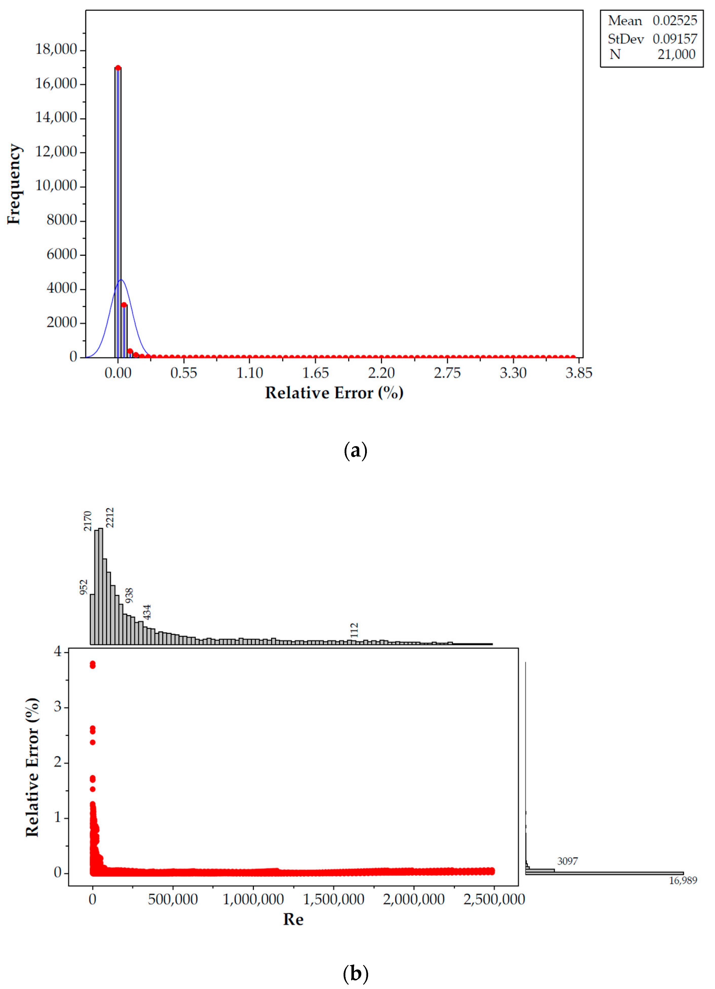
4.2. Histogram of the Residuals

The histogram of the residuals displays the distribution of residuals from the fitted model. Ideally, this histogram should resemble a bell-shaped curve, indicating that the residuals are normally distributed. In the 10b plot, the histogram appears to be somewhat symmetrical but not perfectly bell-shaped, suggesting some deviations from normality. The residuals are mostly centered around zero with a few outliers on both sides, indicating that most of the prediction errors are small, but there are some larger errors [54].

Figure 10c presents the residual histogram for the Churchill B(V,ε) function. The histogram displays a residual range of approximately −0.00075 to 0.00075, with a peak frequency exceeding 70 near zero. This indicates a clustering of residuals around the mean, suggesting potential negative bias in the model’s predictions. Negative residuals imply that the model overestimates friction factors compared to the Colebrook–White equation.

Figure 10f presents the residual histogram for the Churchill B(Re) function. The histogram displays a residual range of approximately −0.0003 to 0.0006, with a peak frequency exceeding 100 near zero. This indicates a clustering of residuals around the mean, suggesting potential positive bias in the model’s predictions. Positive residuals imply that the model underestimates friction factors compared to the Colebrook–White equation.

In Figure 11, a matrix of graphs is presented, which provides a view of the relationships between each pair of functions of interest. In this case, on the Y-axis of the matrix, the results of the friction coefficient calculation with Churchill B(V,ε) and Churchill B(Re) are located. And on the X-axis of the matrix, the results of the friction factor with the Churchill [14], Churchill [28], and Colebrook–White calculated by Newton–Raphson methods are shown.

In the matrix of Figure 11, the individual relationships of each function Y with each function X are presented. The strongest correlations are observed between the Churchill B(V,ε) function (Y) and Churchill model of 1973 (X), as well as between the Churchill B(Re) function (Y) and the Colebrook–White equation, solved using Newton–Raphson (X). However, discrepancies are noted in other comparisons, with more pronounced differences evident in the f_D Churchill [14] model. This visual analysis provides valuable details on the relationships and behaviors of the variations in the calculated friction factors.

4.3. Error Comparison

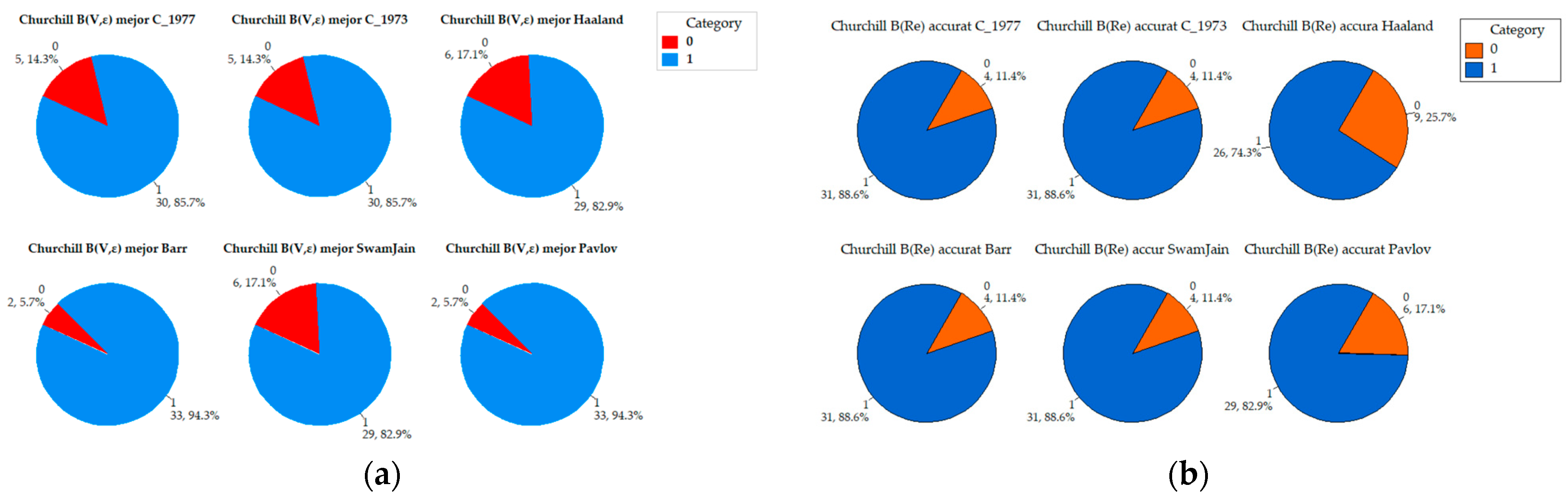
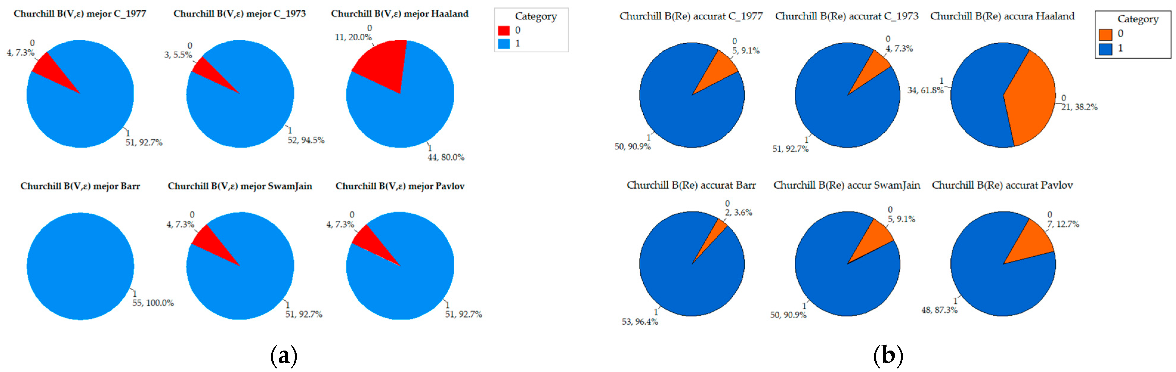
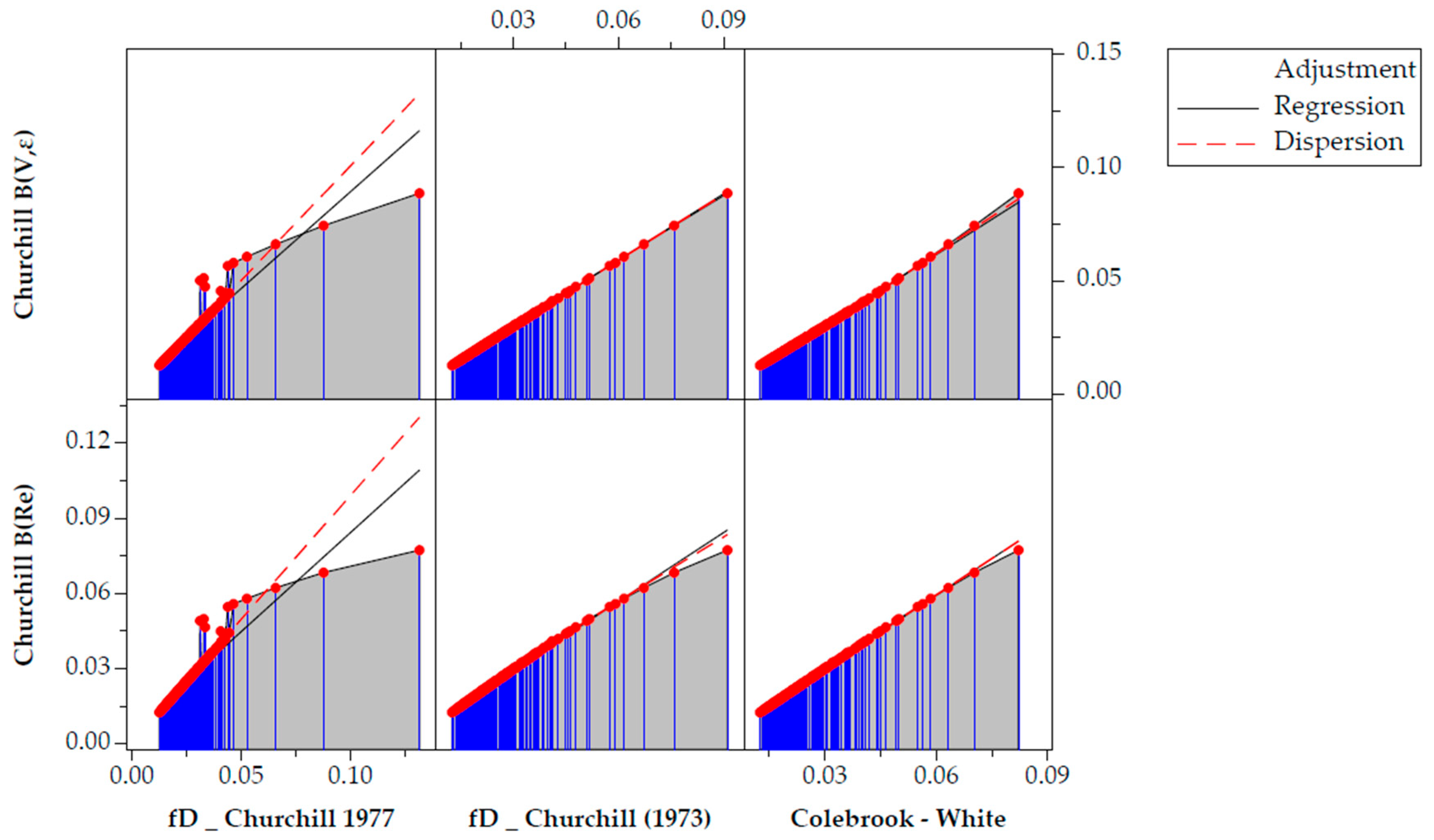
4.3.1. Absolute Error Comparison for Churchill B(V,ε) Function

Figure 12 presents an individual value plot that illustrates the absolute errors in friction-factor estimations using the Churchill B(Re) function, Churchill B(V,ε) function, and Churchill [14] models, all compared to the reference value obtained from the Colebrook–White equation using the Newton–Raphson method. The plot includes 95% confidence intervals for the mean, providing a detailed comparison of the error distributions across various pipe diameters.

The individual value plot (Figure 12) presents the absolute errors of three different models: Churchill B(Re), Churchill B(V,ε), and Churchill [28], plotted against the pipe diameter (D) in millimeters, with a 95% confidence interval (CI) for the mean.

As can be seen in Figure 12, the errors are grouped according to the 12 diameters studied for the 240 test cases. It is noticeable that the smallest absolute error corresponds to the Churchill functions, followed by Churchill [28] with a higher error, which shows the largest errors in the boxes by diameter, especially for 12.70 mm, 19.05 mm, 25.40 mm, and 31.75 mm. In contrast, the differences between errors are smaller for diameters of 230.80 mm and 369.20 mm. As the pipe diameter increases, the error distribution tends to narrow, suggesting a reduction in error variability for larger diameters.

The absolute errors for the newly proposed functions demonstrate a marked improvement in consistency and lower variability across all pipe diameters. The plot shows that the 95% CI for the mean is narrower for the new function, particularly for smaller diameters, indicating a more reliable and precise prediction of the friction factor.

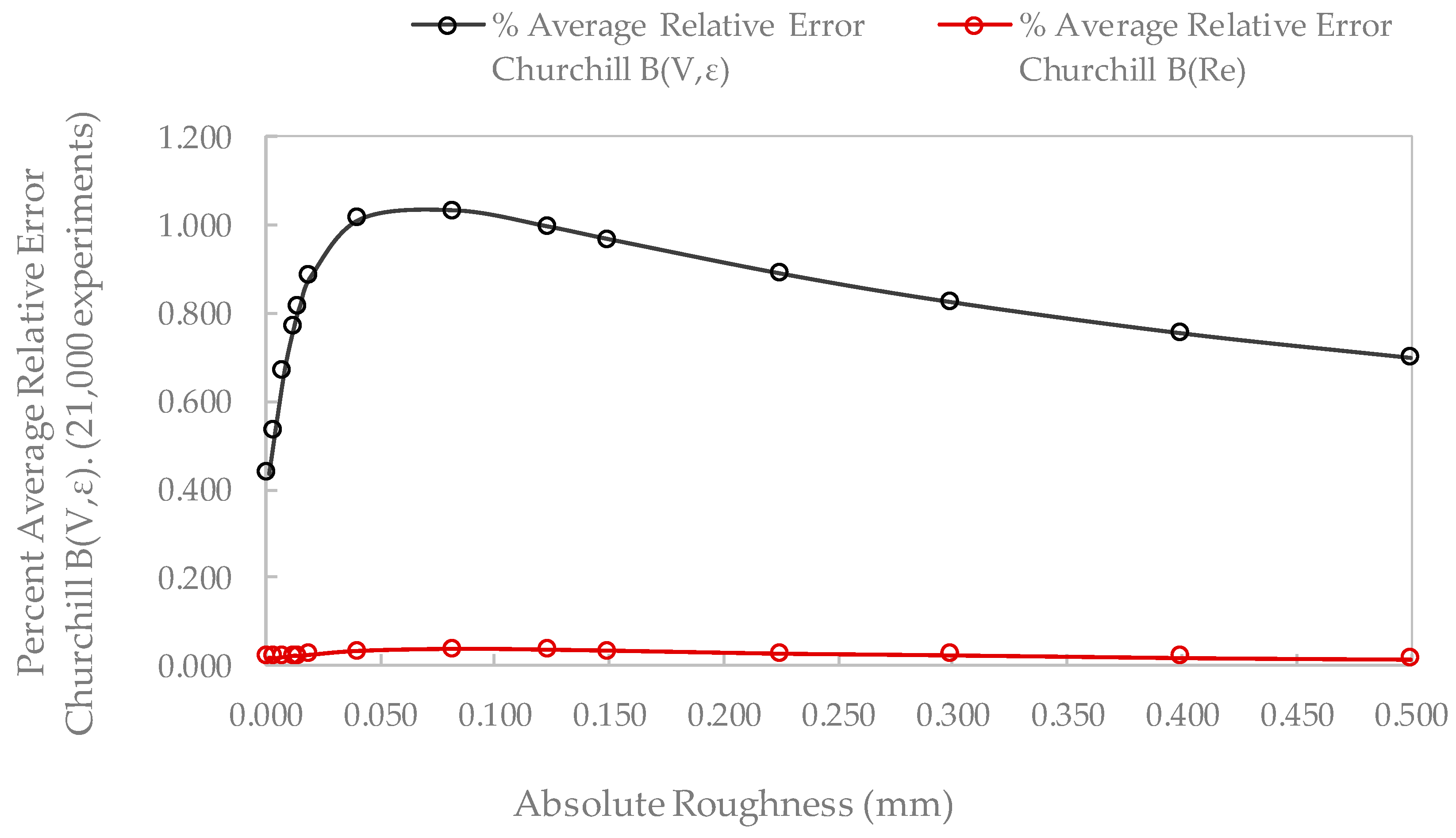
4.3.2. Relative Error Comparison for Churchill B(Re) Function

Figure 13 presents an individual value plot comparing relative percentage errors in friction-factor predictions between the Churchill B(Re), B(V,ε), and Churchill [14] models against the Colebrook–White equation (Newton–Raphson). The plot incorporates 95% confidence intervals for mean errors, enabling a detailed analysis of error distributions across varying pipe diameters.

Figure 13, incorporating confidence intervals, reveals varying degrees of accuracy across different pipe diameters. Each bar represents the 95% confidence interval for the mean relative error at each diameter and for each model. The “whiskers” indicate the data dispersion around the mean. The two models proposed in this study, Churchill B(Re) and B(V,ε), exhibit generally lower relative errors than Churchill’s model [28].

Figure 14 depicts the distribution of the relative error percentages when comparing the Churchill B(Re) function to the Colebrook–White equation, plotted against the Reynolds number (Re), pipe diameter (D), and absolute roughness (ε). This analysis provides insight into the variability and accuracy of the Churchill B(Re) approximation across different experimental conditions (based on 21,000 test cases).

Figure 14 presents the relative error distribution of the Churchill B(Re) function compared to the Colebrook–White method under various hydraulic conditions. The left subplot shows a pattern of relative errors below 1% across most Reynolds numbers, with errors decreasing as the Reynolds number increases, indicating a higher accuracy at higher Reynolds numbers.

The central subplot shows that the relative error varies across different pipe diameters, with higher errors at smaller and intermediate diameters, suggesting dependence on flow regimes and transition effects. This highlights the importance of considering these factors when applying the Churchill B(Re) function.

The right subplot reveals a correlation between higher absolute roughness values and increased relative error, indicating the Churchill B(Re) function’s sensitivity to surface roughness and potential for less accurate predictions on rougher surfaces.

Figure 15 illustrates the distribution of relative error percentages when comparing the Churchill B(Re) function to the Colebrook–White equation, plotted against the Reynolds number (Re). This figure includes a histogram of the frequency distribution of relative errors, accompanied by a probability density function (PDF), providing a statistical overview of the errors’ dispersion and central tendency. The comprehensive view highlights the error characteristics across different flow conditions.

Figure 15a demonstrates that the majority of relative errors are concentrated around 0%, with a mean error of 0.02525% and a standard deviation of 0.09157% when comparing the Churchill B(Re) function to the Colebrook–White equation.

The results demonstrate the Churchill B(Re) function’s reliability compared to Colebrook–White, with a high precision indicated by the skewness towards minimal error in the PDF overlay.

The sharp peak at the low error range suggests that the Churchill B(Re) function closely approximates the Colebrook–White equation for most experimental conditions. However, the presence of outliers with errors up to 3.85% highlights occasional discrepancies that may arise due to specific combinations of flow parameters and roughness effects, particularly when the flow regime is laminar, where the highest relative errors between Churchill B(Re) and Colebrook–White occur.

Figure 15b illustrates a distinct pattern in the relative error distribution with respect to the Reynolds number (Re). The scatter plot reveals that relative errors are predominantly below 1% for most Reynolds numbers, with a noticeable concentration of minimal errors as Re increases. This indicates enhanced accuracy of the Churchill B(Re) function at higher Reynolds numbers. The histogram above the scatter plot further emphasizes the frequency of these errors, showing that the majority are concentrated in the lower error range, with 16,989 instances near 0% and only 3097 slightly above 0.025%. This pattern suggests robust performance of the Churchill B(Re) function under various flow conditions, while the few higher errors at low Reynolds numbers highlight specific conditions where discrepancies may occur. The figure underscores the high precision and reliability of the Churchill B(Re) function, with most relative errors being minimal and well within acceptable limits. Additionally, it is confirmed that for laminar flow regimes, relative errors increase.

4.4. Statistical Significance

The narrower 95% confidence intervals (CI) for the mean absolute error of the new function compared to both Churchill [14] and Churchill [28] models highlight the enhanced precision of the proposed modification. The reduced error variability suggests that the new functions, Churchill B(Re) and Churchill B(V,ε), offer a more robust and accurate estimation of the friction factor across a wide range of pipe diameters, from 12.70 mm to 369.20 mm.

An analysis of the absolute errors and their corresponding 95% confidence intervals indicates that the new functions, Churchill B(Re) and Churchill B(V,ε), significantly improve the accuracy and reliability of friction factor calculations compared to the original Churchill [14] and Churchill [28] models. This enhancement is particularly evident at smaller pipe diameters, where the new functions exhibit substantially lower error variability and narrower confidence intervals.

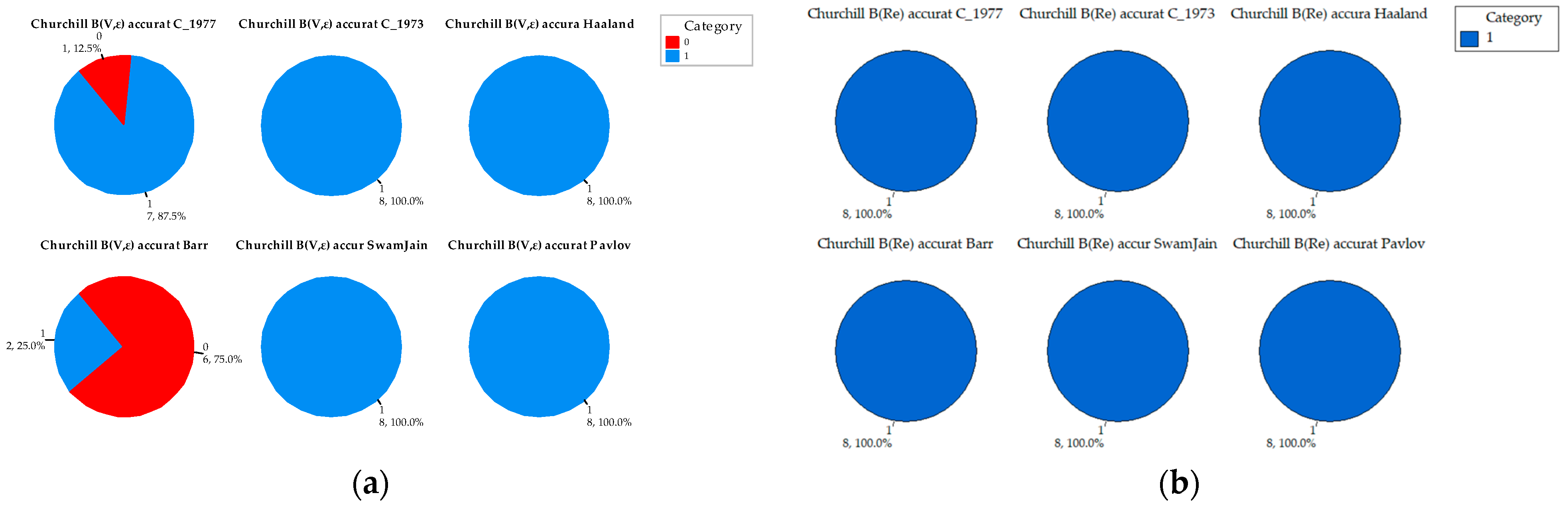
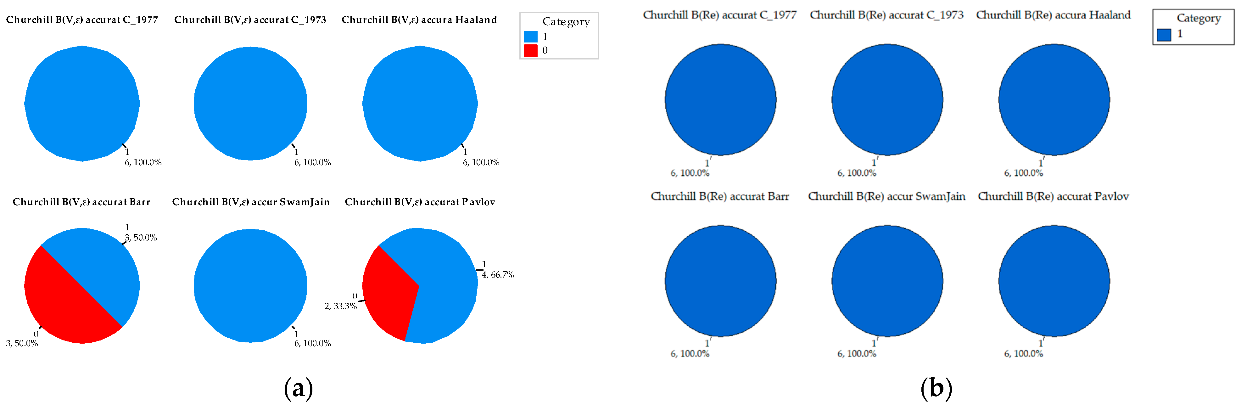
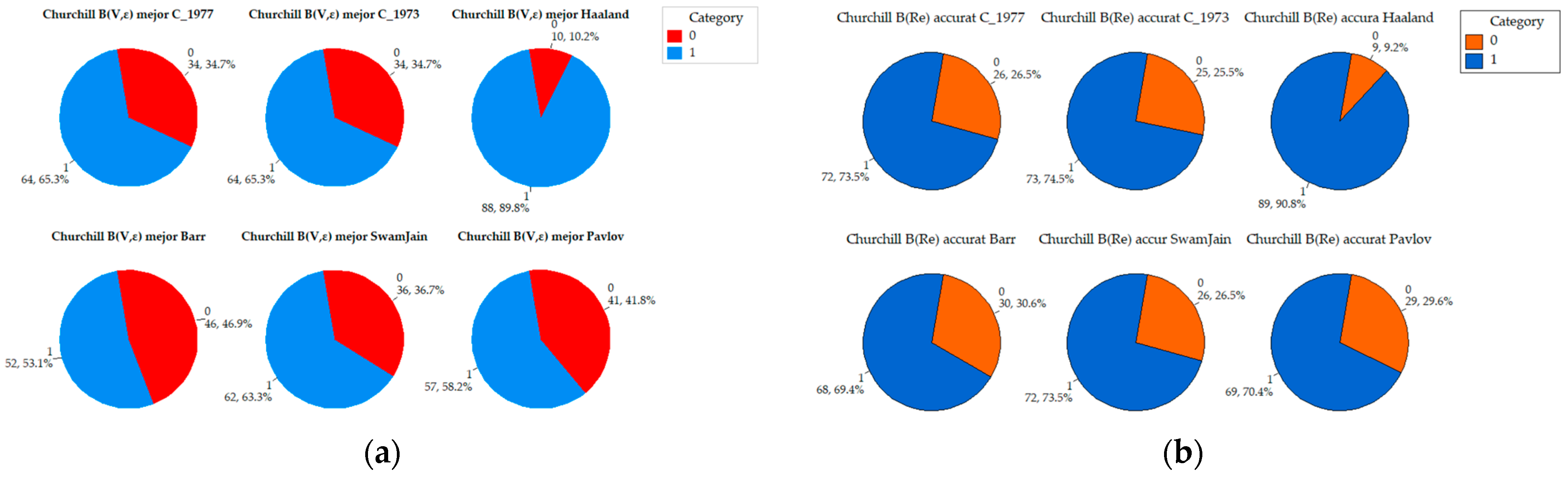
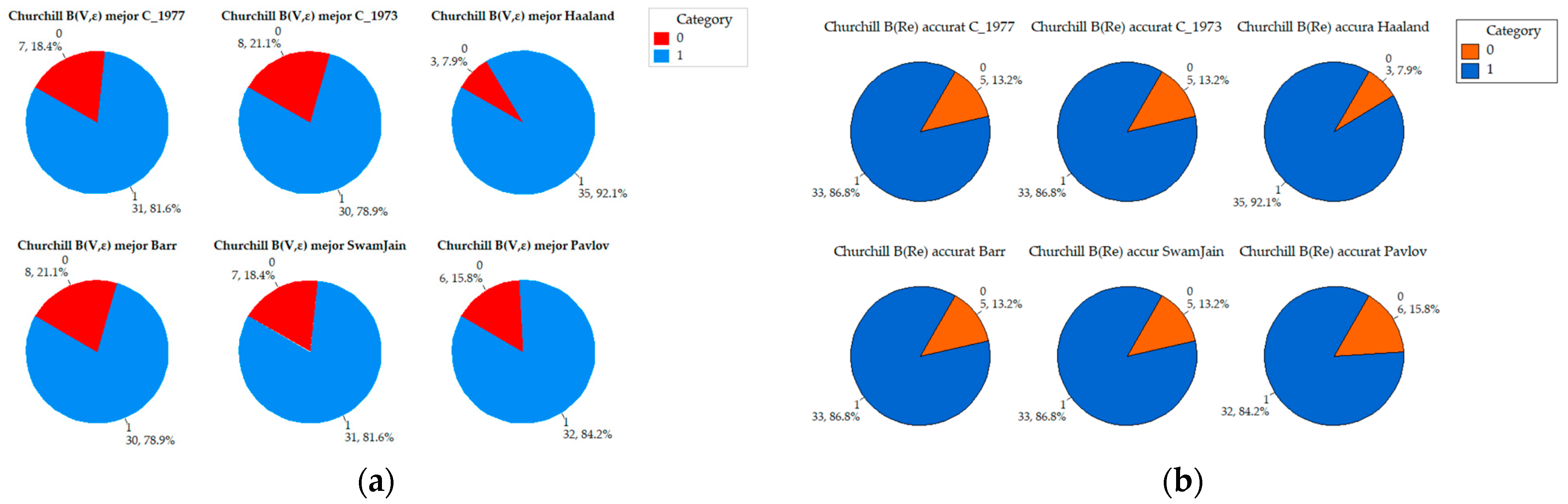
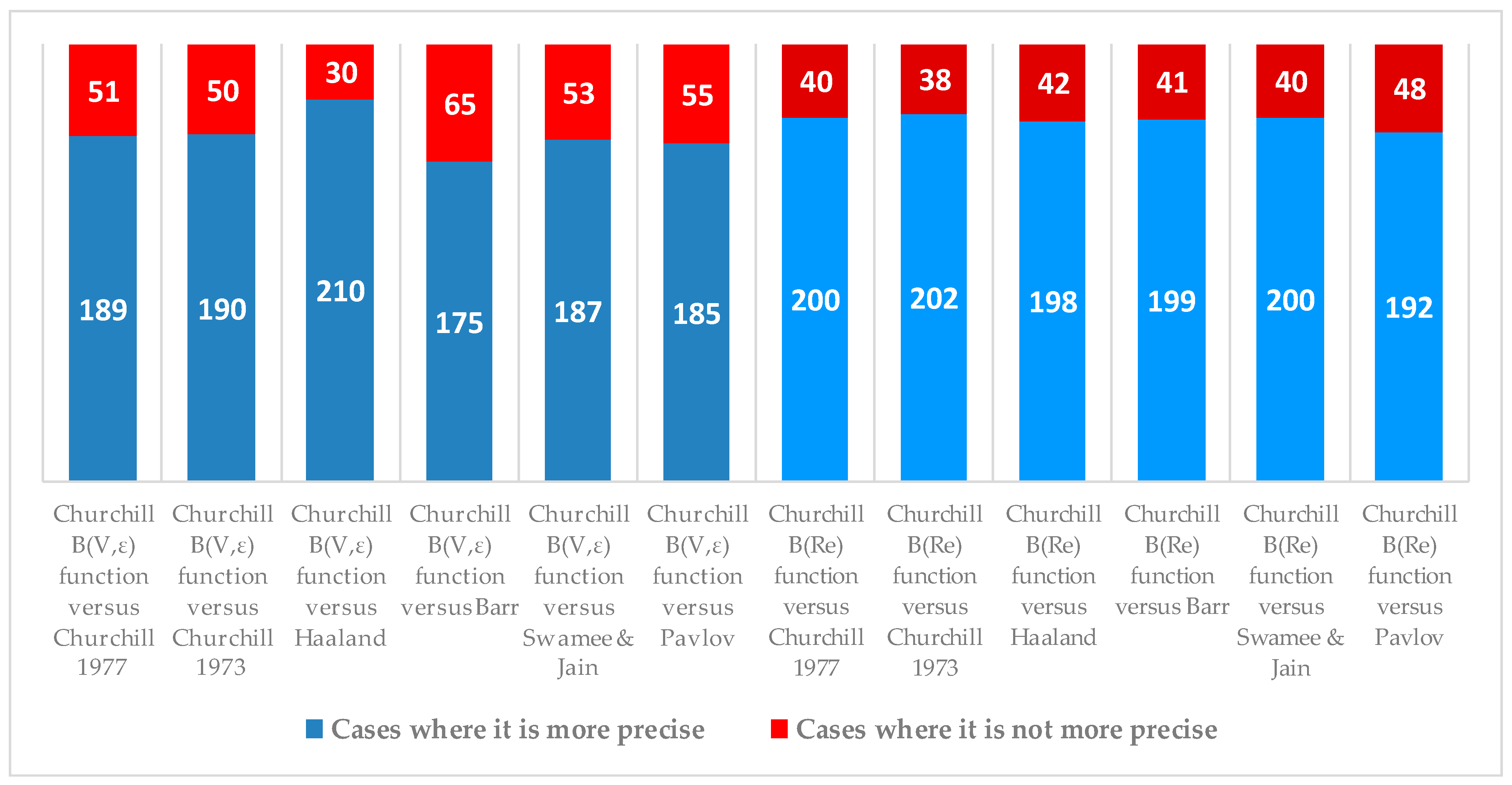
4.5. Analysis of Precision of the Churchill B(V,ε) Function in Comparative Cases

Figure 16 shows the results of the comparative analysis between the studied calculation methods. It highlights the cases in which the Churchill B(V,ε) function demonstrated greater precision than other reference models, including Churchill [14], Churchill [28], Haaland, Barr, Swamee and Jain, and Pavlov, all compared to the Colebrook–White method solved by Newton–Raphson (see Appendix A).

Each bar in the graph represents the total number of cases evaluated (N = 240). The lower section (blue) represents the number of cases where the Churchill B(Re) and Churchill B(V,ε) functions exhibited improved precision, as evidenced by a lower percentage error compared to the reference method. Conversely, the upper section (red) represents the number of cases where the Churchill functions did not demonstrate enhanced precision.

Table 3. Average relative error percentages of Churchill B(Re) and B(V,ε) functions vs. Colebrook–White equation.

Pipe Roughness ε (mm)	% Average Relative Error Churchill B(Re)	% Average Relative Error Churchill B(V,ε)
0.001500	0.019808	0.437443
0.004125	0.018866	0.531191
0.008250	0.021176	0.671271
0.012375	0.023488	0.769550
0.015000	0.023097	0.817256
0.020000	0.025254	0.885935
0.041250	0.032443	1.013247
0.082500	0.036022	1.033179
0.123750	0.034340	0.996127
0.150000	0.032512	0.967613
0.225000	0.027243	0.889976
0.300000	0.023956	0.824762
0.400000	0.019154	0.754921
0.500000	0.016149	0.699515

presents the average relative error percentages generated from 21,000 experiments, comparing the two proposed functions, Churchill B(Re) and Churchill B(V,ε), to the Colebrook–White equation. Each function was evaluated through 1500 experiments for each of the 14 different values of pipe roughness. A visual representation of these results can be found in Figure 16.

Figure 17 provides a detailed analysis of the percent average relative error in the pre-dicting friction factor using the Churchill B(Re) function and the Churchill B(V,ε) function to the Colebrook–White equation across various levels of absolute roughness. The graph highlights that the Churchill B(Re) function exhibits consistently lower errors compared to the Churchill B(V,ε) function.

The error for the Churchill B(Re) function remains below 0.037% across all tested roughness values, demonstrating its high precision and reliability. Conversely, the Churchill B(V,ε) function shows a significant increase in error, reaching up to 1.0%, indicating lower accuracy under similar conditions.

Within the tested Reynolds number range (with a minimum of Re = 631), Figure 18a,b reveals that the maximum relative percentage errors occur at the lowest Reynolds number evaluated across the 21,000 test cases.

Figure 18a reveals that the relative error is generally lower than that observed in Figure 18b, typically remaining below 1.00%. Data points corresponding to lower roughness values (ε ≤ 0.015 mm) exhibit exceptionally low relative errors, frequently below 0.75%. However, a slight trend of increasing relative error is noticeable for Reynolds numbers below 650 and for lower relative roughness values.

As depicted in Figure 18b, the relative error remains generally below 5% for low relative roughness values (ε/D), indicating a strong agreement between the two methods under smooth flow conditions. However, a marked increase in relative error is observed with increasing roughness, culminating in a 20% discrepancy at ε = 0.50 mm. This trend suggests a significant decline in the predictive accuracy of the Churchill B(V,ϵ) equation under high roughness conditions and in laminar flow regimes with Reynolds numbers below 650.

The analysis of percent average relative errors for various explicit friction factor methods against the Colebrook–White equation across a wide range of absolute roughness values is fundamental for understanding their accuracy and reliability. Figure 19 compares the methods over roughness values from 0.0015 mm to 0.5000 mm, providing a comprehensive evaluation of their performance.

As depicted in Figure 19, the Churchill B(Re) method exhibits a minimal error across all roughness values, thereby emerging as the most reliable among the evaluated explicit methods. While the performance of other methods tends to improve with increasing roughness, none can match the consistent accuracy of the Churchill B(Re) method.

A detailed examination of explicit friction factor methods at low roughness levels is essential for precision in hydraulic calculations where minimal roughness is common. Figure 20 focuses on the percent average relative errors of these methods for roughness values from 0.0015 mm to 0.04125 mm.

In this study, the Churchill B(Re) method proves to be the most reliable for all roughness scenarios, maintaining minimal error. Other methods, such as the Churchill model of 1973 and Swamee–Jain methods, exhibit moderate performance, while the Haaland method shows higher relative errors up to 0.04125 mm of roughness, although it presents lower errors from 0.1 mm to 0.5 mm. The Pavlov method presents low relative errors starting from 0.012375 mm. This focused analysis underscores the importance of selecting the most precise method, such as the Churchill B(Re) method, for hydraulic calculations using explicit applications.

Comparative Analysis

The comparative analysis of the Churchill B(Re) and B(V,ε) functions highlights their respective strengths and weaknesses. The Churchill B(Re) function excels in accuracy, offering minimal relative errors for a broad range of roughness values. However, this comes with the drawback of higher computational demands, as it requires multiple factors derived from detailed tables or regression functions. Conversely, the Churchill B(V,ε) function simplifies implementation by depending only on velocity and roughness, making it advantageous in situations where velocity is a consistent and known variable. Despite this ease of use, it falls short in precision, especially under conditions of significant roughness, resulting in comparatively higher relative errors (see

Table 4. Comparative analysis of advantages and disadvantages: Churchill B(V,ε) vs. Churchill B(Re) functions.

Model	Advantages	Disadvantages
Churchill B(Re) Function	High precision across a wide range of roughness Maintains low relative errors (<0.02%) for small to medium roughness values.	Greater computational complexity due to the need to read multiple factors (F, G, H, J, K, M) from a table or regression functions generated for each factor based on roughness.
Churchill B(V,ε) Function	Lower computational complexity, relying only on velocity and roughness. Easier to implement in applications where velocity is a known and constant parameter.	Lower precision compared to Churchill B(Re), especially in high roughness conditions. Higher relative errors (>0.02%) for certain roughness ranges.

).

In summary, although the Churchill B(V,ε) function offers simplicity and ease of implementation, its precision is inferior compared to the Churchill B(Re) function proposal. The latter exhibits superior robustness and significantly lower relative errors across a wide range of roughness, albeit at the cost of increased computational complexity. The choice between these models depends on the balance between the need for precision and the simplicity of implementation in specific applications.

5. Conclusions

The novel Churchill B(Re) and B(V,ε) functions, based on the preceding equation of Churchill [28], provide a robust and computationally efficient alternative to the Colebrook–White equation for determining friction factors in piping systems. These functions exhibit exceptional agreement with the established Colebrook–White correlation in terms of both absolute and relative error. Consequently, they enable more precise estimations of friction losses, leading to improved predictions of fluid flow behavior and optimized system design.

The development of these functions was made possible by the use of GRG nonlinear optimization, which enabled the creation of an improved Churchill equation with enhanced accuracy in predicting friction factors. This optimized equation offers a practical and precise alternative to the Colebrook–White equation, facilitating its application in hydraulic engineering.

The functions developed in this study exhibit superior precision in estimating the friction factor compared to the methods of Churchill (1977 [14] and 1973 [28]), Haaland, Barr, Swamee and Jain, and Pavlov. Of the 240 test cases, the Churchill B(V,ε) function demonstrates higher accuracy in 79% of cases compared to the Churchill [14] and Churchill [28] methods, 88% compared to Haaland, 73% compared to Barr method, 78% compared to Swamee and Jain method, and 77% compared to Pavlov. Similarly, the Churchill B(Re) function is more accurate in 83% of the cases compared to Churchill [14], 84% compared to Churchill [28], 83% compared to Haaland, Barr, and Swamee and Jain, and 80% compared to Pavlov.

The proposed Churchill B(Re) and Churchill B(V,ε) models demonstrate significantly improved accuracy compared to the original Churchill equation, with mean relative errors (MRE) of 0.025% and 0.807%, respectively, and mean absolute errors (MAE) of 0.0008% and 0.0154%, respectively. The Churchill B(Re) model shows higher accuracy across a range of roughness values, making it more reliable for precise friction-factor calculations. The Churchill B(Re) function demonstrates superior precision compared to Churchill B(V,ε). The Churchill B(Re) model shows higher accuracy across a range of roughness values, making it more reliable for precise friction factor calculations. Notably, dividing the average relative error of Churchill B(V,ε) by that of Churchill B(Re) yields an overall ratio of 32.41, indicating that Churchill B(Re) is significantly more precise. Specifically, for an epsilon of 0.0015, Churchill B(Re) is 22.08 times more precise than Churchill B(V,ε), and for an epsilon of 0.5000, Churchill B(Re) is 43.32 times more precise. The trade-off for this accuracy is greater computational complexity, as it requires the consideration of multiple factors derived from tables or regression functions specific to roughness.

Conversely, the Churchill B(V,ε) function, while easier to implement due to its reliance solely on velocity and roughness, sacrifices some degree of precision. This is especially noticeable under conditions of high roughness, where it results in higher relative errors compared to the Churchill B(Re) function.

The development of simple and accurate explicit equations, such as the one presented in this review study, facilitates the calculations involved in internal flow engineering applications related to pressure loss. Additionally, this simplification also has an educational value by allowing chemical, hydraulic, or pressure flow engineering students to understand and effectively apply concepts related to the friction factor in practical situations.

While the Churchill B(V,ε) function offers significant educational and computational advantages, the Churchill B(Re) function stands out for its higher precision. This dual insight provides a comprehensive understanding of the trade-offs involved, guiding the selection of the appropriate model based on the specific requirements of the hydraulic system being analyzed. This study thus contributes valuable knowledge to both the academic–scientific community and practicing engineers, introducing new equations for the explicit estimation of the friction factor and enhancing the understanding and application of fluid flow concepts in piping systems.

5.1. Limitations of the Study

This study offers valuable insights into the improved precision of the Churchill B(V,ε) and Churchill B(Re) functions for friction-factor estimation. However, some limitations should be considered when interpreting the results:

5.1.1. Sample Size and Flow Conditions

The analysis relied on a dataset of 240 cases, which were validated through 21,000 experiments. This can be considered relatively small compared to the vast spectrum of flow conditions encountered in real-world engineering applications.

This limitation restricts the generalizability of the findings to the entire potential scenarios.

5.1.2. Fluid Properties

The current study focused solely on incompressible fluids. However, the impact of fluid compressibility on the friction factor can be significant in high-pressure or high-velocity applications. Additionally, non-Newtonian fluids (fluids that do not exhibit a constant viscosity) were not considered.

5.1.3. Comparison Scope

This study compared the Churchill B(V,ε) and Churchill B(Re) functions with six commonly used methods. While valuable, this might be a limited number for a comprehensive evaluation.

5.2. Future Work

The present study offers valuable insights into the Churchill B(V,ε) and Churchill B(Re) functions, paving the way for further research to enhance its understanding and applicability. Here are some promising directions for future exploration:

5.2.1. Expand the Dataset and Flow Conditions

A comprehensive review of existing literature could identify a broader range of flow conditions, including variations in pipe diameter, roughness, Reynolds number, and fluid properties. Utilizing this expanded dataset would allow for a re-evaluation of the Churchill B(V,ε) and Churchill B(Re) function’s performance and assessment of its generalizability to a wider spectrum of real-world scenarios.

5.2.2. Explore Fluid Property Effects

Investigating the applicability of the Churchill B(V,ε) and Churchill B(Re) functions to compressible fluids could involve incorporating relevant thermodynamic properties into the model. Extending the analysis to non-Newtonian fluids could be achieved by considering their unique viscosity characteristics and developing appropriate modifications to the function.

5.2.3. Evaluating the Practicality and Impact of Incorporating the New Churchill B(V,ε) and Churchill B(Re) Expression in WDS Simulation Software (in the Most Current Version Available at the Time of the Future Evaluation)

A critical aspect of future research involves investigating the feasibility of incorporating the new B(V,e) and B(Re) expression into widely used open-source WDS simulation software like EPANET 2.2, facilitating wider adoption and fostering further development. This involves developing appropriate integration methods and evaluating the impact on user workflows and computational demands [55]. Once integrated within EPANET, a comprehensive comparison of the new expression with existing methods within the software is necessary. This analysis should evaluate the impact of Churchill B(V,e) and Churchill B(Re) on simulation accuracy, convergence behavior of solution algorithms, and potential computational overhead.

5.2.4. Broaden the Comparison Scope

A more extensive comparison of the Churchill B(V,ε) and Churchill B(Re) functions with a wider range of existing friction factor estimation methods could be conducted. Evaluating the performance of these methods under different flow conditions and fluid properties could help identify the most suitable approaches for specific applications.

5.2.5. Experimentally Validate and Explore Advanced Techniques

To validate the new friction factor equation, it is crucial to compare it against experimental loss of charge data obtained through high-precision instrumentation [56]. This can be accomplished by fitting pressures using experimental data and adjusting the model roughness until there is agreement between calculated and observed values.

Additional experimental validations of the proposed new equation could be planned, utilizing experimental data across various flow conditions. Validation of the new friction factor equation against experimental loss of charge data in pipes obtained through high-precision instrumentation could be a valuable step.

References

1. Silverio, N.; Benavides-Muñoz, H.B. Determinación de pérdidas de carga en accesorios “k” de Sistemas Domiciliarios. Ecuadorian Sci. J. 2020, 4, 7–11. [Google Scholar] [CrossRef]
2. Paloka, E.M.; Pažanin, I. Effects of boundary roughness and inertia on the fluid flow through a corrugated pipe and the formula for the Darcy–Weisbach friction coefficient. Int. J. Eng. Sci. 2020, 152, 103293. [Google Scholar] [CrossRef]
3. Zierep, J.; Bühler, K. Principles of Fluid Mechanics: Fundamentals, Statics and Dynamics of Fluids; Springer Nature: Wiesbaden, Germany, 2022. [Google Scholar]
4. Kundu, P.K.; Cohen, I.M.; Dowling, D.R. Fluid Mechanics, 6th ed.; Academic Press: Cambridge, MA, USA; Elsevier: Amsterdam, The Netherlands, 2016; p. 922. [Google Scholar]
5. Wilkes, J.O. Fluid Mechanics for Chemical Engineers; Wilkes, J., Ed.; with contributions by Stacy G. Bike; Prentice Hall International Series in the Physical and Chemical Engineering Sciences; Prentice Hall PTR: Hoboken, NJ, USA, 1999; p. 599. [Google Scholar]
6. Colebrook, C.F.; White, C.M. Experiments on turbulent flow in smooth pipes with particular reference to the transition region between smooth and rough pipe laws. Proc. R. Soc. Lond. A Math. Phys. Sci. 1937, 161, 391–418. [Google Scholar]
7. Moody, L.F. Friction factors for pipe flow. Trans. ASME 1944, 66, 671–684. [Google Scholar] [CrossRef]
8. Genić, S.; Aranđelović, I.; Kolendić, P.; Jarić, M.; Budimir, N.; Genić, V. A review of explicit approximations of Colebrook’s equation. FME Trans. 2011, 39, 67–71. [Google Scholar]
9. Muzzo, L.E. Análise Comparativa de Correlações para o Fator de Atrito em Condutas. Ph.D. Thesis, Instituto Politecnico de Braganca (Portugal), Bragança, Portugal, 2019. [Google Scholar]
10. Brkić, D.; Praks, P. Discussion of Approximate Analytical Solutions for the Colebrook Equation by Ali R. Vatankhah. J. Hydraul. Eng. 2020, 146, 07019011. [Google Scholar] [CrossRef]
11. Plascencia, G.; Díaz–Damacillo, L.; Robles-Agudo, M. On the estimation of the friction factor: A review of recent approaches. SN Appl. Sci. 2020, 2, 163. [Google Scholar] [CrossRef]
12. NACA. Laws of Flow in Rough Pipes; Technical Memorandum 1292. Translation of Strömungsgesetze in rauhen Rohren. VDI Forschungsheft 361. Beilage zu Forschung auf dem Gebiete des Ingenieurwesens. 1933. 1950. TM 1292; National Advisory Committee for Aeronautics: Washington, DC, USA, 1950. [Google Scholar]
13. Wood, D.J. An explicit friction factor relationship. Civ. Eng. 1966, 36, 60–61. [Google Scholar]
14. Churchill, S.W. Friction factor equations span all fluid flow regimes. Chem. Eng. 1977, 84, 91. [Google Scholar]
15. Chen, N.H. An explicit equation for friction factor in pipe. Ind. Eng. Chem. Fundam. 1979, 18, 296–297. [Google Scholar] [CrossRef]
16. Barr, D.I.H. Solutions of the Colebrook-White function for resistance to uniform turbulent flow. Proc. Inst. Civ. Eng. 1981, 71, 529–536. [Google Scholar]
17. Churchill, S.W.; Chan, C. Improved correlating equations for the friction factor for fully turbulent flow in round tubes and between identical parallel plates, both smooth and naturally rough. Ind. Eng. Chem. Res. 1994, 33, 2016–2019. [Google Scholar] [CrossRef]
18. Haaland, S.E. Simple and explicit formulas for the friction factor in turbulent pipe flow. J. Fluids Eng.-Trans. ASME 1983, 105, 243. [Google Scholar] [CrossRef]
19. Swamee, P.K.; Jain, A.K. Explicit equations for pipe-flow problems. J. Hydraul. Div. 1976, 102, 657–664. [Google Scholar] [CrossRef]
20. Nurudin, A.S. Error Review of Single Iteration Explicit Approximations of Colebrook’s Equation. Selangor Sci. Technol. Rev. (SeSTeR) 2021, 5, 22–30. [Google Scholar]
21. Papaevangelou, G.; Evangelides, C.; Tzimopoulos, C. A new explicit relation for the friction factor coefficient in the Darcy–Weisbach equation. In Proceedings of the Tenth Conference on Protection and Restoration of the Environment, Corfu, Greece, 5–9 July 2010; Volume 166, pp. 5–9. [Google Scholar]
22. Salmasi, F.; Khatibi, R.; Ghorbani, M. A study of friction factor formulation in pipes using artificial intelligence techniques and explicit equations. Turk. J. Eng. Environ. Sci. 2012, 36, 121–138. [Google Scholar]
23. Bonakdari, H.; Zaji, A.H.; Shamshirband, S.; Hashim, R.; Petkovic, D. Sensitivity analysis of the discharge coefficient of a modified triangular side weir by adaptive neuro-fuzzy methodology. Measurement 2015, 73, 74–81. [Google Scholar] [CrossRef]
24. Bemani, A.; Kazemi, A.; Ahmadi, M.; Yousefzadeh, R.; Moraveji, M.K. Rigorous modeling of frictional pressure loss in inclined annuli using artificial intelligence methods. J. Pet. Sci. Eng. 2022, 211, 110203. [Google Scholar] [CrossRef]
25. Najafzadeh, M.; Shiri, J.; Sadeghi, G.; Ghaemi, A. Prediction of the friction factor in pipes using model tree. ISH J. Hydraul. Eng. 2018, 24, 9–15. [Google Scholar] [CrossRef]
26. Azizi, N.; Homayoon, R.; Hojjati, M.R. Predicting the Colebrook–White friction factor in the pipe flow by new explicit correlations. J. Fluids Eng. 2019, 141, 051201. [Google Scholar] [CrossRef]
27. Olivares, A.; Guerra, R.; Alfaro, M.; Notte-cuello, E.; Puentes, L. Experimental evaluation of correlations used to calculate friction factor for turbulent flow in cylindrical pipes. Rev. Int. Métodos Numér. Cálculo Diseño Ing. 2019, 35, 15. [Google Scholar] [CrossRef]
28. Churchill, S.W. Friction factor for laminar and turbulent flow of a fluid through a pipe. J. Fluid Mech. 1973, 52, 447–460. [Google Scholar]
29. Jain, A.K. Accurate explicit equation for friction factor. J. Hydraul. Div. 1976, 102, 674–677. [Google Scholar] [CrossRef]
30. Brkić, D. Review of explicit approximations to the Colebrook relation for flow friction. J. Pet. Sci. Eng. 2011, 77, 34–48. [Google Scholar] [CrossRef]
31. Zigrang, D.J.; Sylvester, N.D. A review of explicit friction factor equations. J. Energy Resour. Technol. 1985, 107, 280–283. [Google Scholar] [CrossRef]
32. Shacham, M. An Explicit Equation for Friction Factor in Pipe. Ind. Eng. Chem. Fundam. 1980, 19, 229–230. [Google Scholar] [CrossRef]
33. Fang, X.P. Hydraulics of Pressurized Flow. In Water Encyclopedia; Lehr, J.H., Keeley, J., Eds.; Surface and Agricultural Water; Wiley Interscience: New York, NY, USA, 2005; Volume 3, pp. 196–199. [Google Scholar]
34. Eck, B. Technische Stromungslehre. Springer-Verlag, 1973. Citado en: Cheng, N.-S. Simplified explicit equations for the Colebrook–White equation. J. Hydraul. Eng. 2011, 137, 1717–1719. [Google Scholar]
35. Serghides, T.K. Estimate friction factor accurately. Chem. Eng. 1984, 91, 63–64. [Google Scholar]
36. Sonnad, J.R.; Goudar, C.T. Turbulent flow friction factor calculation using a mathematically exact alternative to the Colebrook-White equation. J. Hydraul. Eng. 2006, 132, 863–867. [Google Scholar] [CrossRef]
37. Avci, A.; Karagoz, I. A novel explicit equation for friction factor in smooth and rough pipes. J. Fluids Eng. 2009, 131, 061203. [Google Scholar] [CrossRef]
38. Majid, N.; Nasser, T. Comparison of Explicit Relations for Calculating Colebrook Friction Factor in Pipe Network Analysis Using h-based Methods. Iran. J. Sci. Technol.-Trans. Civ. Eng. 2020, 44, 231–249. [Google Scholar] [CrossRef]
39. Brkić, D. New explicit correlations for turbulent flow friction factor. Nucl. Eng. Des. 2011, 241, 4055–4059. [Google Scholar] [CrossRef]
40. Asker, M.; Turgut, O.E.; Coban, M.T. A review of non-iterative friction factor correlations for the calculation of pressure drop in pipes. Bitlis Eren Univ. J. Sci. Technol. 2014, 4, 1–8. [Google Scholar]
41. Vatankhah, A.R. Approximate analytical solutions for the Colebrook equation. J. Hydraul. Eng. 2018, 144, 06018007. [Google Scholar] [CrossRef]
42. López-Silva, M.; Carmenates-Hernández, D.S.; Delgado-Hernández, N.; Chunga-Bereche, N. Explicit Pipe Friction Factor Equations: Evaluation, Classification, and Proposal. Rev. Fac. Ing. Univ. Antioq. 2024, 111, 38–47. [Google Scholar] [CrossRef]
43. Narciso, D.A.; Pistikopoulos, E.N. Novel solution strategies for multiparametric nonlinear optimization problems with convex objective function and linear constraints. Optim. Eng. 2024, 1–29. [Google Scholar] [CrossRef]
44. McWilliam, M.K.; Dicholkar, A.C.; Zahle, F.; Kim, T. Post-Optimum Sensitivity Analysis with Automatically Tuned Numerical Gradients Applied to Swept Wind Turbine Blades. Energies 2022, 15, 2998. [Google Scholar] [CrossRef]
45. Rovnyak, S.M.; Chong, E.K.P.; Rovnyak, J. First-Order Conditions for Set-Constrained Optimization. Mathematics 2023, 11, 4274. [Google Scholar] [CrossRef]
46. Chenche, L.E.P.; Mendoza, O.S.H.; Bandarra Filho, E.P. Comparison of Four Methods for Parameter Estimation of Mono- and Multi-Junction Photovoltaic Devices Using Experimental Data. Renew. Sustain. Energy Rev. 2018, 81, 2823–2838. [Google Scholar] [CrossRef]
47. Brano, V.L.; Ciulla, G. An Efficient Analytical Approach for Obtaining a Five Parameters Model of Photovoltaic Modules Using Only Reference Data. Appl. Energy 2013, 111, 894–903. [Google Scholar] [CrossRef]
48. Pavlov, K.F.; Romankov, P.G. Problemas y Ejemplos para el Curso de Operaciones Básicas y Aparatos en Tecnología Química; MIR: Moscú, Russia, 1981; pp. 19–548. [Google Scholar]
49. Zeyu, Z.; Junrui, C.; Zhanbin, L.; Zengguang, X.; Peng, L. Approximations of the Darcy–Weisbach friction factor in a vertical pipe with full flow regime. Water Supply 2020, 20, 1321–1333. [Google Scholar] [CrossRef]
50. Vatankhah, A.R.; Kouchakzadeh, S. Exact equations for pipe-flow problems. J. Hydraul. Res. 2009, 47, 537–538. [Google Scholar] [CrossRef]
51. Montgomery, D.C.; Runger, G.C. Applied Statistics and Probability for Engineers; John Wiley & Sons: Hoboken, NJ, USA, 2020. [Google Scholar]
52. Praks, P.; Brkić, D. Approximate flow friction factor: Estimation of the accuracy using Sobol’s quasi-random sampling. Axioms 2022, 11, 36. [Google Scholar] [CrossRef]
53. Cardoso, F.C.; Berri, R.A.; Lucca, G.; Borges, E.N.; Mattos, V.L.D. Testes de Normalidade: Estudo dos Resíduos Obtidos na Modelagem da Tendência de Uma Série Temporal. Exacta 2023. accepted. [Google Scholar] [CrossRef]
54. Law, M.; Jackson, D. Residual Plots for Linear Regression Models with Censored Outcome Data: A Refined Method for Visualizing Residual Uncertainty. Commun. Stat. Simul. Comput. 2017, 46, 3159–3171. [Google Scholar] [CrossRef] [PubMed]
55. Qiu, M.; Ostfeld, A. A head formulation for the steady-state analysis of water distribution systems using an explicit and exact expression of the Colebrook–White equation. Water 2021, 13, 1163. [Google Scholar] [CrossRef]
56. Rodriguez-Procel, W.; Benavides-Munoz, H. Hydraulic modeling and calibration of drinking water distribution networks. Tecnol. Cienc. Agua 2021, 12, 1–41. [Google Scholar]
Figure 1. Friction factor, f, calculation algorithm using Newton–Raphson.
Water 16 02328 g001
Figure 2. Flowchart of GRG nonlinear optimization model for minimizing average relative error between Churchill’s B(Re) and Colebrook–White equations.
Water 16 02328 g002
Figure 3. Relationships between ε and the constants of the Churchill B(Re) model. (a) The regression equation for A vs. ε demonstrates an extremely high correlation (R2 = 0.9947), validating the predictive capability of A based on roughness. (b) The regression equation for C vs. ε shows a very strong correlation (R2 = 0.9913), suggesting an excellent predictive capability for C based on roughness. (c) The regression equation for F vs. ε demonstrates a strong correlation (R2 = 0.9659), validating the predictive capability of F based on roughness. (d) The regression equation for G vs. ε exhibits a high correlation (R2 = 0.9856), indicating a strong predictive accuracy for G based on roughness. (e) The regression equation for H vs. ε shows a very high correlation (R2 = 0.9881), suggesting an excellent predictive capability for H based on roughness. (f) The regression equation for J vs. ε exhibits a high correlation (R2 = 0.9839), indicating a strong predictive accuracy for J based on roughness. (g) The regression equation for K vs. ε shows a moderate correlation (R2 = 0.9208), suggesting a reasonable predictive capability for K based on roughness. (h) The regression equation for M vs. ε exhibits a strong correlation (R2 = 0.9907), indicating a high degree of predictive accuracy for M based on roughness. The red dotted lines represent the regression analyses conducted for each of the constants of the Churchill B(Re) model.
Water 16 02328 g003aWater 16 02328 g003b
Figure 4. Marginal plot of study cases with histograms of Reynolds number vs. diameters.
Water 16 02328 g004
Figure 5. Marginal plot of study cases with histograms of kinematic viscosity coefficient (ν) vs. absolute roughness (ε).
Water 16 02328 g005
Figure 6. Marginal plot of study cases with histograms of diameter (D) vs. absolute roughness (ε).
Water 16 02328 g006
Figure 7. Marginal plot of study cases with histograms of Reynolds number (Re) vs. diameter (D).
Water 16 02328 g007
Figure 8. Marginal plot of study cases with histograms of diameter (D) vs. absolute roughness (ε).
Water 16 02328 g008
Figure 9. Percent average relative error for Churchill B(Re) function. The red dotted lines represent the regression analyses conducted for the percent average relative error of the Churchill B(Re) model versus absolute roughness.
Water 16 02328 g009
Figure 10. Comparison between friction coefficients calculated with Churchill functions and Colebrook–White: Normal probability plots and residual histograms (ac): Adjusted line graph, normal probability plot of the residuals, and residual histogram for friction factors calculated using the Churchill B(V,ε) function compared to the Colebrook–White equation solved using the Newton–Raphson method. (df): Adjusted line graph, normal probability plot of the residuals, and residual histogram for friction factors calculated using the Churchill B(Re) function compared to the Colebrook–White equation solved using the Newton–Raphson method. (a,d): Adjusted line graph. (b,e): Normal probability plot of the residuals. (c,f): Histogram of the residuals.
Water 16 02328 g010
Figure 11. Matrix of friction factor relationships: Churchill B(V,ε), Churchill B(Re), Churchill model of 1977, Churchill model of 1973, and Colebrook–White. The blue lines in all subplots represent the dispersion of experimental data relative to the theoretical friction factor models. These lines indicate the deviation of the experimental values from the fitted regression line, highlighting the variability and accuracy of each model's prediction.
Water 16 02328 g011
Figure 12. Comparison of absolute errors in friction-factor estimations using Churchill model of 1973 and the new functions Churchill B(Re) and Churchill B(V,ε) across various pipe diameters with 95% confidence intervals.
Water 16 02328 g012
Figure 13. Comparative analysis of relative errors in friction-factor predictions using Churchill model of 1973, Churchill B(Re), and Churchill B(V,ε) models across pipe diameters.
Water 16 02328 g013
Figure 14. Relative error distribution with respect to Reynolds number, pipe diameter, and absolute roughness: Churchill B(Re) vs. Colebrook–White.
Water 16 02328 g014
Figure 15. Comparison of Churchill B(Re) and Colebrook–White equations: frequency distribution and relationship with Reynolds number. (a): Frequency distribution of relative error (%) between Churchill B(Re) and Colebrook–White equations. Each vertical bar represents the frequency of occurrence of a specific level of relative error. (b): Marginal plot of relative error (%) vs. Reynolds number (Re). Each point represents a specific Reynolds number and its corresponding relative error. Clusters of points indicate more frequent error levels at certain Reynolds numbers.
Water 16 02328 g015
Figure 16. Comparison of the number of more accurate cases of the Churchill B(V,ε) and Churchill B(Re) function with the methods of Churchill model of 1977 and model of 1973, Haaland, Barr, Swamee–Jain, and Pavlov.
Water 16 02328 g016
Figure 17. Comparative analysis of average relative error in friction-factor predictions for Churchill B(Re) and B(V,ε) functions across roughness values.
Water 16 02328 g017
Figure 18. Comparative analysis of relative error in friction-factor predictions for Churchill functions across relative roughness values. (a): Relative percent error of Churchill B(Re) vs. ε/D. (b): Relative percent error of Churchill B(V,ε) vs. ε/D.
Water 16 02328 g018
Figure 19. Percent average relative errors of explicit friction-factor methods to the Colebrook–White equation by absolute roughness (0.0015 to 0.5000 mm).
Water 16 02328 g019
Figure 20. Percent average relative errors of friction-factor methods vs. absolute Roughness (0.0015 to 0.04125 mm).
Water 16 02328 g020