Rigid Vegetation Affects Slope Flow Velocity

Abstract

The mean slope flow velocity is critical in soil erosion models but the mechanism of its variation under rigid vegetation cover remains unclear. On natural slopes, vegetation grows predominantly perpendicular to the horizontal plane (BH), with some growing perpendicularly to the slope surface (BS); however, current research often neglects the effects of these two growth directions on the mean flow velocity. We conducted simulation experiments using different coverage levels, rigid vegetation, slope angles, and flow rates and showed that the flow rate and slope significantly influenced the mean flow velocity. As the coverage of rigid vegetation increased, the mean flow velocity increased more under conditions perpendicular to the horizontal plane (BH) and those perpendicular to the slope (BS). A model for predicting mean flow velocity was developed using vegetation equivalent roughness and the Manning formula, which accurately predicted flow velocity in different conditions. This study contributes to the refinement of slope flow theory and provides data that support soil and water conservation efforts.

1. Introduction

Soil erosion is a serious ecological and environmental problem that concerns many researchers worldwide [1,2,3]. The basic unit of hydraulic erosion is slope runoff, for which the hydraulic properties are intimately linked to soil erosion. Thus, understanding these hydraulic characteristics is essential for studying the soil erosion process. Flow velocity is a fundamental and primary factor in the hydraulic properties of slope runoff and is used in the computation of additional hydraulic factors, including shear force and stream power, which are important parameters for analyzing soil detachment and sediment transport processes [4,5]. Therefore, studying the flow velocity from slope runoff not only sheds light on the commencement of erosion, but also facilitates the creation of robust predictive models that can be used toward precisely tracking its progression [6].

The Loess Plateau in Northwestern China is characterized by loose soil [7] and significant precipitation variability [8]. In this region, severe degradation of unsustainable land over time and the fragile ecological environment has caused some of the worst soil erosion worldwide. To mitigate the damage caused by soil erosion, the Chinese government implemented the Grain for Green policy in 2000 [9]. Vegetation prevents soil erosion and slows desertification through sediment interception and litter accumulation [10,11]. The properties of the underlying slope surface are one of the many factors that affect the flow velocity of slope runoff [12,13], making its mechanism complex. Thus, research is required to determine how vegetation affects slope runoff flow velocity. Liu et al. [14] conducted experiments on 30 slopes with varying degrees of vegetation coverage, including a complete mix of grass and shrubs, and showed that slopes with vegetation cover had a noticeably higher resistance coefficient than slopes without vegetation cover, indicating that vegetation reduced the slope flow velocity. Li and Pan [15] also found that vegetation significantly increased the resistance coefficient of slopes and decreased flow velocity, while Zhang and Hu [16] found that removing the aboveground components of vegetation significantly increased the slope flow velocity. These findings indicate that the aboveground components of vegetation are more effective in reducing flow velocity and increasing hydraulic roughness than the belowground parts. Conversely, vegetation has also been reported to increase slope flow velocity. For example, Cen et al. [17] observed that the average flow velocity initially rose with an increase in the amount of vegetation before an eventual decline. Vegetation also alters surface roughness and affects the water flow [18]: the larger the rough elements, the more concentrated the surface runoff [19], which can also increase the flow velocity. Given the complex relationship between vegetation cover and flow velocity, and the contradicting results in the literature, it is necessary to further study this relationship to refine the theory of slope flow.

Vegetation characteristics such as the shape, stiffness, degree of submergence, and arrangement influence the hydrodynamic properties of slope flow [20]. The flow patterns at different positions on the slope are unique, primarily depending on the physical characteristics of the slope [21]. Cen et al. [22] studied the hydrodynamic properties of slope flow under combinations of flexible and rigid vegetation and found that different types of vegetation can differentially affect flow resistance. Serio et al. [20] also studied the hydraulic characteristics of flowing rivers under the influence of rigid and flexible vegetation and found that the density and rigidity of vegetation affected the spatiotemporal distribution of the average flow velocity to different degrees. Wu et al. [23] found that water depth increased with the diameter of rigid vegetation, and the flow velocity behind vegetation was lower than that inside its gaps. Teng et al. [24] reported that the distribution of flow velocity under different arrangements of rigid vegetation was lower closer to the channel bottom and in the inner layers of vegetation, with flow velocities along the water depth displaying S-shaped and inverse S-shaped profiles. In natural environments, the growth direction of vegetation is influenced by gravitropism and phototropism. Gravitropism causes roots to grow toward the Earth’s center, while stems typically grow vertically upward, perpendicular to the ground plane [25,26]. Phototropism directs plants to grow toward light sources, often aligning with vertical growth relative to the horizon. Most plants exhibit this growth pattern in nature [27]. However, under certain conditions, such as in high-density vegetation areas or low-light environments, plants may grow perpendicular to the slope to access more light or reduce competition. Currently, most vegetation modeling studies assume that vegetation grows perpendicular to the slope (BS) [22,28,29], overlooking the case where plants grow perpendicular to the horizontal plane (BH). Given the lack of research on the impact of different vegetation growth directions on mean flow velocity, it is essential to differentiate and quantify the effects of these two vegetation types on slope flow velocity.

The prediction of mean velocity has been a focal point of research [30] and it is essential to estimate this accurately in order to forecast runoff and sediment output [12]. Nearing et al. [31] hypothesized that mean velocity could be represented by a power function of discharge, while other scholars argue that the prediction of mean velocity should consider coverage in situations with cover [32]. Additionally, the Manning formula is widely used to predict slope flow velocity because it includes water depth and roughness in its estimation [33]; however, this formula assumes many constraints, such as a uniform flow, and therefore additional factors must be considered when modifying this formula for practical applications. For example, Cen et al. [17] combined the principle of equal roughness adjustment with the Manning formula to establish a flow velocity prediction model, while Fu et al. [34] reported that the Manning formula did not accurately predict mean velocity under certain vegetation coverage conditions. Overall, further research is needed to develop formulae that predict the mean velocity of slope flow under vegetation.

In summary, the impact of slope vegetation on mean flow velocity is not yet fully understood. Differences in vegetation types used across studies and variations in hydraulic conditions among different experiments contribute to discrepancies in the observed flow velocity patterns. Additionally, most studies have focused solely on flow velocity under rigid vegetation perpendicular to the slope (BS), neglecting the flow velocity patterns under vegetation perpendicular to the horizontal plane (BH). Therefore, it is necessary to explore whether there are similarities or differences in flow velocity patterns under these two vegetation growth orientations. Furthermore, there is a need to refine velocity prediction models and test their applicability under rigid vegetation cover. Based on this, the objectives of this study are to (1) investigate the patterns of average flow velocity under different slopes and flow conditions; (2) analyze the effects of rigid vegetation coverage and the two growth orientations (BS and BH) on mean flow velocity, and understand the mechanisms by which flow velocity differences respond to hydraulic conditions; and (3) develop a new mean flow velocity prediction model based on the Manning equation and compare the accuracy and applicability of different velocity prediction models. Overall, this study contributes to the refinement of slope flow theory and provides data support for soil and water conservation efforts.

2. Materials and Methods

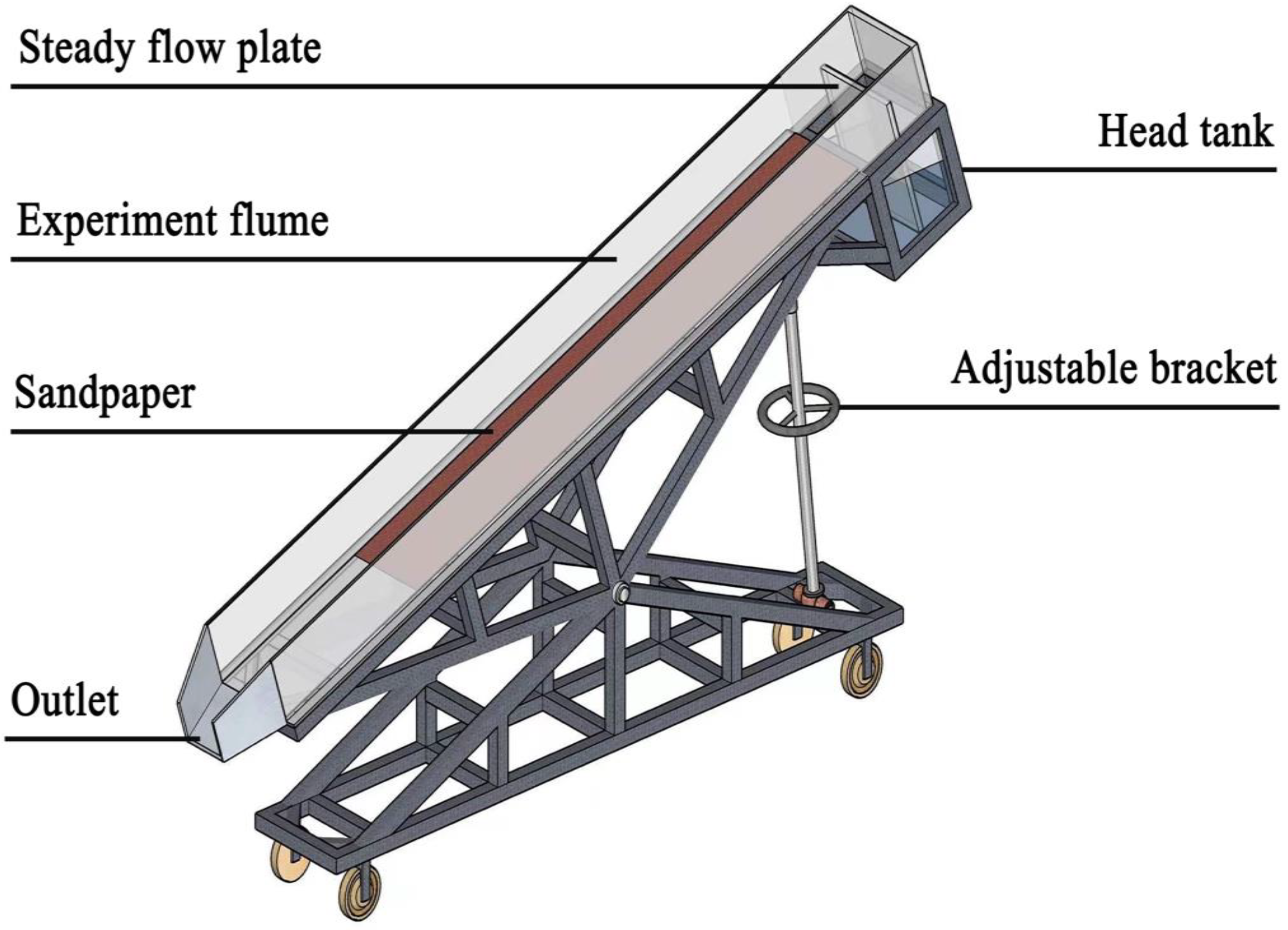
2.1. Experimental Design

The experimental plot consisted of an acrylic tank with an adjustable slope ranging from 0° to 30°, 3.8 m in length, 0.3 m in width, and 0.2 m in depth (Figure 1). A grid-shaped flow stabilizer was installed at the inlet of the tank to maintain the stability of the inflow water. The water supply used for the experiment came from a rectangular tank equipped with a low-flow water pump (QDX100-8-3.5, SRCH, Shanghai, China). The experimental flow was regulated using a glass rotor flow meter (LZB-40, SKJYLEAN, Suzhou, China) designed for a range of 250–2500 L/h. To achieve a uniform roughness scale on the bed, the bottom of the tank was lined with 40-mesh water sandpaper with a 0.38 mm roughness ($k_{sb}$). Rigid vegetation, which is a common type of vegetation used in experiments, is typically simulated using cylinders [31]. In this experiment, rigid vegetation was simulated using 2 cm diameter PVC pipes, with the vegetation-covered section of the tank extending 2 m with a 20 cm section reserved at the front as a flow stabilization area (Figure 2b). Experiments were conducted using 95, 187, and 286 rigid vegetation stems, as shown in Figure 2a. The rigid vegetation was arranged in a grid pattern, where the front and back rows formed a regular triangular structure. The coverage was defined as the ratio of the total stem cross-sectional area to the area of the covered region, calculated as follows:

$$C_r={\displaystyle \frac{N\mathsf{\pi }{D}^2}{4BL}}$$

(1)

$$C_r={\displaystyle \frac{N\mathsf{\pi }{D}^2}{4BLcos\theta }}$$

(2)

Equation (1) calculates vegetation coverage perpendicular to the slope direction (BS), where Cr is the vegetation coverage, N is the number of rigid vegetation cells in the test area, D is the diameter of the PVC pipe (0.02 m), B is the width of the experimental flume (0.3 m), and L is the length of the area covered by vegetation (2.0 m). For vegetation perpendicular to the horizontal plane (BH), coverage was calculated using the formula for the area of an ellipse (Equation (2)), where θ is the angle of the slope.

Slopes θ were set at 5°, 10°, 15°, and 20°, which resulted in slope ratios S of 0.0872, 0.1737, 0.2588, and 0.3420, respectively. The designed discharge rates were 5, 10, 20, 30, and 40 L·min⁻¹, which corresponded to per-width flow rates of 0.000278, 0.000556, 0.001111, 0.001667, and 0.002222 m³·m⁻¹·s⁻¹, respectively, with five levels of treatment. Three longitudinal observation sections were set along the flume from top to bottom, at 0–0.75 m, 0.75–1.5 m, and 1.25–2.0 m, respectively. Water depth h was measured using a water-level gauge (model: SCM60, The Leader, Shanghai, China; accuracy ± 0.01 mm). In each of the three sections, measurements were taken four times, totaling twelve measurements, which were averaged to obtain the final results. If the standard deviation of the results was >5%, re-testing was necessary.

2.2. Hydrodynamic Parameters

The formula for calculating mean velocity u is as follows:

$$u={\displaystyle \frac{Q}{h\times b_1}}$$

(3)

where Q is the design flow rate (m³·s⁻¹), h is the average water depth of the cross-section (m), and b₁ is the effective width of the water flow in the experiment (m).

Equation (4) defines b₁ as follows:

$$b_1=B\times (1-C_r)$$

(4)

Equation (5) was used for calculating the Reynolds number Re, as follows:

$$Re={\displaystyle \frac{uR}{{\nu }_0}}$$

(5)

where R is the hydraulic radius (m) and ${\nu }_0$ is the kinematic viscosity (m²·s⁻¹), which was calculated with Equation (5), as follows:

$${\nu }_0={\displaystyle \frac{0.01775}{1+0.0337\mathrm{t}+0.00022t^2}}$$

(6)

where t is the reading from the thermometer near the flow stabilizer (°C).

Equation (7) was used for calculating the Darcy–Weisbach resistance coefficient f, as follows:

$$f={\displaystyle \frac{8gRS}{u^2}}$$

(7)

Equation (8) was used to calculate the hydraulic radius R:

$$R={\displaystyle \frac{A}{P}}$$

(8)

where A is the cross-sectional area (m²) through which water passes, which is calculated as follows:

$$A=b_1\times h$$

(9)

P is the wetted perimeter (m) and is calculated as follows:

$$P={\displaystyle \frac{2HL+\left(BL-\frac{N\pi D^2}{4}\right)+\pi DhN}{L}}$$

(10)

$$P={\displaystyle \frac{2HL+\left(BL-\frac{N\pi D^2}{4cos\theta }\right)+\frac{\pi DhN}{cos\theta }}{L}}$$

(11)

Equation (10) is the calculation formula for the wetted perimeter of vegetation oriented perpendicularly to the slope (BS), and Equation (11) is for vegetation oriented perpendicularly to the horizontal plane (BH).

2.3. Data Processing

Model Accuracy Assessment Indicators

The accuracy of the mean velocity prediction model was assessed using the adjusted coefficient of determination, Adj.R², as well as the Nash–Sutcliffe efficiency coefficient, NSE; the standard error of the coefficients, SE; and the relative root-mean-square error, RRMSE. The formulae for these three evaluation indicators are as follows:

$$R^2={\displaystyle \frac{{\left[{\sum }_i^n(O_i-\overline{O}\left)\right(P_i-\overline{P})\right]}^2}{{\sum }_i^n{(O_i-\overline{O})}^2{\sum }_i^n{(P_i-\overline{P})}^2}}$$

(12)

$$Adj{R}^2=1-(1-R^2){\displaystyle \frac{n-1}{n-k-1}}$$

(13)

$$NSE=1-{\displaystyle \frac{{\sum }_{i=1}^n{(O_i-P_i)}^2}{{\sum }_{i=1}^n{(O_i-\overline{O})}^2}}$$

(14)

$$RRMSE={\displaystyle \frac{\sqrt{(1/n){\sum }_{i=1}^n{(O_i-P_i)}^2}}{\overline{O}}}$$

(15)

$$SE=\sqrt{{\displaystyle \frac{{\mathsf{\sigma }}^2}{{\sum }_{i=1}^n{(O_i-\overline{O})}^2}}}$$

(16)

where $O_i$ is the observed value, $\overline{O}$ is the mean of the observed values, $P_i$ is the simulated value, $\overline{P}$ is the mean of the simulated values, ${\mathsf{\sigma }}^2$ is the variance of the residuals, n is the number of samples, and k is the number of parameters.

2.4. Statistical Analyses

One-way analysis of variance (ANOVA) tests were conducted on the mean velocities under different flow rates, slopes, coverage levels, and types of coverage using SPSS 26 software (IBM SPSS Statistics, Armonk, NY, USA) with a significance level of p < 0.05. The nonlinear regression fitting function in SPSS 26 was used to construct a mean velocity prediction model. R Studio 4.2.0 (R Core Team, Vienna, Austria) and Origin 2023 (OriginLab Corporation, Northampton, MA, USA) were used to create graphics for visualization purposes.

3. Results

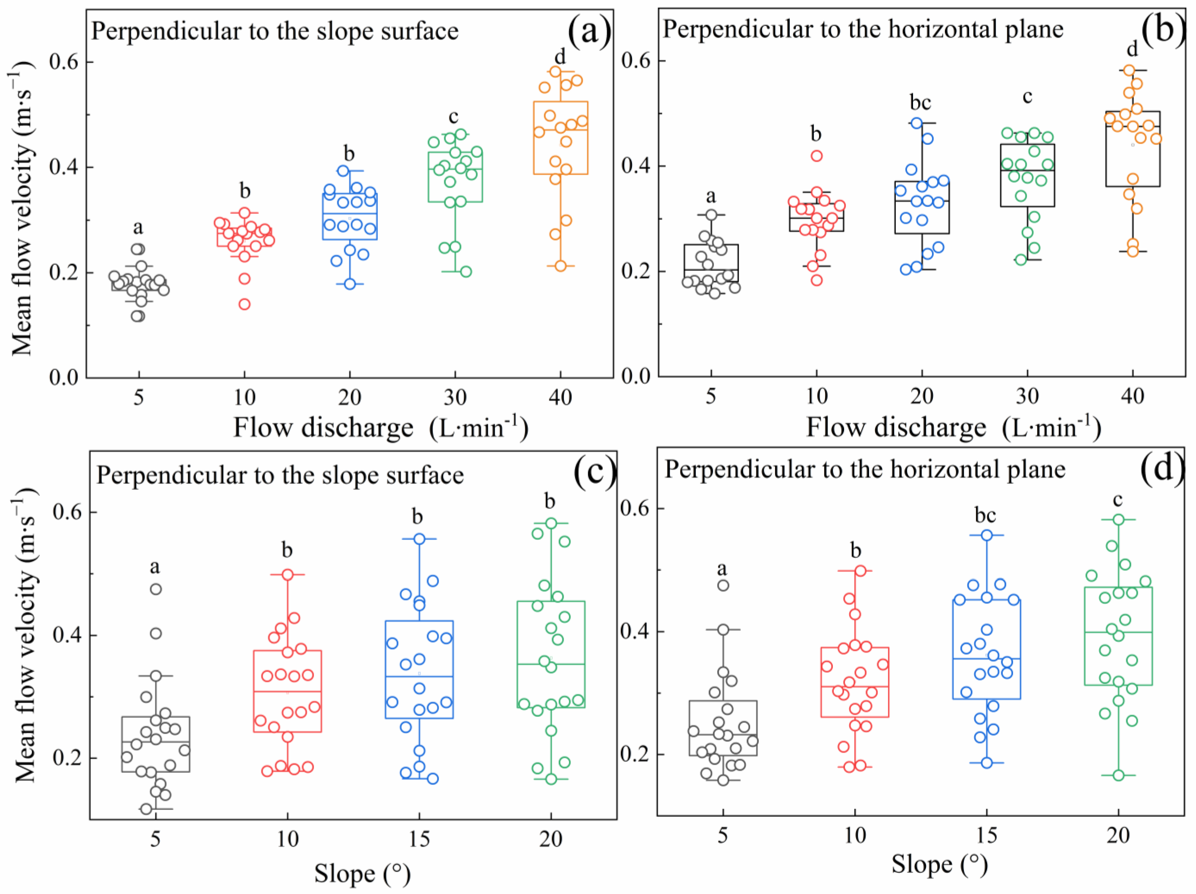
3.1. The Impact of Flow Rate and Slope on Mean Velocity

As the flow rate increased, the distribution range of the mean velocity increased, with flow rates of 5, 10, 20, 30, and 40 L·min⁻¹ showing mean velocity distribution ranges of 0.117 to 0.245 m·s⁻¹, 0.140 to 0.314 m·s⁻¹, 0.178 to 0.393 m·s⁻¹, 0.202 to 0.463 m·s⁻¹, and 0.213 to 0.582 m·s⁻¹ for BS; and 0.158 to 0.307 m·s⁻¹, 0.183 to 0.419 m·s⁻¹, 0.204 to 0.482 m·s⁻¹, 0.222 to 0.463 m·s⁻¹, and 0.238 to 0.582 m·s⁻¹ for BH, respectively (Figure 3). These results indicated that the flow rate and slope significantly affected the mean velocity distribution range (p < 0.05). A comparison of the two vegetation conditions revealed that at lower flow rates (5, 10, and 20 L·min⁻¹), the range of mean velocity under BS was smaller than that under BH. At higher flow rates (30 and 40 L·min⁻¹), the mean velocity distribution range under BS conditions was similar to that under BH conditions. As the slope increased, the distribution range of the mean velocity also increased. At slopes of 5°, 10°, 15°, and 20°, the ranges were 0.117 to 0.475 m·s⁻¹, 0.179 to 0.498 m·s⁻¹, 0.167 to 0.557 m·s⁻¹, and 0.166 to 0.582 m·s⁻¹ for BS conditions; and 0.158 to 0.475 m·s⁻¹, 0.179 to 0.498 m·s⁻¹, 0.186 to 0.557 m·s⁻¹, and 0.166 to 0.582 m·s⁻¹ for BH conditions, respectively, indicating that the range of the mean velocity distributions was similar under both BS and BH conditions.

3.2. The Impact of Rigid Vegetation on Mean Velocity

Under rigid vegetation cover conditions, the mean velocity of the slope flow was influenced by a combination of vegetation coverage, flow rate, and slope. At low flow rates, the mean velocity initially increased and then decreased with changes in vegetative coverage (Figure 4). For instance, at a slope of 5° and flow rate of 5 L·min⁻¹, the mean velocity increased to 0.158, 0.177, 0.145, and 0.117 m·s⁻¹ with increasing coverage (N = 0–286) under BS conditions, while at a slope of 10° and flow rate of 10 L·min⁻¹, the mean velocity rates were 0.274, 0.312, 0.301, and 0.279 m·s⁻¹ with increasing coverage (N = 0–286) under BH conditions. At a slope of 5° and a flow rate of 30 L·min⁻¹, the mean velocities with increasing BH coverage conditions were 0.403, 0.274, 0.245, and 0.222 m·s⁻¹, indicating that at lower slopes, as the flow rate increased, the mean velocity gradually decreased. At medium-to-high slopes (10–20°), the mean velocity gradually decreased and then increased as the flow rate increased, and was most pronounced at a flow rate of 20 L·min⁻¹. Indeed, at a slope of 20° and a flow rate of 20 L·min⁻¹, the mean velocities with increasing coverage were 0.393, 0.348, 0.288, and 0.358 m·s⁻¹ under BS conditions. At a flow rate of 5 L·min⁻¹ with slopes of 15° and 20°, the rates of change in the range of mean velocities were 54.9% and 85.3%, respectively, indicating that as the flow rate increased, the differences in velocity between different coverage levels decreased and the rate of velocity stabilized. However, at a flow rate of 40 L·min⁻¹ with slopes of 15° and 20°, the rates of change in the range of mean velocities were only 23.9% and 20.9%, respectively, suggesting that the trend in the mean velocity change at high discharge was gentler than that at low discharge. In addition, the influence of rigid vegetation on velocity at low discharge was more apparent.

The ANOVA tests showed that under different slope and flow conditions, the coverage of rigid vegetation and the vegetation type had a significant effect on the mean flow velocity (p < 0.05). Post hoc tests were used to compare the flow velocities between two types of rigid vegetation (BS and BH) under the same hydraulic conditions, and specific results indicated by “a”, “b”, “c”, “d”, “e”, and “f” labels are shown in Figure 4. For example, under the conditions of a 5° slope and a flow rate of 10 L·min⁻¹, the mean flow velocity for BH was significantly higher than that for BS at all three coverage levels (p < 0.05). However, under the conditions of a 20° slope and a flow rate of 5 L·min⁻¹, although the mean flow velocity for BH was also higher than that for BS at all three coverage levels, the difference was not statistically significant where N = 187 (p > 0.05). To compare the effects of the two types of rigid vegetation on the mean velocity, we used a velocity ratio defined as the velocity under BS conditions (u_BS) divided by that under BH conditions (u_BH). A velocity ratio greater than 1 indicated that the velocity under the BS conditions was greater than that under the BH conditions, and vice versa. Correlation tests revealed significant relationships among the velocity ratio and the Reynolds number ratio, resistance coefficient ratio, and flow rate (p < 0.05), with Pearson correlation coefficients of 0.83, –0.95, and 0.61, respectively. As the Reynolds number ratio and flow rate increased, the velocity ratio increased (Figure 5), whereas an increase in the resistance ratio led to a decreased velocity ratio. Figure 5a and 5b, respectively, show the relationships between the velocity ratio and the Reynolds number ratio and between the velocity ratio and the flow rate. The R² values of the linear equations are 0.70 and 0.37, respectively. Overall, these results indicate that not only does the difference in rigid vegetation coverage affect the average flow velocity, but it is also affected by the direction of rigid vegetation growth (BS and BH).

3.3. Mean Velocity Prediction Model

The prediction of mean velocity has been a major area of research among scholars [35,36], with the mean velocity being expressed as a power function of slope and flow rate, with vegetation coverage being a determinant of exponential size [37]. In this study, a nonlinear regression analysis was performed on the experimental data, and the results of this analysis are presented in Table 1.

Table 1. Mean flow velocity prediction model for different flow rate and slope conditions.

Treatment	Fitting Formula		Adj.R2	NSE	RRMSE	SE
BS	$u=16.050Q^{0.424}{S}^{0.320}$	(17)	0.83	0.83	0.15	0.049
BH	$u=7.481Q^{0.319}{S}^{0.331}$	(18)	0.77	0.77	0.15	0.060
ALL	$u=9.328Q^{0.347}{S}^{0.356}$	(19)	0.80	0.80	0.15	0.042

Notes: BS, perpendicular to the slope surface; BH, perpendicular to the horizontal plane; ALL, all data combined; Adj.R², adjusted R square; NSE, Nash–Sutcliffe efficiency; RRMSE, relative root-mean-square error; SE, standard error of the coefficients; u, mean velocity; S, slope ratio; Q, flow rate (m³·s⁻¹).

Table 1. Mean flow velocity prediction model for different flow rate and slope conditions.

Treatment	Fitting Formula		Adj.R2	NSE	RRMSE	SE
BS	$u=16.050Q^{0.424}{S}^{0.320}$	(17)	0.83	0.83	0.15	0.049
BH	$u=7.481Q^{0.319}{S}^{0.331}$	(18)	0.77	0.77	0.15	0.060
ALL	$u=9.328Q^{0.347}{S}^{0.356}$	(19)	0.80	0.80	0.15	0.042

Notes: BS, perpendicular to the slope surface; BH, perpendicular to the horizontal plane; ALL, all data combined; Adj.R², adjusted R square; NSE, Nash–Sutcliffe efficiency; RRMSE, relative root-mean-square error; SE, standard error of the coefficients; u, mean velocity; S, slope ratio; Q, flow rate (m³·s⁻¹).

The relationship between the predicted and measured mean flow velocities were calculated using Equation (19), which indicated that the Adj.R² under BH conditions was 0.77 (Equation (18)), while the Adj.R² for the prediction model fitted with all data was 0.80 (Equation (19); Figure 6c). Because of the more complex dynamics of overland flow compared to open-channel flow, especially when surface runoff is influenced by vegetation, using only flow and slope for prediction is not ideal [38]. For slopes covered with vegetation, proposed theories such as vegetation equivalent resistance coefficients [30] and vegetation-based roughness height [39] integrate the effects of vegetation on overland flow with the underlying surface impacts to enhance the practicality of hydraulic models. Rigid vegetation acts as a roughness element on slopes and its impact can be quantified using the resistance coefficient formula for rough areas, as follows [39]:

$$f={\left(2\mathrm{l}\mathrm{o}\mathrm{g}{\displaystyle \frac{3.7h}{k_{sv}}}\right)}^{-2}$$

(20)

Equations (7) and (20) calculate the resistance coefficients; thus, by combining and rearranging them, we can derive the vegetation equivalent roughness height $k_{sv}$ (mm):

$$k_{sv}={\displaystyle \frac{3.7h}{{10}^{0.5\sqrt{\frac{u^2}{8gRS}}}}}$$

(21)

Because the substrate used in this experiment was 40-mesh sandpaper, the roughness height of the slope outside the vegetated area remained constant ($k_{sb}$ = 0.38 mm). Adding the rigid vegetation equivalent roughness height $k_{sv}$ to that of the non-vegetated area $k_{sb}$ yielded the equivalent roughness height $k_{se}$ (mm) of the slope under stiff vegetation cover. The resulting formula is as follows:

$$k_{se}=k_{sv}+\left(1-Cr\right)k_{sb}$$

(22)

The equivalent roughness height, $k_{se}$, of the slope under stiff vegetation was correlated with the slope, flow, and coverage. For easier field observation and application, a nonlinear fit using the equivalent roughness height, $k_{se}$; the flow rate, Q; the energy slope, S; and the coverage, Cr, was performed using the following equation:

$$k_{se}=132.154Q^{0.718}{S}^{-0.753}{e}^{6.984Cr}$$

(23)

The Adj.R² value of Equation (23) was 0.78, indicating that the model structure was reasonable. Manning’s resistance coefficient, n, depends on the vegetation coverage and soil type [40]. Because this experiment was a fixed-bed test, the Manning’s coefficient was primarily influenced by the coverage of rigid vegetation. The formula used for calculating Manning’s coefficient, $n_v$, under vegetation cover is as follows:

$$n_v={\displaystyle \frac{1}{u}}{R}^{m_1}{S}^{m_2}$$

(24)

where $m_1$ and $m_2$ are the exponents of the hydraulic radius R and energy slope S, respectively. Compared with the basic Manning formula, the use of the hydraulic radius R was more appropriate because of the changes in water depth, h, caused by rigid vegetation cover. Wu et al. [41] found that Manning’s coefficient decreases with increasing water depth and increases with increasing slope roughness. This is similar to the findings of Yang et al. [42], who reported that the Manning’s coefficient, $n_b$, for slopes without vegetation cover can be expressed as a function of the slope roughness height, $k_{sb}$, and water depth, h, using the following specific function form:

$$n_b={\displaystyle \frac{{k_{sb}}^{m_3}}{h^{m_4}}}$$

(25)

where $m_3$ and $m_4$ are the exponents of the slope roughness height $k_{sb}$ and water depth h, respectively. Similarly, by replacing the slope roughness height $k_{sb}$ in Equation (25) with the equivalent roughness height $k_{se}$ under a rigid vegetation cover, the following formula for the equivalent vegetation Manning coefficient $n_{ve}$ was derived, as follows:

$$n_{ve}={\displaystyle \frac{{k_{se}}^{m_3}}{h^{m_4}}}$$

(26)

By combining Equations (24)–(26), the model expression for the mean flow velocity u was constructed:

$$u={\displaystyle \frac{{a_{1}R}^{a_2}{S}^{a_3}{h}^{a_4}}{{k_{se}}^{a_5}}}$$

(27)

where $a_1$, $a_2$, $a_3$, $a_4$, and $a_5$ are the constants. The equivalent roughness height, $k_{se}$, of the slope in Equation (27) can be calculated using Equation (23), and the flow velocity prediction model was thus obtained after nonlinear fitting of the experimental data (

Table 2. The mean velocity prediction model using the equivalent roughness height, $k_{se}$.

Treatment	Fitting Formula		Adj.R2	NSE	RRMSE	SE
BS	$u={\displaystyle \frac{1.975R^{6.023}{S}^{0.741}{h}^{-5.892}}{{k_{se}}^{-0.813}}}$	(28)	0.88	0.88	0.12	0.044
BH	$u={\displaystyle \frac{1.705R^{5.050}{S}^{0.683}{h}^{-4.940}}{{k_{se}}^{-0.677}}}$	(29)	0.88	0.88	0.12	0.041
ALL	$u={\displaystyle \frac{1.369R^{5.300}{S}^{0.731}{h}^{-5.222}}{{k_{se}}^{-0.774}}}$	(30)	0.87	0.86	0.12	0.036

Notes: BS, perpendicular to the slope surface; BH, perpendicular to the horizontal plane; ALL, all data combined; Adj.R², adjusted R square; NSE, Nash–Sutcliffe efficiency; RRMSE, relative root-mean-square error; SE, standard error of the coefficients; u, mean velocity; S, slope ratio; R, hydraulic radius (m); h, average water depth (m); $k_{se}$, equivalent roughness height (mm).

).

4. Discussion

4.1. The Impact of Flow Rate and Slope on Mean Velocity

The mean flow velocity, u, a crucial hydraulic characteristic in soil erosion modeling, is influenced by the flow rate [43], slope, and surface conditions. In this study, slope and flow rate increased the mean flow velocity, which suggested that the gravitational potential energy of the water flow rises as the slope becomes steeper, resulting in higher flow velocities on the slope. This outcome aligns with the findings of Zhang et al. [44] and Liu et al. [32]. Whether on a smooth bare slope or a slope with surface cover, u remains highly correlated with slope and flow rate [6]. For instance, Liu et al. [45] found that on gravel-covered slopes, the correlation coefficients between the mean flow velocity, flow rate, and slope were 0.716 and 0.674, respectively. Similarly, the slope factor and rate of straw addition could be used to estimate u on slopes with added straw (R² = 0.91) [46]. However, Ali et al. [47] found that under mobile bed conditions, the slope did not significantly affect u, which may be due to the different substrate conditions. In our study, the substrate and bed conditions were kept constant throughout the experiment to explore how the flow rate and slope affected the morphology and roughness of erosive slopes. Giménez et al. [48] suggested that slope roughness is positively correlated with slope; thus, the greater the slope, the rougher the slope surface. A rougher substrate can offset the kinetic energy converted from the gravitational potential energy [49], thus resulting in no significant change in u.

4.2. The Impact of Rigid Vegetation on Mean Velocity

It is commonly believed that vegetation increases surface roughness, and that the energy of the slope flow is mainly consumed by the surface roughness caused by the aboveground parts of vegetation [50]. Thus, vegetation reduces the mean flow velocity, u, on slopes. For example, under three different vegetation covers, the flow velocity on slopes decreased by 28–30% [15]. Liu et al. [51] added different amounts of straw to slopes to increase surface roughness and found that the flow velocity decreased by 28.44%, 44.09%, and 55.56%. However, in our experiment, there was no monotonic decrease in the association between u and the coverage of rigid vegetation, and u was differentially influenced by the test conditions (Figure 4). At low flow rates and with increases in slope, u fluctuates as follows: it first increases, then decreases, and then finally increases. In comparison, at high flow rates, u fluctuates as follows: it first decreases and then increases in response to an increase in the vegetation cover. The primary reason for the increase in u was that the rigid vegetation changed the cross-sectional area of the flow on the slope, which impacted the spatial distribution of the water [15]. Rigid vegetation was the primary roughness element on the slope and reduced the flow velocity due to its obstructive effect, while also accelerating water flow through non-vegetated areas, forming concentrated flows and increased velocity [52]. Our findings are supported by those of Wu et al. [23], who observed that the flow velocity behind rigid vegetation was lower than that within vegetation gaps using a three-dimensional laser Doppler velocimeter. Vegetation also affects water depth by increasing the water level upstream and decreasing it downstream of vegetation [53]. This backwater-induced local pressure difference increases the local flow velocity and shear stress, increasing the erosion risk near vegetated areas [54]. Zhao et al. [28] used PVC pipes to replicate rigid vegetation and showed that the flow velocity increases marginally with greater coverage. At low flow rates, the critical coverage for the increase in the mean flow velocity was low, and this critical coverage increased as the flow rate increased. The main resistance to flow on slopes comes from the particle resistance generated by the slope and the form resistance created by vegetation [55], with particle resistance generally decreasing as the flow rate and slope increase [38]. At low flow rates, the slope flow is slower and shallower, and vegetation with low coverage compresses the water flow space, increasing the flow velocity. As the flow rate increases, both the flow velocity and water depth increase, at which time the particle resistance on the slope is gradually replaced by the form resistance of the vegetation. The increased flow velocity owing to the compression of the water cross-sectional area by vegetation at low coverage cannot replace the reduced flow velocity owing to vegetation form resistance [34]. Under these conditions, the compression of the water flow space by high-coverage vegetation becomes more pronounced [56], leading to increased flow velocity. The trend in changes in mean flow velocity depends on whether particle resistance or form resistance predominates in the slope flow [57].

For the two different types of rigid vegetation used in our study (BS and BH), the morphological differences resulted in different degrees of obstruction to the water flow, which affected the mean flow velocity. We found that under BS conditions, the average flow velocity (0.331 m·s⁻¹) was higher than that under BH conditions (0.311 m·s⁻¹). The velocity ratio was positively correlated with both the flow ratio and the Reynolds number ratio, while in contrast, it was found to be negatively correlated with the resistance coefficient ratio. We found that most Reynolds number ratios and velocity ratios were generally less than 1 (Figure 5), indicating that under BS conditions, the rigid vegetation significantly obstructed water flow, inhibited changes in the slope flow state, and lowered the flow velocity. Similarly, an increase in flow suggested greater water depth. Under the BS conditions, vegetation compressed the flow more significantly; therefore, under high-flow and BS conditions, the flow velocity gradually exceeded that reported under the BH conditions. These findings are congruent with those of Schoelynck et al. [58], who postulated that vegetation on a slope provides less hindrance to water flow because it is more streamlined. Shan et al. [59] also found that the angle at which vegetation is deflected increases water flow when the water flow contacts the vegetation perpendicularly (e.g., BS)—i.e., it encounters greater obstruction—whereas when the vegetation is angled (e.g., BH), it exerts less drag, making it easier for the flow to bypass [60]. In this study, the increase in rigid vegetation coverage altered the connectivity of the water flow. For slope flow under BS conditions, as the number of rigid vegetation N increased from 95 to 286, the coefficient of variation in the mean flow velocity was 30.72%, 35.27%, 29.82%, and 41.61%, respectively. In contrast, for slope flow under BH conditions, the coefficient of variation in the mean flow velocity was 25.68%, 29.82%, and 33.92% as N increased from 95 to 286. In the arrangement of a regular grid, the increase in vegetation coverage made the water flow paths more complex, and the variation in mean flow velocity under different hydraulic conditions became more complicated. Therefore, the coefficient of variation in the flow velocity increased with the increase in coverage. Additionally, the coefficient of variation under BS conditions was consistently higher than that under BH conditions, possibly due to the greater impact of rigid vegetation on water flow in BS conditions.

4.3. Evaluation of Mean Flow Velocity Prediction Models

Traditional hydraulic models consider flow velocity as a power function of both the flow rate and slope [32]; however, on vegetated slopes, flow rate and slope are no longer the sole factors affecting flow velocity [61]. Equations (17)–(19) reflect the mean flow velocity prediction models fitted using the slope and flow rate as variables. For all data, Figure 6c shows that the data points predicted by Equation (19) are close to the 1:1 line, although some data points are more scattered. In comparison, the data points predicted by Equation (30) are uniformly distributed near the 1:1 line (Figure 6d), with less dispersion than those predicted by Equation (19). This demonstrates that utilizing the vegetation equivalent roughness height to predict u is rational and yields a highly accurate model. Furthermore, it is unreasonable to predict u solely based on the flow rate and slope on slopes with rigid vegetation; therefore, factors related to vegetation must be considered when predicting mean flow velocities.

To enhance the representativeness of our model results, we examined the flow velocity models from the literature [17,31]. Nearing et al. [31] reported experiments that were conducted on soil slopes and their results showed that the model’s Adj.R², NSE, RRMSE, and SE were 0.45, −0.01, 0.34, and 0.082, respectively. Our results had a high dispersion of data points near the 1:1 line, which indicated that this model is unsuitable for slopes covered with rigid vegetation (Figure 6a). The model did not consider the slope factor because the roughness of soil slopes increased with slope during erosion, which offset the contribution of the slope to u [48]. This is similar to Emmett’s [21] study, which concluded through field experiments that slope roughness slows flow velocity and increases water depth, with the increase in water depth being primarily attributed to vegetation and topographic features. Cen et al. [17] reported a model with Adj.R², NSE, RRMSE, and SE values of 0.61, 0.55, 0.22, and 0.082, respectively. This model considered factors such as hydraulic radius, slope, vegetation coverage, and water depth and was more accurate than the previous model [31]. However, the equation specifically developed for modeling vegetated slope flow velocities did not assess flow velocities on bare slopes [17]. We found that this model was relatively dispersed near the 1:1 line primarily because of differences in the type of simulated vegetation (Figure 6b). Additionally, this model was developed specifically for tufted synthetic grass, which has a stronger disturbance effect on water flow. As a result, the model predicts a higher degree of variability in the average flow velocity compared to Equations (19) and (30). The influence of vegetation on the hydrodynamic properties of surface water is affected not only by the above- and underground parts of the vegetation [16] but also by different morphological features of the vegetation [62]. As shown in

Table 3. Comparison of different mean velocity prediction models.

Mean Flow Velocity Prediction Model	Adj.R2	NSE	RRMSE	SE
Nearing et al. [31]	0.45	−0.01	0.34	0.082
Cen et al. [17]	0.61	0.55	0.22	0.053
This study’s Equation (19)	0.80	0.80	0.15	0.042
This study’s Equation (30)	0.87	0.86	0.12	0.036

Notes: Adj.R², adjusted R square; NSE, Nash–Sutcliffe efficiency; RRMSE, relative root-mean-square error; SE, standard error of the coefficients.

, Equation (30) demonstrates significant improvements in all metrics, especially in Adj.R², which shows an enhancement ranging from 8.75% to 93.3% compared to other models. This indicates that this model exhibits superior fitting and predictive efficiency. Additionally, the lower RRMSE (0.12) and SE (0.036) values suggest that this model has smaller prediction errors, providing better accuracy and stability.

5. Conclusions

We conducted indoor simulation experiments to investigate the mechanisms by which rigid vegetation coverage and growth direction affect the mean flow velocity under conditions of four slope gradients, five flow rates, four levels of vegetation coverage, and two vegetation growth directions. First, we analyzed the impact of slope and flow rate on mean flow velocity and found that both significantly affected mean flow velocity (p < 0.05), with the mean flow velocity increasing as both the slope and flow rate increased. Second, we analyzed the impact of rigid vegetation on the mean flow velocity, observing both similarities and differences with previous studies. Our results indicate that rigid vegetation coverage not only reduces the mean flow velocity but can also increase it under certain conditions, primarily owing to the compression of the water flow path by the rigid vegetation. Additionally, the mean flow velocity under BH conditions was generally higher than that under BS conditions, and the velocity ratio was significantly correlated with the Reynolds number ratio, resistance coefficient ratio, and flow rate (p < 0.05). Finally, we established a model to predict the mean flow velocity by combining vegetation equivalent roughness and the Manning formula. The results showed that this model could accurately predict the average flow velocity (Adj.R² = 0.87, NSE = 0.86, RRMSE = 0.12, and SE = 0.036).

On natural slopes, the conditions of the underlying surface change due to water flow erosion, and the movement of surface soil particles alters surface roughness. This study was conducted in a fixed-bed flume, which did not account for the effects of bed erosion on flow velocity on slopes. Furthermore, in the field, vegetation growth can exhibit more complex characteristics, such as combinations of different stem diameters, different vegetation cover patterns, and combinations of flexible and rigid vegetation. These vegetation characteristics can all impact the hydrodynamic properties of slope flows. Additionally, the response of flow velocity to slope erosion is also crucial. Therefore, future research should focus on establishing the relationship between slope flow velocity and soil erosion with different vegetation characteristics, which will further contribute to the improvement of soil erosion prediction models.

References

1. Zhou, Y.; Yi, Y.; Liu, H.; Tang, C.; Zhang, S.H. Spatiotemporal dynamic of soil erosion and the key factors impact processes over semi-arid catchments in Southwest China. Ecol. Eng. 2024, 201, 14. [Google Scholar] [CrossRef]
2. Zeng, X.; Peng, X.D.; Liu, T.T.; Dai, Q.H.; Chen, X.Y. Runoff generation and erosion processes at the rock-soil interface of outcrops with a concave surface in a rocky desertification area. Catena 2024, 239, 11. [Google Scholar] [CrossRef]
3. Xu, E.Q.; Zhang, H.Q. Change pathway and intersection of rainfall, soil, and land use influencing water-related soil erosion. Ecol. Indic. 2020, 113, 14. [Google Scholar] [CrossRef]
4. Zhang, X.C.; Zheng, F.L.; Chen, J.; Garbrecht, J.D. Characterizing detachment and transport processes of interrill soil erosion. Geoderma 2020, 376, 15. [Google Scholar] [CrossRef]
5. Ma, Q.H.; Zhang, K.L.; Cao, Z.H.; Wei, M.Y.; Yang, Z.C. Soil detachment by overland flow on steep cropland in the subtropical region of China. Hydrol. Process. 2020, 34, 1810–1820. [Google Scholar] [CrossRef]
6. Wang, G.Y.; Sun, G.R.; Li, J.K.; Li, J. The experimental study of hydrodynamic characteristics of the overland flow on a slope with three-dimensional Geomat. J. Hydrodyn. 2018, 30, 153–159. [Google Scholar] [CrossRef]
7. Wang, H.M.; Ni, W.K.; Yuan, K.Z.; Ren, S.Y. An experimental study on the behavior of loess-clay mixtures upon wetting and its implications for tillage on the Loess Plateau. Soil Tillage Res. 2024, 240, 12. [Google Scholar] [CrossRef]
8. Zhang, S.-Q.; Wang, Y.-W.; Zhang, H.-B.; Lyu, F.-G.; Yang, T.-Z.; Li, Y.-B.; Yao, C.-C. Investigating the Loess Plateau’s coevolution of precipitation and natural vegetation cover. Environ. Earth Sci. 2024, 83, 15. [Google Scholar] [CrossRef]
9. Chen, Y.; Wang, K.; Lin, Y.; Shi, W.; Song, Y.; He, X. Balancing green and grain trade. Nat. Geosci. 2015, 8, 739–741. [Google Scholar] [CrossRef]
10. Zeng, Y.X.; Liu, Y.; Yu, X.B. Contribution of hydrological connectivity to the retention of soil organic carbon by vegetation patches: Insight from a dryland hillslope on the Loess Plateau, China. Catena 2022, 216, 9. [Google Scholar] [CrossRef]
11. Zhang, Z.; Zou, J.; Yu, W.; Li, Q.; Feng, Z.; Zhang, H. Resilience and community dynamics of understorey vegetation in Mongolian pine plantations at the southeastern edge of the Mu Us Sandy Land, China. For. Ecol. Manage. 2024, 555, 9. [Google Scholar] [CrossRef]
12. Montakhab, A.; Yusuf, B.; Ghazali, A.H.; Mohamed, T.A. Flow and sediment transport in vegetated waterways: A review. Rev. Environ. Sci. Bio-Technol. 2012, 11, 275–287. [Google Scholar] [CrossRef]
13. Wu, S.F.; Wu, P.T.; Feng, H.; Merkley, G.P. Effects of alfalfa coverage on runoff, erosion and hydraulic characteristics of overland flow on loess slope plots. Front. Environ. Sci. Eng. China 2011, 5, 76–83. [Google Scholar] [CrossRef]
14. Liu, C.; Zhang, K.; Wei, S.; Wang, P.; Cen, Y.; Xia, J. Evaluation of the effects of grass and shrub cover on overland flow resistance and its attributes under simulated rainfall. J. Hydrol. 2023, 626, 14. [Google Scholar] [CrossRef]
15. Li, C.J.; Pan, C.Z. Overland runoff erosion dynamics on steep slopes with forages under field simulated rainfall and inflow. Hydrol. Process. 2020, 34, 1794–1809. [Google Scholar] [CrossRef]
16. Zhang, G.H.; Hu, J.J. Effects of patchy distributed Artemisia capillaris on overland flow hydrodynamic characteristics. Int. Soil Water Conserv. Res. 2019, 7, 81–88. [Google Scholar] [CrossRef]
17. Cen, Y.; Zhang, K.; Peng, Y.; Rubinato, M.; Zhang, H.; Shang, H.; Li, P. Quantification of the effects on the flow velocity caused by gramineous plants in the loess plateau in North-Western China. Geoderma 2023, 429, 15. [Google Scholar] [CrossRef]
18. Zhu, P.Z.; Zhang, G.H.; Wang, H.X.; Zhang, B.J.; Wang, X. Land surface roughness affected by vegetation restoration age and types on the Loess Plateau of China. Geoderma 2020, 366, 11. [Google Scholar] [CrossRef]
19. Vermang, J.; Norton, L.; Huang, C.; Cornelis, W.; da Silva, A.; Gabriels, D. Characterization of Soil Surface Roughness Effects on Runoff and Soil Erosion Rates under Simulated Rainfall. Soil Sci. Soc. Am. J. 2015, 79, 903–916. [Google Scholar] [CrossRef]
20. De Serio, F.; Ben Meftah, M.; Mossa, M.; Termini, D. Experimental investigation on dispersion mechanisms in rigid and flexible vegetated bed. Adv. Water Resour. 2018, 120, 98–113. [Google Scholar] [CrossRef]
21. Emmett, W.W. The Hydraulics of Overland Flow on Hillslopes; U.S. Geological Survey Professional Paper 662-A; U.S. Geological Survey: Washington, DC, USA, 1970. [Google Scholar]
22. Cen, Y.; Zhang, K.; Peng, Y.; Rubinato, M.; Liu, J.; Ling, P. Experimental study on the effect of simulated grass and stem coverage on resistance coefficient of overland flow. Hydrol. Process. 2022, 36, 17. [Google Scholar] [CrossRef]
23. Wu, Y.J.; Jing, H.F.; Li, C.G.; Song, Y.T. Flow characteristics in open channels with aquatic rigid vegetation. J. Hydrodyn. 2020, 32, 1100–1108. [Google Scholar] [CrossRef]
24. Teng, S.F.; Feng, M.Q.; Chen, K.L.; Wang, W.J.; Zheng, B.M. Effect of a Lateral Jet on the Turbulent Flow Characteristics of an Open Channel Flow with Rigid Vegetation. Water 2018, 10, 15. [Google Scholar] [CrossRef]
25. Fukaki, H.; Fujii, N.; Itoh, E.; Yoshioka, Y.; Nakamura, M.; Morita, M.T. Polar recruitment of RLD by LAZY1-like protein during gravity signaling in root branch angle control. Nat. Commun. 2020, 11, 76. [Google Scholar]
26. Waite, J.M.; Dardick, C. IGT/LAZY genes are differentially influenced by light and required for light-induced change to organ angle. BMC Biol. 2024, 22, 8. [Google Scholar] [CrossRef] [PubMed]
27. Nishimura, T.; Mori, S.; Shikata, H.; Nakamura, M.; Hashiguchi, Y.; Abe, Y.; Morita, M.T. Cell polarity linked to gravity sensing is generated by LZY translocation from statoliths to the plasma membrane. Science 2023, 381, eadh9978. [Google Scholar] [CrossRef] [PubMed]
28. Zhao, C.H.; Gao, J.E.; Zhang, M.J.; Wang, F.; Zhang, T. Sediment deposition and overland flow hydraulics in simulated vegetative filter strips under varying vegetation covers. Hydrol. Process. 2016, 30, 163–175. [Google Scholar] [CrossRef]
29. Zhao, C.H.; Gao, J.E.; Huang, Y.F.; Wang, G.Q.; Zhang, M.J. Effects of Vegetation Stems on Hydraulics of Overland Flow Under Varying Water Discharges. Land Degrad. Dev. 2016, 27, 748–757. [Google Scholar] [CrossRef]
30. Wang, W.-J.; Peng, W.-Q.; Huai, W.-X.; Katul, G.G.; Liu, X.-B.; Qu, X.-D.; Dong, F. Friction factor for turbulent open channel flow covered by vegetation. Sci. Rep. 2019, 9, 16. [Google Scholar] [CrossRef]
31. Nearing, M.A.; Simanton, J.R.; Norton, L.D.; Bulygin, S.J.; Stone, J. Soil erosion by surface water flow on a stony, semiarid hillslope. Earth Surf. Process. Landf. 1999, 24, 677–686. [Google Scholar] [CrossRef]
32. Liu, J.; Zhang, K.; Peng, Y.; Rubinato, M.; Zhang, H.; Li, P. Effect of gravel coverage on the hydrodynamic characteristics of overland flow on the Loess Plateau in China. J. Hydrol. 2013, 627, 22. [Google Scholar] [CrossRef]
33. Plew, D.R. Depth-Averaged Drag Coefficient for Modeling Flow through Suspended Canopies. J. Hydraul. Eng.-ASCE 2011, 137, 234–247. [Google Scholar] [CrossRef]
34. Fu, S.H.; Mu, H.L.; Liu, B.Y.; Yu, X.J.; Liu, Y.N. Effect of plant basal cover on velocity of shallow overland flow. J. Hydrol. 2019, 577, 8. [Google Scholar] [CrossRef]
35. Li, D.; Peng, Z.Y.; Liu, G.Q.; Wei, C.Y. Flow Structures in Open Channels with Emergent Rigid Vegetation: A Review. Water 2023, 15, 15. [Google Scholar] [CrossRef]
36. Di Stefano, C.; Ferro, V.; Pampalone, V.; Sanzone, F. Field investigation of rill and ephemeral gully erosion in the Sparacia experimental area, South Italy. Catena 2013, 101, 226–234. [Google Scholar] [CrossRef]
37. Zhang, K.D.; Wang, Z.G.; Wang, G.Q.; Sun, X.M.; Cui, N.B. Overland-Flow Resistance Characteristics of Nonsubmerged Vegetation. J. Irrig. Drainage Eng-ASCE 2017, 143, 9. [Google Scholar] [CrossRef]
38. Zhang, J.Z.; Zhang, S.T.; Wang, C.T.; Wang, W.J.; Ma, L.J. Influence of combined stem vegetation distribution and discretization on the hydraulic characteristics of overland flow. J. Clean Prod. 2022, 376, 20. [Google Scholar] [CrossRef]
39. Shang, H.; Zhang, K.; Wang, Z.; Yang, J.; He, M.; Pan, X.; Fang, C. Effect of varying wheatgrass density on resistance to overland flow. J. Hydrol. 2020, 591, 15. [Google Scholar] [CrossRef]
40. Jain, M.K.; Singh, V.P. DEM-based modelling of surface runoff using diffusion wave equation. J. Hydrol. 2004, 302, 107–126. [Google Scholar] [CrossRef]
41. Wu, F.C.; Shen, H.W.; Chou, Y.J. Variation of roughness coefficients for unsubmerged and submerged vegetation. J. Hydraul Eng.-ASCE 1999, 125, 934–942. [Google Scholar] [CrossRef]
42. Yang, P.; Li, R.; Pan, L.; Wang, Y.; Huang, K.; Zhang, L. Effects of surface roughness and vegetation coverage on Manning’s resistance coefficient to overland flow. Trans. CSAE 2020, 36, 106–114. [Google Scholar]
43. Zhang, G.H.; Liu, G.B.; Wang, G.L.; Wang, Y.X. Effects of patterned Artemisia capillaris on overland flow velocity under simulated rainfall. Hydrol. Process. 2012, 26, 3779–3787. [Google Scholar] [CrossRef]
44. Zhang, K.; Weber, P.L.; Jonge, L.W.D.; Wang, X.; Bai, Y.K. Effect of different underlying surfaces on hydraulic parameters of overland flow. Soil Tillage Res. 2023, 232, 10. [Google Scholar] [CrossRef]
45. Liu, X.N.; Fan, D.X.; Yu, X.X.; Liu, Z.Q.; Sun, J.M. Effects of simulated gravel on hydraulic characteristics of overland flow under varying flow discharges, slope gradients and gravel coverage degrees. Sci. Rep. 2019, 9, 13. [Google Scholar] [CrossRef] [PubMed]
46. Pan, C.Z.; Ma, L.; Shangguan, Z.P. Effectiveness of grass strips in trapping suspended sediments from runoff. Earth Surf. Process. Landf. 2010, 35, 1006–1013. [Google Scholar] [CrossRef]
47. Ali, M.; Sterk, G.; Seeger, M.; Stroosnijder, L. Effect of flow discharge and median grain size on mean flow velocity under overland flow. J. Hydrol. 2012, 452, 150–160. [Google Scholar] [CrossRef]
48. Giménez, R.; Planchon, O.; Silvera, N.; Govers, G. Longitudinal velocity patterns and bed morphology interaction in a rill. Earth Surf. Process. Landf. 2004, 29, 105–114. [Google Scholar] [CrossRef]
49. Li, L.; Nearing, M.A.; Polyakov, V.O.; Nichols, M.H.; Cavanaugh, M.L. Evolution of rock cover, surface roughness, and flow velocity on stony soil under simulated rainfall. J. Soil Water Conserv. 2020, 75, 651–668. [Google Scholar] [CrossRef]
50. Fu, Y.; Wang, D.C.; Sun, W.P.; Guo, M.M. Impacts of grass planting density and components on overland flow hydraulics and soil loss. Land Degrad. Dev. 2023, 34, 234–249. [Google Scholar] [CrossRef]
51. Liu, H.; Yang, J.; Liu, C.; Diao, Y.; Ma, D.; Li, F.; Rahma, A.; Lei, T. Flow velocity on cultivated soil slope with wheat straw incorporation. J. Hydrol. 2020, 584, 9. [Google Scholar] [CrossRef]
52. Ding, W.F.; Huang, C.H. Effects of soil surface roughness on interrill erosion processes and sediment particle size distribution. Geomorphology 2017, 295, 801–810. [Google Scholar] [CrossRef]
53. Rashedunnabi, A.H.M.; Tanaka, N. Effectiveness of double-layer rigid vegetation in reducing the velocity and fluid force of a tsunami inundation behind the vegetation. Ocean Eng. 2020, 201, 12. [Google Scholar] [CrossRef]
54. Iimura, K.; Tanaka, N. Numerical simulation estimating effects of tree density distribution in coastal forest on tsunami mitigation. Ocean Eng. 2012, 54, 223–232. [Google Scholar] [CrossRef]
55. Lu, R.; Liu, Y.-F.; Jia, C.; Huang, Z.; Liu, Y.; He, H.; Liu, B.-R.; Wang, Z.-J.; Zheng, J.; Wu, G.-L. Effects of mosaic-pattern shrub patches on runoff and sediment yield in a wind-water erosion crisscross region. Catena 2019, 174, 199–205. [Google Scholar] [CrossRef]
56. Monger, F.; Bond, S.; Spracklen, D.V.; Kirkby, M.J. Overland flow velocity and soil properties in established semi-natural woodland and wood pasture in an upland catchment. Hydrol. Process. 2022, 36, 13. [Google Scholar] [CrossRef]
57. Abrahams, A.D.; Parsons, A.J. Hydraulics of Interrill Overland Flow on Stone-Covered Desert Surfaces. Catena 1994, 23, 111–140. [Google Scholar] [CrossRef]
58. Schoelynck, J.; Meire, D.; Bal, K.; Buis, K.; Troch, P.; Bouma, T.; Meire, P.; Temmerman, S. Submerged macrophytes avoiding a negative feedback in reaction to hydrodynamic stress. Limnologica 2013, 43, 371–380. [Google Scholar] [CrossRef]
59. Shan, Y.Q.; Liu, X.N.; Yang, K.J.; Liu, C. Analytical model for stage-discharge estimation in meandering compound channels with submerged flexible vegetation. Adv. Water Resour. 2017, 108, 170–183. [Google Scholar] [CrossRef]
60. Zhang, J.Z.; Zhang, S.T.; Li, G.B.; Liu, M.; Chen, S. Effects of vegetation lodging on overland runoff flow regime and resistance. Water Supply 2020, 20, 1463–1473. [Google Scholar] [CrossRef]
61. Guo, T.L.; Wang, Q.J.; Li, D.Q.; Zhuang, J. Effect of surface stone cover on sediment and solute transport on the slope of fallow land in the semi-arid loess region of northwestern China. J. Soils Sediments 2010, 10, 1200–1208. [Google Scholar] [CrossRef]
62. Wei, S.; Zhang, K.D.; Liu, C.L.; Cen, Y.D.; Xia, J.Q. Effects of different vegetation components on soil erosion and response to rainfall intensity under simulated rainfall. Catena 2024, 235, 15. [Google Scholar] [CrossRef]
Figure 1. Schematic of the experimental apparatus.
Water 16 02240 g001
Figure 2. Schematic illustration of rigid vegetation arrangements and configurations: (a) The arrangement of rigid vegetation under varying coverage densities, denoted by N = 95, N = 187, and N = 286, with respective measurements of plant spacing. (b) Two configurations of rigid vegetation structures: (I) with pipes positioned perpendicular to the slope surface and (II) with pipes positioned perpendicular to the horizontal plane of the slope.
Water 16 02240 g002
Figure 3. Distribution of mean flow velocities under different flow rate and slope conditions. (a) Variation in flow velocity as driven by discharge on a sloped surface; (b) variation in flow velocity as driven by discharge on a horizontal plane; (c) variation in flow velocity as driven by slope angle on a sloped surface; (d) variation in flow velocity as driven by slope angle on a horizontal plane. Note: Different letters (a, b, c, and d) above the box plots indicate significant differences at the 0.05 significance level: groups with the same letter are not significantly different from each other, while groups with different letters are significantly different.
Water 16 02240 g003
Figure 4. Variations in mean flow velocity across different degrees of vegetative coverage: Row 1: a slope angle of 5° across flow rates from 5 to 40 L·min−1; Row 2: a slope angle of 10° across flow rates from 5 to 40 L·min−1; Row 3: a slope angle of 15° across flow rates from 5 to 40 L·min−1; Row 4: a slope angle of 20° across flow rates from 5 to 40 L·min−1. Note: Different letters (a, b, c, d, e, and f) above the bar plots indicate significant differences at the 0.05 significance level: groups with the same letter are not significantly different from each other, while groups with different letters are significantly different.
Water 16 02240 g004
Figure 5. Relationship of the velocity ratio (a) with the Reynolds number ratio and (b) with the flow rate.
Water 16 02240 g005
Figure 6. Comparison of predicted and measured values across different mean flow velocity prediction models: (a) based on the model developed by Nearing et al. [31]; (b) based on the model developed by Cen et al. [17]; (c,d) based on equations developed in this study, specifically Equations (19) and (30).
Water 16 02240 g006