

A Machine Learning Approach to Monitor the Physiological and Water Status of an Irrigated Peach Orchard under Semi-Arid Conditions by Using Multispectral Satellite Data

 , ,
, ,  , and
, and 
Abstract
1. Introduction
2. Material and Methods
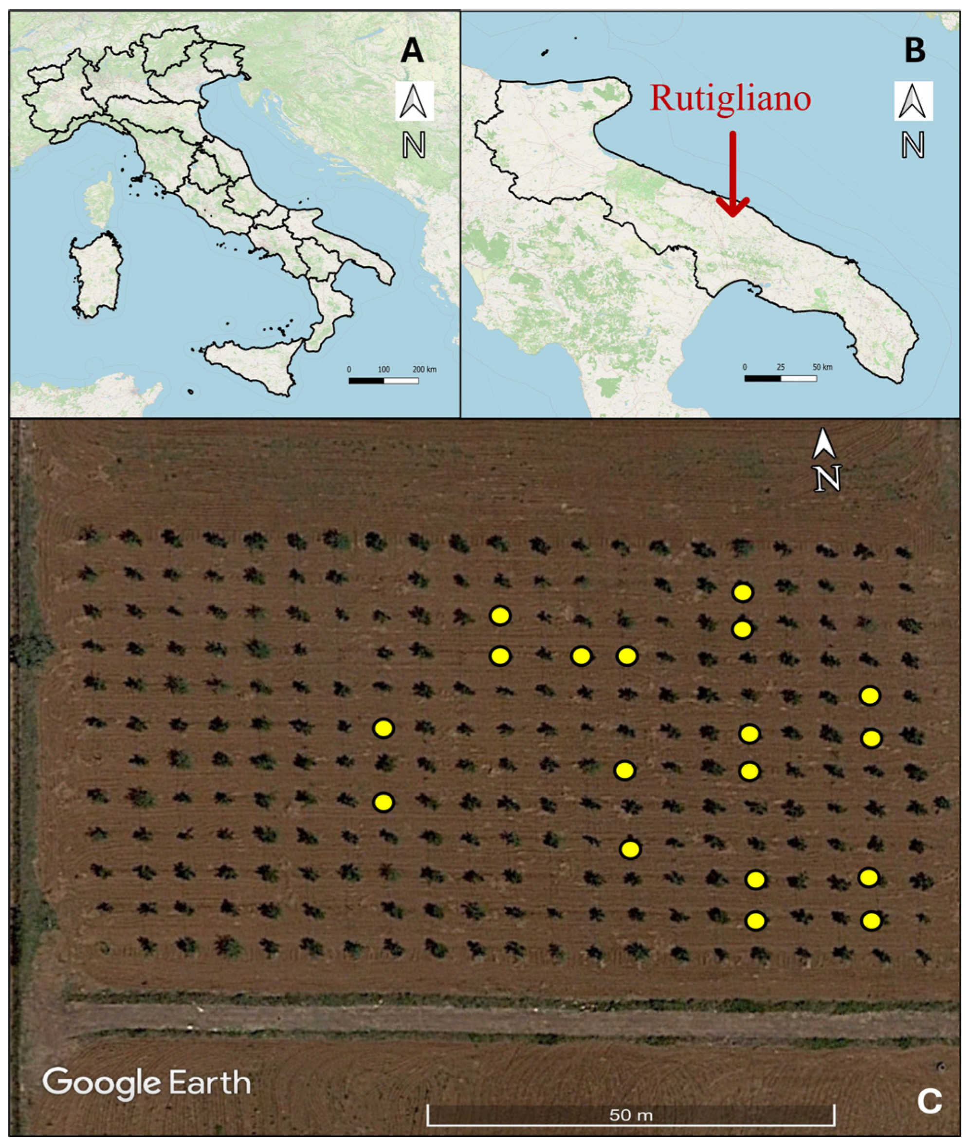
2.1. Experimental Site and Field Data
2.2. Satellite Images
2.3. Statistical Analysis and Machine Learning
3. Results
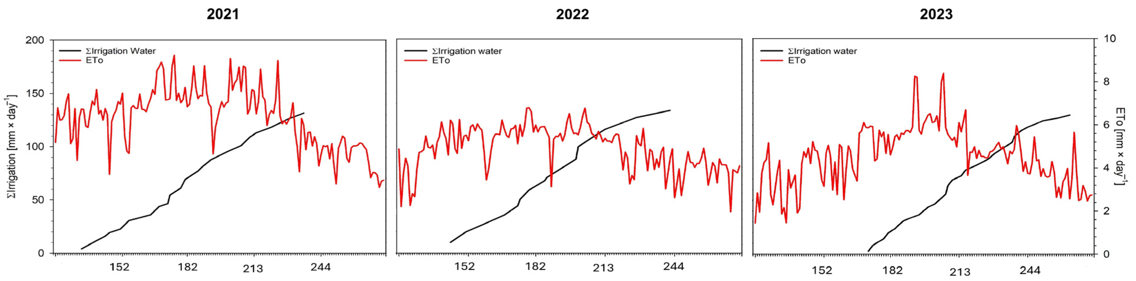
3.1. Field Data
3.2. Models’ Performance
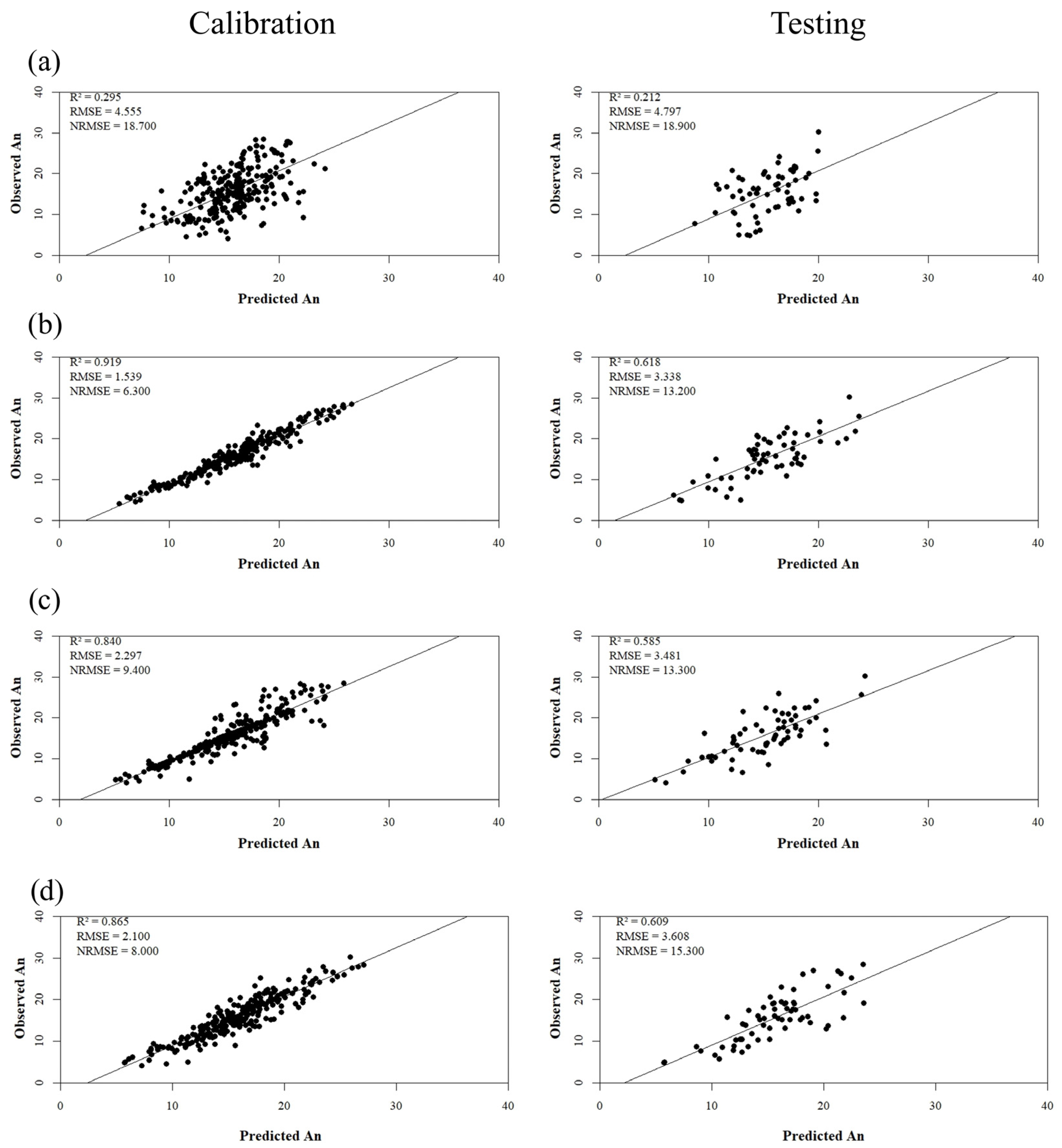
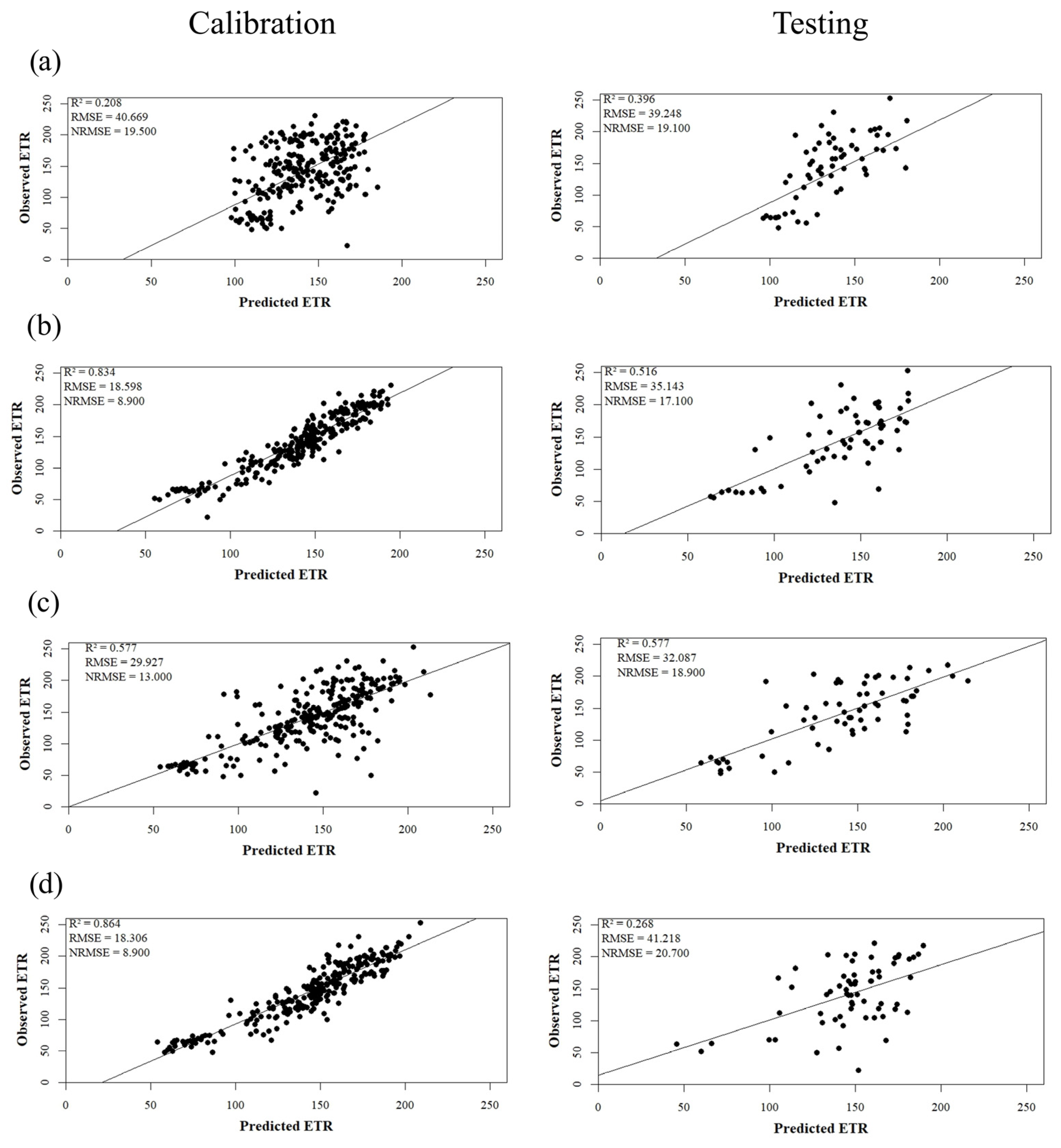
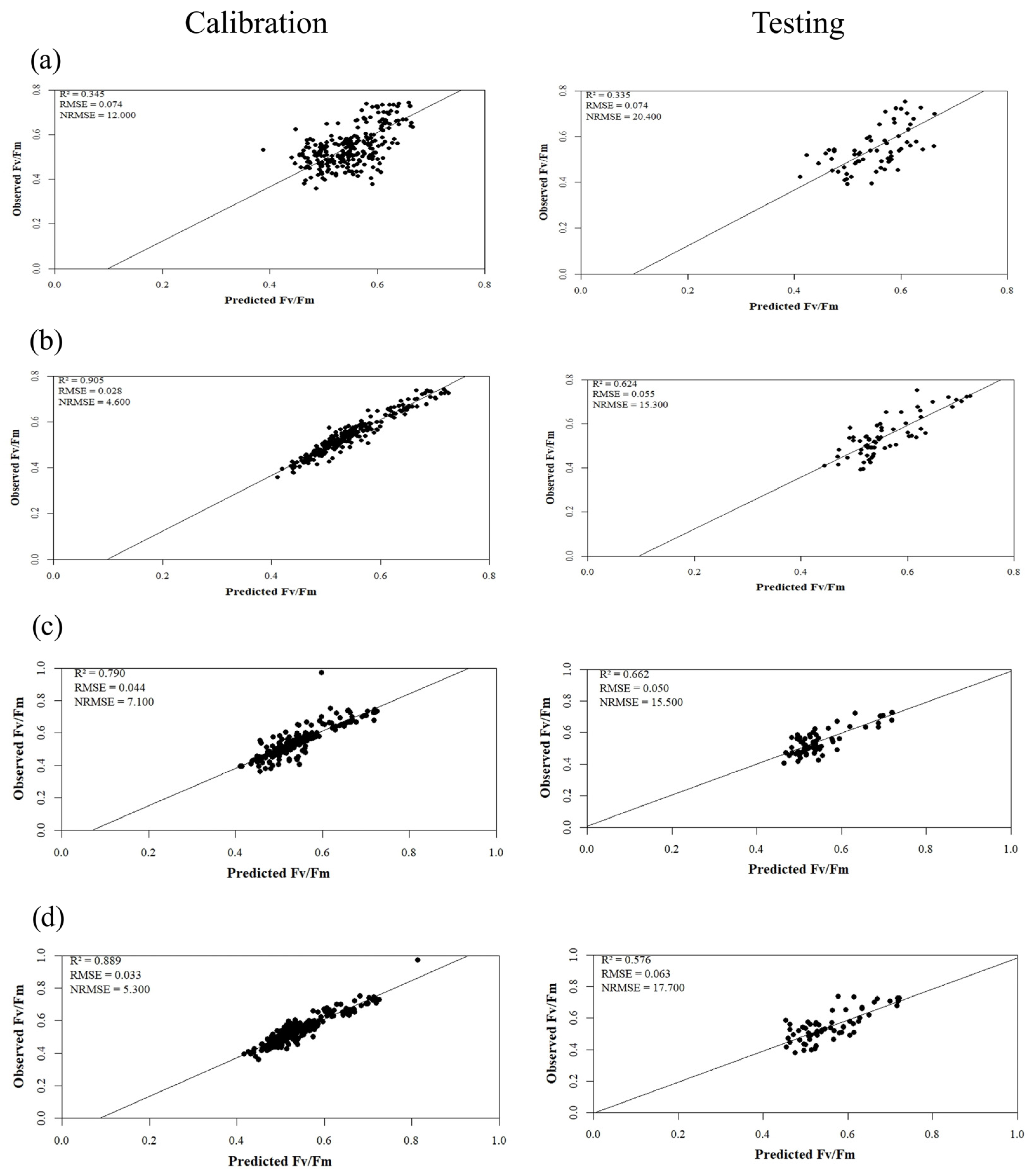
3.2.1. Physiology
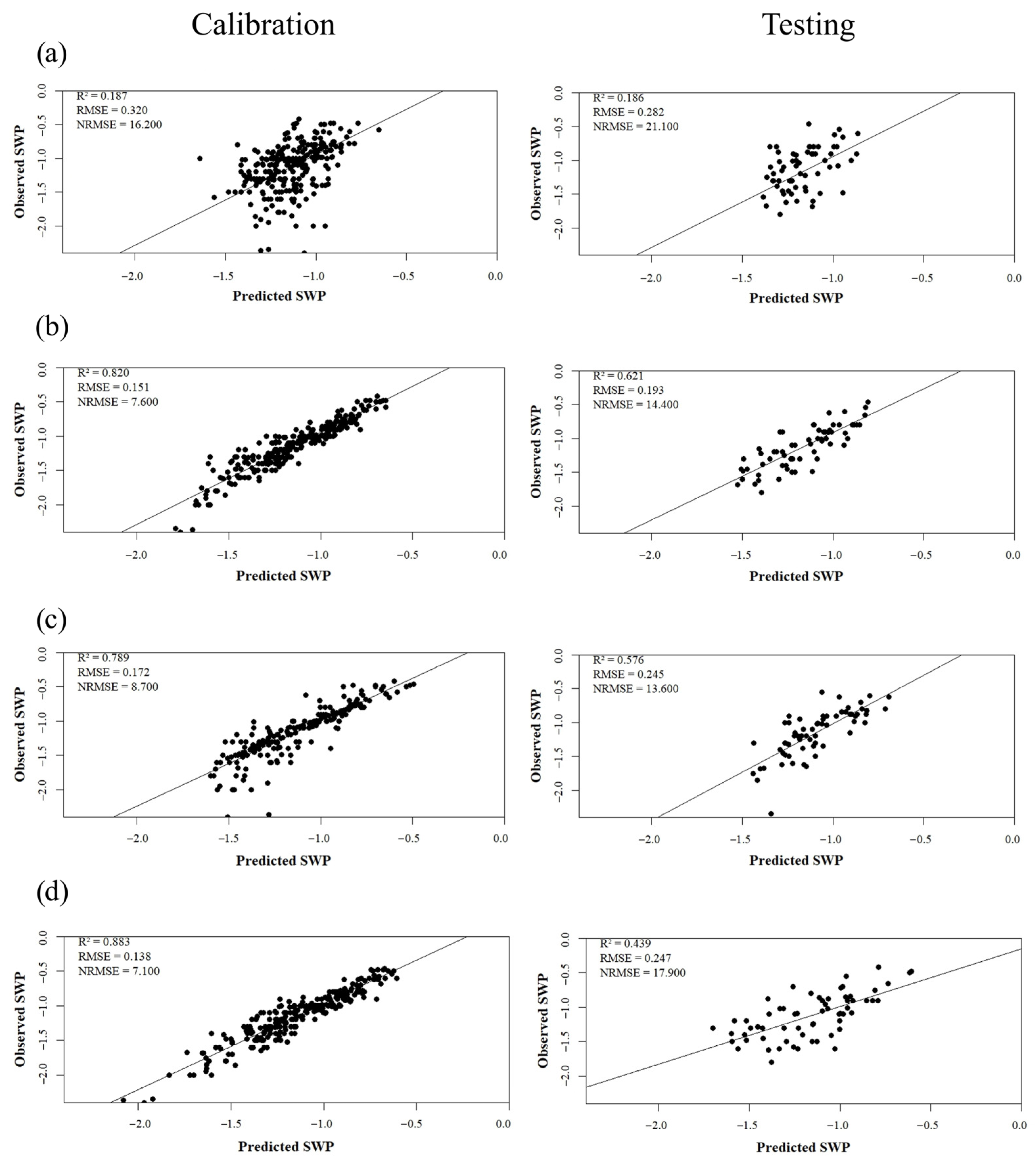
3.2.2. Stem Water Potential
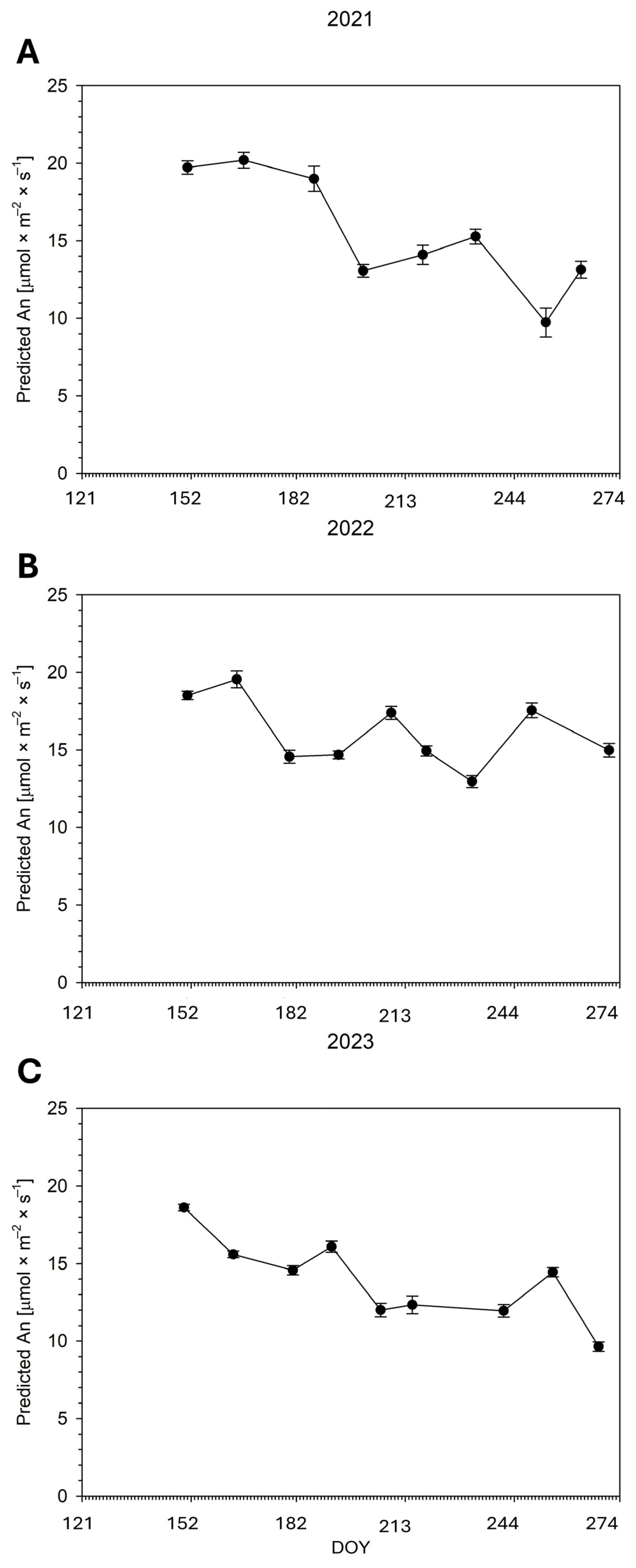
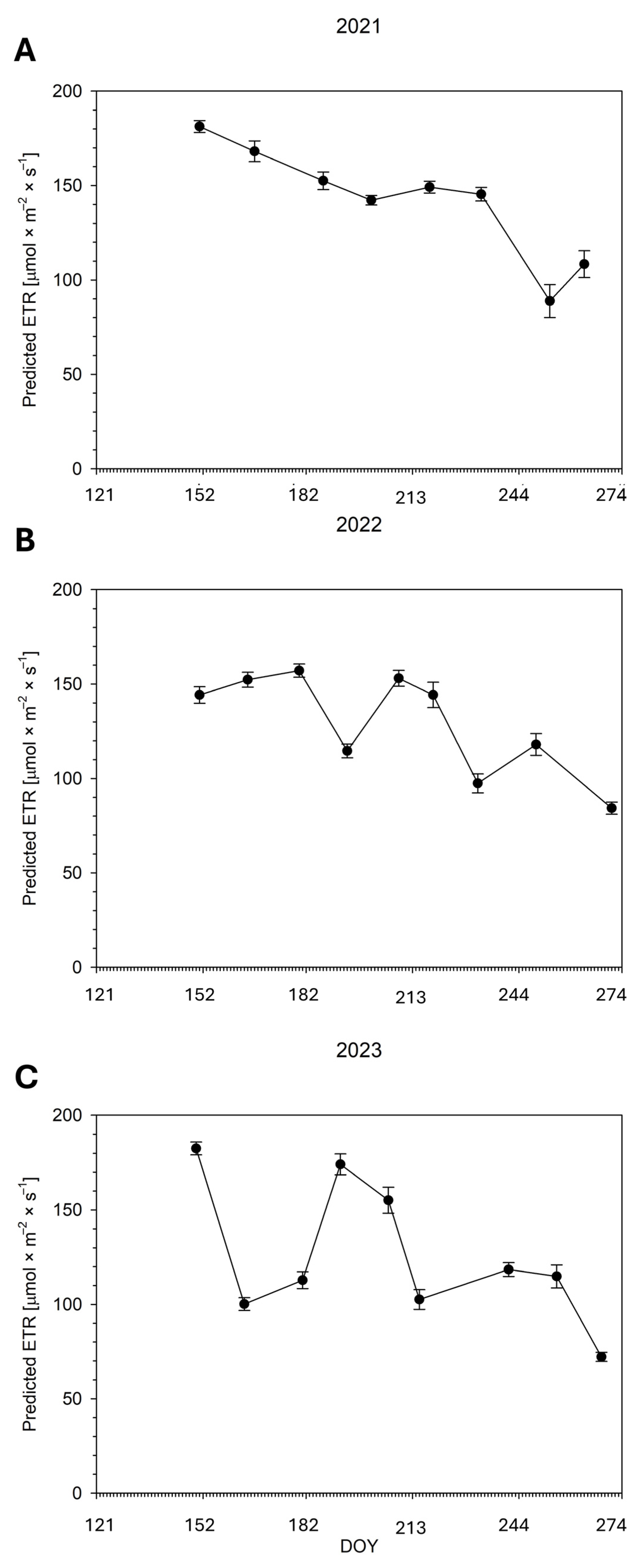
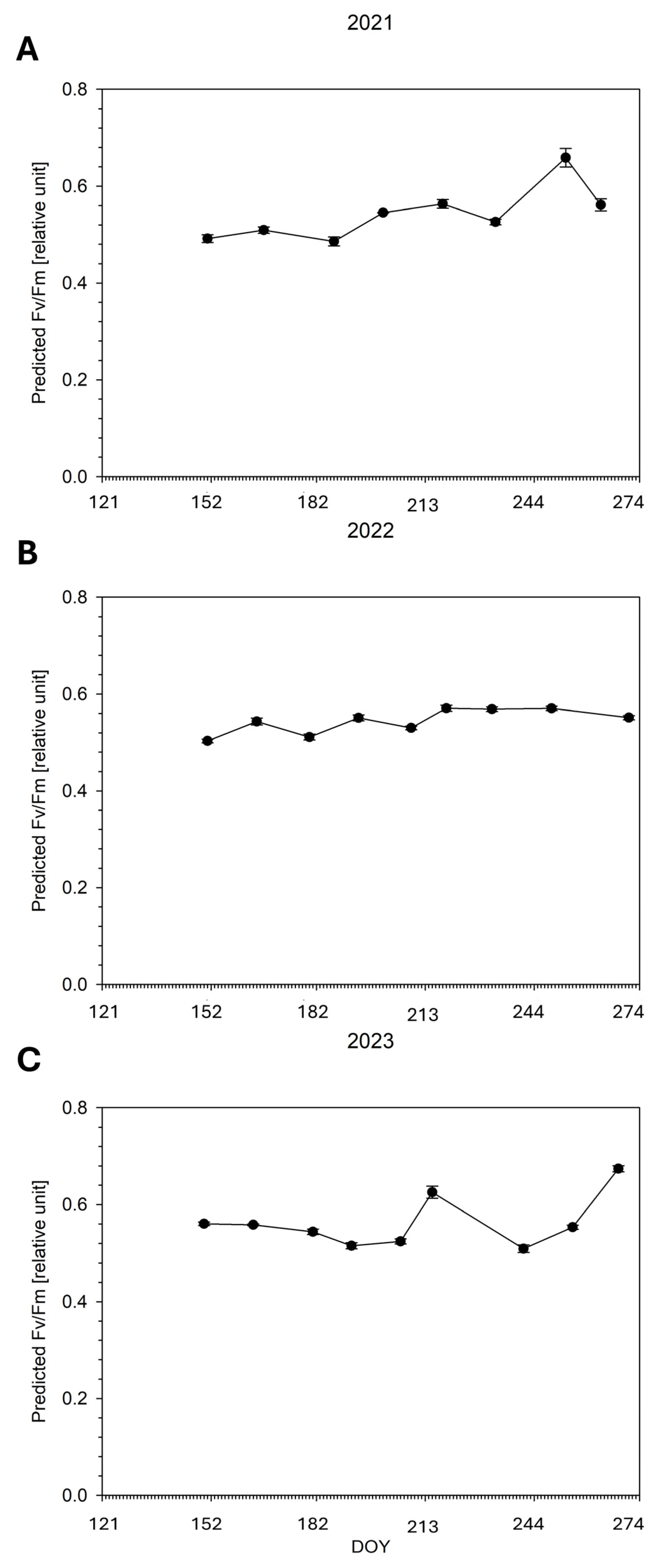
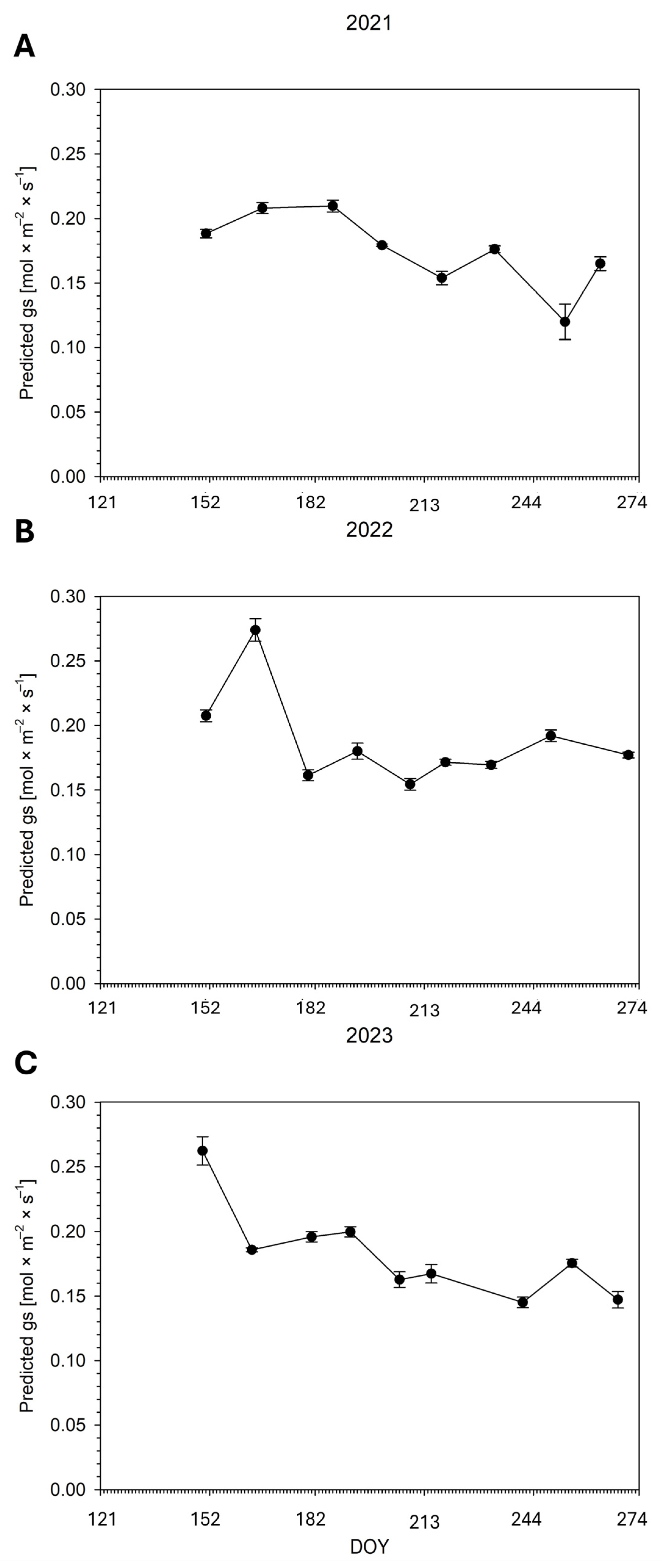
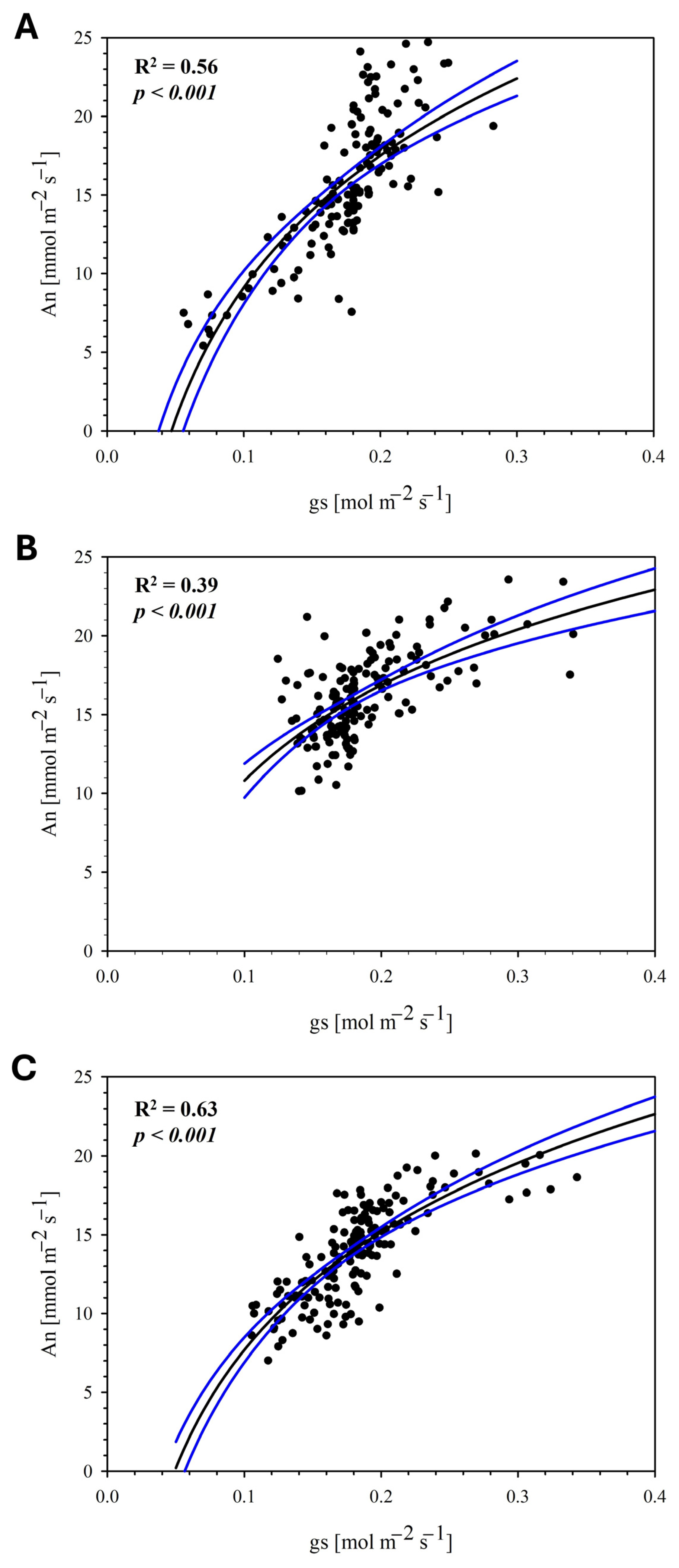
3.3. Predicted Physiology and Water Status
4. Discussion
5. Conclusions
Author Contributions
Funding
Data Availability Statement
Acknowledgments
Conflicts of Interest
References
- Costa, J.M.; Vaz, M.; Escalona, J.; Egipto, R.; Lopes, C.; Medrano, H.; Chaves, M.M. Modern Viticulture in Southern Europe: Vulnerabilities and Strategies for Adaptation to Water Scarcity. Agric. Water Manag. 2016, 164, 5–18. [Google Scholar] [CrossRef]
- Garofalo, S.P.; Intrigliolo, D.S.; Camposeo, S.; Ali, S.A.; Tedone, L.; Lopriore, G.; De Mastro, G.; Vivaldi, G.A. Agronomic Responses of Grapevines to an Irrigation Scheduling Approach Based on Continuous Monitoring of Soil Water Content. Agronomy 2023, 13, 2821. [Google Scholar] [CrossRef]
- Garofalo, S.P.; Giannico, V.; Costanza, L.; Alhajj Ali, S.; Camposeo, S.; Lopriore, G.; Pedrero Salcedo, F.; Vivaldi, G.A. Prediction of Stem Water Potential in Olive Orchards Using High-Resolution Planet Satellite Images and Machine Learning Techniques. Agronomy 2024, 14, 1. [Google Scholar] [CrossRef]
- De Souza, B.P.; Martinez, H.E.P.; de Carvalho, F.P.; Loureiro, M.E.; Sturião, W.P. Gas Exchanges and Chlorophyll Fluorescence of Young Coffee Plants Submitted to Water and Nitrogen Stresses. J. Plant Nutr. 2020, 43, 2455–2465. [Google Scholar] [CrossRef]
- Chen, C.I.; Lin, K.H.; Huang, M.Y.; Yang, C.K.; Lin, Y.H.; Hsueh, M.L.; Lee, L.H.; Wang, C.W. Photosynthetic Physiology Comparisons between No Tillage and Sod Culture of Citrus Farming in Different Seasons under Various Light Intensities. Agronomy 2021, 11, 1805. [Google Scholar] [CrossRef]
- Choné, X.; Van Leeuwen, C.; Dubourdieu, D.; Gaudillère, J.P. Stem Water Potential Is a Sensitive Indicator of Grapevine Water Status. Ann. Bot. 2001, 87, 477–483. [Google Scholar] [CrossRef]
- Hemati, A.; Moghiseh, E.; Amirifar, A.; Mofidi-Chelan, M.; Lajayer, B.A. Physiological Effects of Drought Stress in Plants. In Plant Stress Mitigators: Action and Application; Springer Nature: Singapore, 2022; pp. 113–124. [Google Scholar] [CrossRef]
- Toscano, S.; Franzoni, G.; Álvarez, S.; Álvarez, S. Drought Stress in Horticultural Plants. Drought Stress Hortic. Plants 2023, 232. [Google Scholar] [CrossRef]
- Naikwade, P.V. Plant Responses to Drought Stress: Morphological, Physiological, Molecular Approaches, and Drought Resistance. In Plant Metabolites under Environmental Stress; Apple Academic Press: Palm Bay, FL, USA, 2023; pp. 149–183. [Google Scholar] [CrossRef]
- Wu, J.; Wang, J.; Hui, W.; Zhao, F.; Wang, P.; Su, C.; Gong, W. Physiology of Plant Responses to Water Stress and Related Genes: A Review. Forests 2022, 13, 324. [Google Scholar] [CrossRef]
- Calvin, K. IPCC, 2023: Climate Change 2023: Synthesis Report. In Contribution of Working Groups I, II and III to the Sixth Assessment Report of the Intergovernmental Panel on Climate Change; Lee, H., Romero, J., Eds.; IPCC: Geneva, Switzerland, 2023. [Google Scholar]
- Van Leeuwen, C.; Destrac-Irvine, A.; Dubernet, M.; Duchêne, E.; Gowdy, M.; Marguerit, E.; Pieri, P.; Parker, A.; De Rességuier, L.; Ollat, N. An Update on the Impact of Climate Change in Viticulture and Potential Adaptations. Agronomy 2019, 9, 514. [Google Scholar] [CrossRef]
- Van Leeuwen, C.; Destrac-Irvine, A. Modified Grape Composition under Climate Change Conditions Requires Adaptations in the Vineyard. Oeno One 2017, 51, 147–154. [Google Scholar] [CrossRef]
- Gomez-Zavaglia, A.; Mejuto, J.C.; Simal-Gandara, J. Mitigation of Emerging Implications of Climate Change on Food Production Systems. Food Res. Int. 2020, 134, 109256. [Google Scholar] [CrossRef] [PubMed]
- Vuolo, F.; Essl, L.; Atzberger, C. Costs and Benefits of Satellite-Based Tools for Irrigation Management. Front. Environ. Sci. 2015, 3, 52. [Google Scholar] [CrossRef]
- Alhajj Ali, S.; Vivaldi, G.A.; Garofalo, S.P.; Costanza, L.; Camposeo, S. Land Suitability Analysis of Six Fruit Tree Species Immune/Resistant to Xylella Fastidiosa as Alternative Crops in Infected Olive-Growing Areas. Agronomy 2023, 13, 547. [Google Scholar] [CrossRef]
- Laroche-Pinel, E.; Duthoit, S.; Albughdadi, M.; Costard, A.D.; Rousseau, J.; Chéret, V.; Clenet, H. Towards Vine Water Status Monitoring on a Large Scale Using Sentinel-2 Images. Remote Sens. 2021, 13, 1837. [Google Scholar] [CrossRef]
- Virnodkar, S.S.; Pachghare, V.K.; Patil, V.C.; Jha, S.K. Remote Sensing and Machine Learning for Crop Water Stress Determination in Various Crops: A Critical Review. Precis. Agric. 2020, 21, 1121–1155. [Google Scholar] [CrossRef]
- Pallathadka, H.; Mustafa, M.; Sanchez, D.T.; Sekhar Sajja, G.; Gour, S.; Naved, M. Impact of Machine Learning on Management, Healthcare and Agriculture. Mater. Today Proc. 2023, 80, 2803–2806. [Google Scholar] [CrossRef]
- Lee, H.; Wang, J.; Leblon, B. Using Linear Regression, Random Forests, and Support Vector Machine with Unmanned Aerial Vehicle Multispectral Images to Predict Canopy Nitrogen Weight in Corn. Remote Sens. 2020, 12, 2071. [Google Scholar] [CrossRef]
- Gammermann, A. Support Vector Machine Learning Algorithm and Transduction. Comput. Stat. 2000, 15, 31–39. [Google Scholar] [CrossRef]
- Mariadass, D.A.L.; Moung, E.G.; Sufian, M.M.; Farzamnia, A. Extreme Gradient Boosting (XGBoost) Regressor and Shapley Additive Explanation for Crop Yield Prediction in Agriculture. In Proceedings of the 2022 12th International Conference on Computer and Knowledge Engineering, ICCKE 2022, Mashhad, Iran, 17–18 November 2022; pp. 219–224. [Google Scholar] [CrossRef]
- Noorunnahar, M.; Chowdhury, A.H.; Arefeen, F.; Id, M. A Tree Based EXtreme Gradient Boosting (XGBoost) Machine Learning Model to Forecast the Annual Rice Production in Bangladesh. PLoS ONE 2023, 18, e0283452. [Google Scholar] [CrossRef] [PubMed]
- Tian, Y.; Xu, Y.P.; Wang, G. Agricultural Drought Prediction Using Climate Indices Based on Support Vector Regression in Xiangjiang River Basin. Sci. Total Environ. 2018, 622–623, 710–720. [Google Scholar] [CrossRef] [PubMed]
- Ellsäßer, F.; Röll, A.; Ahongshangbam, J.; Waite, P.A.; Hendrayanto; Schuldt, B.; Hölscher, D. Predicting Tree Sap Flux and Stomatal Conductance from Drone-Recorded Surface Temperatures in a Mixed Agroforestry System—A Machine Learning Approach. Remote Sens. 2020, 12, 4070. [Google Scholar] [CrossRef]
- López-García, P.; Intrigliolo, D.; Moreno, M.A.; Martínez-Moreno, A.; Ortega, J.F.; Pérez-Álvarez, E.P.; Ballesteros, R. Machine Learning-Based Processing of Multispectral and RGB UAV Imagery for the Multitemporal Monitoring of Vineyard Water Status. Agronomy 2022, 12, 2122. [Google Scholar] [CrossRef]
- Pedrero, F.; Camposeo, S.; Pace, B.; Cefola, M.; Vivaldi, G.A. Use of Reclaimed Wastewater on Fruit Quality of Nectarine in Southern Italy. Agric. Water Manag. 2018, 203, 186–192. [Google Scholar] [CrossRef]
- Climate-Data 2024. Available online: https://en.climate-data.org/ (accessed on 3 May 2024).
- Allen, R.G.; Pereira, L.S.; Raes, D.; Smith, M. Crop Evapotranspiration-Guidelines for Computing Crop Water Requirements-FAO Irrigation and Drainage Paper 56; FAO: Geneva, Switzerland, 1998. [Google Scholar]
- Tomasella, M.; Calderan, A.; Mihelčič, A.; Petruzzellis, F.; Braidotti, R.; Natale, S.; Lisjak, K.; Sivilotti, P.; Nardini, A. Best Procedures for Leaf and Stem Water Potential Measurements in Grapevine: Cultivar and Water Status Matter. Plants 2023, 12, 2412. [Google Scholar] [CrossRef] [PubMed]
- Suter, B.; Triolo, R.; Pernet, D.; Dai, Z.; Van Leeuwen, C. Modeling Stem Water Potential by Separating the Effects of Soil Water Availability and Climatic Conditions on Water Status in Grapevine (Vitis vinifera L.). Front. Plant Sci. 2019, 10, 495956. [Google Scholar] [CrossRef] [PubMed]
- Planet Imagery Product Specifications. Available online: https://www.planet.com/products/satellite-imagery-of-earth/ (accessed on 8 May 2024).
- RStudio Team. RStudio 2020. RStudio: Integrated development for R (Boston, MA: RStudio, PBC). Available online: http://www.rstudio.com/ (accessed on 25 June 2024).
- Sobhana, M.; Smitha Chowdary, C.; Indira, D.N.V.S.L.S.; Kumar, K.K. CROPUP—A Crop Yield Prediction and Recommendation System with Geographical Data Using DNN and XGBoost. Int. J. Recent Innov. Trends Comput. Commun. 2022, 10, 53–62. [Google Scholar] [CrossRef]
- Silva, J.V.; van Heerwaarden, J.; Reidsma, P.; Laborte, A.G.; Tesfaye, K.; van Ittersum, M.K. Big Data, Small Explanatory and Predictive Power: Lessons from Random Forest Modeling of on-Farm Yield Variability and Implications for Data-Driven Agronomy. Field Crops Res. 2023, 302, 109063. [Google Scholar] [CrossRef] [PubMed]
- Belgiu, M.; Drăgu, L. Random Forest in Remote Sensing: A Review of Applications and Future Directions. ISPRS J. Photogramm. Remote Sens. 2016, 114, 24–31. [Google Scholar] [CrossRef]
- Salcedo-Sanz, S.; Rojo-Álvarez, J.L.; Martínez-Ramón, M.; Camps-Valls, G. Support Vector Machines in Engineering: An Overview. Wiley Interdiscip. Rev. Data Min. Knowl. Discov. 2014, 4, 234–267. [Google Scholar] [CrossRef]
- Kuhn, M. Building Predictive Models in R Using the Caret Package. J. Stat. Softw. 2008, 28, 1–26. [Google Scholar] [CrossRef]
- Hijmans, R.J.; van Etten, J. R Package “raster”, Version 3.6-26. 2023. Available online: https://cran.r-project.org/web/packages/raster/raster.pdf (accessed on 26 June 2024).
- Chen, D.; Zhang, J.; Zhang, Z.; Wan, X.; Hu, J. Analyzing the Effect of Light on Lettuce Fv/Fm and Growth by Machine Learning. Sci. Hortic. 2022, 306, 111444. [Google Scholar] [CrossRef]
- Wu, Q.; Zhang, Y.; Xie, M.; Zhao, Z.; Yang, L.; Liu, J.; Hou, D.; Wang, C.; Wu, Q.; Zhang, Y.; et al. Estimation of Fv/Fm in Spring Wheat Using UAV-Based Multispectral and RGB Imagery with Multiple Machine Learning Methods. Agronomy 2023, 13, 1003. [Google Scholar] [CrossRef]
- Jutamanee, K.; Onnom, S. Improving Photosynthetic Performance and Some Fruit Quality Traits in Mango Trees by Shading. Photosynthetica 2016, 54, 542–550. [Google Scholar] [CrossRef]
- McArtney, S.J.; Obermiller, J.D.; Arellano, C. Comparison of the Effects of Metamitron on Chlorophyll Fluorescence and Fruit Set in Apple and Peach. HortScience 2012, 47, 509–514. [Google Scholar] [CrossRef]
- Bartold, M.; Kluczek, M. Estimating of Chlorophyll Fluorescence Parameter Fv/Fm for Plant Stress Detection at Peatlands under Ramsar Convention with Sentinel-2 Satellite Imagery. Ecol. Inform. 2024, 81, 102603. [Google Scholar] [CrossRef]
- Navarro Cerrillo, R.M.; Ariza, D.; Maldonado Rodriguez, R. Chlorophyll Fluorescence Response in Five Provenances of Pinus Pinus Halepensis Mill to Drought Stress. Cuad. Soc. Española Cienc. For. 2004, 17, 69–74. [Google Scholar]
- Garofalo, S.P.; Giannico, V.; Lorente, B.; Vivaldi, G.A.; Jose, A. Predicting Carob Tree Physiological Parameters under Different Irrigation Systems Using Random Forest and Planet Satellite Images. Front. Plant Sci. 2024, 15, 1302435. [Google Scholar] [CrossRef] [PubMed]
- Zhang, X.Y.; Huang, Z.; Su, X.; Siu, A.; Song, Y.; Zhang, D.; Fang, Q. Machine Learning Models for Net Photosynthetic Rate Prediction Using Poplar Leaf Phenotype Data. PLoS ONE 2020, 15, e0228645. [Google Scholar] [CrossRef]
- Fu, P.; Meacham-Hensold, K.; Guan, K.; Bernacchi, C.J. Hyperspectral Leaf Reflectance as Proxy for Photosynthetic Capacities: An Ensemble Approach Based on Multiple Machine Learning Algorithms. Front. Plant Sci. 2019, 10, 454448. [Google Scholar] [CrossRef] [PubMed]
- Wu, T.; Zhang, W.; Wu, S.; Cheng, M.; Qi, L.; Shao, G.; Jiao, X. Retrieving Rice (Oryza sativa L.) Net Photosynthetic Rate from UAV Multispectral Images Based on Machine Learning Methods. Front Plant Sci 2023, 13, 1088499. [Google Scholar] [CrossRef] [PubMed]
- Xie, J.; Chen, Y.; Yu, Z.; Wang, J.; Liang, G.; Gao, P.; Sun, D.; Wang, W.; Shu, Z.; Yin, D.; et al. Estimating Stomatal Conductance of Citrus under Water Stress Based on Multispectral Imagery and Machine Learning Methods. Front. Plant Sci. 2023, 14, 1054587. [Google Scholar] [CrossRef] [PubMed]
- Zhou, J.J.; Zhang, Y.H.; Han, Z.M.; Liu, X.Y.; Jian, Y.F.; Hu, C.G.; Dian, Y.Y. Evaluating the Performance of Hyperspectral Leaf Reflectance to Detect Water Stress and Estimation of Photosynthetic Capacities. Remote Sens. 2021, 13, 2160. [Google Scholar] [CrossRef]
- Jones, H.G. Stomatal Control of Photosynthesis and Transpiration. J. Exp. Bot. 1998, 49, 387–398. [Google Scholar] [CrossRef]
- Medrano, H.; Flexas, J.; Galmés, J. Variability in Water Use Efficiency at the Leaf Level among Mediterranean Plants with Different Growth Forms. Plant Soil 2009, 317, 17–29. [Google Scholar] [CrossRef]
- Yang, Z.; Tian, J.; Wang, Z.; Feng, K. Monitoring the Photosynthetic Performance of Grape Leaves Using a Hyperspectral-Based Machine Learning Model. Eur. J. Agron. 2022, 140, 126589. [Google Scholar] [CrossRef]
- Genty, B.; Briantais, J.M.; Baker, N.R. The Relationship between the Quantum Yield of Photosynthetic Electron Transport and Quenching of Chlorophyll Fluorescence. Biochim. Et Biophys. Acta (BBA)-Gen. Subj. 1989, 990, 87–92. [Google Scholar] [CrossRef]
- Tian, Y.; Sacharz, J.; Ware, M.A.; Zhang, H.; Ruban, A.V. Effects of Periodic Photoinhibitory Light Exposure on Physiology and Productivity of Arabidopsis Plants Grown under Low Light. J. Exp. Bot. 2017, 68, 4249–4262. [Google Scholar] [CrossRef] [PubMed]
- Gu, J.; Zhou, Z.; Li, Z.; Chen, Y.; Wang, Z.; Zhang, H.; Yang, J. Photosynthetic Properties and Potentials for Improvement of Photosynthesis in Pale Green Leaf Rice under High Light Conditions. Front. Plant Sci. 2017, 8, 235715. [Google Scholar] [CrossRef] [PubMed]
- Takahashi, S.; Badger, M.R. Photoprotection in Plants: A New Light on Photosystem II Damage. Trends Plant Sci. 2011, 16, 53–60. [Google Scholar] [CrossRef] [PubMed]
- Murata, N.; Takahashi, S.; Nishiyama, Y.; Allakhverdiev, S.I. Photoinhibition of Photosystem II under Environmental Stress. Biochim. Et Biophys. Acta (BBA)-Bioenerg. 2007, 1767, 414–421. [Google Scholar] [CrossRef] [PubMed]
- Flexas, J.; Bota, J.; Galmés, J.; Medrano, H.; Ribas-Carbó, M. Keeping a Positive Carbon Balance under Adverse Conditions: Responses of Photosynthesis and Respiration to Water Stress. Physiol. Plant 2006, 127, 343–352. [Google Scholar] [CrossRef]
- Shi, B.; Yuan, Y.; Zhuang, T.; Xu, X.; Schmidhalter, U.; Ata-UI-Karim, S.T.; Zhao, B.; Liu, X.; Tian, Y.; Zhu, Y.; et al. Improving Water Status Prediction of Winter Wheat Using Multi-Source Data with Machine Learning. Eur. J. Agron. 2022, 139, 126548. [Google Scholar] [CrossRef]
- Tang, Z.; Jin, Y.; Alsina, M.M.; McElrone, A.J.; Bambach, N.; Kustas, W.P. Vine Water Status Mapping with Multispectral UAV Imagery and Machine Learning. Irrig. Sci. 2022, 40, 715–730. [Google Scholar] [CrossRef]
- Ohana-Levi, N.; Munitz, S.; Netzer, Y. Grapevine Stem Water Potential Seasonal Curves: Response to Meteorological Conditions, and Association to Yield and Red Wine Quality. Agric. For. Meteorol. 2023, 342, 109755. [Google Scholar] [CrossRef]
- Olivo, N.; Girona, J.; Marsal, J. Seasonal Sensitivity of Stem Water Potential to Vapour Pressure Deficit in Grapevine. Irrig. Sci. 2009, 27, 175–182. [Google Scholar] [CrossRef]
- Teixeira, A.H.d.C.; de Miranda, F.R.; Leivas, J.F.; Pacheco, E.P.; Garçon, E.A.M. Water Productivity Assessments for Dwarf Coconut by Using Landsat 8 Images and Agrometeorological Data. ISPRS J. Photogramm. Remote Sens. 2019, 155, 150–158. [Google Scholar] [CrossRef]
- Helman, D.; Bahat, I.; Netzer, Y.; Ben-Gal, A.; Alchanatis, V.; Peeters, A.; Cohen, Y. Using Time Series of High-Resolution Planet Satellite Images to Monitor Grapevine Stem Water Potential in Commercial Vineyards. Remote Sens. 2018, 10, 1615. [Google Scholar] [CrossRef]
- Lin, C.; Jin, Z.; Mulla, D.; Ghosh, R.; Guan, K.; Kumar, V.; Cai, Y. Toward Large-Scale Mapping of Tree Crops with High-Resolution Satellite Imagery and Deep Learning Algorithms: A Case Study of Olive Orchards in Morocco. Remote Sens. 2021, 13, 1740. [Google Scholar] [CrossRef]
- Pettorelli, N.; Vik, J.O.; Mysterud, A.; Gaillard, J.M.; Tucker, C.J.; Stenseth, N.C. Using the Satellite-Derived NDVI to Assess Ecological Responses to Environmental Change. Trends Ecol. Evol. 2005, 20, 503–510. [Google Scholar] [CrossRef] [PubMed]
- Lin, Y.; Zhu, Z.; Guo, W.; Sun, Y.; Yang, X.; Kovalskyy, V. Continuous Monitoring of Cotton Stem Water Potential Using Sentinel-2 Imagery. Remote Sens. 2020, 12, 1176. [Google Scholar] [CrossRef]
- Loannis, N.; Alexandridis, T.K.; Moshou, D.; Pantazi, X.E.; Tamouridou, A.A.; Kozhukh, D.; Castef, F.; Lagopodi, A.; Zartaloudis, Z.; Mourelatos, S.; et al. Olive Trees Stress Detection Using Sentinel-2 Images. In Proceedings of the IEEE International Geoscience and Remote Sensing Symposium, Yokohama, Japan, 28 July–2 August 2019. [Google Scholar]
- Jamshidi, S.; Zand-Parsa, S.; Niyogi, D. Assessing Crop Water Stress Index of Citrus Using In-Situ Measurements, Landsat, and Sentinel-2 Data. Int. J. Remote Sens. 2021, 42, 1893–1916. [Google Scholar] [CrossRef]
- Lo Bianco, R.; Pisciotta, A.; Manfrini, L.; Fallahi, E.; Borgogno-Mondino, E.; Farbo, A.; Novello, V.; De Palma, L. A Fast Regression-Based Approach to Map Water Status of Pomegranate Orchards with Sentinel 2 Data. Horticulturae 2022, 8, 759. [Google Scholar] [CrossRef]
- Lakso, A.N.; Santiago, M.; Stroock, A.D. Monitoring Stem Water Potential with an Embedded Microtensiometer to Inform Irrigation Scheduling in Fruit Crops. Horticulturae 2022, 8, 1207. [Google Scholar] [CrossRef]
- Noun, G.; Lo Cascio, M.; Spano, D.; Marras, S.; Sirca, C. Plant-Based Methodologies and Approaches for Estimating Plant Water Status of Mediterranean Tree Species: A Semi-Systematic Review. Agronomy 2022, 12, 2127. [Google Scholar] [CrossRef]
- Maldera, F.; Garofalo, S.P.; Camposeo, S. Ecophysiological Recovery of Micropropagated Olive Cultivars: Field Research in an Irrigated Super-High-Density Orchard. Agronomy 2024, 14, 1560. [Google Scholar] [CrossRef]
- Gonzalez-Dugo, V.; Zarco-Tejada, P.; Nicolás, E.; Nortes, P.A.; Alarcón, J.J.; Intrigliolo, D.S.; Fereres, E. Using high resolution UAV thermal imagery to assess the variability in the water status of five fruit tree species within a commercial orchard. Precis. Agric. 2013, 14, 660–678. [Google Scholar] [CrossRef]


| Parameter | |
|---|---|
| Sand (g·100 g−1) | 21 |
| Silt (g·100 g−1) | 37 |
| Clay (g·100 g−1) | 42 |
| E.C. (dS·m−1) | 0.6 |
| SOC (g·kg−1) | 14 |
| Parameter | Year | Mean | s.d. | Median | Min | Max | |
|---|---|---|---|---|---|---|---|
| An | 2021 | 11.09 | 4.92 | 10.69 | 4.12 | 25.15 | c |
| 2022 | 18.58 | 4.56 | 18.13 | 9.30 | 30.21 | a | |
| 2023 | 14.42 | 4.64 | 14.57 | 4.53 | 26.11 | b | |
| ETR | 2021 | 116.86 | 54.88 | 126.96 | 22.54 | 219.20 | b |
| 2022 | 151.20 | 38.40 | 153.61 | 47.65 | 253.23 | a | |
| 2023 | 140.01 | 47.31 | 145.63 | 47.75 | 221.56 | a | |
| Fv/Fm | 2021 | 0.59 | 0.13 | 0.63 | 0.39 | 0.97 | a |
| 2022 | 0.52 | 0.05 | 0.52 | 0.36 | 0.70 | c | |
| 2023 | 0.55 | 0.09 | 0.53 | 0.39 | 0.75 | b | |
| gs | 2021 | 0.12 | 0.07 | 0.10 | 0.03 | 0.38 | c |
| 2022 | 0.20 | 0.07 | 0.19 | 0.07 | 0.47 | a | |
| 2023 | 0.18 | 0.04 | 0.18 | 0.08 | 0.31 | b | |
| SWP | 2021 | −1.33 | 0.26 | −1.30 | −2.00 | −0.8 | b |
| 2022 | −1.14 | 0.27 | −1.1 | −2.00 | −0.70 | a | |
| 2023 | −1.16 | 0.39 | −1.02 | −2.40 | −0.56 | a | |
| An | overall | 15.62 | 5.42 | 15.47 | 4.12 | 30.21 | |
| ETR | 140.57 | 46.75 | 144.07 | 22.54 | 253.23 | ||
| Fv/Fm | 0.18 | 0.07 | 0.17 | 0.03 | 0.47 | ||
| gs | 0.54 | 0.09 | 0.53 | 0.36 | 0.97 | ||
| SWP | −1.13 | 0.34 | −1.10 | −2.40 | −0.42 |
Disclaimer/Publisher’s Note: The statements, opinions and data contained in all publications are solely those of the individual author(s) and contributor(s) and not of MDPI and/or the editor(s). MDPI and/or the editor(s) disclaim responsibility for any injury to people or property resulting from any ideas, methods, instructions or products referred to in the content. |
© 2024 by the authors. Licensee MDPI, Basel, Switzerland. This article is an open access article distributed under the terms and conditions of the Creative Commons Attribution (CC BY) license (https://creativecommons.org/licenses/by/4.0/).
Share and Cite
Campi, P.; Modugno, A.F.; De Carolis, G.; Pedrero Salcedo, F.; Lorente, B.; Garofalo, S.P. A Machine Learning Approach to Monitor the Physiological and Water Status of an Irrigated Peach Orchard under Semi-Arid Conditions by Using Multispectral Satellite Data. Water 2024, 16, 2224. https://doi.org/10.3390/w16162224
Campi P, Modugno AF, De Carolis G, Pedrero Salcedo F, Lorente B, Garofalo SP. A Machine Learning Approach to Monitor the Physiological and Water Status of an Irrigated Peach Orchard under Semi-Arid Conditions by Using Multispectral Satellite Data. Water. 2024; 16(16):2224. https://doi.org/10.3390/w16162224
Chicago/Turabian StyleCampi, Pasquale, Anna Francesca Modugno, Gabriele De Carolis, Francisco Pedrero Salcedo, Beatriz Lorente, and Simone Pietro Garofalo. 2024. "A Machine Learning Approach to Monitor the Physiological and Water Status of an Irrigated Peach Orchard under Semi-Arid Conditions by Using Multispectral Satellite Data" Water 16, no. 16: 2224. https://doi.org/10.3390/w16162224
APA StyleCampi, P., Modugno, A. F., De Carolis, G., Pedrero Salcedo, F., Lorente, B., & Garofalo, S. P. (2024). A Machine Learning Approach to Monitor the Physiological and Water Status of an Irrigated Peach Orchard under Semi-Arid Conditions by Using Multispectral Satellite Data. Water, 16(16), 2224. https://doi.org/10.3390/w16162224