Estimating Increased Transient Water Storage with Increases in Beaver Dam Activity

Abstract

Dam building by beaver (Castor spp.) slows water movement through montane valleys, increasing transient water storage and the diversity of residence times. In some cases, water storage created by beaver dam construction is correlated to changes in streamflow magnitude and timing. However, the total amount of additional surface and groundwater storage that beaver dams may create (and, thus, their maximum potential impact on streamflow) has not been contextualized in the water balance of larger river basins. We estimate the potential transient water storage increases that could be created at 5, 25, 50, and 100% of maximum modeled beaver dam capacity in the Bear River basin, USA, by adapting the height above nearest drainage (HAND) algorithm to spatially estimate surface water storage. Surface water storage estimates were combined with the MODFLOW groundwater model to estimate potential increases in groundwater storage throughout the basin. We tested four scenarios to estimate potential transient water storage increases resulting from the construction of 1179 to 34,897 beaver dams, and estimated surface water storage to range from 57.5 to 72.8 m³ per dam and groundwater storage to range from 182.2 to 313.3 m³ per dam. Overall, we estimate that beaver dam construction could increase transient water storage by up to 10.38 million m³ in the Bear River basin. We further contextualize beaver dam-related water storage increases with streamflow, reservoir, and snowpack volumes.

1. Introduction

In many regions of the western United States, storage of seasonal precipitation is essential to meet water demand through drier periods. In these regions, the key reservoirs of water storage are snowpack and groundwater, with human-made reservoirs representing a distant third source [1]. Predictions and observations of warmer winters, and the resulting loss of snowpack, present water storage issues in these regions [1,2,3], and when this is combined with public sentiment against the construction of additional human-made reservoirs, investigating other solutions for storing water is required. One potential source of water storage could come from increased beaver dam construction. In the act of dam construction, beavers (Castor spp.) create both surface and subsurface (i.e., groundwater) water storage [4,5,6]. Because beavers have been heavily extirpated, many riverscapes have the potential to support many more beaver dams than currently exist and, thus, the potential to increase transient water storage [7,8].

In lotic environments, beaver dams diversify the residence times and complicate the flow paths of water by direct ponding, diverting flow onto floodplains, increasing groundwater infiltration, and altering evapotranspiration (ET) rates [6,9,10,11]. Generally, beaver dam construction increases a riverscape’s water storage potential [4,6,11,12]. The cumulative hydrologic impacts of beaver dams can range from increased ET and suppressed baseflow [11,13] to the attenuation of flood peaks, an increased baseflow downstream of beaver dams [4,14,15], and increased water inundation at the landscape scale [16]. Because of these potential environmental impacts, some have suggested that beaver dams could convert some streams from intermittent to perennial flow or maintain perennial water sources during drought conditions [17,18]. Indeed, many beaver relocation and beaver-based restoration efforts cite increased water quantity as a desired outcome [12]. However, while the effects of beaver dam construction on streamflow and water storage have been documented at the reach scale, the magnitude to which beaver dams may impact stream hydrology at larger extents has not been quantified [12].

The maximum effect of beaver dams on streamflow for a watershed can be conceptualized with a simple water balance, where surface water discharge (Q) is equal to precipitation (P) minus ET, minus changes in water storage (∆S).

$$Q = P - ET - ∆S$$

In a scenario where P and ET are constant, when ∆S is negative (i.e., water is leaving upstream storage reservoirs), Q increases, and when ∆S is positive (i.e., water is filling upstream storage reservoirs), Q decreases.

In this simple example, ∆S represents all water storage reservoirs (both above and below ground) in a watershed. Thus, the degree to which beaver dams may alter streamflow depends on the degree to which they may increase total transient water storage in a watershed by directly ponding water [5] and raising groundwater levels [9,19]. Greater total water storage in a watershed increases the potential for ∆S fluctuations (i.e., greater Q decreases when ∆S > 0 and greater Q increases when ∆S < 0) [4,14]. It is important to note that transient water storage increases are representative of a maximum streamflow effect (when considering potential streamflow increases), because beaver dam construction may also initiate changes to ET by increasing the area of open water, making more water available to plant roots, or causing tree mortality by inundation.

The amount of transient water storage beaver dams may create is dependent upon the size and density (or frequency) of the dams and local topography and geology [5]. Pond sizes are constrained by local topography, hydrology, and dam dimensions [20,21,22]. The surface volumes of beaver ponds exhibit large variations, with reported values ranging from 1 m³ to 12,000 m³ [4,5,23]. In some instances, observed peak flow decreases and baseflow increases in streams were positively correlated with beaver pond surface volume [4].

There is evidence that surface inundation from beaver dams also raises adjacent groundwater tables, further increasing transient water storage [6,9,10,24]. Groundwater storage increases depend upon the geomorphic (e.g., slope, width) and geologic (e.g., soil porosity, depth to bedrock, substrate type) characteristics of the valley bottom. Beaver dams may influence groundwater levels across the entire width of narrow valley bottoms and hundreds of meters downstream [9,10].

While many beaver-based restoration projects cite increased water availability as an important outcome [12], and studies indicate the potential for beaver dams (and beaver dam-like structures) to create transient water storage [5,6,19,25,26], there is little research indicating the extent to which additional storage could alter water balance dynamics in large basins. Potential increases in surface water storage resulting from beaver dam construction have been estimated over large spatial extents [25,26]; however, information about potential groundwater storage changes, which can be twice as great as surface water storage [6], is limited. Furthermore, existing studies have not contextualized potential beaver-related water storage against other storage components (e.g., snowpack, human-made reservoirs). Without an estimate of the water volumes beaver dams may store across a landscape, it is difficult to assess the extent to which beaver dams may impact stream hydrology.

Our purpose is to provide a first-order estimate of the maximum extent to which increased beaver dam abundance could increase transient water storage (a combined increase in groundwater and surface water storage) at a landscape scale. We also contextualize estimated beaver dam water storage against existing storage in human-made reservoirs and estimate decreases in snow water equivalent (SWE) in the Bear River basin of Utah, Idaho, and Wyoming. The results will demonstrate the maximum potential effect of beaver dams on streamflow and provide valuable information for developing realistic expectations regarding beaver-based restoration activities.

2. Materials and Methods

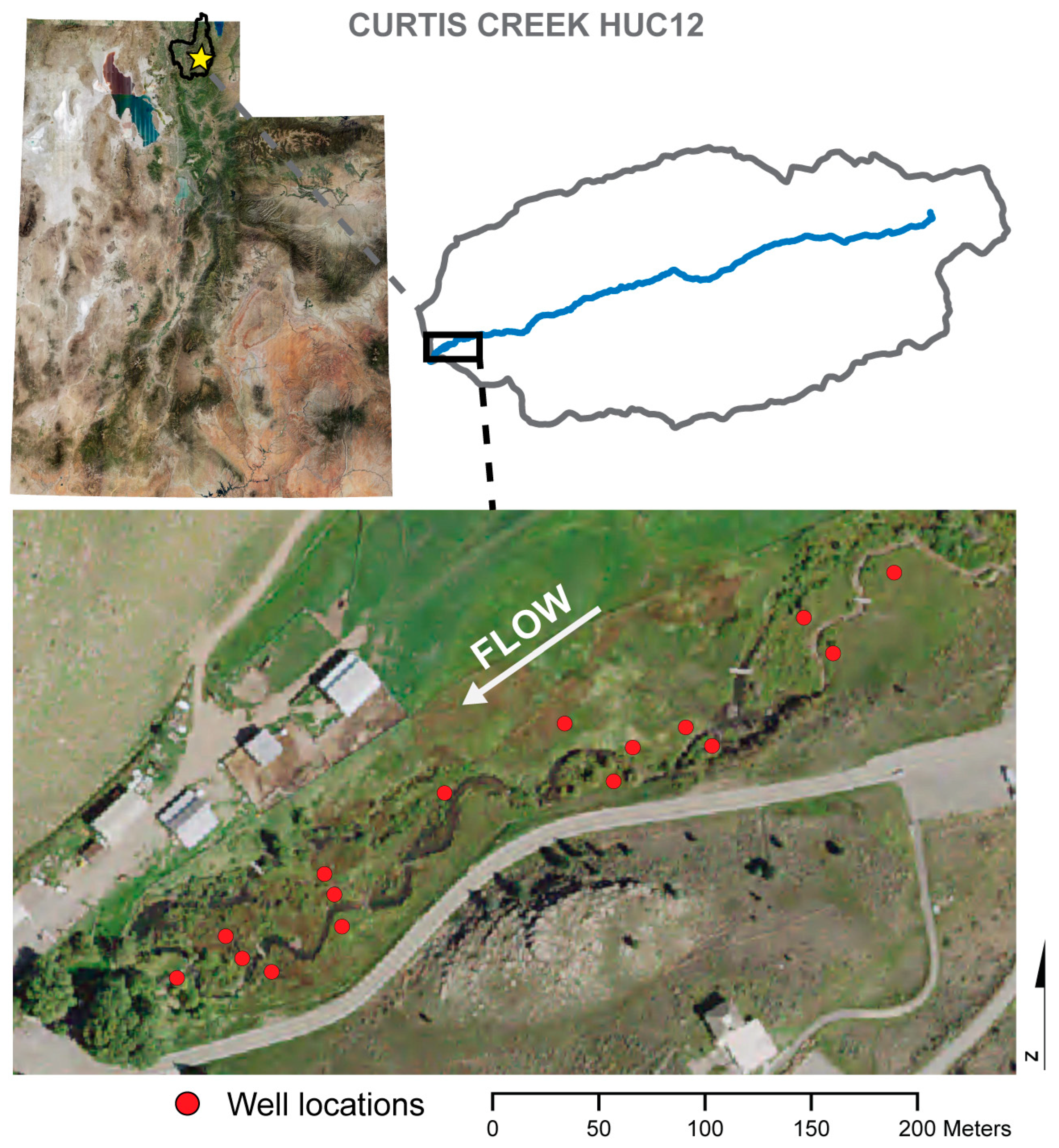
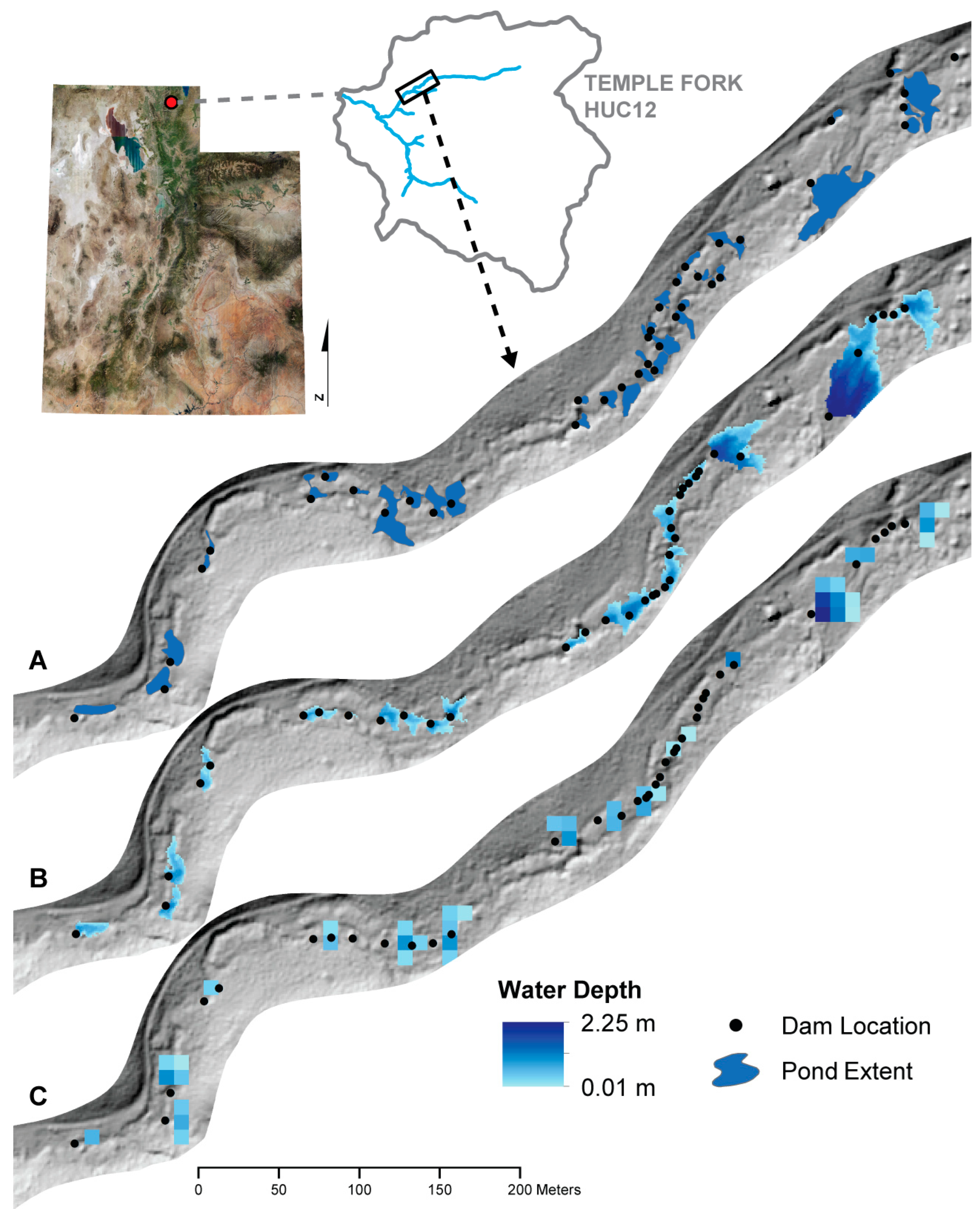
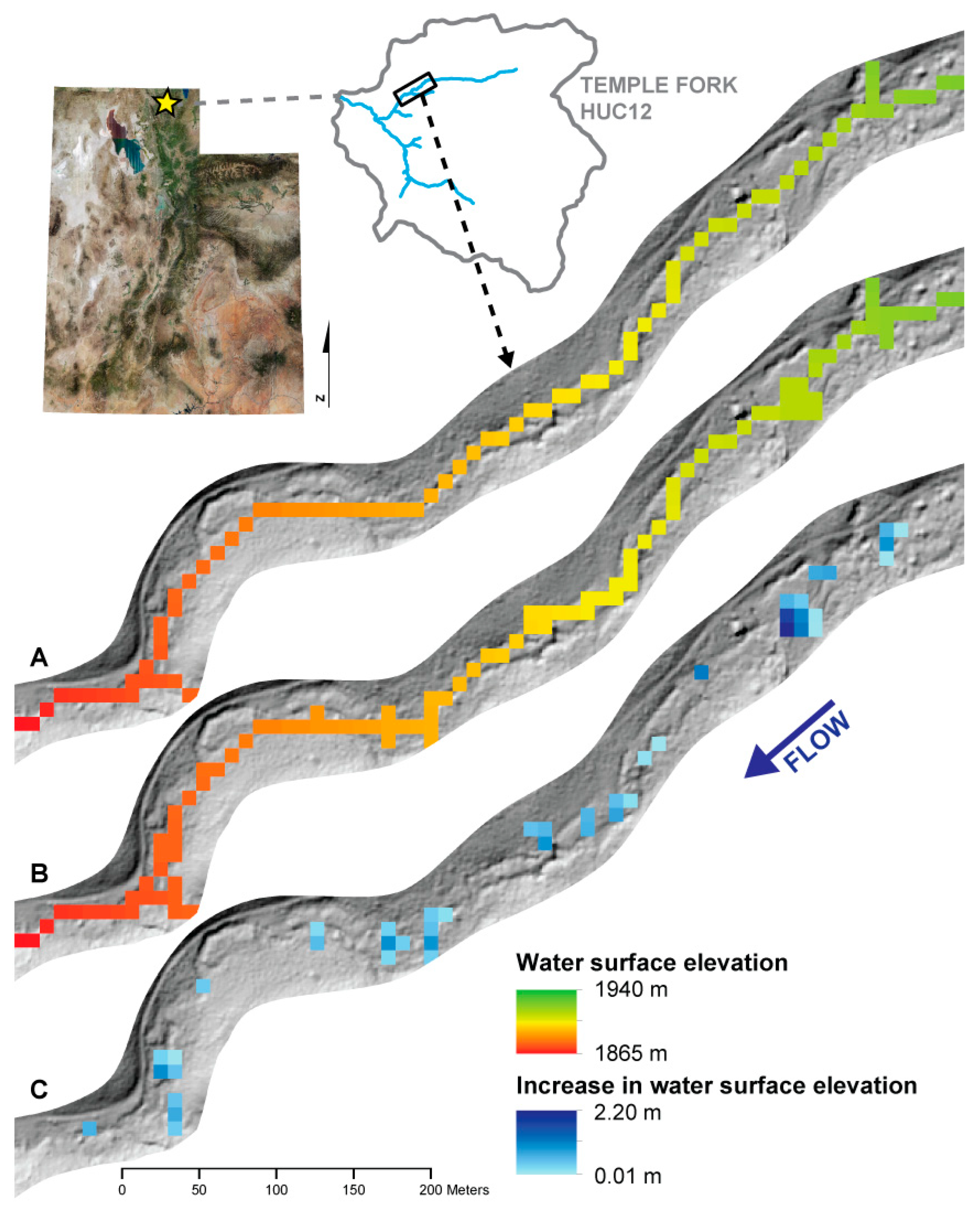
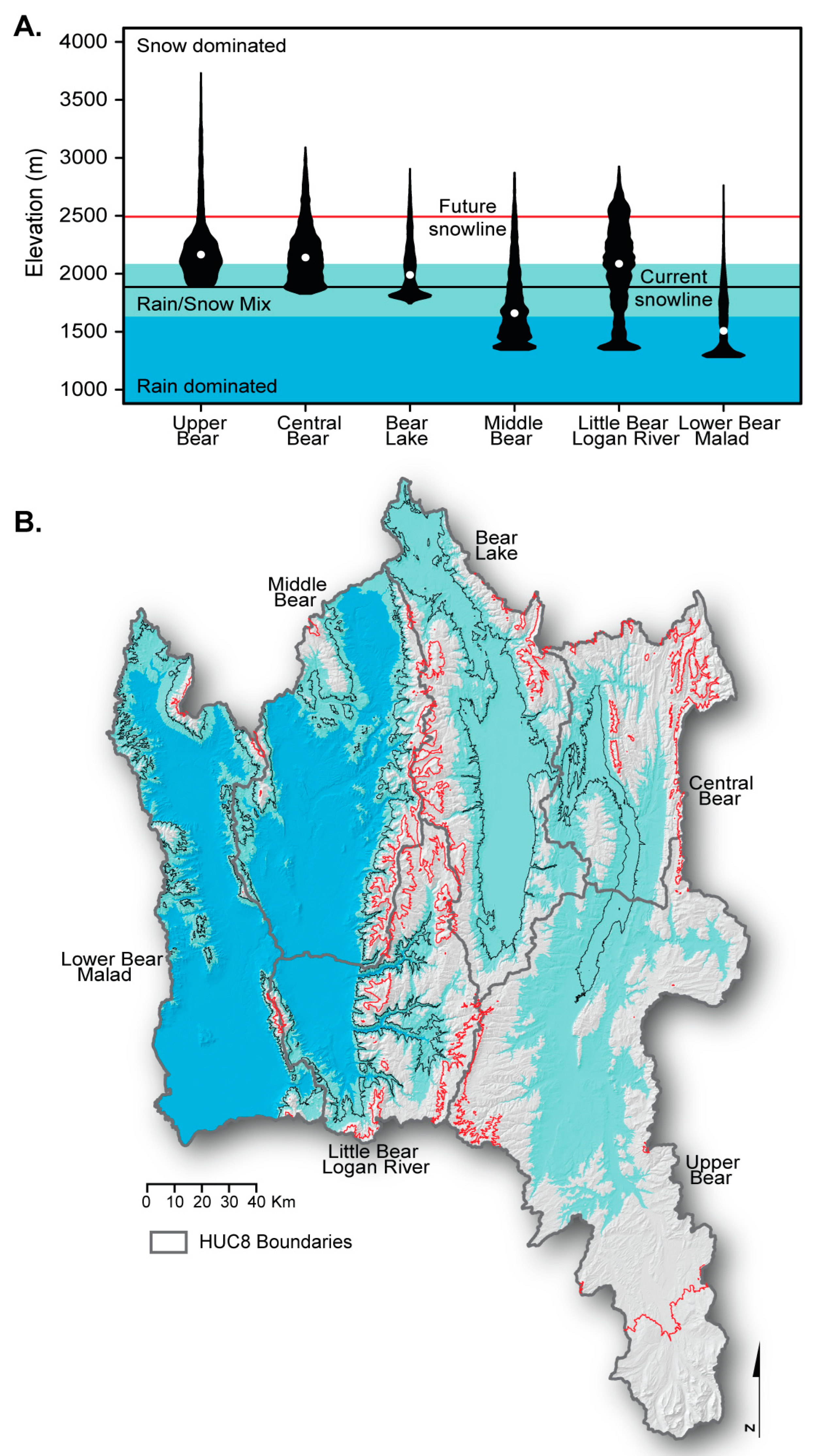
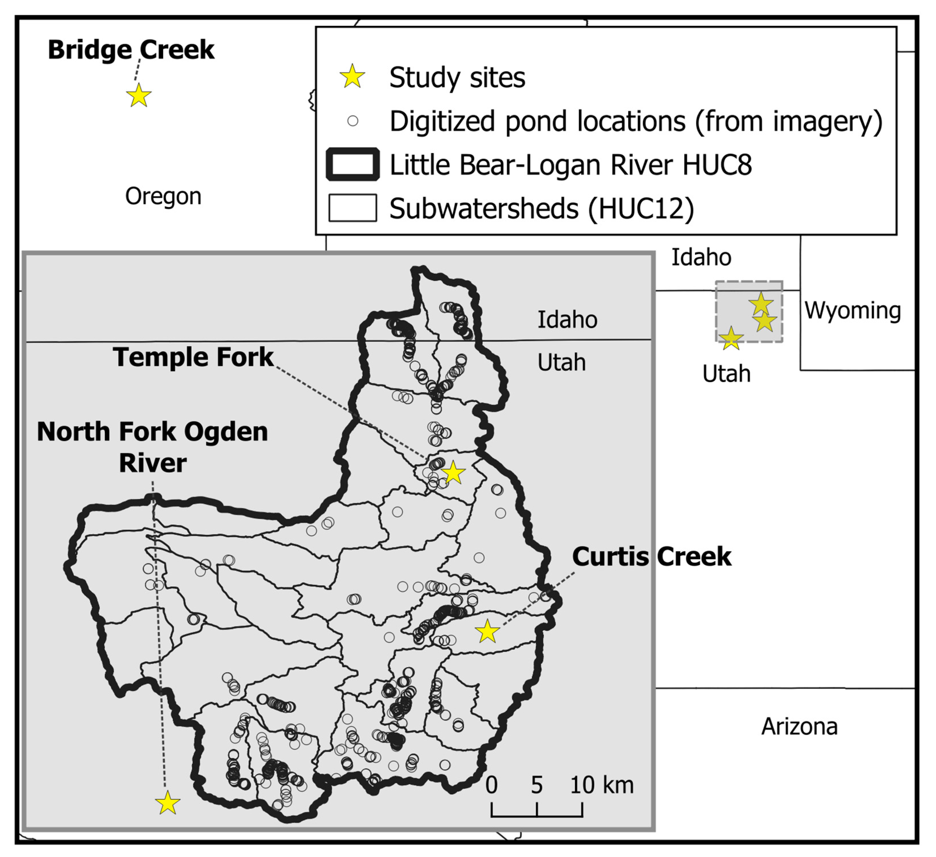
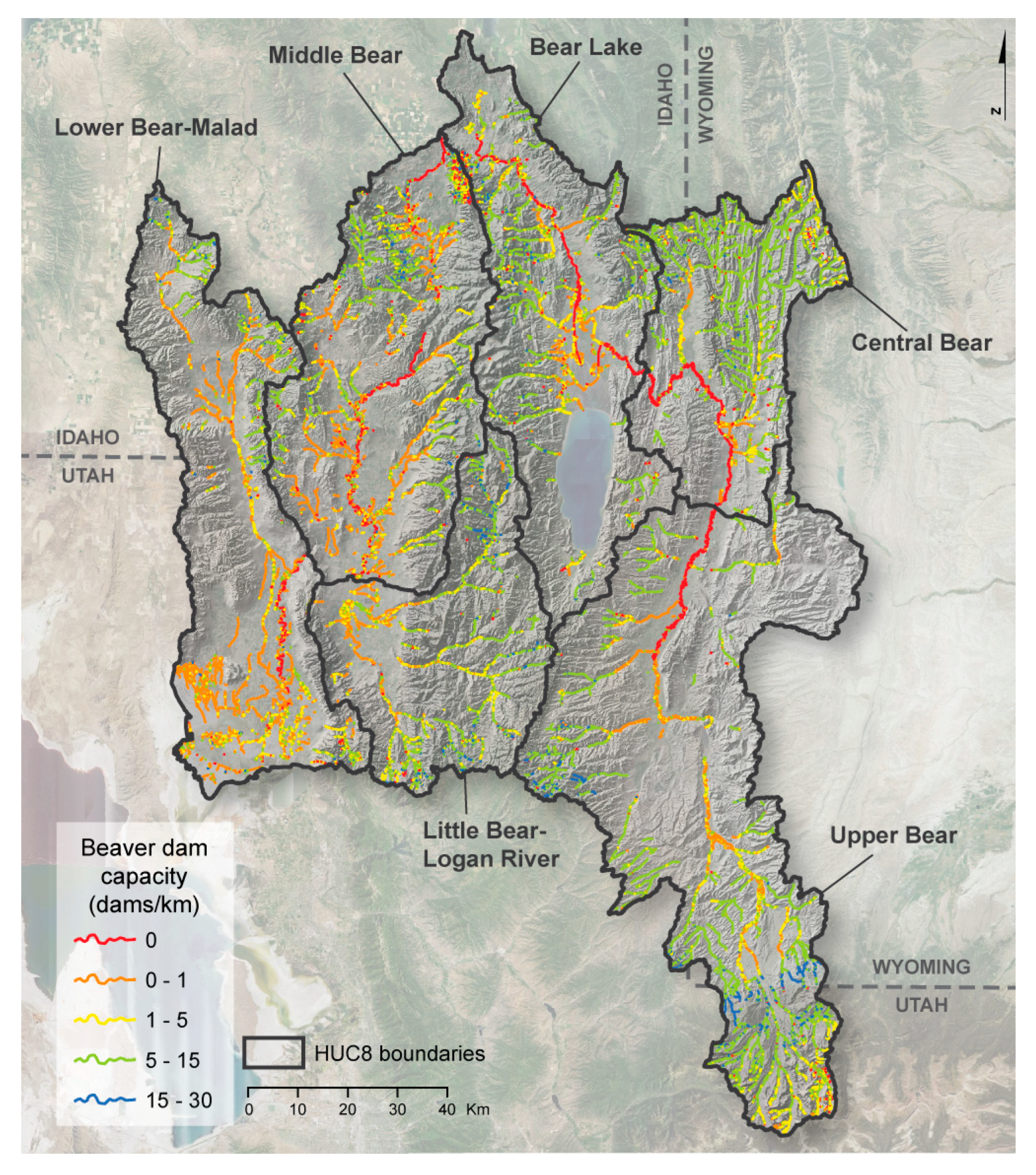
2.1. Study Area

The Bear River basin presents a useful case study because its high relief and aridity are representative of many basins in the western United States where beavers have been extirpated [7]. The mean elevation in the basin is 2000 m and ranges from 1300 m at the Bear River’s outlet to the Great Salt Lake to over 4000 m at its headwaters in the Unita Mountains (Figure 1). The current snowline and treeline elevations are approximately 1900 m and 3300 m, respectively. The Bear River drains 19,450 km² and is divided into six 8-digit hydrologic unit code (HUC8) subbasins and 195 12-digit hydrologic unit code (HUC12) subwatersheds. In the United States, hydrologic unit codes are commonly used to identify standard watershed boundaries, and we use these boundaries herein. Precipitation in the basin ranges from 260 mm in the valleys and uplands to 1400 mm in the snow-dominated alpine zones. The precipitation phase ranges from rain-dominated to a snow–rain mix, and alpine zones are generally snow-dominated (see Appendix A). Overall, approximately 43% of precipitation in the basin falls as snow [27].

From its headwaters in the Unita Mountains of northern Utah (along the Wyoming border), the Bear River flows north through Wyoming, west into Utah, north into Idaho, then takes a U-turn south into Utah, before terminating at the Great Salt Lake (Figure 1). At over 790 km, the Bear River is the longest river in North America that does not drain to an ocean. The Bear River basin contains 6591 km of perennial tributaries and 1664 km of intermittent tributaries.

The combined maximum water storage of the twenty-eight major reservoirs (i.e., dams 15.24 m (50 ft) or more in height, with a normal storage capacity of 6.17 million m³ (5000 acre-feet) or more, or with a maximum storage capacity of 30.83 million m³ (25,000 acre-feet) or more) in the basin is 383.1 million m³ [28]. The State of Utah has explored options for constructing additional reservoirs to store 33.3–271.4 million m³ of water in the Bear River basin to meet anticipated water demand from population growth [29].

Previous studies in the basin have examined the impacts of beaver dams on ecological systems and hydrological regimes [14,30]. Beaver dam abundance throughout parts of the basin has also been quantified [7,20]. Additionally, special conservation regulations and management plans have been implemented to bolster and maintain existing beaver populations [31].

2.2. Modeling Beaver Dam Capacity

Estimates of beaver dam capacity (i.e., the maximum number of beaver dams a stream reach can support) were calculated with the Beaver Restoration Assessment Tool (BRAT) capacity model. This model calculates the maximum dam density (dams/km) for individual stream reaches (~300 m segments). Inputs to the BRAT model include a 10 m digital elevation model (DEM, which was also used to model water storage), land cover information, and regional streamflow equations. We implemented and parameterized BRAT as described in the original publication and refer readers to the BRAT publication for specific details of the dam capacity model [7].

Dam densities from the BRAT capacity model were converted from dams/km to dam counts by dividing by 1000 (m/km) and multiplying by reach length (m), resulting in a maximum number of dams per stream reach. Beaver dam capacity scenarios of 5%, 25%, 50%, and 100% of maximum dam capacity were considered for each HUC12 in the Bear River basin. For example, in a HUC12 where BRAT estimated a capacity of 50 beaver dams, 3, 13, 25, and 50 beaver dams were modeled in the HUC12 under each respective scenario. Modeling multiple dam capacity scenarios accounts for the dynamic nature of beaver dams by giving a range of potential water storage estimates.

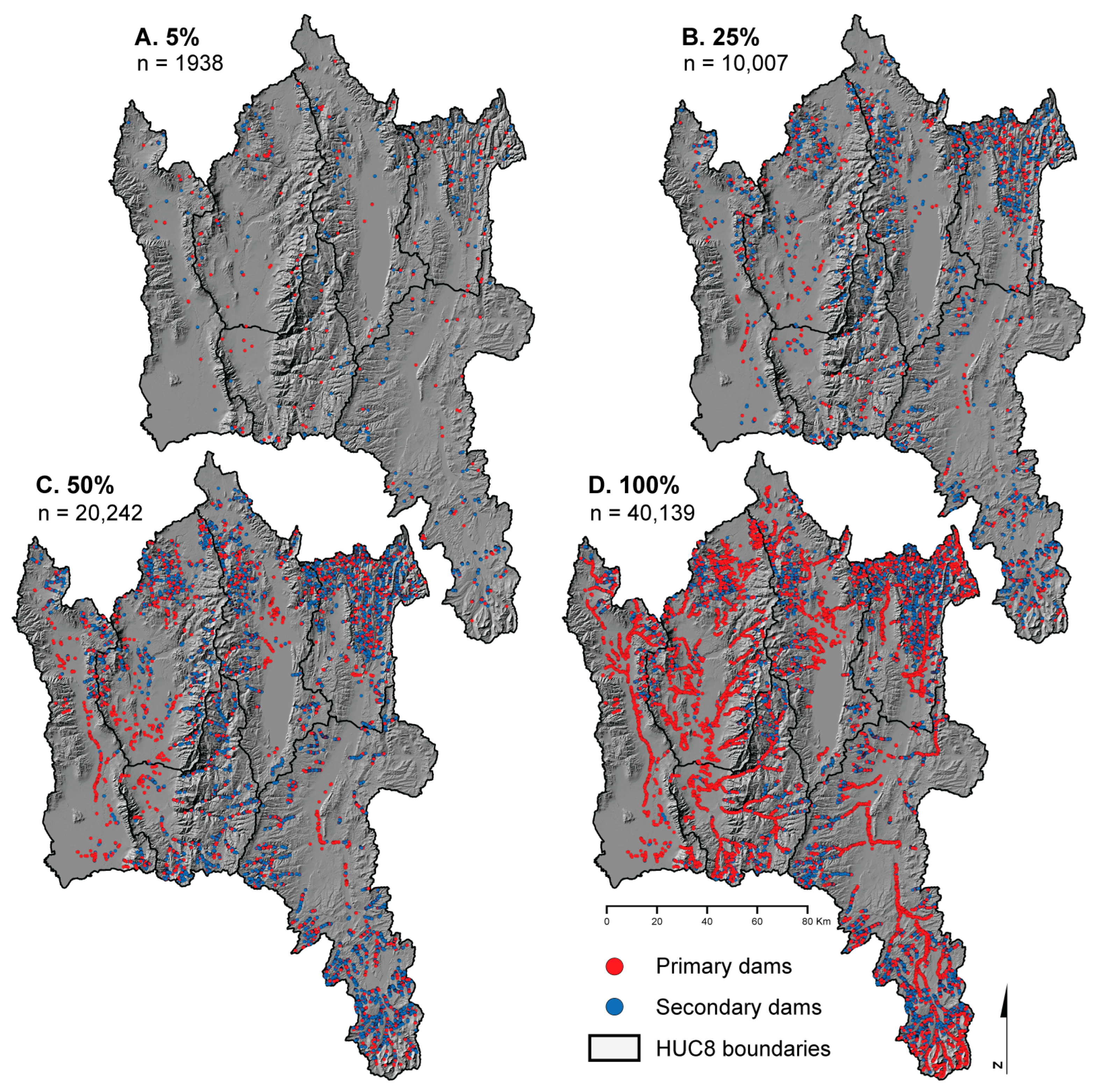
Placement of Individual Beaver Dams

The BRAT capacity model provides spatial estimates of maximum beaver dam density but does not simulate the exact location of individual beaver dams on a stream reach. Dam location simulations were generated for the number of dams estimated by the four different dam capacity scenarios (5, 25, 50, and 100% of dam capacity). The modeled dams in each HUC12 were spatially distributed according to the BRAT dam capacity estimates. Starting with the reaches containing the highest estimated capacity (i.e., the best building habitat), dams were added to the reach until the maximum capacity was reached. Then the stream reach with the second highest estimated dam capacity was filled and so on, until the total number of dams to be modeled was allocated.

Beavers generally construct dams in spatial groups referred to as beaver dam complexes [20]. In the Bear River basin, complexes tend to consist of one primary dam, where a lodge and/or food cache is constructed and secondary dams which provide deep water for protection and to expand the beavers’ foraging range [20]. Starting with the top-ranking 300 m stream reach, a random number of dams were generated from a lognormal distribution with mean 1.55 and variance 0.72, representing the number of dams per dam complex [20]. These dams were spaced evenly along the stream reach, and dams were added to reaches, until the total number of dams specified for each HUC12 capacity scenario was obtained. Each modeled complex contained one primary dam, with all the remaining dams classified as secondary dams.

The differentiation of dam types is important for modeling pond volume, because primary dams are generally larger than secondary dams [20]. For each dam (in a dam complex), the probability of a ‘primary’ classification was one divided by the number of dams in the complex not yet placed on the reach. Once a secondary dam was placed on the reach, the number of dams to be placed in a complex decreased, increasing the probability that the next dam would be classified as primary. Once a primary dam was placed in a complex, all the remaining dams were classified as secondary. If the number of dams selected from the complex size distribution was greater than the maximum estimated capacity of the stream reach, the dam capacity estimate (calculated from BRAT) was used.

After dams were placed along stream reaches, dam locations were shifted to the nearest cell of a rasterized stream network derived from the input DEM. No more than one beaver dam was placed in each 10 m cell. This spacing is consistent with the observed dam spacing and densities.

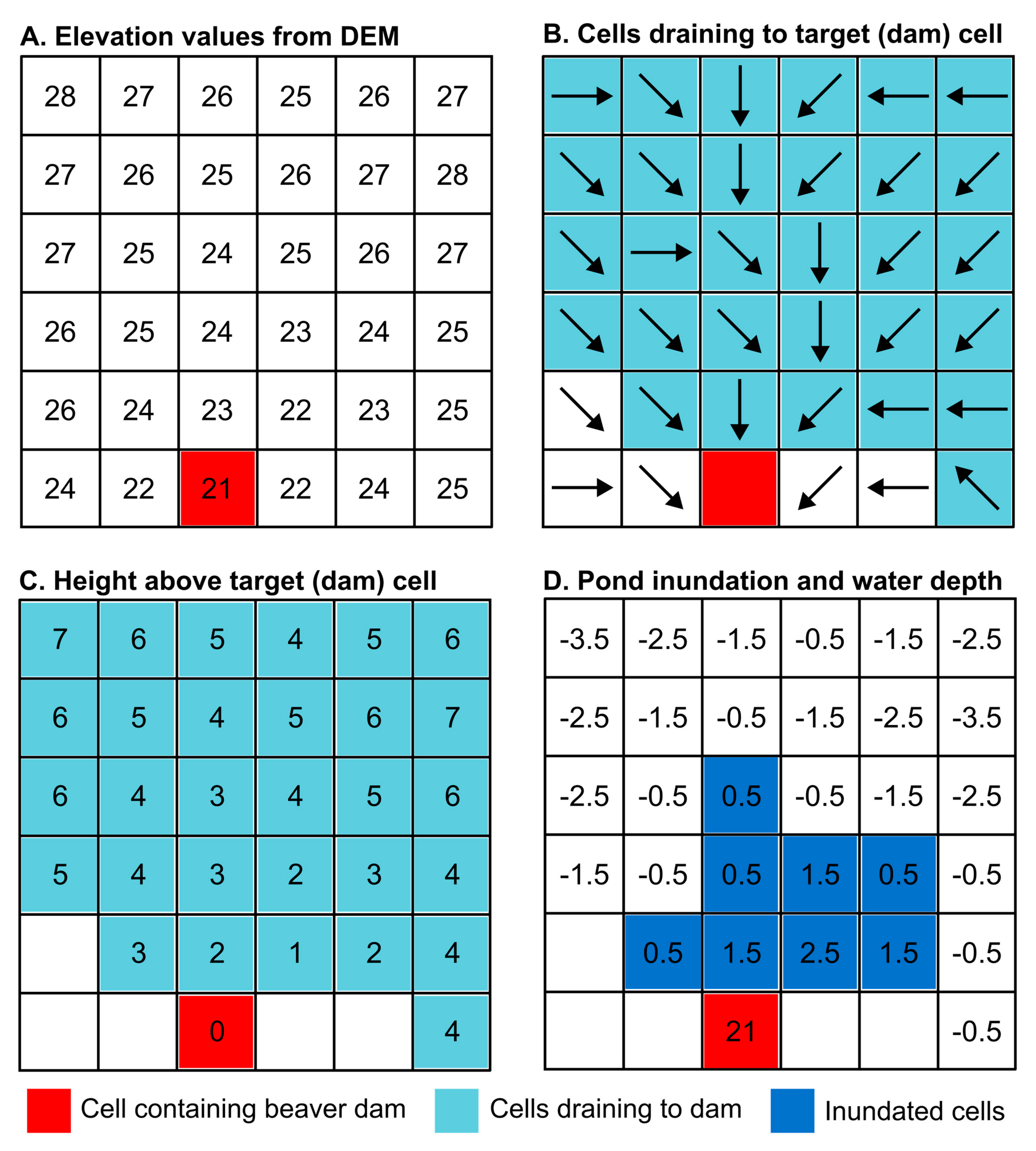
2.3. Modeling Beaver Pond Water Storage

2.3.1. Surface Water Storage Model

We expected the volume of water inundated by a beaver dam and the extent (i.e., area) of inundation to be a function of the height of a beaver dam and the topography inundated.

Based on published dam height information in the Bear River basin and surrounding areas [20], three dam height scenarios were tested for each simulated dam location. The height of primary dams was modeled from a lognormal distribution with mean 1.33 m and variance 0.47 m, and the height of secondary dams from a lognormal distribution with mean 0.87 m and variance 0.31 m [20]. At each dam location, the appropriate dam height distribution (for a primary or secondary dam) was randomly sampled 30 times. One simulation estimated water storage for the median of the sampled distribution, and two additional simulations estimated water storage of the 0.025 and 0.975 quantiles of the sampled distribution. These three scenarios provide the bounds of the extreme water storage values, based on variations in beaver dam height.

We represented topography in our study areas with 10 m DEMs from the USGS National Elevation Dataset (NED), which are available for the entire United States [32]. At the time of this study (2017), the 10 m NED DEMs were the highest-resolution topography products available that covered the entirety of the Bear River basin. Additionally, we leveraged 1 m DEMs that coincided with areas of beaver activity to validate model outputs at the specific study sites of Bridge Creek, Oregon (OR), Curtis Creek, Utah (UT), and Temple Fork, UT. These study sites and modeling methods are described in the sections below.

With the DEMs, we implemented the height above nearest drainage (HAND) algorithm [33] to estimate the areal extent and surface volume of beaver ponds resulting from beaver dam construction. With HAND, the height of a target cell is determined as the elevation of the channel cell to which the target cell drains subtracted from the elevation of the target cell (Figure 2) [33]. Because of HAND’s simplicity, and because it does not require hydrological parameters, it can be applied to moderate-resolution DEMs (e.g., 10–30 m) over large spatial extents [33,34]. HAND has specifically been implemented to estimate inundation extent and water depth for flood mapping as an alternative to cross-sectional 1D hydraulic models (e.g., HEC-RAS) [34], which is similar to our application when a continuous flood stage is substituted for discrete beaver dam heights.

To make a distinction between the original HAND algorithm and the HAND application herein, we refer to our implementation of HAND as HAND for beaver dams, or bHAND. The bHAND methodology was implemented as follows (Figure 2). From a DEM, an eight-direction flow direction raster was created. A cell was selected to represent the location of a beaver dam of a specified height. Using the flow direction raster, all the cells draining to the location of the beaver dam were identified. The height of each cell above the cell containing the dam was calculated as the elevation of the dam cell subtracted from the elevation of the cell draining to the dam. For each cell, the water depth was calculated as the height of a cell above the dam’s location subtracted from the height of the dam. Positive values represent the water depth of the beaver pond, and values less than or equal to zero represent cells that would not be inundated by the dam. This algorithm assumes that the water surface elevation of the modeled pond is equal to the elevation of the beaver dam (i.e., ponds are completely filled to the dam crest).

In equation form, the modeled beaver pond depths could be written as

$$\begin{array}{c}{h}_i^{water}=H_{dam}-H_{DEM i}=\left(H_{target}+h_{dam}\right)-\left(H_{target}+{\Delta h}_{above target i}\right)\\ =h_{dam}-{\Delta h}_{above target i}\end{array}$$

where $H_{dam}$ is the dam crest elevation (above sea level), $H_{DEM i}$ is the DEM elevation value of the cell i (pixel elevation), $H_{target}$ is the elevation value at the foot of the dam, $h_{dam}$ is the height of the beaver dam, and ${\Delta h}_{above target i}$ is the relative level of the cell i in relation to $H_{target}$.

The stream network was represented as all cells with an upstream contributing area greater than 1 km. Dam locations were snapped to this rasterized stream network, and the pond area and volume were modeled with bHAND at the dam locations. The algorithms for this workflow were implemented and automated using the Python programming language with the Geospatial Data Abstraction Library (GDAL). The code is available at https://github.com/konradhafen/beaver-dam-water-storage (accessed on 14 May 2024).

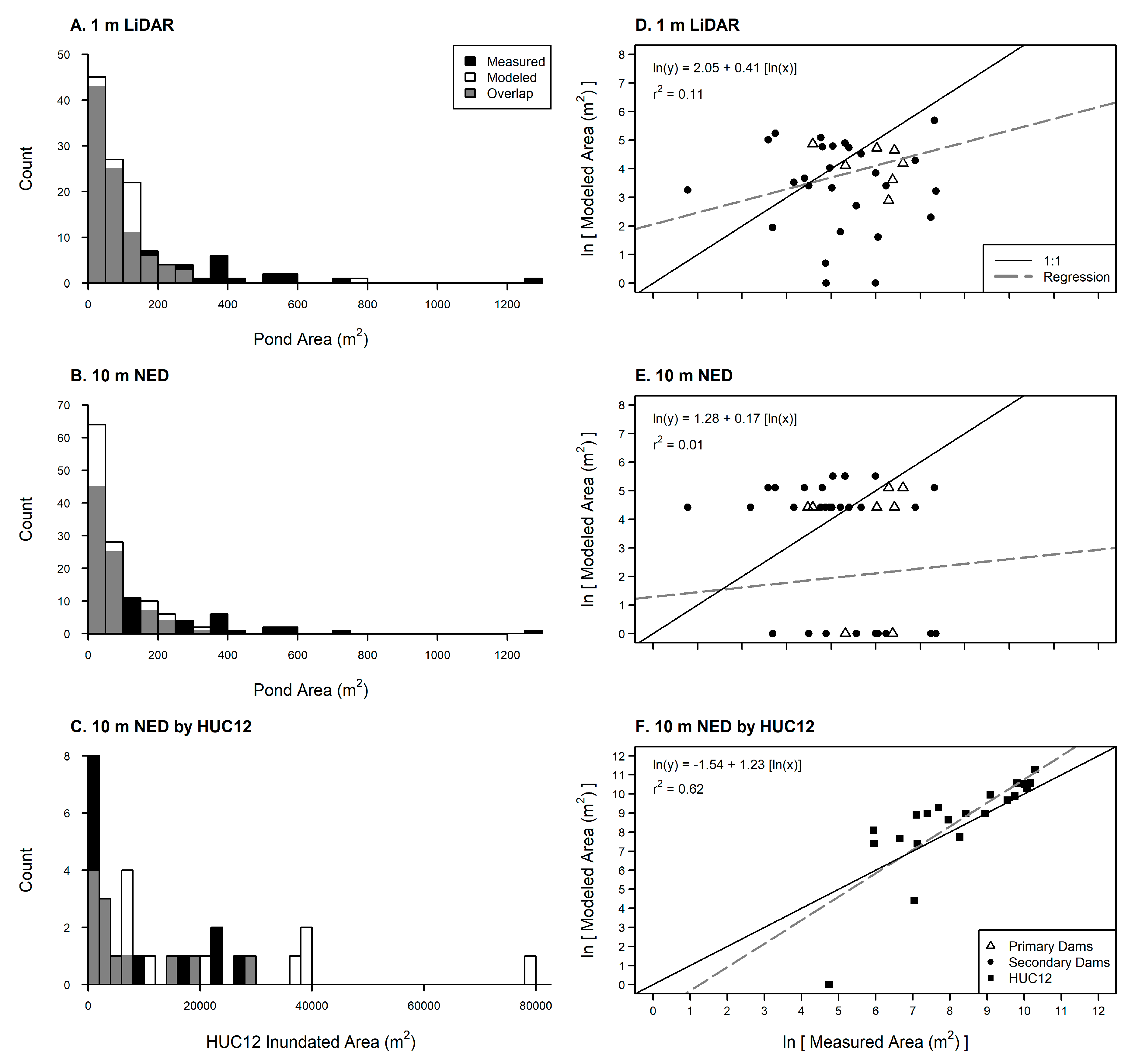
2.3.2. Surface Water Validation Data

The modeling domain for this study was the Bear River basin, as described above (Figure 1). Data from additional study sites that occur both within and outside of the Bear River basin were used to develop and validate the modeling methods (Figure 3;

Table 1. Data used for validation of the surface water estimation model.

Study Site	Data Source	Measured Variables	Count
Bridge Creek, OR	0.1 m bathymetric DEM	Maximum pond volume	32
Curtis Creek, UT	0.1 m bathymetric DEM	Maximum pond volume	8
Temple Fork, UT	0.1 m bathymetric DEM	Maximum pond volume	16
North Fork Ogden River, UT	Field survey	Pond area	34
Temple Fork, UT	Field survey	Pond area	74
Little Bear–Logan River	Aerial imagery	Pond area	1211

).

In the Little Bear–Logan River HUC8 (within the Bear River basin), we identified beaver dam locations and associated beaver ponds from Google Earth imagery (Figure 3). Dam locations were digitized as points, and pond areas were digitized at polygons. The pond areas were used to validate the bHAND outputs.

Field surveys that measured the height of dams and the area of beaver ponds were conducted in the Temple Fork and North Fork Ogden River subwatersheds (Figure 3). The methodology for measuring the beaver dam heights and the resulting data were previously published [20]. In addition to the published data, the beaver pond area for associated beaver dams was measured by walking the perimeter of each beaver pond, while tracking movement with an iPad containing GPS and GIS functionality [20]. Thus, we obtained the dam height for a pond and the associated pond area.

Digital elevation models (DEMs) from high-resolution topographic surveys of river bathymetry at Bridge Creek, OR and Curtis Creek, UT (Figure 3), were used to identify beaver dam heights, associated beaver pond areas, and associated beaver pond volumes. When a dam was identified in the DEM its location was marked and its height determined as the difference between the maximum elevation of the dam crest and the minimum elevation in the stream channel at the dam base. The maximum upstream area expected to be inundated by the dam was digitized as a polygon. Within the maximum inundation area, the water depth was calculated for pixels lower than the maximum dam crest elevation as the pixel’s elevation subtracted from the dam elevation. Pond areas were calculated as the count of inundated pixels multiplied by the DEM’s pixel area. Pond volumes were calculated as the sum of water depths multiplied by the DEM’s pixel area.

2.3.3. Surface Water Storage Validation

Three separate datasets of observed beaver pond area and volume were used to validate the bHAND results (Table 1).

We compared pond areas modeled with bHAND to surveyed pond areas from field assessments at the North Fork Ogden River and Temple Fork sites. At the location of each field-surveyed beaver dam where a pond area was recorded, we used the measured dam height to model the resulting beaver pond with bHAND. We conducted these simulations with both 1 m and 10 m DEMs. We assessed the results with a linear hypothesis test, to simultaneously determine if the intercept and the slope of the regression line between the modeled and observed data differed from zero and one, respectively. We also fitted a regression with an intercept of zero, and with Student’s t-test determined if the slope of the modeled regression line was significantly different than one. We performed both statistical analyses to provide transparency in the model validation. We included the t-test because, while forcing an intercept of zero makes physical sense for validation, however, the coefficient of determination (r²) for the resulting regression model does not accurately represent the amount of variation explained by the model.

We also tested the performance of bHAND, using 10 m DEMs to estimate the pond area at the 1211 dam locations digitized from aerial imagery in the Little Bear–Logan River watershed. It was not possible to collect dam heights from aerial imagery; therefore, we did not link dam heights to pond areas for this analysis. For these simulations, the dam type (primary or secondary) was randomly determined from the frequency of field observations (15% primary dams, 85% secondary dams) [20]. Dam heights were estimated as a function of dam type (primary or secondary) and discharge (obtained for each stream reach from BRAT outputs) from equations generated for the area from survey data [20]. We summed the digitized and modeled pond areas for each HUC12 in the Little Bear–Logan River watershed and validated the modeled and digitized beaver pond areas based on the total inundated area in a HUC12. This aggregated validation approach was used because individual dam heights were not available.

From high-resolution topographic surveys which included beaver dams and ponds at Bridge Creek, OR, and Temple Fork, UT, we determined the heights of beaver dams and the volumes of beaver ponds (as described in Section 2.3.2). Using bHAND, the beaver pond volume was modeled at surveyed dam locations with the surveyed height of each dam. We tested for deviations between the modeled and observed (from field surveys) pond volumes with a linear hypothesis test and Student’s t-test, as described above.

The described methods present three different validation tests for the bHAND-modeled estimates of beaver pond area and volume. In the first method, the dam height and pond area were obtained from field surveys, allowing us to validate the proficiency of bHAND in replicating observed pond areas, given the dam height. In the second method, the total inundated area within a HUC12 was known, but specific dam heights were not. These data allowed us to validate how well the modeled distributions of primary and secondary dams and their associated heights replicated the inundation extent at the subwatershed (HUC12) scale. The third method provided data to assess how accurately bHAND replicated observed pond volumes.

2.3.4. Groundwater Storage Model

Changes to groundwater elevation resulting from the construction of beaver dams were modeled only within valley bottoms (i.e., the stream channel and adjacent floodplain [35]) adjacent to perennial streams for which the beaver dam capacity was estimated. Valley bottom extents were delineated using the Valley Bottom Extraction Tool (V-BET), which implements variable slope thresholds based on drainage area to identify valley bottom extents [36]. The V-BET outputs were visually validated and edited to resolve any inconsistencies. This limited the modeling domain to areas where beaver dams have the greatest potential to influence groundwater. In general, valley bottom widths ranged from 10 m in confined headwater reaches to 2500 m in the unconfined valley of the Bear River.

We assumed that beaver dams persisted long enough for adjacent soils to become fully saturated and that the water supply was sufficient to maintain the pond surface water elevation and soil saturation throughout the duration of the year. The purpose of groundwater modeling was not to address groundwater dynamics, but rather to identify the potential maximum water table if the modeled ponds were filled to the dam crest year-round and the water table elevations were not limited by ET or the rate of infiltration from the stream or pond to the groundwater. Modeling was limited to the valley bottoms of perennial streams, because they represent these assumptions more closely than intermittent streams, where beaver dams may be completely dry by late summer (as personally observed in our study area). We used MODFLOW-2005 [37,38], a three-dimensional third-order finite groundwater model developed by the USGS, with equations for saturated flow, to model water table elevations representing conditions with and without beaver dams in the study area’s valley bottoms.

The valley bottom aquifer was modeled as a single layer, with the bottom boundary of the model extent set 10 m below the land surface. In Wyoming, near the Utah border, the depth of aquifers adjacent to the Bear River and its tributaries range from 5 m along some tributaries to greater than 137 m in the Bear River valley [39,40]. Because data describing aquifer depths throughout the Bear River basin were unavailable, we modeled all aquifers with a depth of 10 m as a compromise between deep aquifers in wider, alluvial valleys and shallower, headwater aquifers. The MODFLOW grid was of the same extent and resolution (10 m) as the input DEM for the BRAT and bHAND models. This DEM was used as the upper model domain boundary (i.e., the surface elevation of the valley bottom).

MODFLOW was parametrized with mean horizontal and vertical hydraulic conductivity (K) values for soils in each HUC12. Estimates of K were obtained through area and depth-weighted averages from the US Department of Agriculture (USDA) Soil Survey Geographic (SSURGO) database [41]. In each HUC12, we applied a single value for both the vertical and horizonal K by averaging the SSURGO values in the HUC12 valley bottoms. In instances where no soil data were available within a HUC12, the mean K values for the larger HUC8 were used. HUC12 averages for horizontal and vertical K ranged from 0.67 to 161.10 µm/s and from 0.60 to 60.43 µm/s, respectively.

Four steady-state MODFLOW simulations were run for each HUC12, to represent the water table elevation with no beaver dams and the water table with beaver dams modeled with low (0.025 quantile), median, and high (0.975 quantile) dam heights. The first simulation represented conditions with no beaver dams. This was accomplished by setting constant head boundaries along a rasterized stream network, with the hydraulic head value equal to the stream elevation (i.e., the water surface elevation was estimated to equal the elevation along the stream from the 10 m DEM) at all points along the rasterized network. For the other three simulations, which represented the dam height scenarios, the constant head boundaries were adjusted to include areas predicted to be inundated by bHAND. The hydraulic head at these locations was set to the elevation of the modeled beaver pond, and the upper model domain extent was adjusted to reflect these changes (see Appendix A). The lower model domain was not adjusted. No-flux boundaries were defined along the edges of the model domain (i.e., the bottom and sides of the valley bottom).

This parameterization assumes the full depth of the soil mantle adjacent to all streams can serve as an aquifer, the lower model domain is impermeable, fill throughout the aquifer is homogeneous, there is no groundwater drawdown or ET, and groundwater is derived from streams, with no groundwater contribution from hillslopes. Additionally, geomorphic changes resulting from beaver activity (e.g., beaver-dug channels) or beaver dams (e.g., the aggradation of sediment and organic matter, excavation of material from beaver ponds, or creation of overflow channels) are not represented. This is a simplified implementation of MODFLOW that is designed to identify the maximum potential groundwater storage from beaver dams over a diverse area with little data for model validation.

The change in water table elevation resulting from beaver dam construction was calculated as the modeled baseline water table elevation subtracted from the modeled water table elevation after beaver dam construction for each of the three dam height scenarios (low, median, and high). Changes in water table elevation were converted to volumes as the product of water table elevation change, porosity, and model grid resolution. The potential groundwater yield was calculated as the product of water table change and the specific yield (porosity minus field capacity). Unless otherwise stated, groundwater results are presented as potential groundwater yield (porosity minus field capacity). This modeling approach allowed us to quantify net changes in groundwater storage over several large HUC8 sub-basins. To improve the model results and reduce computational run times, we divided the study area by HUC12s and ran each HUC12 through the groundwater-modeling process individually using the FloPy Python module [42].

2.3.5. Groundwater Storage Validation

The modeled change in groundwater depth was evaluated against observations from groundwater wells in a stream reach before and after beaver dam construction. Observed data were obtained from a previous study at Curtis Creek, UT (Figure 3) where groundwater wells were installed in 2008, after which beavers constructed many dams in the same reach between 2009 and 2012. From 2008 to 2012, the groundwater elevation was measured at each well with a depth sounder at least twice per year between the months of April and October.

A detailed topographic survey of the study site in 2012 recorded the location and size of beaver dams and beaver ponds. As with the methods above, we used the topographic survey to identify beaver dam locations and beaver dam heights, then modeled the changes in surface and groundwater storage resulting from beaver dam construction with bHAND and MODFLOW (as described above). The modeled changes in groundwater elevation were compared to the observed groundwater changes (2008–2012) with a linear regression model and linear hypothesis test (as described above).

Because the Curtis Creek study site represents only a small portion of the study area, our validation goal was not to develop an idea model for Curtis Creek. Rather, our goal was to confirm that our simplified implementation of MODFLOW captured the general trend of observed groundwater elevation changes resulting from beaver dam construction.

2.3.6. Estimating Total Water Storage

The total water storage was determined as the sum of the estimated surface water storage and potential groundwater yield. The groundwater yield was calculated as the modeled increase in groundwater level multiplied by the difference in porosity and field capacity. This excluded soil particles, and water that could be held in the soil by capillary forces, from the storage calculations.

We summed the estimated water storage increases from beaver dam construction for each dam height and dam capacity scenario across each HUC12 subwatershed, each HUC8 sub-basin, and for the entire Bear River basin. We also summed the estimated water storage increases upstream of each stream reach. The estimated increase in water storage upstream of each stream reach was then divided by the estimated volume of average August and September streamflow and is presented as a percentage for each stream reach. Monthly streamflow estimates for August and September were obtained for each stream segment via the NHD Enhanced Unit Runoff Method (EROM), which is published as part of the NHDPlus dataset [43]. A common goal of beaver-based restoration activities is to increase late-season water availability [12]. While increased upstream water storage does not represent potential changes to streamflow, it does place an upper bound on the maximum streamflow change that could be expected. This upper bound is useful for evaluating if, and where, desired outcomes from beaver dam construction are plausible.

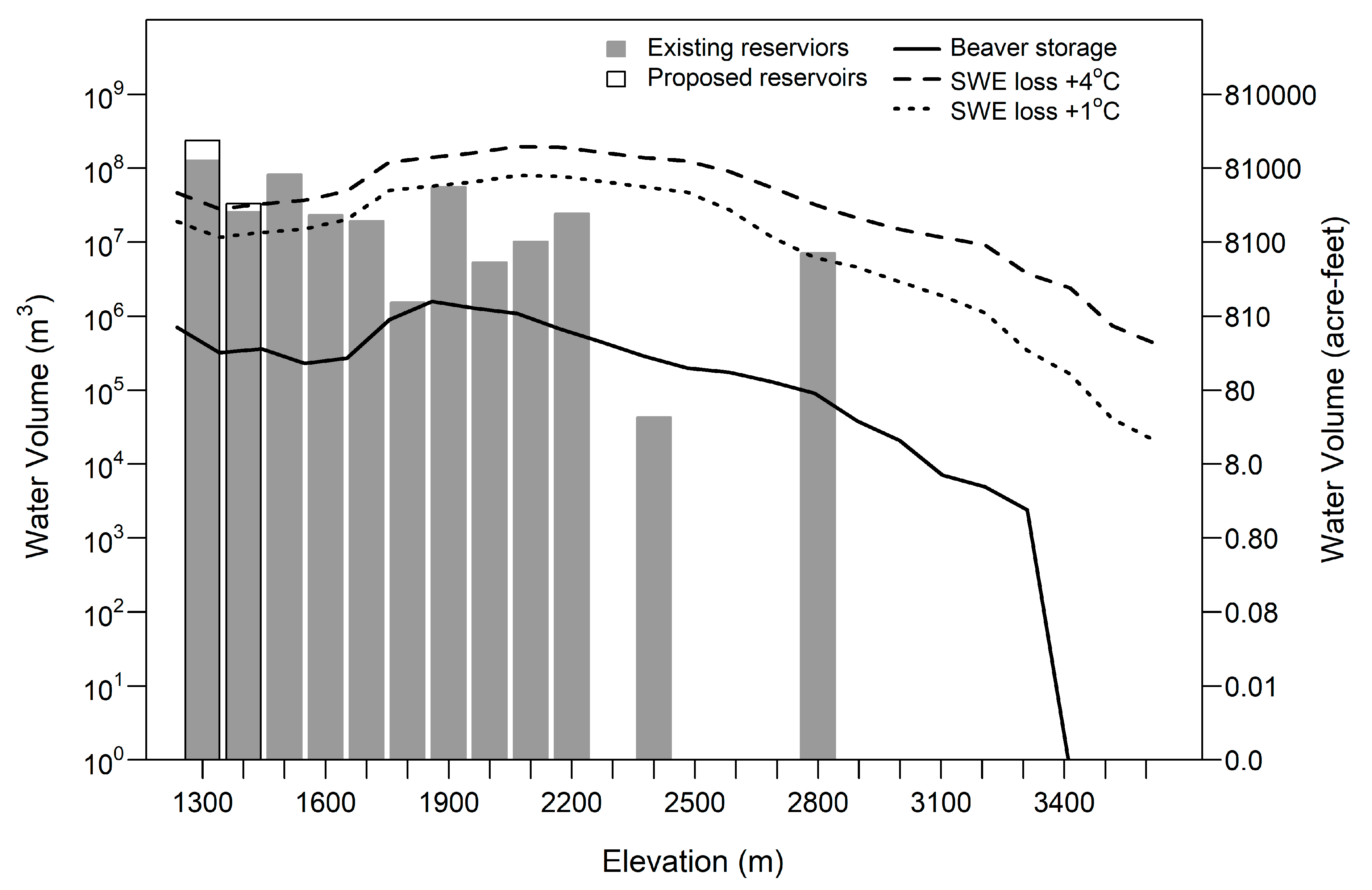
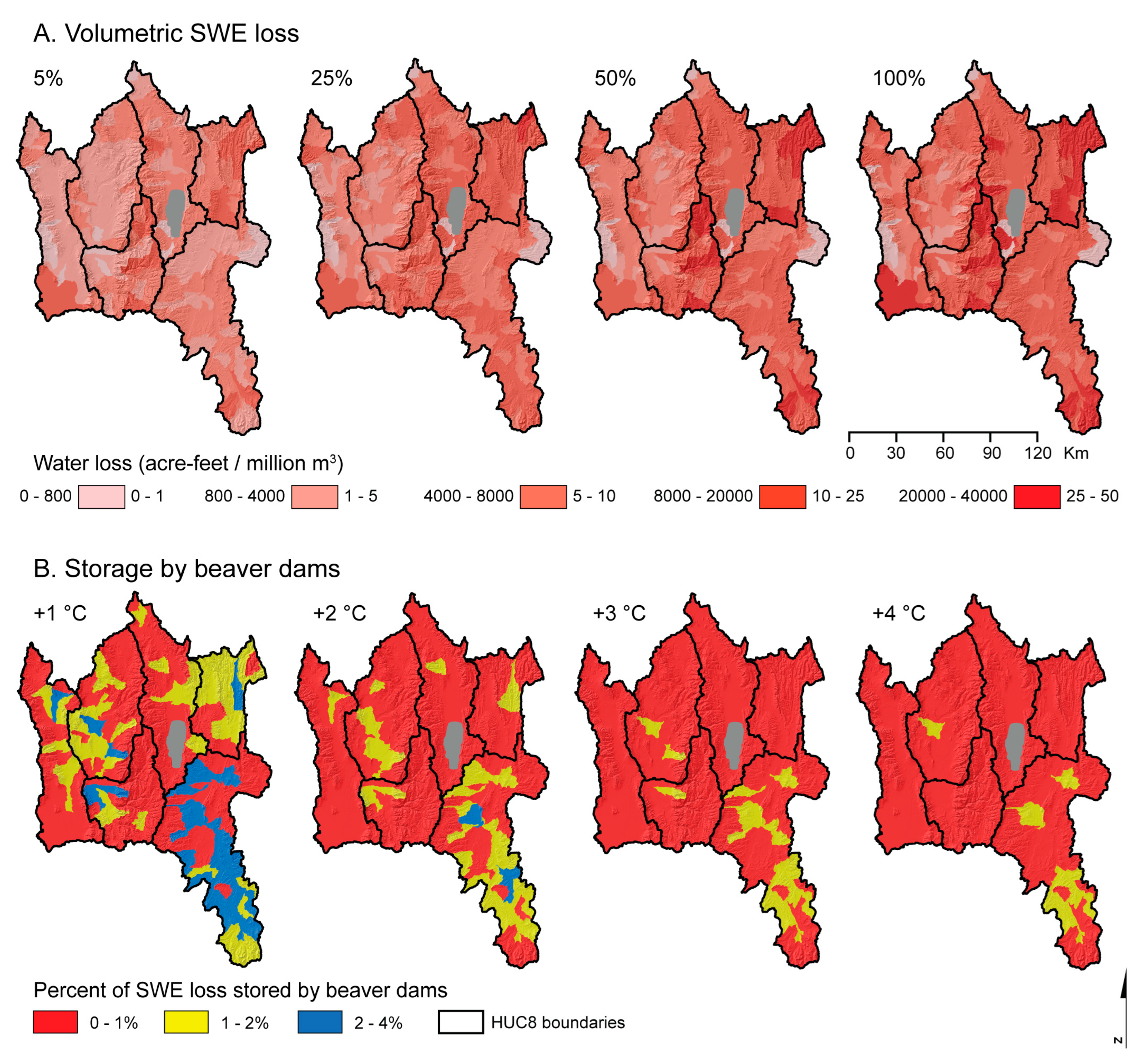
2.4. Estimating Snowpack Decline

To estimate potential snowpack decreases related to warming temperatures, we developed a relationship between elevation and the average annual peak SWE and adjusted this relationship to simulate climate-warming scenarios for +1 °C to +4 °C following the methods of Tennant et al. [44]. We evaluated the average annual relationship between elevation and SWE for the 2004–2015 water years, using data from the National Weather Service spatially gridded (1 km resolution) Snow Data Assimilation System (SNODAS) model [27]. The relationship between elevation and mean SWE (as estimated by SNODAS) was modeled with Richard’s growth function.

$$SWE\left({elev}_i\right)={A\left[1+v exp\left\{1+v+\frac{M}{A}{\left(1+v\right)}^{1+\frac{1}{v}}\left(\mathsf{\lambda }-{elev}_i\right)\right\}\right]}^{-1/v}$$

Three of the four fitted parameters of Richard’s growth function can meaningfully describe measured variables related to SWE at a given elevation SWE(elev_i). λ describes snowline elevation, A maximum SWE (mm), and M the maximum slope of the relationship. v is unitless and influences the shape of the function [44].

Temperature warming was simulated, by applying a moist adiabatic lapse rate of −0.65 °C per 100 m to shift the snowline elevation λ upward under each warming scenario. No other parameters of Richard’s equation were manipulated to simulate warming scenarios. The estimated decrease in the mean maximum SWE for each raster cell was calculated as the estimated mean maximum SWE under a future warming scenario subtracted from the initial estimated mean maximum SWE (i.e., the current condition).

Because the parametrization of Richard’s equation can vary regionally, we qualitatively examined the SWE–elevation relationship in the three primary mountain ranges of the Bear River basin (the Bear River, Wyoming, and Uinta ranges; Figure 1). Differences were observed in the SWE–elevation relationship between the Unita range and the combination of the Bear River and Wyoming ranges. Thus, we developed two fits for Richard’s equation: one for the Unita range and another for the Bear River and Wyoming ranges (see Appendix A).

3. Results

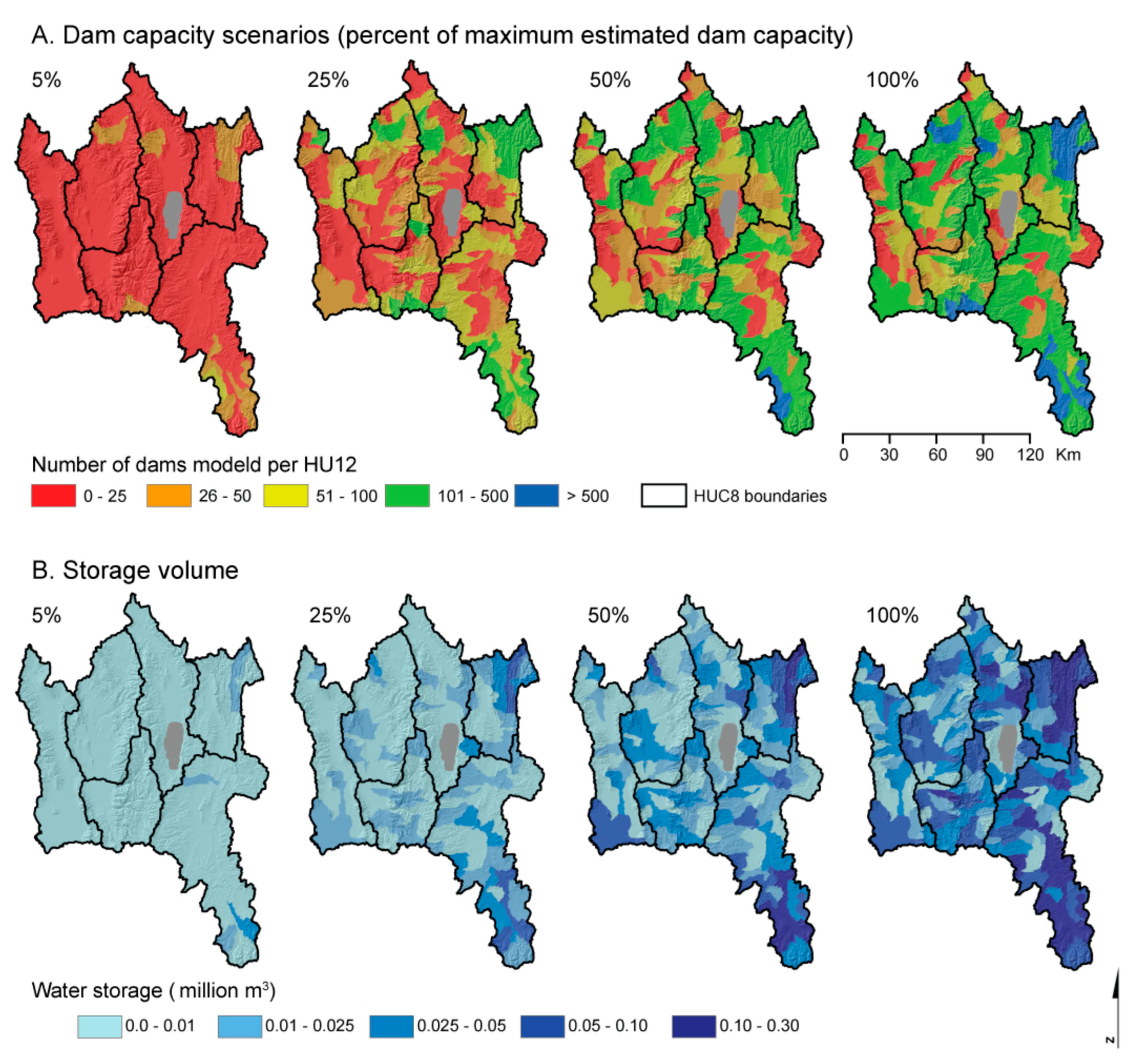
3.1. Beaver Dam Capacity

The BRAT capacity model estimated a maximum capacity of 41,848 beaver dams for the 6591 km of perennial streams in the Bear River basin, resulting in an overall maximum dam density of 6.3 dams/km (Figure 4). For scenarios with beaver dams modeled at 5%, 25%, 50%, and 100% of estimated capacity 1938, 10,007, 20,242, and 40,139 individual dams were modeled, representing 4.6%, 23.9%, 48.4%, and 95.9% of the estimated dam capacity, respectively (Figure 5). Slight differences in the target dam capacity and actual modeled dam capacity arise from converting dam capacity estimates (dams/km) to counts of dams per stream reach. The valley bottoms of perennial streams in the Bear River basin ranged from 3.7% to 12.4% of the total drainage area for individual HUC8s, comprising 7.9% of the entire Bear River basin.

3.2. Beaver Pond Water Storage

3.2.1. Surface Water Storage

Estimates of pond area from bHAND were validated against 74 field-surveyed pond areas from Temple Fork and 34 pond areas from North Fork Ogden River (n = 108). When pond volumes were modeled (with bHAND) using a 1 m lidar input DEM, the intercept (2.05) and slope (0.41) of the regression line between the modeled and observed pond areas differed significantly from zero and one (p < 0.0001). The slope of the relationship also differed significantly from one (0.85; p < 0.0001) when the intercept was held at zero. This indicates that bHAND underestimated the pond areas (Figure 6).

Similarly, when the same analyses were applied to pond areas modeled with bHAND using a 10 m input DEM, the intercept (1.28) and slope (0.17) of the regression line between the observed and modeled pond areas were significantly different from zero and one (p < 0.0001). The slope of the relationship between the modeled and observed area also differed significantly from one (0.45; p < 0.0001) when the intercept was held at zero—again, suggesting bHAND underestimates the pond area with a 10 m DEM input (Figure 6).

When comparing the total area inundated by beaver ponds in a HUC12 (as determined from aerial imagery) to the total inundated area modeled by bHAND in a HUC12 (based on dam height and dam type distributions), the intercept (−1.54) and slope (1.23) of the regression line between the modeled and observed data points (n = 21) did not differ significantly from zero and one (p = 0.2155). With the intercept held at zero, the slope estimate of 1.09 was also not significantly different than one (p = 0.9990). These results indicate that, while bHAND may underestimate the inundation area of individual beaver ponds, the methods used herein to estimate dam height and inundation area produce patterns similar to what is observed at the subwatershed scale (Figure 6).

Comparing the bHAND estimates of the maximum beaver pond volume to pond volumes estimated from high-resolution topographic surveys at Bridge Creek, Curtis Creek, and Temple Fork yielded the following results. When the pond volume was modeled with bHAND, using a 1 m input DEM, the intercept (0.21) and slope (0.97) of the regression line between the modeled and observed pond volumes were not significantly different than zero and one (p = 0.7951). When using a 10 m input DEM to model pond volume with bHAND, the intercept (1.19) and slope (0.67) of the regression line between the modeled and observed pond volumes were not significantly different than zero and one (p = 0.3094). Regressions between the modeled and observed pond volumes indicated that bHAND accounted for 43% and 16% of the variation in pond volume, when 1 m and 10 m DEMs were used as the respective inputs (Figure 7).

3.2.2. Groundwater Storage

The comparison of the MODFLOW-estimated groundwater elevation changes and observed groundwater elevation changes at Curtis Creek over the period from August 2008 to September 2012 produced a linear relationship, with an intercept of 0.17 and a slope of 0.66. The modeled groundwater elevation changes explained 42% of the observed groundwater elevation change (Figure 8). The root mean square error (RMSE) between land surface elevations surveyed at groundwater wells with a real-time kinematic global positioning system (RTK-GPS) and elevations from the 10 m DEM used as the model input was 0.96 m. The RMSE between the observed and modeled groundwater elevation at baseflow without beaver dams on 22 August 2008 (1.11 m) and baseflow with beaver dams on 25 September 2012 (1.05 m) was only slightly higher than the (0.96 m) RMSE of land surface elevations. The RMSE between the observed and modeled changes in groundwater elevation was 0.24 m. Thus, the RMSE values for the water table elevations were comparable to the RMSE inherent between the DEM and land surface elevations.

3.2.3. Total Water Storage

Total estimated increases in transient water storage resulting from beaver dam construction in the Bear River basin ranged from 0.36 million m³ for the 5% dam capacity scenario with median dam heights, to 10.38 million m³ at 100% dam capacity with median dam heights (

Table 2. Number of modeled primary (P. Dams) and secondary (S. Dams) beaver dams, total length of perennial streams (Stream Length), modeled dam density, total change in water storage (TS), change in surface water storage (SWS), and change in groundwater storage (GWS) at median dam height in each HUC8 watershed for each BRAT dam capacity scenario. Values for TS, SWS, and GWS are million cubic meters.

HUC8	BRAT Capacity (%)	P. Dams	S. Dams	Stream Length (km)	Dam Density (Dams/ km)	TS (mil. m3)	SWS (mil. m3)	GWS (mil. m3)
Upper Bear	5	166	412	1605	0.4	0.15	0.04	0.11
	25	880	2261	1605	2.0	0.76	0.24	0.53
	50	1923	4447	1605	4.0	1.73	0.51	1.22
	100	4825	8013	1605	8.0	4.14	1.07	3.07
Central Bear	5	123	287	1027	0.4	0.08	0.03	0.05
	25	670	1470	1027	2.1	0.43	0.15	0.28
	50	1356	2891	1027	4.1	0.90	0.30	0.59
	100	3153	5326	1027	8.3	2.07	0.62	1.46
Bear Lake	5	89	195	975	0.3	0.05	0.01	0.03
	25	439	984	975	1.5	0.23	0.08	0.15
	50	936	1906	975	2.9	0.55	0.18	0.37
	100	2128	3255	975	5.5	1.31	0.37	0.94
Middle Bear	5	100	211	1208	0.3	0.03	0.01	0.02
	25	492	1055	1208	1.3	0.20	0.08	0.12
	50	1080	2066	1208	2.6	0.47	0.17	0.29
	100	2928	3205	1208	5.1	1.16	0.39	0.77
Little Bear– Logan River	5	62	153	651	0.3	0.03	0.01	0.02
	25	297	744	651	1.6	0.18	0.06	0.13
	50	692	1502	651	3.4	0.46	0.14	0.32
	100	1868	2739	651	7.1	1.05	0.30	0.76
Lower Bear- Malad	5	42	98	1124	0.1	0.01	0.00	0.01
	25	246	469	1124	0.6	0.12	0.04	0.08
	50	585	656	1124	1.1	0.28	0.08	0.20
	100	1435	1264	1124	2.4	0.64	0.18	0.47
Entire Basin	5	582	1356	6591	0.3	0.36	0.11	0.25
	25	3024	6983	6591	1.5	1.93	0.64	1.29
	50	6572	13,468	6591	3.0	4.38	1.39	3.00
	100	16,337	23,802	6591	6.1	10.38	2.92	7.46

and

Table 3. Estimated increase in transient surface water storage (million m³), groundwater storage, and total water storage for each beaver dam capacity scenario with low (0.025 quantile), median (0.5 quantile), and high (0.975 quantile) estimates of dam height.

Storage Type	Modeled Dam Height Quantile	5%	25%	50%	100%
Surface water	0.025 0.500 0.975	0.04 0.11 0.34	0.25 0.64 1.93	0.55 1.39 3.99	1.21 2.92 8.75
Ground water	0.025 0.500 0.975	0.11 0.24 0.55	0.60 1.29 3.17	1.43 3.00 6.93	3.60 7.46 17.69
Total	0.025 0.500 0.975	0.15 0.36 0.89	0.85 1.93 5.10	1.98 4.38 10.92	4.81 10.38 26.44

). Groundwater storage accounted for 61–74% of total storage, depending on the modeling scenario (Table 3). The areas with the largest water storage increases were in headwater catchments with high estimates of beaver dam capacity (Figure 9).

The average modeled per-pond surface water storage (for median dam heights) ranged from 57.5–72.8 m³ and varied with the capacity scenario, with the average pond volume increasing as the number of modeled dams increased (

Table 4. Mean and standard deviation (SD) values of transient surface water (SW) and groundwater (GW) storage associated with individual beaver ponds (i.e., per-pond water storage estimates).

BRAT Capacity	Modeled Dam Height Quantile	Mean SW Volume (m3)	SD SW Volume (m3)	* Mean GW Volume (m3)
5	0.025	22.0	29.4	81.2
	0.500	57.5	64.0	182.2
	0.975	175.1	437.1	408.4
25	0.025	25.2	32.6	86.4
	0.500	64.3	70.6	184.4
	0.975	192.8	472.3	454.1
50	0.025	27.2	33.9	105.9
	0.500	68.6	72.2	222.5
	0.975	196.9	410.3	514.5
100	0.025	30.1	37.1	151.4
	0.500	72.8	76.5	313.3
	0.975	217.8	508.8	743.3

Note: * SD was not calculated for GW because GW increases were not attributable to specific beaver dam.

). These results are intuitive, as stream reaches with lower dam density estimates (i.e., lower-quality habitats) that were only modeled in the 100% capacity scenario often occurred on reaches with lower slopes and wider valley bottoms (Figure 4), where a beaver dam of a given height would inundate a larger area. Also, fewer dams were modeled on these stream reaches, which increased the ratio of primary to secondary dams. Similarly, the average volume of increased groundwater storage associated with beaver ponds ranged from 182.2 to 313.3 m³, with the average storage volume increasing as the number of modeled dams increased (Table 4). We attribute the larger per-pond volumes to larger areas of beaver dam influence in wider valley bottoms, as more dams were modeled and there were increases to the ratio of primary to secondary dams.

For 91% of stream reaches (by length) in the Bear River basin, the potential transient water storage upstream of the reach was less than 10% of the August plus Steptember baseflow (Figure 10).

3.3. Snowpack Decline

Fitted estimates for the λ, A, M, and v parameters of Richard’s equation, representing the relationship between elevation and mean maximum SWE, were 1955, 0.56, 616, and 3.4 for the Upper Bear HUC8 (Unita Mountain range) and 1892, 653, 0.92, and 9.9 for all other HUC8s. Under warming scenarios of 1 °C, 2 °C, 3 °C, and 4 °C, λ, which represents the elevation of the snowline, was shifted upward from 1955 m to 2121 m, 2288 m, 2455 m, and 2621 m for the Upper Bear HUC8 and from 1892 m to 2059 m, 2392 m, and 2493 m for the rest of the basin under each respective scenario (see Figure A5, Figure A6 and Figure A7). For the entire Bear River basin, water stored in peak snowpack decreased by 1.0 billion m³, 1.9 billion m³, 2.5 billion m³, and 2.9 billion m³ under 1 °C, 2 °C, 3 °C, and 4 °C warming scenarios. This represents losses of approximately 22%, 41%, 54%, and 63% of the basin’s annual maximum SWE.

4. Discussion

Increasing the number of beaver dams in watersheds has been suggested as a technique to manage the expected hydrological effects of climate change [17,18] and beaver-based restoration projects are being implemented with the intent to alter hydrology [12]. However, most studies documenting how beaver dams alter hydrology have been conducted at the reach scale, and it is not clear how these impacts may scale to entire watersheds or compare to other water balance storage components (e.g., snowpack, human-made reservoirs) in watersheds. We present a first attempt to estimate the total (i.e., combined surface water and groundwater storage) potential increase in transient water storage beaver dams may provide in a large watershed and this storage to existing and proposed human-made reservoir storage and potential snowpack losses.

With a combination of modeling methods, we produced spatial estimates of potential transient water storage increases resulting from beaver dam construction under different dam-building scenarios. Basin-wide estimates for the Bear River show that beaver dams may increase transient water storage by up to 10.38 million m³ at 100% beaver dam capacity. As expected, when compared to the existing and proposed water storage in large, human-made reservoirs in the Bear River basin (654.5 million m³), beaver dam water storage is relatively small. Potential transient water storage increases from beaver dam construction are three orders of magnitude smaller than the potential snowpack losses. Thus, in the context of basin-scale water balance components, beaver dams only have the potential to make small differences in the water supply. However, these results do not fully indicate that the increases to transient water storage from beaver dam construction are insignificant. Water storage in human-made reservoirs is dwarfed in volume by snowpack, but water storage reservoirs provide enough storage to provide meaningful effects on streamflow. Similarly, while the potential volumetric increases in transient storage from beaver dams may be small, these changes could have important hydrological impacts on the magnitude and timing of streamflow. Such impacts have been documented at the stream-reach scale [4,10,14,15], and the results herein indicate locations with potential for measurable local impacts (Figure 10). Future research could be aimed at developing a modeling framework to further understand these potential impacts on streamflow and identify the locations and spatial scales where such changes may be expected.

Other studies have produced different methods for estimating beaver pond surface volumes over large spatial extents or from high-resolution topography [5,26]. However, these methods did not create spatially explicit estimates of pond depths, which were required to parameterize MODFLOW to estimate changes in groundwater storage. The bHAND model was adapted to address these shortcomings and provide more detailed information describing the spatial influence of beaver pond inundation. Overall, bHAND produced mixed results for modeling beaver pond area and volume. Estimates of pond area for individual beaver ponds were poor. However, bHAND did a much better job in replicating the total inundated area at the subwatershed (HUC12) scale. Pond volume estimates generated with bHAND produced more encouraging results, with clear linear trends between observed and modeled pond volumes.

We estimate the majority of beaver dam water storage to occur underground, with groundwater accounting for approximately two-thirds of the water stored by beaver dams. These results are similar to other observations, which indicate beaver dams create about 2.4 times more groundwater storage than surface water storage [6]. Despite a simplified MODFLOW implementation, validation results from Curtis Creek indicate that the modeling methods generally captured the potential changes to groundwater levels resulting from beaver dam construction.

Many simplifying assumptions about beaver dams were made to attain these results. Namely, we assumed that ponds were filled completely to the dam crest, and we did not account for overtopping depth (when the top of the water surface is higher than the dam crest elevation as water flows over the top of a dam) or freeboard in ponds that were not completely full. We also assumed that neither sediment aggradation in ponds or the excavation of sediment by beavers from ponds, which can both alter surface water storage potential, occurred. We further assumed that neither surface water nor groundwater storage were depleted due to ET processes, the aggradation of fine and organic sediments did not limit infiltration from pond surface water to groundwater, the soil porosity and field capacity did not change with soil depth, and beaver-dug channels (which were excluded from the modeling) did not impact surface or groundwater storage. The hydrological consequences of these simplifying assumptions often exhibit high spatial variability and have only been documented by a few studies over small spatial extents [4,11,13,45,46,47]. Future research could aim to constrain the impact of these processes (especially ET) on the overall water balance of beaver ponds, to inform a more nuanced understanding of water storage dynamics on stream hydrology.

Though we do not explicitly address the potential effects of beaver dam construction on streamflow, the total estimated transient water storage increases upstream of a stream reach provide a maximum upper bound on potential impacts to streamflow. The most desired hydrologic effect from beaver dam construction in the western United States is increased water availability (e.g., streamflow) during late summer months, when water demand is highest. If a 10% (on average) flow increase were required to detect a change in flow, only 9% of streams (by length) in the basin would have enough increase in upstream transient water storage for a measurable response to be possible. However, this still assumes that the increased water storage would all drain to the stream and beaver dams would not cause any additional water losses to ET, both of which are unlikely.

In closing, this study presents estimates of the potential maximum increase in transient water storage beaver dams may create in a large watershed, using a spatially explicit modeling approach. Though the resulting water storage is minimal in relation to other water balance components, such as SWE and human-made reservoir storage, the change in surface inundation and groundwater levels may be significant at smaller locales. Other studies indicate that water storage from beaver dams can increase summer baseflows and change vegetation communities [4,14,15,48,49,50]. The spatially explicit approach used herein may help identify locations where desired outcomes may be most readily achieved. Beaver dam construction has many lasting impacts on riverscapes, and the information presented herein aids in assessing the potential hydrological changes beaver dams may induce.

References

1. Barnett, T.P.; Adam, J.C.; Lettenmaier, D.P. Potential Impacts of a Warming Climate on Water Availability in Snow-Dominated Regions. Nature 2005, 438, 303–309. [Google Scholar] [CrossRef] [PubMed]
2. Mote, P.W.; Hamlet, A.F.; Clark, M.P.; Lettenmaier, D.P. Declining Mountain Snowpack in Western North America. Bull. Am. Meteorol. Soc. 2005, 86, 39–49. [Google Scholar] [CrossRef]
3. Mote, P.W. Climate-Driven Variability and Trends in Mountain Snowpack in Western North America. J. Clim. 2006, 19, 6209–6220. [Google Scholar] [CrossRef]
4. Nyssen, J.; Pontzeele, J.; Billi, P. Effect of Beaver Dams on the Hydrology of Small Mountain Streams: Example from the Chevral in the Ourthe Orientale Basin, Ardennes, Belgium. J. Hydrol. 2011, 402, 92–102. [Google Scholar] [CrossRef]
5. Karran, D.J.; Westbrook, C.J.; Wheaton, J.M.; Johnston, C.A.; Bedard-Haughn, A. Rapid Surface-Water Volume Estimations in Beaver Ponds. Hydrol. Earth Syst. Sci. 2017, 21, 1039–1050. [Google Scholar] [CrossRef]
6. Dittbrenner, B.J.; Schilling, J.W.; Torgersen, C.E.; Lawler, J.J. Relocated Beaver Can Increase Water Storage and Decrease Stream Temperature in Headwater Streams. Ecosphere 2022, 13, e4168. [Google Scholar] [CrossRef]
7. Macfarlane, W.W.; Wheaton, J.M.; Bouwes, N.; Jensen, M.L.; Gilbert, J.T.; Hough-Snee, N.; Shivik, J.A. Modeling the Capacity of Riverscapes to Support Beaver Dams. Geomorphology 2017, 277, 72–99. [Google Scholar] [CrossRef]
8. Dittbrenner, B.J.; Pollock, M.M.; Schilling, J.W.; Olden, J.D.; Lawler, J.J.; Torgersen, C.E. Modeling Intrinsic Potential for Beaver (Castor Canadensis) Habitat to Inform Restoration and Climate Change Adaptation. PLoS ONE 2018, 13, e0192538. [Google Scholar] [CrossRef] [PubMed]
9. Lowry, M.M. Groundwater Elevations and Temperature Adjacent to a Beaver Pond in Central Oregon; Oregon State University: Corvallis, OR, USA, 1993. [Google Scholar]
10. Westbrook, C.J.; Cooper, D.J.; Baker, B.W. Beaver Dams and Overbank Floods Influence Groundwater-Surface Water Interactions of a Rocky Mountain Riparian Area. Water Resour. Res. 2006, 42, 1–12. [Google Scholar] [CrossRef]
11. Woo, M.; Waddington, J.M. Effects of Beaver Dams on Subarctic Wetland Hydrology. Arctic 1990, 43, 223–230. [Google Scholar] [CrossRef]
12. Pilliod, D.S.; Rohde, A.T.; Charnley, S.; Davee, R.R.; Dunham, J.B.; Gosnell, H.; Grant, G.E.; Hausner, M.B.; Huntington, J.L.; Nash, C. Survey of Beaver-Related Restoration Practices in Rangeland Streams of the Western USA. Environ. Manag. 2018, 61, 58–68. [Google Scholar] [CrossRef] [PubMed]
13. Correll, D.L.; Jordan, T.E.; Weller, D.E. Beaver Pond Biogeochemical Effects in the Maryland Coastal Plain. Biogeochemistry 2000, 49, 217–239. [Google Scholar] [CrossRef]
14. Majerova, M.; Neilson, B.T.; Schmadel, N.M.; Wheaton, J.M.; Snow, C.J. Impacts of Beaver Dams on Hydrologic and Temperature Regimes in a Mountain Stream. Hydrol. Earth Syst. Sci. 2015, 19, 3541–3556. [Google Scholar] [CrossRef]
15. Puttock, A.; Graham, H.A.; Cunliffe, A.M.; Elliott, M.; Brazier, R.E. Eurasian Beaver Activity Increases Water Storage, Attenuates Flow and Mitigates Diffuse Pollution from Intensively-Managed Grasslands. Sci. Total Environ. 2017, 576, 430–443. [Google Scholar] [CrossRef] [PubMed]
16. Hood, G.A.; Bayley, S.E. Beaver (Castor Canadensis) Mitigate the Effects of Climate on the Area of Open Water in Boreal Wetlands in Western Canada. Biol. Conserv. 2008, 141, 556–567. [Google Scholar] [CrossRef]
17. Cross, M.S.; Zavaleta, E.S.; Bachelet, D.; Brooks, M.L.; Enquist, C.A.F.; Fleishman, E.; Graumlich, L.J.; Groves, C.R.; Hannah, L.; Hansen, L. The Adaptation for Conservation Targets (ACT) Framework: A Tool for Incorporating Climate Change into Natural Resource Management. Environ. Manag. 2012, 50, 341–351. [Google Scholar] [CrossRef] [PubMed]
18. Gibson, P.P.; Olden, J.D. Ecology, Management, and Conservation Implications of North American Beaver (Castor Canadensis) in Dryland Streams. Aquat. Conserv. Mar. Freshw. Ecosyst. 2014, 24, 391–409. [Google Scholar] [CrossRef]
19. Karran, D.J.; Westbrook, C.J.; Bedard-Haughn, A. Beaver-Mediated Water Table Dynamics in a Rocky Mountain Fen. Ecohydrology 2018, 11, e1923. [Google Scholar] [CrossRef]
20. Hafen, K.C.; Wheaton, J.M.; Roper, B.B.; Bailey, P.; Bouwes, N. Influence of Topographic, Geomorphic, and Hydrologic Variables on Beaver Dam Height and Persistence in the Intermountain Western United States. Earth Surf. Process. Landf. 2020, 45, 2664–2674. [Google Scholar] [CrossRef]
21. Ronnquist, A.L.; Westbrook, C.J. Beaver Dams: How Structure, Flow State, and Landscape Setting Regulate Water Storage and Release. Sci. Total Environ. 2021, 785, 147333. [Google Scholar] [CrossRef]
22. Gurnell, A.M. The Hydrogeomorphological Effects of Beaver Dam-Building Activity. Prog. Phys. Geogr. Earth Environ. 1998, 22, 167–189. [Google Scholar] [CrossRef]
23. Beedle, D.L. Physical Dimensions and Hydrologic Effects of Beaver Ponds on Kuiu Island in Southeast Alaska; Oregon State University: Corvallis, OR, USA, 1991. [Google Scholar]
24. Feiner, K.; Lowry, C.S. Simulating the Effects of a Beaver Dam on Regional Groundwater Flow through a Wetland. J. Hydrol. Reg. Stud. 2015, 4, 675–685. [Google Scholar] [CrossRef]
25. Scamardo, J.; Wohl, E. Sediment Storage and Shallow Groundwater Response to Beaver Dam Analogues in the Colorado Front Range, USA. River Res. Appl. 2020, 36, 398–409. [Google Scholar] [CrossRef]
26. Scamardo, J.E.; Marshall, S.; Wohl, E. Estimating Widespread Beaver Dam Loss: Habitat Decline and Surface Storage Loss at a Regional Scale. Ecosphere 2022, 13, e3962. [Google Scholar] [CrossRef]
27. Barrett, A.P. National Operational Hydrologic Remote Sensing Center Snow Data Assimilation System (SNODAS) Products at NSIDC; National Snow and Ice Data Center, Cooperative Institute for Research in Environmental Sciences: Boulder, CO, USA, 2003. [Google Scholar]
28. USACE National Inventory of Dams, Water Control Infrastructure. 2005. Available online: https://nationalmap.gov/small_scale/mld/dams00x.html (accessed on 10 April 2017).
29. Bowen Collins & Associates; HDR Engineering. Bear River Pipeline Concept Report; Consultant Job No. 233-09-01; Bowen Collins & Associates: Draper, UT, USA; HDR Engineering: Omaha, NE, USA, 2014; Available online: https://www.cachecounty.gov/assets/department/water/brpipeline/Vol%201_Final_Bear%20River%20Pipeline%20Concept%20Rpt.pdf (accessed on 14 May 2024).
30. Lokteff, R.L.; Roper, B.B.; Wheaton, J.M. Do Beaver Dams Impede the Movement of Trout? Trans. Am. Fish. Soc. 2013, 142, 1114–1125. [Google Scholar] [CrossRef]
31. Portugal, E.; Wheaton, J.M.; Sorenson, K.; Majerova, M.; Hunt, B.; Bouwes, N. Hardware Ranch Adaptive Beaver Management Plan; Prepared for Utah Division of Wildlife Resources: Logan, UT, USA, 2015; 26p. [Google Scholar]
32. Gesch, D.; Oimoen, M.; Greenlee, S.; Nelson, C.; Steuck, M.; Tyler, D. The National Elevation Dataset. Photogramm. Eng. Remote Sens. 2002, 68, 5–32. [Google Scholar]
33. Rennó, C.D.; Nobre, A.D.; Cuartas, L.A.; Soares, J.V.; Hodnett, M.G.; Tomasella, J.; Waterloo, M.J. HAND, a New Terrain Descriptor Using SRTM-DEM: Mapping Terra-Firme Rainforest Environments in Amazonia. Remote Sens. Environ. 2008, 112, 3469–3481. [Google Scholar] [CrossRef]
34. Zheng, X.; Tarboton, D.G.; Maidment, D.R.; Liu, Y.Y.; Passalacqua, P. River Channel Geometry and Rating Curve Estimation Using Height above the Nearest Drainage. JAWRA J. Am. Water Resour. Assoc. 2018, 54, 785–806. [Google Scholar] [CrossRef]
35. Fryirs, K.A.; Wheaton, J.M.; Brierley, G.J. An Approach for Measuring Confinement and Assessing the Influence of Valley Setting on River Forms and Processes. Earth Surf. Process. Landf. 2016, 41, 701–710. [Google Scholar] [CrossRef]
36. Gilbert, J.T.; Macfarlane, W.W.; Wheaton, J.M. The Valley Bottom Extraction Tool (V-BET): A GIS Tool for Delineating Valley Bottoms across Entire Drainage Networks. Comput. Geosci. 2016, 97, 1–14. [Google Scholar] [CrossRef]
37. Harbaugh, A.W. MODFLOW-2005, the US Geological Survey Modular Ground-Water Model: The Ground-Water Flow Process; US Department of the Interior, US Geological Survey: Reston, VA, USA, 2005. [Google Scholar]
38. Niswonger, R.G.; Panday, S.; Ibaraki, M. MODFLOW-NWT, a Newton Formulation for MODFLOW-2005. US Geol. Surv. Tech. Methods 2011, 6, A37. [Google Scholar]
39. Glover, K.C. Stream-Aquifer System in the Upper Bear River Valley, Wyoming; Department of the Interior, US Geological Survey: Reston, VA, USA, 1990. [Google Scholar]
40. Robinove, C.J.; Berry, D.W. Availability of Ground Water in the Bear River Valley, Wyoming; United States Department of the Interior Geological Survey: Reston, VA, USA, 1963. [Google Scholar]
41. Wieczorek, M.E. Area- and Depth-Weighted Averages of Selected SSURGO Variables for the Conterminous United States and District of Columbia; US Geological Survey: Reston, VA, USA, 2014. [Google Scholar]
42. Bakker, M.; Post, V.; Langevin, C.D.; Hughes, J.D.; White, J.T.; Starn, J.; Fienen, M.N. Scripting MODFLOW Model Development Using Python and FloPy. Groundwater 2016, 54, 733–739. [Google Scholar] [CrossRef] [PubMed]
43. McKay, L.; Bondelid, T.; Dewald, T.; Johnston, J.; Moore, R.; Rea, A. NHDPlus Version 2: User Guide; US Environmental Protection Agency: Washington, DC, USA, 2012. [Google Scholar]
44. Tennant, C.J.; Crosby, B.T.; Godsey, S.E.; VanKirk, R.W.; Derryberry, D.R. A Simple Framework for Assessing the Sensitivity of Mountain Watersheds to Warming-driven Snowpack Loss. Geophys. Res. Lett. 2015, 42, 2814–2822. [Google Scholar] [CrossRef]
45. Butler, D.R.; Malanson, G.P. Sedimentation Rates and Patterns in Beaver Ponds in a Mountain Environment. Geomorphology 1995, 13, 255–269. [Google Scholar] [CrossRef]
46. Butler, D.R. Characteristics of Beaver Ponds on Deltas in a Mountain Environment: Beaver Ponds on Mountain Deltas. Earth Surf. Process. Landf. 2012, 37, 876–882. [Google Scholar] [CrossRef]
47. Meentemeyer, R.K.; Butler, D.R. Hydrogeomorphic Effects of Beaver Dams in Glacier National Park, Montana. Phys. Geogr. 1999, 20, 436–446. [Google Scholar] [CrossRef]
48. Sturtevant, B.R. A Model of Wetland Vegetation Dynamics in Simulated Beaver Impoundments. Ecol. Model. 1998, 112, 195–225. [Google Scholar] [CrossRef]
49. Burchsted, D.; Daniels, M.; Thorson, R.; Vokoun, J. The River Discontinuum: Applying Beaver Modifications to Baseline Conditions for Restoration of Forested Headwaters. BioScience 2010, 60, 908–922. [Google Scholar] [CrossRef]
50. Barnes, W.J.; Dibble, E. The Effects of Beaver in Riverbank Forest Succession. Can. J. Bot. 1988, 66, 40–44. [Google Scholar] [CrossRef]
Figure 1. The perennial stream network, existing and proposed reservoirs, and six major sub-basins (8-digit hydrologic units (HUC8)) for the Bear River basin.
Water 16 01515 g001
Figure 2. Implementation of the height above nearest drainage algorithm, adapted for beaver ponds (bHAND) for modeling the inundation extent and water depth of a pond created by a dam 3.5 units tall. The dam’s elevation above sea level is 24.5 units. (A) Elevation values for the area of interest, with red indicating the location of the dam. (B) Eight-direction flow directions derived from the elevation determine which cells drain to the cell containing the dam. (C) The height of each cell above the dam location. (D) Inundation extent and water depth of the pond.
Water 16 01515 g002
Figure 3. Location of study sites where beaver dam pond area and volume data were collected from field surveys or aerial imagery.
Water 16 01515 g003
Figure 4. Estimated beaver dam capacity from the Beaver Restoration Assessment Tool in the Bear River basin.
Water 16 01515 g004
Figure 5. Placement of individual beaver dams for modeled dam capacity scenarios based on Beaver Restoration Assessment Tool.
Water 16 01515 g005
Figure 6. Linear regression validation (DF) of bHAND pond area estimates modeled with 1 m (A,D) and 10 m (B,C,E,F) elevation inputs, and comparison of distribution of modeled and measured pond areas (AC; Table 1).
Water 16 01515 g006
Figure 7. Linear regression validation and distributions of measured pond volumes and pond volumes modeled with bHAND with 1 m (A,C) and 10 m (B,D) elevation inputs. Measured values were obtained from high-resolution bathymetric elevation models of Bridge Creek, OR, Temple Fork, UT, and Curtis Creek, UT. See Figure 2 and Table 1.
Water 16 01515 g007
Figure 8. Linear regression validation of groundwater changes estimated with MODFLOW against groundwater elevation changes observed at Curtis Creek, UT.
Water 16 01515 g008
Figure 9. Number of modeled beaver dams and modeled water storage for each HU12 in the Bear River basin under each dam capacity scenario for median dam height estimates.
Water 16 01515 g009
Figure 10. Comparison of upstream increase in transient storage volume from beaver dam construction under a 100% beaver dam capacity and median dam height scenario with total flow volume during August and September (baseflow period).
Water 16 01515 g010