Optimizing Sampling Strategies for Estimating Riverine Nutrient Loads in the Yiluo River Watershed, China

Abstract

Accurately estimating nutrient loads is crucial for effective management and monitoring of aquatic ecosystems. This study evaluated the uncertainty in different sampling frequencies and calculation methods for estimating total nitrogen (TN) and total phosphorus (TP) loads in the Yiluo River watershed, a tributary of the Yellow River in China. Using daily TN and TP concentration data from 2019 to 2020, we conducted a bootstrapping analysis to evaluate the accuracy of nine different load estimation methods at different sampling frequencies. Our results showed that Method 3 (M_3, constant concentration interpolation) and Method 7 (M_7, flow-weighted concentration method), when used with a biweekly sampling frequency, had the lowest Standard Deviation of the Percentage errors (STD) (7.70% and 8.60% for TN, 12.0% and 18.8% for TP, respectively) and Mean Relative Error (MRE) values (0.078% and −1.60% for TN, 0.305% and 2.33% for TP, respectively) on an annual scale. For monthly TN and TP load estimates, M_7 can control the MRE within ±20% at a biweekly sampling frequency. Furthermore, the uncertainty in TN and TP load estimates was generally larger during the summer months (June–September), emphasizing the important role of storm events in nutrient export. Extreme events (<10% of the time) contributed approximately 50% of the annual nutrient loads. The findings of this study provide a scientific basis for optimizing water quality monitoring schemes and management strategies in agricultural watersheds.

1. Introduction

Excessive nutrient concentrations have led to the eutrophication of surface water bodies in many countries and regions [1]. Accurately estimating the nutrient load entering these water bodies is crucial for developing effective pollution control strategies and managing water resources. Numerous studies have focused on comparing different methods for estimating nutrient loads, particularly nitrate-nitrogen (NO₃-N), and assessing their uncertainties. High-resolution datasets and Monte Carlo sub-sampling were used to evaluate the performance of various load estimation methods at different sampling frequencies [2,3]. The flow-weighted average concentration ratio method and error correction techniques were found to improve load estimate accuracy. The accuracy of regression-based methods, such as WRTDS (Weighted Regression on Time, Discharge, and Season) and LOADEST (LOAD ESTimator), for estimating nitrate loads from sparse measurements in agricultural watersheds was investigated [4,5] and compared to that of the physical-based SWAT (Soil and Water Assessment Tool) model and simple linear interpolation. The bias factor method was evaluated for addressing missing extreme concentrations in aquatic exposure assessments when sampling frequency is less than daily, using a dataset of 69 near-daily sampled site-years and various sampling designs [6]. The accuracy of linear interpolation, ratio estimators, and linear and weighted-regression methods for computing annual water quality loads at sites in the National Water Quality Network (NWQN) under different sampling strategies was assessed [7]. The study also identified factors contributing to estimation method bias, such as variability in concentration and loading conditions, the relationship between concentration and discharge, and underrepresentation of high-flow conditions. These studies underscore the importance of sampling frequency and load estimation method selection in reducing nutrient load estimate uncertainty. Methods that account for the concentration–discharge relationship and incorporate error correction techniques have shown promise in improving accuracy.

Despite the numerous studies focused on improving nutrient load estimation techniques and addressing their uncertainties [2,3,4,5,7,8,9,10,11,12], there is still a need for further research on the influence of sampling frequency and estimation methods on the uncertainty of nutrient load estimates under different seasonal and hydrological conditions, especially during high-flow seasons and extreme precipitation events. This study aims to address the knowledge gap by focusing on an agricultural watershed dominated by non-point source pollution in the Yiluo River Basin, China. The findings of this study provide valuable insights into the influence of sampling strategies and estimation methods on nutrient load uncertainties in agricultural watersheds. However, further research in different geographical regions and across a larger number of monitoring stations would help to assess the broader applicability of these findings. Specifically, this study focuses on the following objectives in the Yiluo River watershed: (1) evaluate the impact of different sampling frequencies and computational methods on the estimation of uncertainty in nutrient loads, with a particular focus on capturing seasonal variations and the influence of extreme events; (2) quantitatively analyze the influence of hydrological process characteristics and extreme events on the estimation uncertainty in an agricultural watershed; and (3) identify the optimal sampling frequency and estimation method for the study area, considering the trade-offs between accuracy and monitoring costs.

2. Materials and Methods

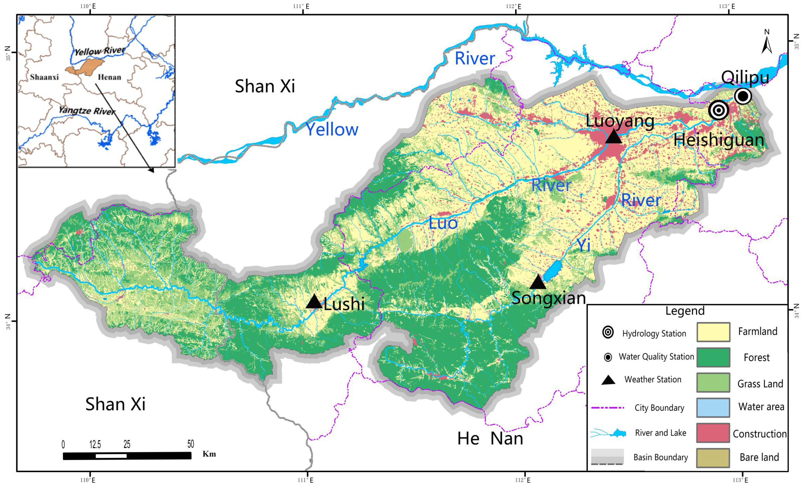
2.1. Study Site

The Yiluo River, a significant tributary of the lower Yellow River, spans a length of 974 km, flowing across 21 counties and cities in the Shanxi and Henan provinces. It consists primarily of two segments: the Yishui River (265 km) and the Luoshui River (447 km). At the outlet of the basin, the Heishiguan station serves as the control hydrological station, covering an area of 18.6 × 10³ km².

As shown in Figure 1, the Yiluo River Basin is located within the coordinates 33°39′ N~34°54′ N and 109°43′ E~113°11′ E, with elevations ranging from 92 m to 2.62 × 10³ m. The basin is situated at the transitional juncture between the subtropical and warm temperate zones, experiencing a continental monsoon climate characterized by cold, dry winters and hot, wet summers. The monsoon influence leads to significant summer rainfall, often resulting in peak runoff and potential impacts on the downstream ecosystem [13]. The high nutrient loads in the Yiluo River Basin, as identified by Liu et al. (2013) [13], primarily stem from agricultural non-point source pollution such as runoff losses of fertilizers and livestock manure. Additionally, point sources, including urban domestic sewage and industrial wastewater discharge, also contribute to the pollution in the northern regions of the Yiluo River Basin.

The Yiluo River Basin encompasses various land use categories. These include cultivated land (8.02 × 10³ km², 43.2%), forest (6.41 × 10³ km², 34.5%), grassland (2.95 × 10³ km², 15.9%), urban land (8.51 × 10³ km², 4.58%), and water bodies (335 km², 1.80%) [14]. The land use/cover data used in this study were obtained from the National Geomatics Center of China, with a resolution of 30 m and referencing the year 2020.

2.2. The Data

Between 2019 and 2020, Total Nitrogen (TN) and Total Phosphorus (TP) served as key water quality indicators at the outlet of the Qilipu station watershed, following the guidelines of the National Surface Water Quality Automatic Monitoring System. The sub-daily discharge and specific water quality monitoring data from 2019 to 2020 at the Heishiguan station on the Yiluo River were harnessed to compute the baseline pollutant flux. This crucial dataset was furnished by the Bureau of Hydrology of the Huanghe Water Resources Commission. Precipitation data (from Luoyang, Songxian, and Lushi stations) for load estimates were sourced from the National Meteorological Information Center of the China Meteorological Administration. From 2019 to 2020, the daily TN concentrations at the Qilipu station ranged from 0.868 to 18.0 mg/L, with an average of 6.76 mg/L. The TP concentrations ranged from 0.036 to 0.264 mg/L, with an average of 0.089 mg/L. The average runoff at the Heishiguan station (near to Qilipu) varied between 3.16 and 403 m³/s, with an average of 37.6 m³/s. The average annual precipitation of the basin exhibited values of 450 mm for 2019 and 618 mm for 2020.

2.3. Method

A range of calculation algorithms have been utilized to estimate nutrient loads from infrequent concentration data [15].

Table 1. List of load estimation algorithms.

Method	Algorithm	Class	Description [Reference]
M_1	$\mathrm{K}\left({\displaystyle \sum _{\mathrm{i}=1}^{\mathrm{n}}}\frac{{\mathrm{C}}_{\mathrm{i}}}{\mathrm{n}}\right)\left({\displaystyle \sum _{\mathrm{i}=1}^{\mathrm{n}}}\frac{{\mathrm{Q}}_{\mathrm{i}}}{\mathrm{n}}\right)$	Interpolation	Means of sampled concentration multiplied by discharge [21]
M_2	$\mathrm{K}\left({\displaystyle \sum _{\mathrm{i}=1}^{\mathrm{n}}}\frac{{\mathrm{C}}_{\mathrm{i}}{\mathrm{Q}}_{\mathrm{i}}}{\mathrm{n}}\right)$	Interpolation	Average of instantaneous fluxes [21]
M_3	$\mathrm{K}\mathrm{\prime }{\displaystyle \sum _{\mathrm{i}=1}^{\mathrm{n}}}{\mathrm{C}}_{\mathrm{i}}\overline{{\mathrm{Q}}_{\mathrm{l},\mathrm{l}-1}}$	Interpolation	Constant concentration before and after sampling [22]
M_4	$\mathrm{K}\overline{\mathrm{Q}}\left({\displaystyle \sum _{\mathrm{i}=1}^{\mathrm{n}}}\frac{{\mathrm{C}}_{\mathrm{i}}}{\mathrm{n}}\right)$	Interpolation	Product of the annual flow volume by the arithmetic average of the concentration [23]
M_5	$\mathrm{K}\frac{{\displaystyle {\sum }_{\mathrm{i}=1}^{\mathrm{n}}}{\mathrm{C}}_{\mathrm{i}}{\mathrm{Q}}_{\mathrm{i}}}{{\displaystyle {\sum }_{\mathrm{i}=1}^{\mathrm{n}}}{\mathrm{Q}}_{\mathrm{i}}}\overline{\mathrm{Q}}$	Interpolation	Product of the annual flow volume by the flow (at the time of sampling)-weighted average of the concentration [24]
M_6	$\mathrm{K}\mathrm{″}{\displaystyle \sum _{\mathrm{j}=1}^{\mathrm{n}}}{\mathrm{C}}_{\mathrm{j}}^{\mathrm{int}}{\mathrm{Q}}_{\mathrm{j}}$	Interpolation	Linear interpolation of concentrations multiplied by flow continuous flow [9]
M_7	$\mathrm{Q}\frac{\overline{\mathrm{l}}}{\overline{\mathrm{q}}}\left[\frac{1+\frac{1}{\mathrm{n}}\left[\frac{\mathrm{Cov}\left(\mathrm{l},\mathrm{q}\right)}{\overline{\mathrm{l}}\overline{\mathrm{q}}}\right]}{1+\frac{1}{\mathrm{n}}\left[\frac{\mathrm{Var}\left(\overline{\mathrm{q}}\right)}{\overline{{\mathrm{q}}^2}}\right]}\right]$	Ratio	M_5 corrected by a factor taking into account the covariance between the instantaneous fluxes and the flow at the time of sampling, divided by the flow variance [25]
M_8	$\mathrm{C}=\mathrm{a}{\mathrm{Q}}^{\mathrm{b}}$ ${\displaystyle \sum _{\mathrm{i}=1}^{\mathrm{n}}}{\mathrm{C}}_{\mathrm{i}}{\mathrm{Q}}_{\mathrm{i}}$	Regression	Log–log linear rating curve between concentration and flow [15,25]
M_9	$\mathrm{C}=\mathrm{a}{\mathrm{Q}}^{\mathrm{b}}$ ${\mathrm{L}}_{\mathrm{c}\mathrm{r}}={\mathrm{L}}_{\mathrm{r}}\cdot {\mathrm{e}}^{2.651{\mathrm{s}}^2}$.	Regression	Method M_8 corrected by a standard error of the estimate of rating curve in log10 units [15,19,20]

provides detailed descriptions and equations for each load estimation algorithm. The load estimation algorithms used in this study can be categorized into three main groups: interpolation methods (M_1, M_2, M_3, M_4, M_5, and M_6), which estimate loads by interpolating between measured concentrations; ratio methods (M_7), which calculate loads using the ratio of the average load to the average flow; and regression methods (M_8 and M_9), which establish a regression relationship between concentration and flow to estimate loads. In this study, we employed the algorithms commonly cited in the literature to estimate nutrient load [9,16,17,18] and the nine load estimation methods (M_1-M_9) listed in Table 1 using the Python programming language. Specifically, the NumPy (https://numpy.org/devdocs/index.html, accessed on 10 May 2024) and Pandas libraries (https://pandas.pydata.org/, accessed on 10 May 2024) were used for data processing and calculation, while the Matplotlib and Seaborn libraries (https://matplotlib.org/, accessed on 10 May 2024) were employed for data visualization. C_i (mg/L) represents the instantaneous concentration associated with individual samples, Q_i (m³/s) denotes the instantaneous discharge at the time of sampling, n is the number of samples collected, Q_i,i−1 signifies the discharge for Q_i and Q_i−1, and $\overline{\mathrm{Q}}$ is the average discharge for the period of record. C_jint (mg/L) is the daily concentration linearly interpolated between two measured samples, K is a conversion factor to account for the period of load estimation, and $\overline{l}$ (g/s) is the mean flow, with s representing the standard error of the estimate of the rating curve in log₁₀ units. Regression Method M_8 corrected by a standard error of the estimate of rating curve in log10 units [15,19,20].

A benchmark nutrient load was computed for the observed site using nutrient concentrations and continuous discharge measurements. By multiplying the average daily nutrient concentration data with the daily volumetric discharge, the load was determined. Extreme events are defined as days when the daily streamflow exceeded the 95th percentile of the observed daily streamflow record at the Heishiguan gauging station (calculated as the value of 82.5 m³/s). During the study period (2019–2020), we identified a total of 37 extreme events, with 9 events occurring in 2019 and 28 events in 2020 (Table S1).

2.4. Sampling Scenarios

To investigate the impact of sampling frequency on seasonal and annual load estimates, we employed Monte Carlo simulations to subsample our reference dataset. Given that a variety of sampling strategies could be explored (e.g., fixed period, flow proportional), we opted for fixed-period sampling due to its common use in water quality monitoring programs. The simulation of sampling frequencies was performed using the Monte Carlo method, implemented by Python code. First, a starting date was randomly selected from the reference dataset, and then samples were extracted at specified intervals (e.g., 3 days, 7 days, etc.) to obtain a robust distribution of results after 10thousands iterations [16,26].

2.5. Calculating Uncertainty

The uncertainty in nutrient load estimates is defined as the difference between the reference load and the estimated load [16,27]. This is often expressed as a percentage deviation from the reference load. We compared TP and TN load estimates from various calculation algorithms and sampling frequencies to the load derived from the daily reference datasets. The Mean Relative Error (MRE) was calculated as:

$$\mathit{MRE}=\frac{(L_{\mathit{estimate}}-L_{\mathit{reference}})}{L_{\mathit{reference}}}\times 100$$

(1)

where $L_{\mathit{estimate}}$ represents the estimated flux, and $L_{\mathit{reference}}$ represents the observed flux. An $E_{\mathit{relative} \mathit{error}}$ of 0 indicates that the estimated and observed fluxes are equal, while an MRE < 0 indicates underestimation and an MRE > 0 indicates overestimation by the regression model. We obtained the daily observed export flux for TN or TP at the watershed mouth using a standard algorithm based on the instantaneous flow discharge and daily concentration (Equation (1)).

$$\mathit{STD}=\frac{\sqrt{\frac{\sum _1^n{(L_{\mathit{estimate}}-L_{\mathit{reference}})}^2}{N}}}{L_{\mathit{reference}}}\times 100$$

(2)

The Standard Deviation of the Percentage errors (STD) was calculated as Equation (2).

3. Results

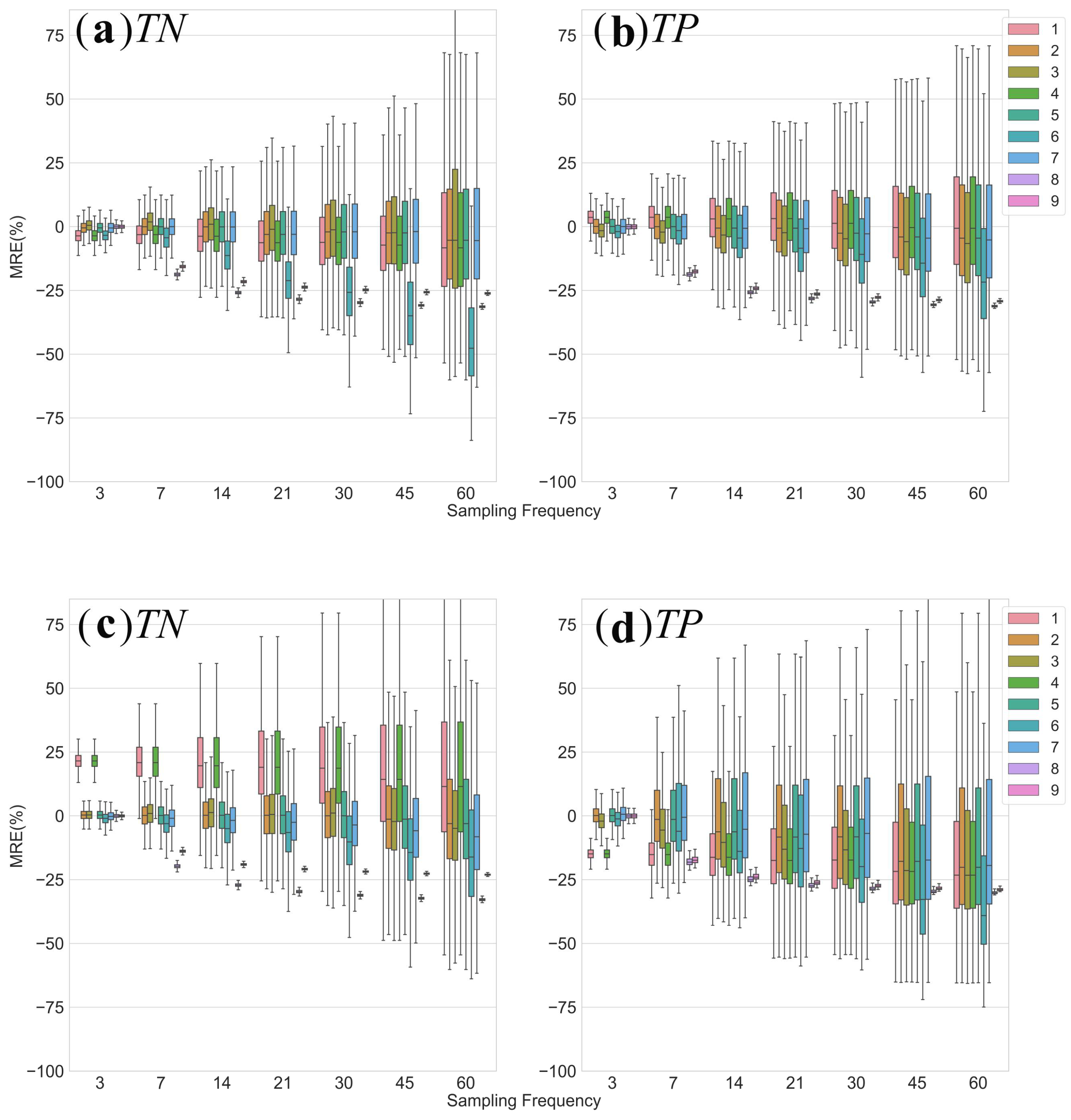
3.1. Influence of Sampling Frequency and Calculation Methods on Annual Load Estimates

The accuracy of annual nutrient load estimates varied notably across different calculation methods and sampling frequencies (as shown in Figure 2, Tables S2 and S3). A decrease in sampling frequency led to a marked increase in the uncertainty of these estimates, as evidenced by the range of STD (Table S2) and MRE (Table S3). The 3-day sampling frequency showed the highest accuracy for both TN and TP load estimates, with STD ranging from 0.598 to 22. 9% and 1.10 to 18.7%, respectively. However, this value increased to 21.0–48.0% for TN and 25.1–67.7% for TP at a 60-day sampling frequency. Among the nine calculation methods, M_8 and M_9 generally had the lowest STD for both TP and TN estimates across all sampling frequencies. There are notable discrepancies between the performance of methods M_1, M_4, and the other methods for Total Nitrogen (TN) load estimates in the year 2020. While the STD values for M_2, M_3, M_5, M_6, and M_7 range from 1.99% to 29.4% across the various sampling frequencies in 2020, the STD values for M_1 and M_4 are substantially higher, ranging from 21. 9% to 45.6%. The M_1 and M_4, which rely on the arithmetic average of sampled concentrations and the product of annual flow volume and the arithmetic average of the concentration, respectively, may not effectively represent the complex relationship between concentration and discharge, especially during high-flow events or periods of extreme variability.

There are substantial variations in the MRE values for methods M_1, M_4, M_8, and M_9 compared to the other methods in the year 2020 (Figure 2 and Table S3). For TN load estimates, M_1 and M_4 show consistently high MRE values, ranging from 21.0% to 22.6%, while the other methods (M_2, M_3, M_5, M_6, and M_7) have much lower MRE values, ranging from −4.71% to 1.71%. Similarly, for TP load estimates, M_1 and M_4 have large negative MRE values, ranging from −14.8% to −13.4%, whereas the other methods show a mix of positive and negative MRE values with smaller magnitudes.

In summary, low-frequency sampling led to high uncertainties in annual load estimates. Selecting optimized models like M_3 and M_7 and increasing sampling frequency to at least once per two weeks can effectively control estimation errors within about ±20% for both TP and TN. The differences between the two study years were also evident, with generally higher estimation errors in 2020 than 2019. It is important to note that the results of annual load estimates may be influenced by several methodological considerations or limitations [28]. The quality and accuracy of the input data, such as discharge measurements and nutrient concentration analyses, can affect the reliability of load estimates. Measurement errors or biases in these data sources can propagate through the estimation process and contribute to uncertainty. Moreover, the assumptions underlying the different estimation methods, such as the existence of a stable concentration–discharge relationship or the representativeness of sampling points, may not always hold true in real-world conditions [29].

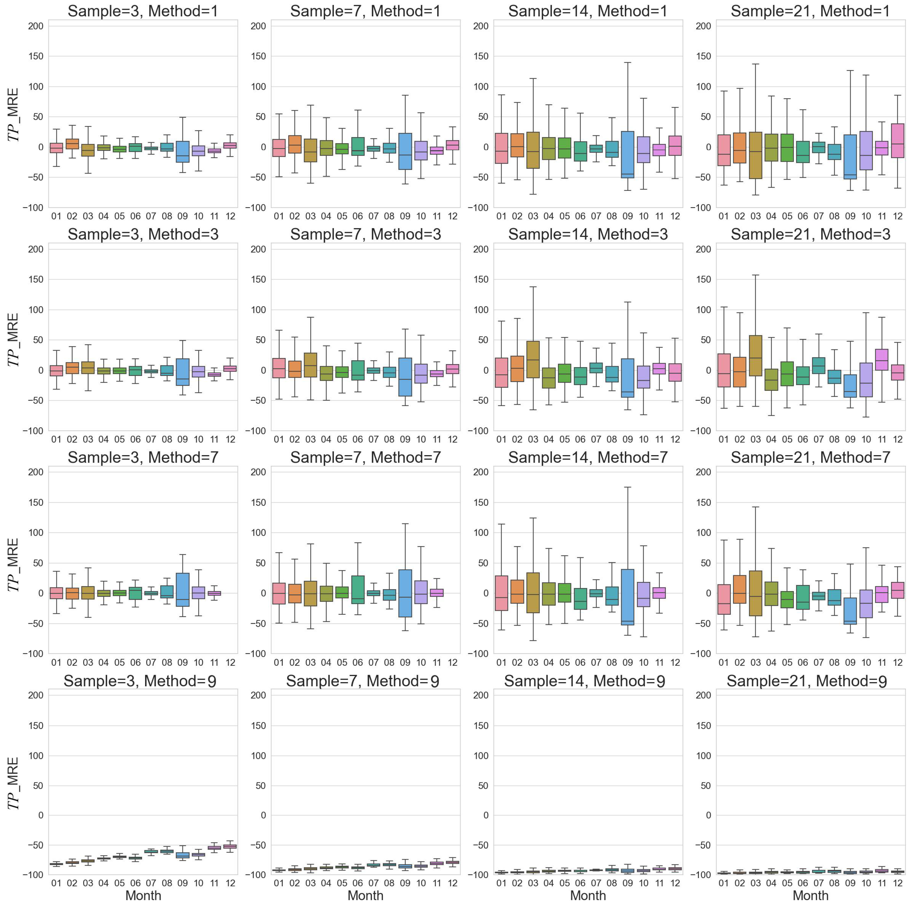
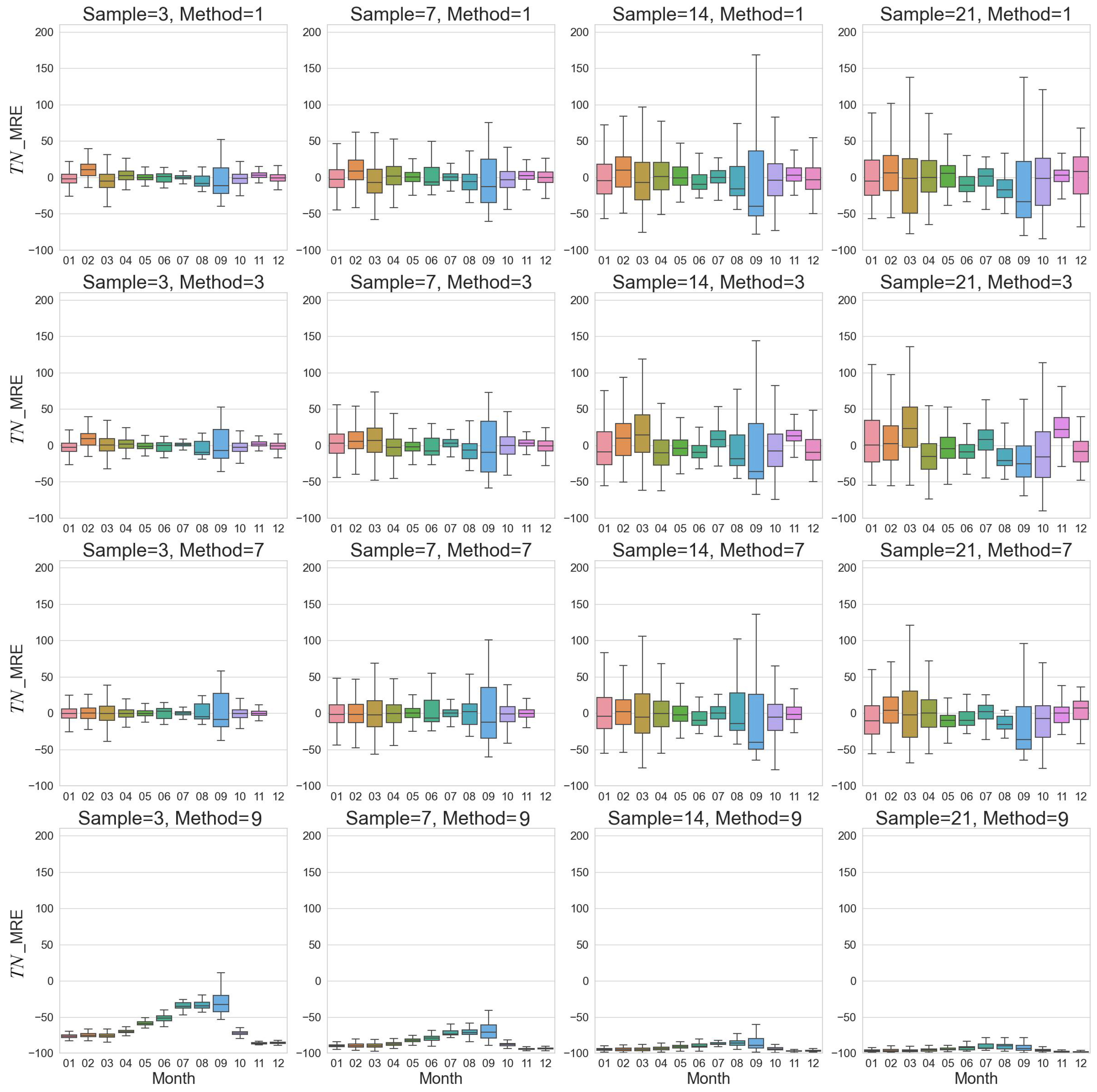
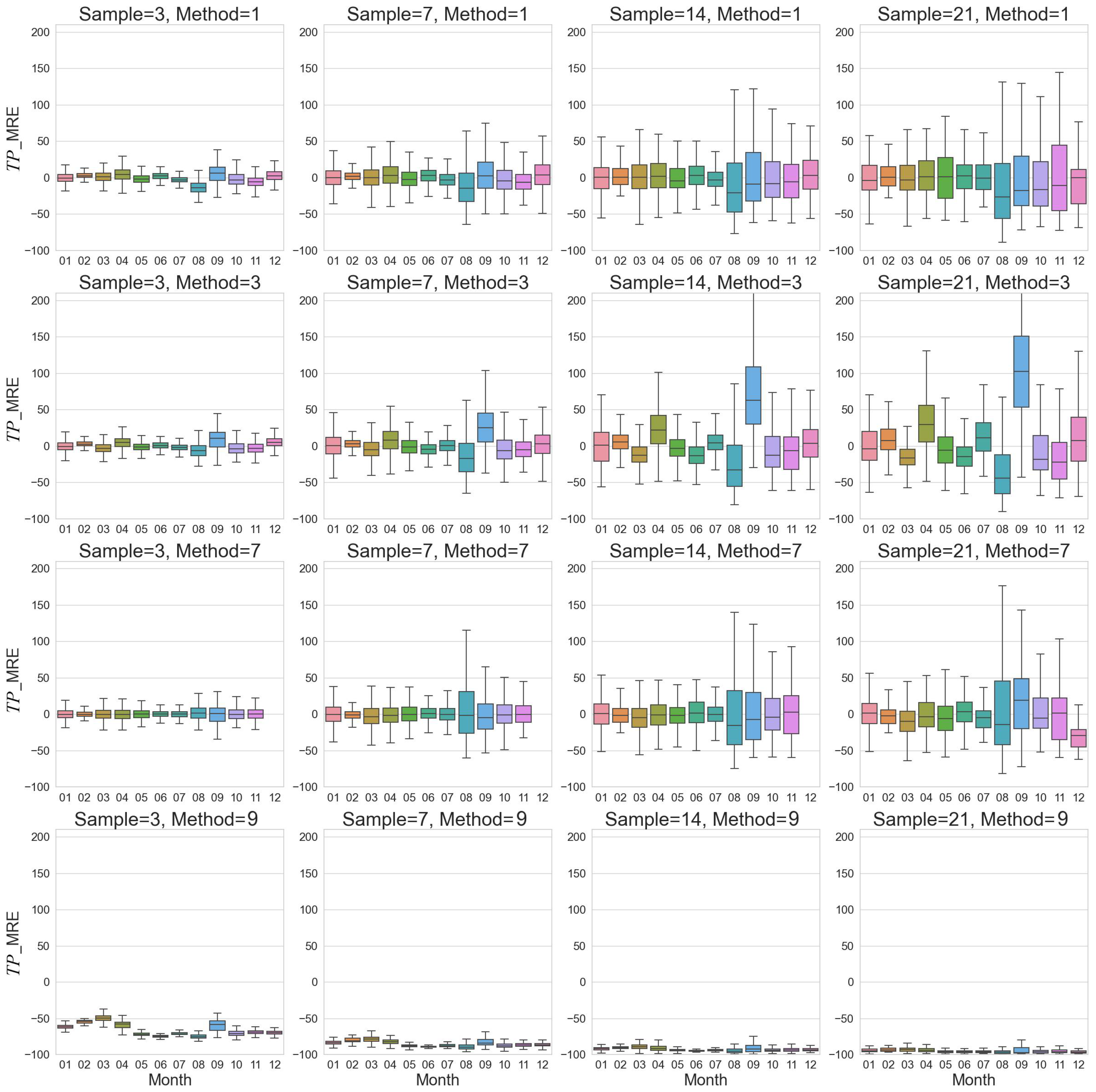
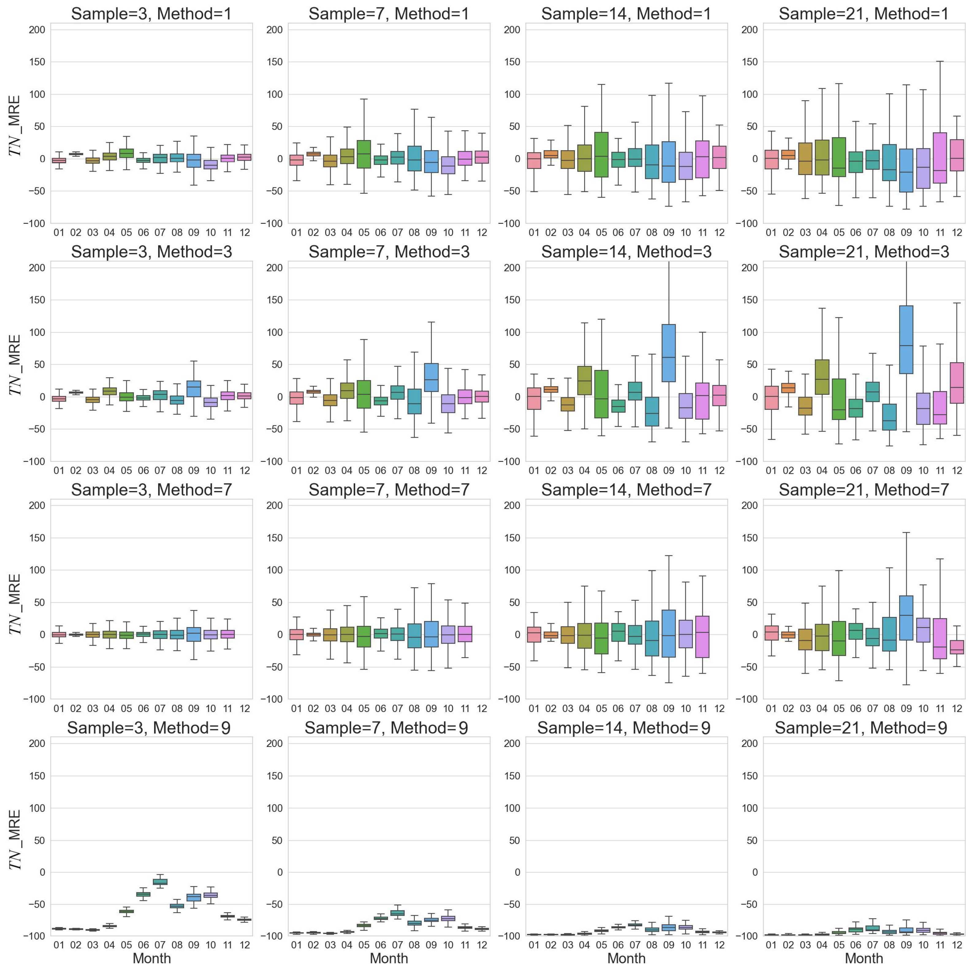
3.2. Seasonal Variations in Load Estimates Uncertainties and Potential Influencing Factors

For TP load estimates, the probability of MRE exceeding ±10% was below 50% for 3-day and 7-day sampling frequencies, but higher than 50% for 14-day and 30-day frequencies in most months (Figure 3 and Figure S1). The MRE of monthly TP load estimates ranged 3.39–3.96% for 3-day sampling, but increased to 24.5–61.2% for 60-day sampling (Table S2), indicating a notable decrease in estimation precision with reduced sampling frequency.

The estimation errors showed clear temporal variations and seasonal differences for all sampling frequencies. MRE values were generally higher in 2020 than in 2019 (Figure 3, Figure 4, Figure 5 and Figure 6 and Figures S1–S4), especially for lower sampling frequencies, which might be related to more frequent occurrence of storm events in 2020. Error magnitudes increased notably during the high-flow season from June to September, resulting in much higher MRE compared to other months.

Methods M_4 and M_5 performed the worst in the spring months (May, June), with MRE exceeding 50%, while M_3 and M_7 had consistently lower MRE (<30%) throughout the year (Figure 5, Figure 6 and Figures S3 and S4). The poorer performance of M_4 and M_5 might be attributed to their inability to capture the rapid changes in hydrological processes and nutrient concentrations during the wet season with frequent storm events.

Figure 3, Figure 4, Figure 5 and Figure 6 and Figures S1–S4 show the changes in MRE of estimated monthly TN and TP export fluxes at different sampling frequencies and calculation methods. In general, the estimation errors of various methods at low sampling frequencies were considerably higher than those at high sampling frequencies, especially during the flood season and months with frequent extreme events. The performance of different methods also varied, with M_3 and M_7 exhibiting relatively higher stability and accuracy across sampling frequencies, while M_4 and M_5 had larger errors during spring and the flood season. These results suggest that selecting an appropriate sampling frequency and estimation method is crucial for reducing the uncertainty of load estimation at the monthly scale, particularly by increasing the sampling frequency during the flood season and extreme events and choosing nonlinear methods that can better characterize the flow–concentration relationship.

3.3. Impacts of Extreme Events on Nutrient Export and Its Seasonal Patterns

Extreme events substantially influenced the dynamics of TN and TP nutrient exports. Particularly in 2020, days with extreme flow rates accounted for only 7.650% of the year (28 days out of 366 days) but contributed 38.105% of the annual TP load (Figure 7).

The magnitudes of streamflow and nutrient concentration extremes differed between the two years. As shown in Figure 7a,b, the top 20% of TP concentrations were higher in 2019 (>0.150 mg/L) than in 2020 (>0.080 mg/L), while the top 5–20% of TN concentrations were higher in 2020 (12.500 mg/L) than in 2019 (7.500 mg/L). Nutrient concentrations showed higher probability of co-occurrence with streamflow during summer in 2020 (Figure 7g), indicating hydrologically driven export. However, the relationships were more variable in 2019, suggesting the contribution of other factors such as land use and agricultural activities. The notable increase in TN concentration at the end of 2019 and the beginning of 2020 (Figure 7b) might be related to winter agricultural activities (e.g., fertilizer application) and the concentration effect caused by reduced runoff (Figure 7c). Seasonal variations in nutrient concentrations play a key role in understanding the variability in nutrient export fluxes [30,31]. As shown in Figure 7a,b, both TN and TP concentrations exhibited distinct seasonal differences and inter-annual variations. The sustained decrease in nutrient concentrations during most of 2019 could be attributed to the implementation of watershed management measures, vegetation restoration, and increased runoff (Figure 7c), while the concentration peaks in 2020 were mainly influenced by extreme hydrological events (Figure 7c,f). The cumulative curves for TN and TP load (Figure 7d,e) further illustrate the differences in nutrient export dynamics between the two years, with a more pronounced increase in cumulative loads during high-flow events in 2020 compared to 2019. These seasonal and inter-annual variation patterns have important implications for optimizing sampling strategies and selecting estimation methods.

4. Discussion

4.1. Optimal Methods for Estimating Nutrient Loads

This study evaluated nine commonly used methods for estimating riverine nutrient loads and found that methods M_3 and M_7 generally provided the most accurate estimates for both TN and TP loads at various sampling frequencies. M_3 and M_7 had the lowest STD (Figure 3, Figure 4, Figure 5 and Figure 6 and Tables S2 and S3) and MRE values at a biweekly sampling interval for annual load estimation. This is consistent with previous studies that also recommended M_3 and M_7 for estimating nitrogen and phosphorus loads in agricultural watersheds [9,11,16]. The good performance of M_3 and M_7 can be attributed to their ability to account for the covariation between constituent concentrations and streamflow. In contrast, methods like M_4 may overestimate loads during high-flow periods due to dilution effects [32,33]. However, it should be noted that the performance of different methods may vary depending on the catchment characteristics and sampling strategies. For example, Kronvang and Bruhn (1996) found that M_3 and M_7 performed better in large agricultural catchments (greater than 100 km²), but their advantage diminished in smaller catchments (less than 50 km²) [33]. Therefore, the selection of load estimation methods should consider the specific hydrological and land use conditions of the study watershed.

Our findings also contribute to the growing body of literature comparing different load estimation techniques across various watershed settings [9,11,16,32,33]. While previous studies have primarily focused on evaluating a limited number of methods or sampling strategies [9,11,16], our comprehensive assessment of nine estimation methods and seven sampling frequencies provides a more holistic perspective on their relative performance. Moreover, by conducting the analysis in an agricultural watershed dominated by non-point source pollution, we address an important gap in understanding the influence of land use and pollution sources on load estimation uncertainty. The consistent performance of M_3 and M_7 across different sampling frequencies and hydrological conditions highlights their robustness and suitability for application in similar agricultural watersheds.

4.2. Optimum Sampling Strategy for Load Estimation

Our results showed that sampling frequency had a greater influence on the accuracy of annual nutrient load estimates than the choice of estimation methods. The uncertainties in annual TN and TP load estimates increased dramatically as sampling intervals increased from 3 days to 60 days (Figure 2). This highlights the importance of selecting an appropriate sampling frequency that can capture the temporal variability in nutrient concentrations and loads. Infrequent sampling may miss important high-flow events that transport a large proportion of annual loads [18,34].

The optimal sampling frequency should strike a balance between monitoring objectives, accuracy requirements, and resource constraints [16,21]. For the Yiluo River watershed, we found that a biweekly sampling strategy with M_7 could provide relatively accurate estimates of annual TN loads (STD < 10%), while a weekly sampling strategy was needed for TP load estimates. M_7 maintains the MRE within ±20% when sampling biweekly (Figure 7). This is in line with the sampling frequency recommended by Moatar and Meybeck (2005) [9] for different nutrient constituents. A higher frequency may be required for dissolved reactive phosphorus due to its more dynamic behavior [11].

To further improve the accuracy of load estimates while minimizing the monitoring cost, composite sampling strategies can be used [19]. For example, flow-proportional sampling or stratified sampling with more frequent sampling during high-flow periods can better capture the variability in nutrient concentrations and loads. The sampling strategy should also be adaptive to inter-annual and seasonal variations in hydrological conditions. It is also crucial to consider its specific characteristics, such as the dominant land use types, pollution sources, and hydrological regime. Agricultural watersheds like the Yiluo River Basin may require more frequent sampling during the growing season and storm events due to the high variability in nutrient loads driven by agricultural activities and surface runoff.

Furthermore, the sampling strategy should be designed in line with the management objectives and the desired level of accuracy in load estimates. If the goal is to quantify long-term nutrient loading trends and assess the effectiveness of watershed management practices, a lower sampling frequency may be sufficient. However, if the objective is to capture short-term variability in nutrient dynamics or to support real-time decision-making, higher-frequency sampling will be necessary. The choice of sampling strategy should also consider the trade-offs between data resolution, accuracy, and monitoring costs. While higher sampling frequencies generally improve load estimation accuracy, they also entail higher labor and analytical costs. Balancing these factors is essential for designing cost-effective monitoring programs that provide the necessary information for watershed management while optimizing resource allocation.

4.3. Impact of Storm Events on Load Estimation

Extreme rainfall and runoff events played a critical role in driving riverine nutrient export in the Yiluo River watershed. Around half of the annual TN and TP loads were delivered in less than 20% of the time during a few extreme events (Figure 7). This is consistent with many previous studies showing the disproportionate contribution of extreme events to nutrient loads [11,34]. The elevated MRE values for lower sampling frequencies in 2020 can be attributed to the more frequent occurrence of storm events and the associated high variability in TP concentrations and loads during these months. The inability of low-frequency sampling to capture the rapid fluctuations in TP dynamics during storm events likely contributed to the higher estimation errors. Comparing the MRE patterns between 2019 and 2020 reveals that the estimation errors were generally higher in 2020 across all sampling frequencies and methods. This difference highlights the influence of inter-annual variability in hydrological conditions on the accuracy of TP load estimates.

The impact of extreme events on load estimates also varied between nutrients and sampling frequencies. TP loads were more strongly affected by extreme events than TN loads. With a 60-day sampling interval, the probability of relative errors exceeding 10% was 77.8–100% for TN and 66.7–100% for TP (Figure 2). This can be explained by the different transport mechanisms and sources of nitrogen and phosphorus. Phosphorus is often associated with sediments and particulates that are mobilized during high-flow events, while nitrogen transport is more related to subsurface flow and groundwater inputs [18].

The large uncertainties in load estimates caused by extreme events underscore the need to adjust sampling strategies to better capture these important periods. Increasing sampling frequency during high-flow seasons and events can notably improve load estimates [21]. In addition, event-based sampling or real-time sensors may be used to capture the high-resolution dynamics of nutrient transport during storm events [33].

The impact of extreme events on nutrient load estimation also has important implications for watershed management. The high proportion of annual loads delivered during short periods highlights the need for best management practices (BMPs) that can mitigate nutrient losses during these critical times. For example, cover crops, riparian buffers, and wetlands can help reduce nutrient export during storm events by enhancing nutrient retention and reducing surface runoff [28,35,36]. Targeted implementation of these BMPs in hotspots of nutrient loss, such as areas with high soil erosion rates or intensive agricultural activities, can be an effective strategy for reducing overall nutrient loads. Moreover, the large uncertainties in load estimates during extreme events emphasize the importance of collecting high-frequency monitoring data to support watershed modeling efforts. Many watershed models rely on nutrient load estimates for calibration and validation, and inaccurate load estimates can lead to poor model performance and unreliable predictions of the effectiveness of management practices [37]. High-resolution monitoring data collected during storm events can help improve model parameterization and reduce uncertainties in model predictions, enabling better-informed decision-making for watershed management.

4.4. Selecting a Sampling Strategy to Minimize Uncertainty in Nutrient Loads

This study demonstrated that the choice of sampling strategy and load estimation method can considerably affect the accuracy of riverine nutrient load estimates, which are critical for guiding watershed management and assessing environmental impacts. The optimal monitoring approach should consider the trade-offs between data resolution, accuracy, and cost based on the management objectives and watershed characteristics [13,23]. The large contribution of extreme events to annual loads also highlights the importance of best management practices (BMPs) that can mitigate nutrient losses during these high-risk periods, such as cover crops, riparian buffers, and wetlands [11]. Monitoring data with sufficient temporal resolution during storm events is also crucial for calibrating and validating watershed models that can simulate the effectiveness of different BMPs and inform adaptive management [34].

5. Conclusions

The results of this study showed that infrequent sampling can lead to notable errors in both annual and seasonal load estimates, with the performance of different estimation methods varying across sampling frequencies. To improve load estimation accuracy, it is essential to increase sampling frequency during high-flow periods and select methods that can better characterize the concentration–discharge relationships, such as the flow-weighted concentration method M_7 with a biweekly sampling frequency that provided the most accurate estimates for both TN and TP loads, while monthly sampling had the largest errors. Extreme events were found to be critical drivers of nutrient export, contributing to around half of the annual TN and TP loads in less than 20% of the time. The impact of extreme events on load estimates varied between nutrients and sampling frequencies, with TP loads being more sensitive than TN loads. Therefore, sampling strategies should be adapted to better capture these high-flow periods, such as increasing sampling frequency during the wet season and utilizing methods that can better characterize the concentration–discharge relationships. To improve the accuracy of load estimates, we recommend a minimum sampling frequency of once per two weeks with the M_7 method for the Yiluo River watershed and similar agricultural catchments. However, adaptive monitoring approaches that adjust sampling frequencies based on hydrological conditions and target extreme events are highly encouraged. Furthermore, incorporating the effects of watershed human activities is important for understanding the seasonal patterns of nutrient export.

By adopting more accurate and cost-effective sampling strategies, resources can be focused on critical periods and processes, thus avoiding unnecessary costs and improving the overall performance of monitoring and modeling efforts. However, this study has limitations in the range of estimation methods evaluated, such as LOADEST, WRTDS, and machine learning approaches, and does not consider the impact of land use and climate change on nutrient export dynamics, despite their potential influence on nutrient loading and the performance of estimation methods. Future research should explore more advanced estimation techniques, investigate the effects of environmental changes on nutrient export processes, and develop adaptive monitoring strategies to account for the non-stationary nature of nutrient dynamics. Based on the limitations of the current study, future research should: (1) explore advanced load estimation techniques, such as machine learning and Bayesian methods, that are more robust to data limitations and assumptions, particularly during extreme events and non-stationary conditions; (2) investigate the effects of climate change and land use/cover changes on nutrient export dynamics and load estimation uncertainties, as these factors can alter nutrient delivery timing, magnitude, and concentration–discharge relationships; (3) develop adaptive monitoring strategies that account for the non-stationary nature of nutrient dynamics and optimize sampling efforts using real-time data, high-frequency sensors, remote sensing, and modeling to improve load estimation accuracy while minimizing costs. Addressing these directions will advance our understanding of the complex nature of riverine nutrient export and provide robust and cost-effective monitoring strategies for watershed management in a changing environment.

References

1. Van der Grift, B.; Broers, H.P.; Berendrecht, W.; Rozemeijer, J.; Osté, L.; Griffioen, J. High-Frequency Monitoring Reveals Nutrient Sources and Transport Processes in an Agriculture-Dominated Lowland Water System. Hydrol. Earth Syst. Sci. 2016, 20, 1851–1868. [Google Scholar] [CrossRef]
2. Birgand, F.; Faucheux, C.; Moatar, F.; Meybeck, M. Uncertainties on Nitrate Water Quality Indicators Associated with Infrequent Sampling in Brittany, France. In Proceedings of the 2009 American Society of Agricultural and Biological Engineers(ASABE), Annual International Meeting, Reno, NV, USA, 21–24 June 2009; American Society of Agricultural and Biological Engineers: St. Joseph, MI, USA, 2009; p. 1. [Google Scholar]
3. Verma, S.; Markus, M.; Cooke, R.A. Development of Error Correction Techniques for Nitrate-N Load Estimation Methods. J. Hydrol. 2012, 432, 12–25. [Google Scholar] [CrossRef]
4. Liang, K.; Jiang, Y.; Meng, F.-R. Large Discrepancies on Nitrate Loading Estimates from Sparse Measurements by SWAT and Statistical Models at Catchment Scale. In Proceedings of the EGU General Assembly Conference Abstracts, Online, 19–30 April 2021; p. EGU21-10458. [Google Scholar]
5. Park, D.; Um, M.-J.; Markus, M.; Jung, K.; Keefer, L.; Verma, S. Insights from an Evaluation of Nitrate Load Estimation Methods in the Midwestern United States. Sustainability 2021, 13, 7508. [Google Scholar] [CrossRef]
6. Mosquin, P.L.; Aldworth, J.; Chen, W. Evaluation of the Use of Bias Factors with Water Monitoring Data. Environ. Toxicol. Chem. 2018, 37, 1864–1876. [Google Scholar] [CrossRef] [PubMed]
7. Lee, C.J.; Hirsch, R.M.; Crawford, C.G. An Evaluation of Methods for Computing Annual Water-Quality Loads; U.S. Geological Survey: Reston, VA, USA, 2019. [Google Scholar]
8. Li, J.; Tian, L.; Wang, Y.; Jin, S.; Li, T.; Hou, X. Optimal Sampling Strategy of Water Quality Monitoring at High Dynamic Lakes: A Remote Sensing and Spatial Simulated Annealing Integrated Approach. Sci. Total Environ. 2021, 777, 146113. [Google Scholar] [CrossRef]
9. Moatar, F.; Meybeck, M. Compared Performances of Different Algorithms for Estimating Annual Nutrient Loads Discharged by the Eutrophic River Loire. Hydrol. Process. 2005, 19, 429–444. [Google Scholar] [CrossRef]
10. Jiang, Y.; Frankenberger, J.R.; Bowling, L.C.; Sun, Z. Quantification of Uncertainty in Estimated Nitrate-N Loads in Agricultural Watersheds. J. Hydrol. 2014, 519, 106–116. [Google Scholar] [CrossRef]
11. Williams, M.R.; King, K.W.; Macrae, M.L.; Ford, W.; Van Esbroeck, C.; Brunke, R.I.; English, M.C.; Schiff, S.L. Uncertainty in Nutrient Loads from Tile-Drained Landscapes: Effect of Sampling Frequency, Calculation Algorithm, and Compositing Strategy. J. Hydrol. 2015, 530, 306–316. [Google Scholar] [CrossRef]
12. Worrall, F.; Howden, N.; Burt, T. Assessment of Sample Frequency Bias and Precision in Fluvial Flux Calculations–An Improved Low Bias Estimation Method. J. Hydrol. 2013, 503, 101–110. [Google Scholar] [CrossRef]
13. Liu, X.; Dai, X.; Zhong, Y.; Li, J.; Wang, P. Analysis of Changes in the Relationship between Precipitation and Streamflow in the Yiluo River, China. Theor. Appl. Climatol. 2013, 114, 183–191. [Google Scholar] [CrossRef]
14. Hou, J.; Qin, T.; Liu, S.; Wang, J.; Dong, B.; Yan, S.; Nie, H. Analysis and Prediction of Ecosystem Service Values Based on Land Use/Cover Change in the Yiluo River Basin. Sustainability 2021, 13, 6432. [Google Scholar] [CrossRef]
15. Phillips, J.; Webb, B.; Walling, D.; Leeks, G. Estimating the Suspended Sediment Loads of Rivers in the LOIS Study Area Using Infrequent Samples. Hydrol. Process. 1999, 13, 1035–1050. [Google Scholar] [CrossRef]
16. Birgand, F.; Faucheux, C.; Gruau, G.; Augeard, B.; Moatar, F.; Bordenave, P. Uncertainties in Assessing Annual Nitrate Loads and Concentration Indicators: Part 1. Impact of Sampling Frequency and Load Estimation Algorithms. Trans. ASABE 2010, 53, 437–446. [Google Scholar] [CrossRef]
17. Cassidy, R.; Jordan, P. Limitations of Instantaneous Water Quality Sampling in Surface-Water Catchments: Comparison with near-Continuous Phosphorus Time-Series Data. J. Hydrol. 2011, 405, 182–193. [Google Scholar] [CrossRef]
18. Defew, L.; May, L.; Heal, K. Uncertainties in Estimated Phosphorus Loads as a Function of Different Sampling Frequencies and Common Calculation Methods. Mar. Freshw. Res. 2013, 64, 373–386. [Google Scholar] [CrossRef]
19. Quilbé, R.; Rousseau, A.N.; Duchemin, M.; Poulin, A.; Gangbazo, G.; Villeneuve, J.-P. Selecting a Calculation Method to Estimate Sediment and Nutrient Loads in Streams: Application to the Beaurivage River (Québec, Canada). J. Hydrol. 2006, 326, 295–310. [Google Scholar] [CrossRef]
20. Ferguson, R. River Loads Underestimated by Rating Curves. Water Resour. Res. 1986, 22, 74–76. [Google Scholar] [CrossRef]
21. Reynolds, K.N.; Loecke, T.D.; Burgin, A.J.; Davis, C.A.; Riveros-Iregui, D.; Thomas, S.A.; St. Clair, M.A.; Ward, A.S. Optimizing Sampling Strategies for Riverine Nitrate Using High-Frequency Data in Agricultural Watersheds. Environ. Sci. Technol. 2016, 50, 6406–6414. [Google Scholar] [CrossRef]
22. Preston, S.D.; Bierman Jr, V.J.; Silliman, S.E. An Evaluation of Methods for the Estimation of Tributary Mass Loads. Water Resour. Res. 1989, 25, 1379–1389. [Google Scholar] [CrossRef]
23. Walling, D.E.; Webb, B.W. Estimating the Discharge of Contaminants to Coastal Waters by Rivers: Some Cautionary Comments. Mar. Pollut. Bull. 1985, 16, 488–492. [Google Scholar] [CrossRef]
24. Shih, G.; Abtew, W.; Obeysekera, J. Accuracy of Nutrient Runoff Load Calculations Using Time-Composite Sampling. Trans. ASAE 1994, 37, 419–429. [Google Scholar] [CrossRef]
25. Littlewood, I.G. Estimating Contaminant Loads in Rivers: A Review; Institute of Hydrology: Uttarakhand, Italy, 1992. [Google Scholar]
26. Richards, R.P.; Holloway, J. Monte Carlo Studies of Sampling Strategies for Estimating Tributary Loads. Water Resour. Res. 1987, 23, 1939–1948. [Google Scholar] [CrossRef]
27. Harmel, R.; Cooper, R.; Slade, R.; Haney, R.; Arnold, J. Cumulative Uncertainty in Measured Streamflow and Water Quality Data for Small Watersheds. Trans. ASABE 2006, 49, 689–701. [Google Scholar] [CrossRef]
28. Li, W.; Lei, Q.; Yen, H.; Zhai, L.; Hu, W.; Li, Y.; Wang, H. Investigation of watershed nutrient export affected by extreme events and the corresponding sampling frequency. J. Environ. Manag. 2019, 250, 109477. [Google Scholar] [CrossRef]
29. Goswami, A.; Paul, P.K.; Rudra, R.; Goel, P.K. Evaluation of statistical models: Perspective of water quality load estimation. J. Hydrol. 2023, 616, 128721. [Google Scholar] [CrossRef]
30. Iital, A.; Klõga, M.; Pihlak, M.; Pachel, K.; Zahharov, A.; Loigu, E. Nitrogen content and trends in agricultural catchments in Estonia. Agr. Ecosyst. Environ. 2014, 198, 44–53. [Google Scholar] [CrossRef]
31. Rattan, K.J.; Corriveau, J.C.; Brua, R.B.; Culp, J.M.; Yates, A.G.; Chambers, P.A. Quantifying seasonal variation in total phosphorus and nitrogen from prairie streams in the Red River Basin, Manitoba Canada. Sci. Total Environ. 2017, 575, 649–659. [Google Scholar] [CrossRef]
32. Elwan, A.; Singh, R.; Patterson, M.; Roygard, J.; Horne, D.; Clothier, B.; Jones, G. Influence of Sampling Frequency and Load Calculation Methods on Quantification of Annual River Nutrient and Suspended Solids Loads. Environ. Monit. Assess. 2018, 190, 78. [Google Scholar] [CrossRef]
33. Kronvang, B.; Bruhn, A. Choice of Sampling Strategy and Estimation Method for Calculating Nitrogen and Phosphorus Transport in Small Lowland Streams. Hydrol. Process. 1996, 10, 1483–1501. [Google Scholar] [CrossRef]
34. Jones, A.S.; Horsburgh, J.S.; Mesner, N.O.; Ryel, R.J.; Stevens, D.K. Influence of Sampling Frequency on Estimation of Annual Total Phosphorus and Total Suspended Solids Loads 1. J. Am. Water Resour. Assoc. 2012, 48, 1258–1275. [Google Scholar] [CrossRef]
35. Carpenter, S.R.; Booth, E.G.; Kucharik, C.J. Extreme precipitation and phosphorus loads from two agricultural watersheds. Limnol. Oceanogr. 2018, 63, 1221–1233. [Google Scholar] [CrossRef]
36. Ezzati, G.; Kyllmar, K.; Barron, J. Long-term water quality monitoring in agricultural catchments in Sweden: Impact of climatic drivers on diffuse nutrient loads. Sci. Total Environ. 2023, 864, 160978. [Google Scholar] [CrossRef]
37. Lu, C.; Zhang, J.; Tian, H.; Crumpton, W.G.; Helmers, M.J.; Cai, W.J.; Hopkingson, C.S.; Lohrenz, S.E. Increased extreme precipitation challenges nitrogen load management to the Gulf of Mexico. Commun. Earth Environ. 2020, 1, 21. [Google Scholar] [CrossRef]
Figure 1. The location of the Yiluo River watershed, the land use types of underlying surface and water quality and runoff monitoring site in the Yiluo River watershed.
Water 16 01506 g001
Figure 2. Annual variation in TP and TN flux MRE (%) estimated by different sample frequencies and different algorithms for 2019 (up) and 2020 (down). Note: The boxes represent the interquartile range (25th to 75th percentile), the horizontal lines within the boxes indicate the median, the whiskers extend to the data points not considered outliers, and the dots represent outliers. (a) TN. (b) TP (c) TN (d) TP.
Water 16 01506 g002
Figure 3. Monthly changes in TP flux MRE estimated by different sample frequencies and different algorithms for 2019. Boxes represent the interquartile range (25th to 75th percentile), horizontal lines within the boxes indicate the median, whiskers extend to the data points not considered outliers, and dots represent outliers.
Water 16 01506 g003
Figure 4. Monthly changes in TN flux MRE estimated by different sample frequencies and different algorithms for 2019.
Water 16 01506 g004
Figure 5. Monthly changes in TP flux MRE estimated by different sample frequencies and different algorithms for 2020.
Water 16 01506 g005
Figure 6. Monthly changes in TN flux MRE estimated by different sample frequencies and different algorithms for 2020.
Water 16 01506 g006
Figure 7. Frequency of (a) TP and (b) TN concentrations, (c) runoff, (d) TP and (e) TN load, (f) precipitation, and (g) seasonal changes of flow and nutrient concentrations.
Water 16 01506 g007