Assessment of Rainfall and Temperature Trends in the Yellow River Basin, China from 2023 to 2100

Abstract

China’s Yellow River Basin (YRB) is sensitive to climate change due to its delicate ecosystem and complex geography. Water scarcity, soil erosion, and desertification are major challenges. To mitigate the YRB’s ecological difficulties, climate change must be predicted. Based on the analysis of the evolution features of hydro-meteorological elements, the CMIP6 climate model dataset with Delta downscaling and the Empirical Orthogonal Function (EOF) is utilized to quantitatively explore the future variations in precipitation and temperature in the YRB. The following results are drawn: The spatial resolution of the CMIP6 climate model is less than 0.5° × 0.5° (i.e., about 55 km × 55 km), which is improved to 1 km × 1 km by the downscaling of Delta and has outstanding applicability to precipitation and temperature in the YRB. The most accurate models for monthly mean temperature are CESM2-WACCM, NorESM2-LM, and ACCESS-CM2, and for precipitation are ACCESS-ESM1-5, CESM2-WACCM, and IPSL-CM6A-LR. Between 2023 and 2100, annual precipitation increases by 6.89, 5.31, 7.02, and 10.18 mm/10a under the ssp126, ssp245, ssp370, and ssp585 climate scenarios, respectively, with considerable variability in precipitation in the YRB. The annual temperature shows a significant upward trend, and the change rates under the different climate scenarios are, respectively, 0.1 °C/10a, 0.3 °C/10a, 0.5 °C/10a, and 0.7 °C/10a. The increase is positively correlated with emission intensity. Based on the EOF analysis, temperature and precipitation mainly exhibit a consistent regional trend from 2023 to 2100, with the primary modal EOF1 of precipitation for each scenario exhibiting a clear spatial distribution in the southeast–northwest.

1. Introduction

The world nowadays is extremely concerned about global warming. The Intergovernmental Panel on Climate Change (IPCC) noted in its Sixth Assessment Report that global warming has been significant since the Industrial Revolution. Climate warming has become a widely acknowledged fact over the past 70 years as evidenced by the rise in the average global temperature, the melting of snow glaciers, and the rise in sea level. Nearly every area of human life is impacted by climate change, which is directly tied to human society. As a result, the future trend of climate change is a crucial area for research for all of humanity. One of the most severely impacted regions in China is the YRB, which is one of the sensitive areas and has a warming rate that is higher than the global average for the same time period [1]. Droughts, floods, and heat waves have all significantly risen in the YRB just as a result of global warming [2,3], making this region more severely affected by climate change than most other regions of the globe. Consequently, it is critical that the YRB is the subject of future climate change research.

Presently, future climate change is predicted using global climate models (GCMs). Before making predictions, it is vital to evaluate the models’ simulation capabilities due to their complexity. Based on CMIP5 (Coupled Model Intercomparison Project Phase 5), the capacity of climate models to simulate elements of the global or regional climate has been assessed. The findings demonstrate that practically all models predict an increase in future temperatures in various places [4]. Compared to CMIP3 and CMIP5, CMIP6 has the most models, the best-designed scientific experiments, the most comprehensive simulation data provided, and more advanced advancements in quantity, resolution, and accuracy. The Shared Socioeconomic Pathway and Representative Concentration Pathway (SSP-RCP) combined scenarios, a new generation of combined emission scenarios introduced using the CMIP6 model, will serve as the foundation for the future study on the global climate during the next 5–10 years. It has been demonstrated that using the CMIP6 model dataset will result in simulation results that are more in line with observations than CMIP5 [5]. The current research on the application of CMIP6 in the YRB is relatively insufficient, so the study of future climate change in this basin can develop better water-related conservation strategies for the basin.

Meteorological data can be used to study climate trends, but gridded climate datasets are currently the most popular and practical option. These datasets can better simulate large-scale climate characteristics, but their highest spatial resolution is only 0.5° (roughly 55 km), making it impossible to depict the impact of topography and landscape on the regional climate. Improving the spatial resolution of the gridded climate dataset using spatial downscaling is the current remedy for the aforementioned issue [6]. Statistical downscaling and dynamical downscaling are two common spatial downscaling methods for climate data. Most research uses statistical downscaling, which does not require complicated physical formulae [7]. Dynamic downscaling, in contrast, necessitates a large number of parameters, is driven by higher computer power, and occasionally fails to faithfully represent the characteristics of climate change at tiny geographic scales [8]. The commonly used statistical downscaling methods primarily include the transfer function approach, weather generator method, and weather typing method [9]. The transfer function approach is the most frequently used method in statistical downscaling studies, comprising both linear and nonlinear models [10]. However, a large amount of research has shown that nonlinear methods do not have significant advantages over linear methods [11]. The weather generator method is based on the statistical parameters of observed historical meteorological elements, creating random simulation models that share the same statistical characteristics as historical meteorological elements, thereby generating time series of any length to fill data gaps. This method is computationally efficient and particularly suitable for the future predictions of climate characteristics at specific sites or on a watershed scale [12]. As a non-parametric method, the weather typing approach initially classifies past atmospheric circulation factors and then predicts future regional weather characteristics based on the similarity between future circulation factors and past types [13]. Since this method assumes constant weather type characteristics and overlooks internal variations in climate variables, it is generally unsuitable for simulating extreme events. Among the many downscaling methods used in hydrological research, the Delta statistical downscaling [14] is straightforward, easy to operate, and requires few factors, making it extremely widely used in numerous fields involving the impacts of climate change. It has achieved considerable research results in areas such as the mountain basins of the United States [15], Sistan in Iran [16], China’s Yellow River Basin [17], and the Loess Plateau [18].

This study takes the Yellow River basin as the research area. Based on the Delta downscaling model with multiple interpolation methods, the large range and low resolution CMIP6 model data are transformed into small scale and high resolution regional ground information. A 1 km × 1 km resolution climate data set of precipitation and temperature applicable to the Yellow River Basin under future multi-emission scenarios is formed. We optimize the CMIP6 climate model data using historical data. We compare various spatial interpolation methods in downscaling analysis based on different evaluation indicators. In order to select several climate models with the best performance results for arithmetic averaging, and ultimately obtain a comprehensive MME, the EOF is used to explore the temporal distribution of the annual temperature and is based on the ideal MME. Finally, we can then predict and analyze the trends of climate change in the YRB over the coming years (2023–2100).

2. Materials and Methods

2.1. Study Area

The YRB is situated in northern China (32°–42° N, 95°–120° E), and is approximately 1900 km long from east to west and 1100 km wide from north to south, with a basin area of 7.95 × 10⁵ km² [19] (Figure 1). The area has a continental climate, vast territory and numerous mountain ranges. With a semi-humid climate in the south, a semi-arid climate in the middle, and an arid climate in the northwest, the variations in topography and terrain cause an unequal distribution of precipitation in the basin. The annual precipitation in the basin ranges from 200 to 650 mm and decreases from the southeast to northwest. The East Asian monsoon influences regular floods in the region, and the annual temperature ranges from 4 to 12 °C, with a decreasing trend from east to west. The YRB’s land use types are primarily grassland (49.6%) and farmland (27.2%), with forest land (9.3%) and unused land following (13.9%). Vegetation types range from east to west and include the deciduous broad-leaved forest belt, grassland belt, desert belt, and Tibetan Plateau vegetation belt.

2.2. Data Collection

(1) The measured data of 93 meteorological stations in the YRB from 1991 to 2014 are obtained from the National Meteorological Science Data Center of China (http://data.cma.cn/), including daily precipitation and daily temperature datasets, and some of the missing data are reasonably interpolated using the hydrological comparison method and linear interpolation method;

(2) The 30-year cumulative precipitation and temperature dataset for China with a resolution of 1 km from 1971 to 2000 is obtained from the National Ecosystem Science Data Center (NESDC), China’s national science and technology infrastructure platform (http://www.nesdc.org.cn/, accessed on 13 June 2021);

(3) The CMIP6 climate model data are obtained from the Earth System Grid Federation (ESGF) (https://esgf-node.llnl.gov/projects/cmip6/, accessed on 16 July 2021) and include four future periods (2021–2040, 2041–2060, 2061–2080, 2081–2100) for four Shared Socio-economic Pathways (ssps), which are different emission scenarios of ssp1–2.6 (ssp126), ssp2–4.5 (ssp245), ssp3–7.0 (ssp370) and ssp5–8.5 (ssp585). The simulated datasets of the monthly mean temperature (tas) and monthly rainfall (pr) for 39 climate models are selected (

Table 1. Summary of the 39 climate models of CMIP.

Numbers	Climate Model	Resolution	Publishing Country
1	ACCESS-CM2	1.9° × 1.3°	Australia
2	ACCESS-ESM1-5	1.9° × 1.3°	Australia
3	AWI-CM-1-1-MR	0.9° × 0.9°	Germany
4	AWI-ESM-1-1-LR	1.9° × 1.9°	Germany
5	BCC-CSM2-HR	1.125° × 1.125°	China
6	BCC-CSM2-MR	1.112° × 1.125°	China
7	BCC-ESM1	2.8° × 2.8°	China
8	CAMS-CSM1-0	1.112° × 1.125°	China
9	CanESM5	2.8125° × 2.8125°	Canada
10	CAS-ESM2-0	1.40625° × 1.40625°	China
11	CESM2	1.25° × 0.9375°	USA
12	CESM2-FV2	2.5° × 1.875°	USA
13	CESM2-WACCM	1.25° × 0.9375°	USA
14	CMCC-CM2-HR4	1.25° × 0.9375°	Italy
15	CMCC-ESM2	1.25° × 0.9375°	Italy
16	CNRM-CM6-1	1.4063° × 1.4063°	France
17	CNRM-ESM2-1	1.4063° × 1.4063°	France
18	E3SM-1-0	1° × 1°	USA
19	EC-Earth3	0.7° × 0.7°	UK
20	EC-Earth3-Veg	0.703° × 0.703°	Sweden
21	FGOALS-f3-L	1° × 1.25°	China
22	FIO-ESM-2-0	0.9424° × 1.25°	China
23	GFDL-ESM4	1° × 1.25°	USA
24	GISS-E2-1-G	1° × 1.25°	USA
25	HadGEM3-GC31-LL	1.875° × 2.5°	UK
26	HadGEM3-GC31-MM	0.833° × 0.833°	UK
27	INM-CM5-0	2° × 1.5°	Russia
28	IPSL-CM6A-LR	1.2676° × 2.5°	France
29	KACE-1-0-G	1.25° × 1.875°	Republic of Korea
30	MIROC6	1.389° × 1.406°	Japan
31	MIROC-ES2L	2.8125° × 2.8125°	Japan
32	MPI-ESM1-2-HR	0.9375° × 0.9375°	Germany
33	MPI-ESM1-2-LR	1.875° × 1.875°	Germany
34	MRI-ESM2-0	1.124° × 1.125°	Japan
35	NESM3	1.865° × 1.875°	China
36	NorCPM1	2.5° × 1.875°	Norway
37	NorESM2-LM	2.5° × 1.875°	Norway
38	TaiESM1	1.25° × 0.9375°	China
39	UKESM1-0-LL	1.875° × 1.25°	UK

).

2.3. Climate Model Downscaling Optimization

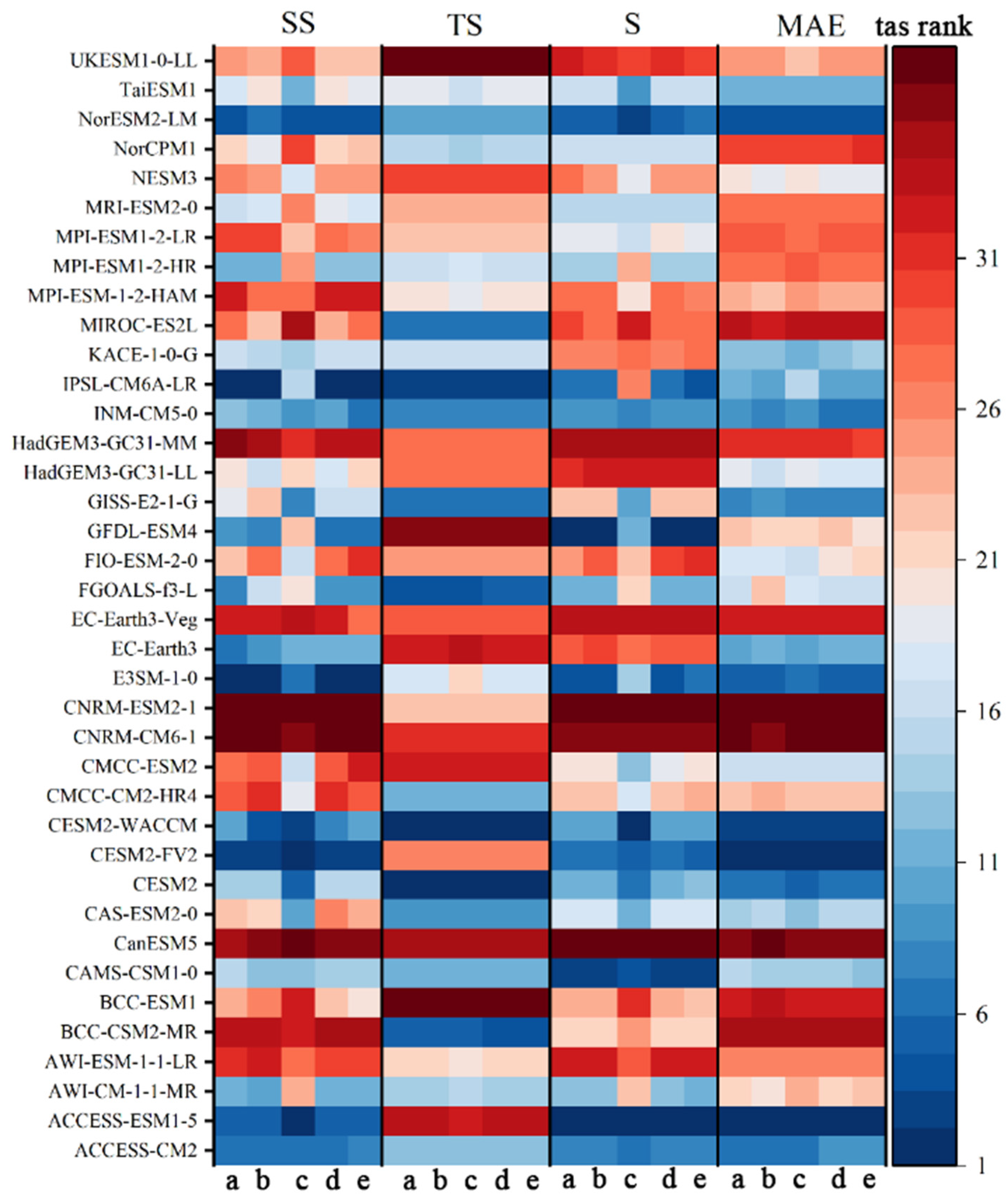
2.3.1. Model Performance Evaluation Indicators

As part of the assessment of model simulation capabilities, we compare the spatial distribution of elements including temperature and precipitation over climate averages and analyze the annual average variability of each model meteorological element over the selected time period.

(1) Mean Absolute Error (MAE)

MAE is the average for the sum of absolute errors between all simulations and corresponding observations, which is better than the average error and effectively prevents errors to offset each other, thus correctly indicating the extent of the overall deviation of the prediction [20]. It can be mathematically written as the following:

$$MAE=\frac{1}{n}{\displaystyle \sum _{i=1}^n|P_i-O_i}|$$

(1)

where P_i is the downscaled or raw value, O_i is the observed value, and n is the number of records of all validated stations.

(2) Time Skills Score (TS)

SS can be used to quantitatively evaluate the effect of individual climate models on the simulation of temporal variability, which measures the difference between the simulated and observed interannual variability of the time series at each image element in the study area as a ratio of standard deviations [21]. It can be mathematically written as the following:

$$TS={\left(\frac{ST{D}_m}{ST{D}_o}-\frac{ST{D}_o}{ST{D}_m}\right)}^2$$

(2)

where $ST{D}_m$, $ST{D}_o$ are the standard deviation values of the time series at each image point in the simulated and observed fields, respectively; according to the evaluation criteria, the closer the value of TS is to 0, the smaller the difference between the standard deviation of the observed and simulated fields is, indicating that the simulation ability of the climate model is better, and vice versa, the worse the simulation performance of the climate model is.

(3) Taylor diagram-based evaluation method (S)

The three indicators, correlation coefficient, standard deviation and central root mean the square error of the combined model and measured series are plotted in polar coordinates as a scatter plot to visually judge the simulation effectiveness of the climate model [22]. In order to quantify the evaluation results of the Taylor diagram, the standard deviation and correlation coefficient of the simulated and observed fields are introduced as the indicator S to further quantitatively evaluate the simulation capability of the climate model. It can be mathematically written as the following:

$$S=\frac{4{(1+R)}^4}{{({\sigma }_f+1/{\sigma }_f)}^2{(1+R_o)}^4}$$

(3)

where R is the correlation coefficient between each climate model and the observed data; R_o is the maximum of the correlation coefficients of all the evaluated objects; and ${\sigma }_f=ST{D}_m/ST{D}_o$, $ST{D}_m$ and $ST{D}_o$ are the standard deviations of the simulated and observed fields, respectively. It can be seen that the more consistent the simulated results are with the observed data, the more S tends to be close to 1, and the better the simulation effect of the climate model.

(4) Spatial Skills Score (SS)

The spatial skill score is used to measure the ability of each climate model to simulate the spatial distribution characteristics of the evaluation variables in the same period, taking into account the spatial mean deviation and correlation coefficient between the simulated and observed fields. It can be mathematically written as the following:

$$SS=1-\frac{MSE(m,o)}{MSE(\overline{o},o)}=r_{m,n}^2-{\left[r_{m,o}^2-(s_m/s_o)\right]}^2-{\left[(\overline{m}-\overline{o}/s_o)\right]}^2$$

(4)

where SS is the dimensionless index; m and o are the data of simulated and observed fields, respectively; $MSE(m,o)$ and $MSE(\overline{o},o)$ denote the mean square error of simulated and observed fields, respectively; $r_{m,o}$ is the correlation coefficient of simulated and observed fields; and $s_m$ and $s_o$ are the mean squared errors of the simulated and observed fields, respectively. It can be seen that the closer the SS is to 1, the better the simulation effect of the climate model.

2.3.2. Spatial Interpolation

In this study, we use 5 different interpolation methods to obtain high-resolution values and compare them. These include Spline, which uses a mathematical function that minimizes the total curvature of the surface to estimate the value, resulting in a smooth surface that passes exactly past the input point [23]. The second method is Kriging, used for when it is required that the spacing and orientation of the scattered points can express the spatial correlation of the surface trend change in the point group [24]. The third method is the Inverse Distance Weighted (IDW), where the inverse of the power of the distance between the predicted point and the sample point is used as the weight of the weighted average [25]. The fourth method is Natural Neighbor Interpolation (NNI), based on the nearest sample subset of the predicted points, where the proportion of the region size is used as the weight of the position of the respective points for interpolation [26]. For the final method, Bilinear Interpolation (BI), linear interpolation is performed on two different directions of the interpolation position, and then the results of the two interpolations are weighted and averaged [27].

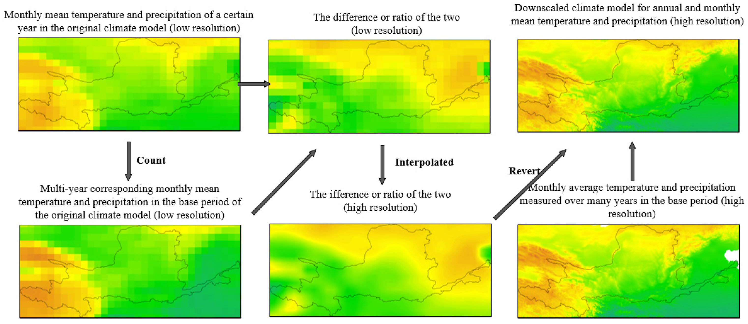
2.3.3. Statistical Downscaling

In this study, observations from 93 ground-based meteorological stations in the YRB area are used as independent variables, while climate model simulations of monthly precipitation and temperature at the corresponding stations are used as dependent variables through the application of Delta downscaling using a spatial raster of multi-year averages of January–December precipitation and temperature with a resolution of 1 km for the base period of 1971–2000. Delta downscaling is a method to obtain future climate scenarios based on the series of measured climate elements in the base period and the characteristic values of variables (e.g., absolute increase in temperature, relative rate of change in precipitation, etc.) of regional future climate models, which are superimposed on each other. This method has the advantage of being relatively simple and less computationally intensive and is capable of downscaling GCM simulations to specific stations. Different downscaling methods are used for different variables. It can be mathematically written as the following:

$$T_f=T_o+(T_{Gf}-T_{Go})$$

(5)

$$P_f=P_o.\frac{P_{Gf}}{P_{Go}}$$

(6)

where T_f is the temperature downscaling data for the prediction period, T_Gf is the simulated temperature data for each grid point in the study area during the prediction period, T_Go is the simulated average temperature data for the grid points in the study area during the base period, T_o is the measured average temperature data for the corresponding grid points during the base period, P_f is the precipitation data after the Delta downscaling, P_Gf is the simulated precipitation data at each grid point in the study area during the predict period, P_Go is the simulated precipitation data at the grid point in the study area during the base period, and P_o is the measured precipitation data at the corresponding grid point during the base period. The specific downscaling process is shown in the figure (Figure 2).

2.4. Space field analysis

The empirical orthogonal function (EOF) is a method for analyzing the structural features in matrix data and extracting the main data feature quantities [28]. When the PCA method was introduced into the analysis of meteorological problems, the meteorological field referred to the method as EOF decomposition. It can be mathematically written as the following:

$$C=X·X^T=(V·T)·{(V·T)}^T=V·\Lambda ·V^n$$

(7)

where V is the spatial eigenvector corresponding to the EOF input variable X, Λ is the diagonal matrix of eigenvalues, and the contribution rate of the corresponding V is calculated based on Λ. T is the time coefficient matrix, which is obtained by multiplying the spatial eigenvector V with the input variable X, and finally decomposing X into the product of the spatial eigenvector and the time coefficient matrix. It can be mathematically written as the following:

$$\begin{array}{l}T=V^T·X\\ X=V·T\end{array}$$

(8)

3. Results

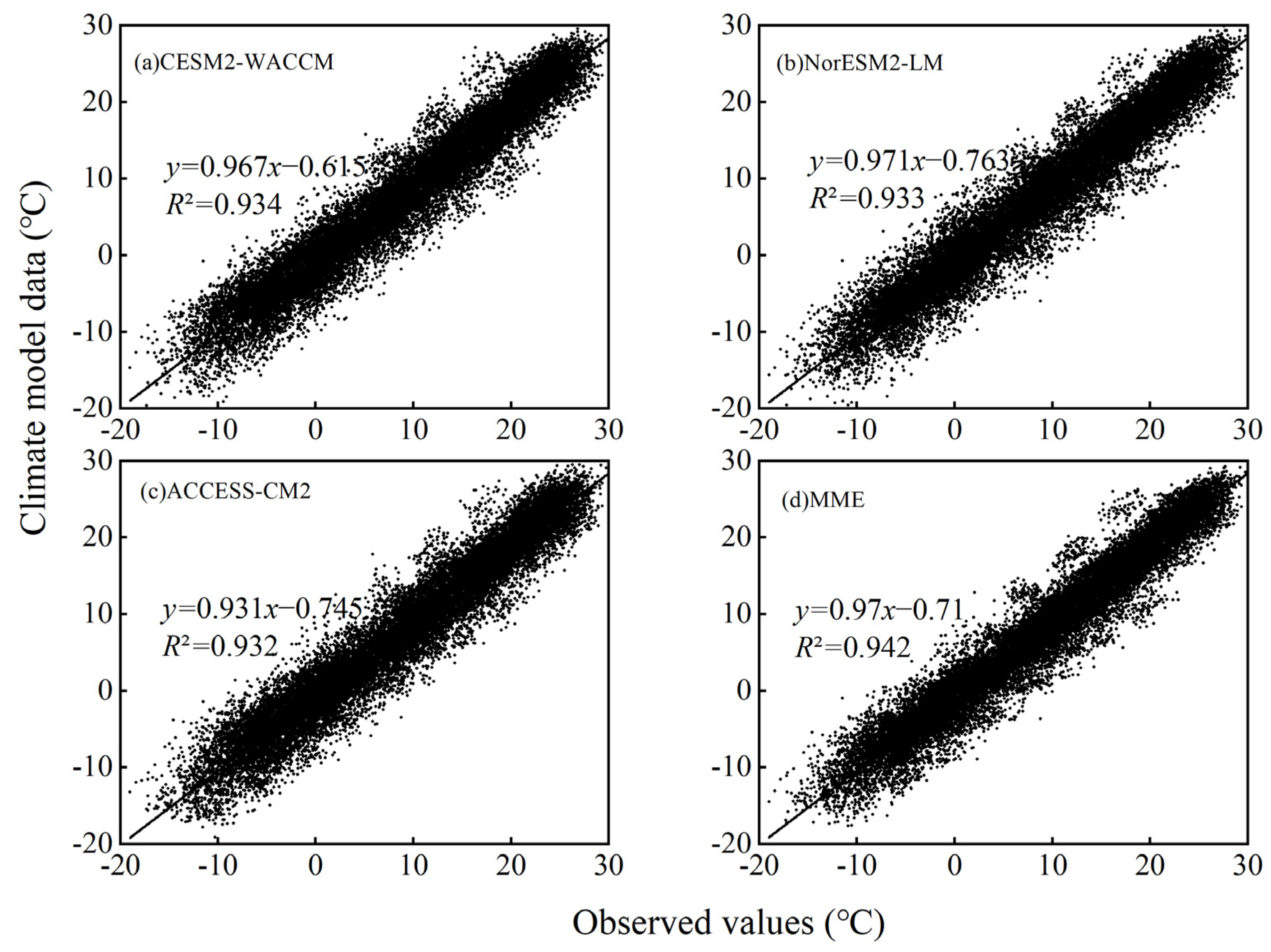
3.1. Downscaling Results Evaluation and Multimodal Ensemble

For temperature, the BI shows minimum error among the four different evaluation indicators, so this interpolation method is used to further evaluate the effect of temperature simulation. The ACCESS-CM2, ACCESS-ESM1-5, CASMS-CSM1-0, CESM2, CESM2-FV, E3SM-1-0, INM-CM-5-0, CanESM5, CESM2-WACCM, FIO-ESM-2-0, INM-CM5-0, NorESM2-LM, etc., rank higher among all climate models for each of the evaluation indicators, with simulated and observed MAE in the range of 23–26 mm, SS in the range of 0.16–0.39, S in the range of 0.82–1, and TS in the range of 0–0.005. It can be seen from the evaluation criteria of the four evaluation indicators that each higher-ranked climate model has a better performance in the temperature simulation performance level of the YRB, indicating that these models can better reflect the temperature characteristics of this region. Considering the data integrity of the climate models and the performance of the actual fits, three climate models, CESM2-WACCM, NorESM2-LM, and ACCESS-CM2, are used to study the future temperature trends in the YRB (Figure 3).

Different from temperature, precipitation using the Kriging can significantly reduce the interpolation error of the climate model. With this interpolation, based on the four different evaluation indicators, the CanESM5, NESM3, CESM2-WACCM, FIO-ESM-2-0, INM-CM5-0, CESM2-WACCM, NorESM2-LM, ACCESS-CM2, ACCESS-ESM1-5, IPSL-CM6A-LR, etc., rank higher among all climate models for each of the evaluation indicators, with simulated and observed MAE in the range of 23–26 mm, SS in the range of 0.16–0.39, S in the range of 0.82–1, and TS in the range of 0–0.005. From the evaluation criteria of the four indicators, the MAE of each of the top-ranked climate models shows no significant difference; due to more spatial sampling points, SS is below 0.5 and far from 1, while both S and TS are close to 1 and 0, respectively, with high performance results, indicating that the model simulates the precipitation characteristics of the Yellow River region to a certain extent and has a high confidence level. Considering the data completeness of the climate model and the performance of the actual fit, three climate models, the ACCESS-ESM1-5, CESM2-WACCM, and IPSL-CM6A-LR, are used for the subsequent analysis of precipitation changes (Figure 4).

For precipitation, the R² of observed and simulated precipitation for the ACCESS-ESM1-5, IPSL-CM6A-LR, and CESM2-WACCM are 0.408, 0.430, and 0.464, respectively, and the regression coefficients are 0.616, 0.624, and 0.644. Overall, the simulated values of the precipitation data are low compared with the observed values, while there are some points with poor fitting. For temperature, the R² for the CESM2-WACCM, NorESM2-LM, and ACCESS-CM2 observed and simulated temperatures are 0.934, 0.933, and 0.932, respectively, and the regression coefficients are 0.967, 0.971, and 0.931, with most points near the 1:1 line. The fit results of the three climate models are similar, and the R² and regression coefficients are greater than 0.9, all passing the 99% confidence level test. The arithmetic mean ensemble of the preferred temperature and precipitation climate models is used to obtain the MME, which performs better than the other single models in the evaluation test, with its MAE dropping to 21.874 mm and both SS and S improving significantly, indicating that MME provides a better fit. The simulated and observed values of the MME dataset are more concentrated than the three independent climate models, which can reduce the errors caused by outliers to a certain extent and improve the fit of the simulated data (Figure 5 and Figure 6).

3.2. Precipitation and Temperature Characteristics of Future Climate Scenarios

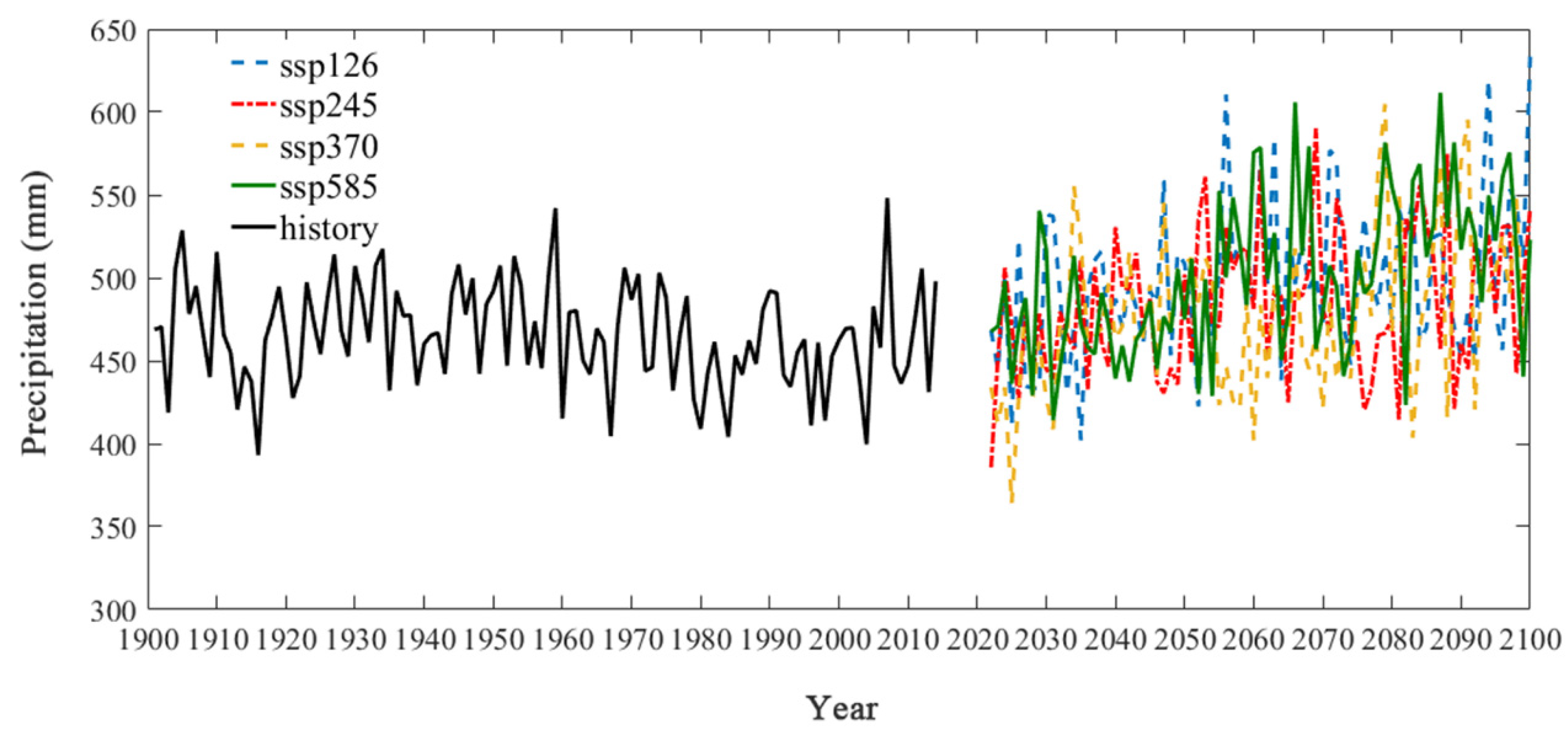
3.2.1. Trends in Precipitation

The multi-year mean precipitation from 1901 to 2014 is 465.78 mm, with a standard deviation of 31.24 mm. The annual precipitation fluctuates widely up and down, with an average variation rate of −1.45 mm/10a. The annual precipitation in different scenarios under the future scenario has similar interannual variation trends, which mainly shows that the fluctuations of precipitation phases in different scenarios are generally consistent, and there is a lagging or early relationship in the appearance of precipitation peaks in some years. In the four ssp126, ssp245, ssp370, and ssp585 scenarios, the increase rates of annual precipitation are 6.89 mm/10a, 5.31 mm/10a, 7.02 mm/10a, and 10.18 mm/10a, respectively. All four scenarios exhibit a strong growing tendency. Overall, there are no discernible changes between the annual precipitation fluctuation trends in the past and the future (Figure 7).

The variance contribution of the EOF1 for different climate scenarios exceeds 50%, which is the main feature of the spatial distribution of precipitation in the YRB for each scenario. The precipitation variability increases from the northwest to southeast, and the eigenvalues of all four EOF1s are positive, indicating a consistent trend in precipitation over the region. For example, the southern region of the EOF2 in the ssp126 and the western part of the EOF3 under various emission scenarios show areas of negative values, indicating that the precipitation in this region is relatively low compared to the multi-year mean precipitation. The two low emission scenarios, ssp126 and ssp245, and the two high emission scenarios, ssp370 and ssp585, show opposite north–south distributions for EOF2, with the former decreasing in the south and increasing in the north while the latter increases in the south and decreases in the north; EOF3 shows the opposite east–west distributions, respectively (Figure 8).

The trend of time coefficients for different EOFs, where a larger absolute value of the time coefficient indicates that the spatial distribution of precipitation in the basin contains a greater proportion of this EOF in this year. PC1 for the ssp126, ssp245, and ssp585 show more negative values until the 2050s and 2060s, indicating a tendency for the whole basin to have less precipitation relative to the multi-year mean precipitation. In contrast, from the 2060s to the end of the century, a more pronounced area of positive values is observed, indicating a basin-wide trend of more precipitation relative to the multi-year mean precipitation. The changes in PC2 and PC3 under different scenarios are more stable, without a relatively obvious trend direction. The years with larger absolute values of EOF indicate that the year exhibits a more pronounced spatial distribution of the mode (same or opposite). For example, the PC2 of the ssp585 indicates a more obvious southeast–northwest distribution of precipitation in the YRB in 2063, 2070, and 2080 (Figure 9).

3.2.2. Trends in Temperature

The multi-year mean temperature from 1901 to 2014 is 6.59 °C, with a standard deviation of 0.59 °C and an average change rate at 0.0038 °C/10a. Similar to precipitation, the annual temperature in the YRB under the four future scenarios shows a more obvious increasing trend compared with the history, and a clear linear tendency. The temperature increase rates under the four scenarios of ssp126, ssp245, ssp370, and ssp585 are 0.1 °C/10a, 0.3 °C/10a, 0.5 °C/10a, and 0.7 °C/10a, respectively, and the temperature increases with the emissions concentration in different scenarios. Under the ssp126 scenario, the average change rate is 0.1 °C/10a, which will exceed 8 °C in 2100. Under the ssp585 scenario, the interannual average change rate of annual temperature is 0.7 °C/10a (p < 0.01), and the R2 exceeds 0.98, indicating a significant increase in annual temperature with a mainly linear tendency, reaching a maximum of 12.87 °C within 100 years in 2100. The ssp245 and ssp370 have the closest temperature trends to the 1980–2014 period (Figure 10).

The EOF1 under all four climate scenarios shows positive region-wide eigenvalues. In the ssp126 scenario, the variance contribution of the EOF1 in the YRB temperature is 82.43%, which plays a major role. The variance contribution of EOF2 is 9.49%, while the contribution of the EOF1 in the other three scenarios is above 95%. The EOF1 eigenvalues of different scenarios are positive, indicating that the basin-wide temperature shows an increasing trend. The EOF1 in the two low emission scenarios shows a relatively obvious east–west distribution, and the positive center of the ssp245 is obviously south compared with the ssp126; the eigenvalues are smaller at the lower reaches of the Yellow River, while the EOF1 in the two high emission scenarios shows a more similar north–south distribution. The spatial trend of the EOF2 of the ssp126 shows a more obvious east–west difference, reflecting a secondary feature of opposite temperature trends in the basin above the XiaHeYan and in the middle and lower reaches (Figure 11).

The PC1 of different scenarios shows a linear increasing trend, and the temperature increases faster with increasing carbon emission concentration from the low emission scenario ssp126 and ssp245 to the high emission scenarios ssp370 and ssp585. Each EOF1 show negative values until the 2050s and 2060s, indicating that the temperature of the YRB is relatively low compared to the multi-year mean temperature, while it is relatively high after the 2060s, with distinctly cooler and warmer periods. In contrast to PC1, the PC2 of ssp126 has no obvious trend and alternates frequently between warm and cold periods (Figure 12).

4. Discussion

4.1. Improvements in Climate Model Preference

The regional terrain, subsoil, and atmospheric conditions—all of which have clear regional characteristics—have a substantial impact on temperature and precipitation. In order to obtain high-resolution grid map data for illustrating the spatio-temporal characteristics of climate change, Shiru et al. (2020) [28] and Tian et al. (2021) [29] applied the direct spatial interpolation of meteorological station data; however, the impact of topographic features on climate change is still not taken into consideration. For the spatial downscaling of the gridded climate dataset, the Delta method with a high spatial resolution reference climate dataset that incorporates topography effects is employed, such that the resulting high spatial resolution gridded map data has accurate geographical location and area information. Consequently, the spatial downscaling dataset obtained in this work comprises topographic features and gives very precise geographical information, such as geographic location, area ratio, and other statistical indicators. Based on this dataset, the results concerning an examination of the spatial distribution characteristics of climate change in the YRB are more trustworthy.

Compared to other studies using Delta spatial downscaling [30], this study obtained lower MAE values for precipitation and temperature downscaling in the ranges of 23–26 mm and 2.1–2.4 °C, indicating the feasibility of downscaling GCM meteorological data to a 1 km × 1 km grid in the YRB using the Delta method. In addition, five interpolation methods are utilized in the downscaling process of this study, which decreases the errors created using the Delta method in the interpolation process and provides more fair and accurate downscaling results. The BI and Kriging are the most applicable interpolation methods for the downscaling of precipitation and temperature in the research area, and they offer promising application possibilities in the climate study of the YRB.

Wang at al. (2021) [30] synthetically evaluated the applicability of 19 climate models to daily precipitation in the YRB by using the rank score (RS) method with eight indicators like the MAE and correlation coefficient, and the results showed that the climate models with better simulation results are in the order of the MRI-ESM2-0, ACCESS-CM2, CNRM-CM6-1, CNRM-ESM2-1, FGOALS-f3-L, and MPI-ESMI-2-HR. Peng et al. (2018) [18] investigated the simulation performance of 28 climate models for climate change in the Loess Plateau region of China and determined that the GFDL-ESM2 and NorESM1 m had the best monthly precipitation and temperature simulation performance. The inconsistency between these conclusions and the paper’s findings is likely owed to the variable evaluation indicators, temporal resolution, and downscaling or lack thereof of the datasets, all of which might influence the evaluation outcomes. This research uses 39 CMIP6 climate models, five spatial interpolations, Delta downscaling, and four separate assessment metrics to analyze the application of watershed precipitation; the conclusions are exhaustive and trustworthy.

In addition to meeting the needs of this study, the Delta method can be used to further downscale the climate data to obtain a higher resolution (30 m × 30 m) for the study of climate trends in the YRB, and these high-resolution climate data can be used as driving data for other fields like hydrological simulation, vegetation succession simulation, crop growth simulation, etc.

4.2. Future Trends of Precipitation and Temperature in the YRB

Numerous studies have indicated that future average precipitation and temperature in China will increase [31], and Zhu et al. (2016) [32] found a similar result for daily rainfall in the YRB between 2015 and 2050 for CMIP5 and CMIP6, with an increase of 0.16 mm/day, and an increase in average temperature of 1.5 °C and 2.2 °C for CMIP5. Guo et al. (2022) [19] demonstrated that, relative to 1971–2000, the annual temperature increased by 1.64–2.20 and 2.31–5.29 °C during the future periods 2026–2055 and 2066–2095, respectively, for CMIP6 and by 1.92–2.39 and 1.68–4.76 °C for CMIP5; in terms of precipitation, CMIP6 increased by 3.45–4.70 and 6.77–15.40%, while CMIP5 increased by 2.58–2.96 and 3.83–9.95%. The results of this study also indicate that different scenarios exhibit significant increases in annual precipitation and temperature relative to 1900–2014, with annual precipitation growth rates of 0.689 mm/a and 1.018 mm/a and temperature growth rates of 0.01 °C/a and 0.07 °C/a for the ssp126 and ssp585 scenarios, respectively. According to these findings, the entire YRB will grow more humid and warmer in the future.

The YRB region of China has a continental monsoon climate with contemporaneous rain and heat, and yearly precipitation is governed mostly by summer precipitation, which is influenced by both the East Asian monsoon and the Indian monsoon [33]. Therefore, the unique properties of each mode can be understood in terms of precipitation formation. On the basis of the EOF1 of precipitation, it is evident that all scenarios exhibit a trend of increasing precipitation across the region, as indicated by consistently higher or lower precipitation across the region, with larger amplitudes in the southeast and smaller amplitudes in the northwest and northeast. The EOF1 of several scenarios demonstrates a constant increase in temperature across the YRB, and all northern regions have higher typical values, which is consistent with the global warming trend process. For the low emission scenarios ssp126 and ssp245, the positive center of the EOF1 is located in the northern portion of the basin; for the high emission scenarios ssp370 and ssp585, it is located in the northern portion of the basin and the Yellow River source region. The second mode EOF2 of ssp126 reflects the secondary feature of the opposite temperature trend in the basin above the XiaHeYan and the middle and lower reaches of the basin, which may be related to the fact that the basin above the XiaHeYan is distributed with mountains and plateaus, having a higher elevation and being more sensitive to temperature fluctuations.

Comparing the predicted and observed data of the CMIP6 downscaled climate model reveals that the simulated values are generally smaller than the observed values and that the simulation performance of different climate models for different climate variables in the same region varies greatly, with a good fit for temperature but a poor fit for precipitation, necessitating the separate verification of the regional applicability under each variable. In addition, it has excellent simulation capabilities for modeling interannual variability, although there is still a discrepancy between its simulated and actual values due to the climate model’s atmospheric physical framework and climate variability.

In general, the applicability of the CMIP6 downscaled climate model over the YRB is higher than that of the CMIP6 unscaled and CMIP5 downscaled climate models, and its uncertainty still needs to be further examined. According to the CMIP6 downscaled climate model, the temperature of the YRB shows a significant increase in the future period, while precipitation mainly shows a significant increase, but with large interannual variability, indicating that the YRB is affected by global warming and tends to be warm and dry, which may exacerbate the water scarcity issue in the YRB. The findings of Kamruzzaman et al. (2021) [34] indicate that the YRB will experience more precipitation during the carbon-neutral period (2015–2060) than during the carbon-peak period (2015–2030), which may mitigate the drought-related disasters caused by global warming-induced increases in evapotranspiration. In light of this, China’s ability to reach carbon neutrality by the end of this century is crucial to resolving the water crisis in the YRB.

5. Conclusions

This study combines different interpolation methods with Delta downscaling to downscale the climate models of monthly temperature and precipitation in the YRB, and verifies their simulation accuracy using four different evaluation indicators; finally, the spatio-temporal characteristics of monthly temperature and precipitation are analyzed according to the MME with the best simulation effect. The Delta downscaling method not only generates more detailed climate information, but also minimizes the uncertainty of the climate model dataset. According to the four indicators, MAE, TS, S and SS, the best fits of each climate model for the monthly mean temperature of the YRB are CESM2-WACCM, NorESM2-LM, and ACCESS-CM2, and the best fits for monthly precipitation are ACCESS-ESM1-5, CESM2-WACCM, and IPSL-CM6A-LR. In general, the MME is superior than the single climate simulation, and the CMIP6 climate model is relatively better for the monthly temperature simulation of the YRB with MME, while the precipitation fitting is poor.

Precipitation and temperature in the YRB during the 21st century are divided into two periods according to the trends, namely, the period of low rainfall and colder temperatures before 2060 and the period of high rainfall and warmer temperatures after 2060. The EOF1 for all scenarios of precipitation indicates a trend of increasing precipitation over the region which is consistent with either high or low rainfall across the region, with larger amplitudes in the southeast and smaller amplitudes in the northwest and northeast. The EOF1 for each scenario of temperature shows a significant rising trend and the warming amplitude grows as the emission concentration rises. The ssp126 and ssp245 regional warming centers are concentrated in the northern portion of the basin, whereas the ssp370 and ssp585 regional warming centers are concentrated in the northern portion of the basin and the Yellow River source region.

The climate model of CMIP6 after Delta downscaling has uncertainties in the simulation of precipitation and temperature in the YRB and performs well in interannual trends, but there are still discrepancies between specific annual numerical simulations and reality. Therefore, in future research, additional downscaling or bias correction methods and alternative high-resolution data sources can be utilized to further minimize the climate model’s uncertainty.

References

1. Omer, A.; Elagib, N.A.; Zhuguo, M.; Saleem, F.; Mohammed, A. Water scarcity in the Yellow River Basin under future climate change and human activities. Sci. Total Environ. 2020, 749, 141446. [Google Scholar] [CrossRef] [PubMed]
2. Li, C.; Kattel, G.R.; Zhang, J.; Shang, Y.; Gnyawali, K.R.; Zhang, F.; Miao, L. Slightly enhanced drought in the Yellow River Basin under future warming scenarios. Atmos. Res. 2022, 280, 106423. [Google Scholar] [CrossRef]
3. Zhou, T.; Zou, L.; Chen, X. Commentary on the Coupled Model Intercomparison Project Phase 6 (CMIP6). Progress. Inquisitiones Mutat. Clim. 2019, 15, 445–456. [Google Scholar]
4. Zhou, S.; Wang, Y.; Chang, J.; Guo, A.; Li, Z. Research on spatio-temporal evolution of drought patterns in the Yellow River Basin. J. Hydraul. Eng. 2019, 50, 1231–1241. [Google Scholar]
5. Fu, Y.H.; Lin, Z.D.; Wang, T. Simulated Relationship between Wintertime ENSO and East Asian Summer Rainfall: From CMIP3 to CMIP6. Adv. Atmos. Sci. 2021, 38, 221–236. [Google Scholar] [CrossRef]
6. Peng, S.Z.; Gang, C.C.; Cao, Y.; Chen, Y.M. Assessment of climate change trends over the Loess Plateau in China from 1901 to 2100. Int. J. Climatol. 2018, 38, 2250–2264. [Google Scholar] [CrossRef]
7. Wang, L.; Li, Y.; Li, M.; Li, L.; Liu, F.; Liu, D.L.; Pulatov, B. Projection of precipitation extremes in China’s mainland based on the statistical downscaled data from 27 GCMs in CMIP6. Atmos. Res. 2022, 280, 106462. [Google Scholar] [CrossRef]
8. Gebrechorkos, S.H.; Hülsmann, S.; Bernhofer, C. Statistically downscaled climate dataset for East Africa. Sci. Data 2019, 6, 31. [Google Scholar] [CrossRef] [PubMed]
9. Liu, C.; Liu, W.; Fu, G.; Ouyang, R. A discussion of some aspects of statistical downscalingin climate impacts assessment. Adv. Water Sci. 2012, 23, 427–437, (In Chinese with English Abstract). [Google Scholar]
10. Storch, H.V. Inconsistencies at the interface of climate impact studies and global climate research. Meteorol. Z. 1992, 4, 72–80. [Google Scholar]
11. Chen, J.; Brissette, F.P.; Leconte, R. Coupling statistical and dynamical methods for spatial downscaling of precipitation. Clim. Chang. 2012, 114, 509–526. [Google Scholar] [CrossRef]
12. Yan, X.; Mohammadian, A. Estimating future daily pan evaporation for Qatar using the Hargreaves model and statistically downscaled global climate model projections under RCP climate change scenarios. Arab. J. Geosci. 2020, 13, 938. [Google Scholar] [CrossRef]
13. Jian, S.; Wang, A.; Su, C. Prediction of future spatial and temporal evolution trends of reference evapotranspiration in the Yellow River Basin, China. Remote Sens. 2022, 14, 5674. [Google Scholar] [CrossRef]
14. Zhang, Z.H.; Deng, S.F.; Zhao, Q.D. Projected glacier meltwater and river run-off changes in the Upper Reach of the Shule River Basin, north-eastern edge of the Tibetan Plateau. Hydrol. Process. 2019, 33, 1059–1074. [Google Scholar] [CrossRef]
15. Hay, L.E.; Wilby, R.; Leavesley, G.H. A comparison of delta change and downscaled GCM scenarios for three mountainous basins in the United States. J. Am. Water Resour. Assoc. 2000, 36, 387–397. [Google Scholar] [CrossRef]
16. Salahi, B.; Poudineh, E. An evaluation of Delta and SDSM Downscaling Models for simulating and forecasting of average wind velocity in Sistan, Iran. Model. Earth Syst. Environ. 2022, 8, 4441–4453. [Google Scholar] [CrossRef]
17. Jian, S.; Wang, A.; Hu, C. Effect of landscape restoration on evapotranspiration and water use in the Yellow River Basin, China. Acta Geophys. 2023, 46, 1542–1546. [Google Scholar] [CrossRef]
18. Peng, S.; Ding, Y.; Wen, Z. Spatiotemporal change and trend analysis of potential evapotranspiration over the Loess Plateau of China during 2011–2100. Agric. For. Meteorol. 2017, 233, 183–194. [Google Scholar] [CrossRef]
19. Guo, Y.; Yu, X.; Xu, Y.; Wang, G.; Xie, J.; Gu, H.A. Comparative assessment of CMIP5 and CMIP6 in hydrological responses of the Yellow River Basin, China. Hydrol. Res. 2022, 53, 867–891. [Google Scholar] [CrossRef]
20. Wang, L.; Chen, W.A. CMIP5 multimodel projection of future temperature; precipitation; and climatological drought in China. Int. J. Climatol. 2014, 34, 2059–2078. [Google Scholar] [CrossRef]
21. Zhu, H.; Jiang, Z.; Li, L. Projection of climate extremes in China; an incremental exercise from CMIP5 to CMIP6. Sci. Bull. 2021, 66, 2528–2537. [Google Scholar] [CrossRef] [PubMed]
22. Saini, A.; Sahu, N.; Duan, W.; Kumar, M.; Avtar, R.; Mishra, M.; Kumar, P.; Pandey, R.; Behera, S. Unraveling Intricacies of Monsoon Attributes in Homogenous Monsoon Regions of India. Front. Earth Sci. 2022, 10, 794634. [Google Scholar] [CrossRef]
23. Yang, L.; Chen, L.D.; Wei, W.; Yu, Y.; Zhang, H.D. Comparison of deep soil moisture in two re-vegetation watersheds in semi-arid regions. J. Hydrol. 2014, 513, 314–321. [Google Scholar] [CrossRef]
24. Zhu, H.; Liu, S.; Jia, S. Problems of the spatial interpolation of physical geographical elements. Geogr. Res. 2004, 23, 425–432. [Google Scholar]
25. Habib, M. Evaluation of DEM interpolation techniques for characterizing terrain roughness. Catena 2021, 198, 105072. [Google Scholar] [CrossRef]
26. Meng, Y.; Duan, K.; Shang, W.; Li, S.; Xing, L.; Shi, P. Analysis on spatiotemporal variations of near-surface air temperature over the Tibetan Plateau from 1961 to 2100 based on CMIP6 models’data. J. Glaciol. Geocryol. 2022, 44, 24–33. [Google Scholar]
27. Sang, Y.; Ren, H.; Shi, X.; Xu, X.; Chen, H. Improvement of Soil Moisture Simulation in Eurasia by the Beijing Climate Center Climate System Model from CMIP5 to CMIP6. Adv. Atmos. Sci. 2021, 38, 237–252. [Google Scholar] [CrossRef]
28. Shiru, M.S.; Chung, E.S.; Shahid, S.; Wang, X.J. Comparison of precipitation projections of CMIP5 and CMIP6 global climate models over Yulin, China. Theor. Appl. Climatol. 2022, 147, 535–548. [Google Scholar] [CrossRef]
29. Tian, J.; Zhang, Z.; Ahmed, Z.; Zhang, L.; Su, B.; Tao, H.; Jiang, T. Projections of precipitation over China based on CMIP6 models. Stoch. Environ. Res. Risk Assess. 2021, 35, 831–848. [Google Scholar] [CrossRef]
30. Wang, Y.; Li, H.; Wang, H.; Sun, B.; Chen, H. Evaluation of CMIP6 model simulations of extreme precipitation in China and comparison with CMIP5. Acta Meteorol. Sin. 2021, 79, 369–386. [Google Scholar]
31. Zhu, H.H.; Jiang, Z.H.; Li, J.; Li, W.; Sun, C.X.; Li, L. Does CMIP6 Inspire More Confidence in Simulating Climate Extremes over China? Adv. Atmos. Sci. 2020, 37, 1119–1132. [Google Scholar] [CrossRef]
32. Zhu, Y.; Lin, Z.; Wang, J.; Zhao, Y.; He, F. Impacts of Climate Changes on Water Resources in Yellow River Basin; China. Procedia Eng. 2016, 154, 687–695. [Google Scholar] [CrossRef]
33. Bagcaci, S.C.; Yucel, I.; Duzenli, E.; Yilmaz, M.T. Intercomparison of the expected change in the temperature and the precipitation retrieved from CMIP6 and CMIP5 climate projections: A Mediterranean hot spot case, Turkey. Atmos. Res. 2021, 256, 105576. [Google Scholar] [CrossRef]
34. Kamruzzaman, M.; Shahid, S.; Islam, A.T.; Hwang, S.; Cho, J.; Zaman, M.A.U.; Ahmed, M.; Rahman, M.M.; Hossain, M.B. Comparison of CMIP6 and CMIP5 model performance in simulating historical precipitation and temperature in Bangladesh: A preliminary study. Theor. Appl. Climatol. 2021, 145, 1385–1406. [Google Scholar] [CrossRef]
Figure 1. Location and DEM of the YRB and 93 meteorological stations distributed across the rectangular region.
Water 16 01441 g001
Figure 2. Delta downscaling process of climate models in the YRB.
Water 16 01441 g002
Figure 3. The fitting performance ranking of the monthly precipitation series in the YRB from 1995 to 2014 measured by stations and simulated using 39 climate models under different interpolation and evaluation indicators (a, b, c, d, and e represent Kriging, IDW, BI, Natural, and Spline, respectively).
Water 16 01441 g003
Figure 4. The fitting performance ranking of the monthly temperature series in the YRB from 1995 to 2014 measured by stations and simulated using 39 climate models under different interpolation and evaluation indicators (a, b, c, d, and e represent Kriging, IDW, BI, Natural, and Spline, respectively).
Water 16 01441 g004
Figure 5. Scatter plots of monthly precipitation (pr) sequences in the YRB from 1995 to 2014 based on Kriging interpolation.
Water 16 01441 g005
Figure 6. Scatter plots of monthly temperature (tas) series in the YRB from 1995 to 2014 under BI interpolation.
Water 16 01441 g006
Figure 7. Changes in annual precipitation in the YRB from the historical period (1901–2014) to the future periods (2023–2100).
Water 16 01441 g007
Figure 8. Changes in annual temperature in the YRB from the historical period (1901–2014) to the future periods (2023–2100).
Water 16 01441 g008
Figure 9. The main modes of EOF of rainfall spatial field in the YRB for 2022–2100 under scenarios ssp126 (a,e,i), ssp245 (b,f,j), ssp370 (d,h,l) and ssp585 (c,g,k); where the EOF1 (2, 3)_pr _ssp126 (contribution %), EOF1 (2, 3)_pr_ssp245 (contribution %), EOF1 (2, 3)_pr_ssp370 (contribution %), EOF1 (2, 3)_pr_ssp585 (contribution %) denote the 1st (2nd, 3rd) mode of rainfall (pr) in ssp126, ssp245, ssp370, ssp585 scenarios, respectively, and the contribution rate of each mode is shown in parentheses.
Water 16 01441 g009
Figure 10. Time coefficients (PC1-PC3) corresponding to the main modes of EOF of the spatial field of precipitation in the YRB from 2022 to 2100 under different scenarios, including ssp126 (ac), ssp245 (df), ssp370 (gi) and ssp585 (jl).
Water 16 01441 g010
Figure 11. The main modes of EOF of the temperature spatial field in the YRB for 2022–2100 under scenarios ssp126 (a,c), ssp245 (e), ssp370 (b) and ssp585 (d); where the EOF1_tas_ssp126 (contribution %), EOF1_tas_ssp245 (contribution %), EOF1_tas_ssp370 (contribution %), EOF1_tas_ssp585 (contribution %) denote the 1st mode of temperature (tas) in ssp126, ssp245, ssp370, and ssp585 scenarios, respectively, and EOF2_tas_ssp126 (% contribution) denotes the 2nd mode of temperature (tas) in ssp126 scenario, and the contribution rate of each mode is shown in parentheses.
Water 16 01441 g011
Figure 12. Time coefficients corresponding to the main modes of EOF of the spatial field of temperature in the YRB from 2022 to 2100 under different scenarios, including ssp126 (a,b), ssp245 (c), ssp370 (d) and ssp585 (e).
Water 16 01441 g012