An Efficient Seepage Element Containing Drainage Pipe

Abstract

Drainage pipes are often positioned downstream of embankments to mitigate pore pressure, thereby reducing the risk of dam failure. Considering that the size of drainage pipes is much smaller than that of embankment dams, directly discretizing the drainage pipes will generate a huge number of elements. Therefore, this paper proposes a seepage element containing drainage pipes. In this element, the permeability of the drainage pipe is taken as the third type of permeable conductivity condition, and it is considered in the energy functional. The governing equations for the steady-state and the transient seepage element containing drainage pipe are derived using the variational principle, and the infiltration matrix, equivalent nodal seepage array, and water storage matrix of the seepage element containing drainage pipe are obtained. In conjunction with the user-defined element module UEL of ABAQUS 2016 software, the established seepage element containing drainage pipe is programmed. The accuracy and efficiency of the proposed seepage element containing drainage pipe are verified through seepage field simulations of three examples. Finally, the influence of the permeable conductivity of drainage pipes on the pressure reduction effect is investigated, providing a reference for the layout of drainage pipes in embankment defense systems.

1. Introduction

Seepage analysis holds crucial significance in civil and hydraulic engineering. The variations of pore pressure in soil can significantly affect the stability of engineering structures, such as slopes [1,2], tunnels [3], and earth-rock dams [4], etc., which are prone to collapse due to the rapid increase of pore water pressure during rainfall or floods. To mitigate the pore water pressure of soil and enhance the safety and stability of engineering, drainage pipes are often installed into embankments, underground structures, and slope engineering [5,6,7]. The diameter of drainage pipes is usually only 7~8 cm, which is several orders of magnitude smaller than the size of engineering structures. When simulating with the finite element method [8] or the finite difference method [9], it is necessary to divide the relevant areas of drainage pipes into dense mesh to capture the outflow conditions through the pipe wall. However, this will lead to a significantly large and time-consuming calculation scale, which is even more challenging to perform. Therefore, it is very important to adopt a reasonable method for the efficient simulation calculation of drainage pipes.

In the early calculations, the “points instead of holes” method was utilized [10], treating drainage holes as given head nodes. Due to the significant head gradient near the drainage holes in this method, when simulating with the aforementioned approach, the mesh division must be sufficiently fine; otherwise, the role of drainage holes will be excessively magnified. Fipps [11] suggests that when employing the “points instead of holes” method, substituting a given flow rate for the given head will significantly weaken the impact of mesh partitioning accuracy on calculation results. Subsequently, more and more research has improved the simulation of drainage pipes, and some effective methods have emerged to simulate the functions of drainage pipes, such as the rod element method [12], the convergence element method [13], the drainage substructure method [14], the improved drainage substructure method [15,16,17], the line-substitution hole method [18], the sandwich instead of holes array method [19], the air element method [20], the composite element method [21,22,23,24,25], etc.

The rod element method [12] essentially achieves drainage by simulating the flow rate of drainage pipes. This method has simple programming and low computational complexity, and it can indeed reflect the drainage effect to a certain extent. However, this method only simulates the drainage volume of drainage pipes at a macro level, making it difficult to ensure accuracy. Therefore, based on the rod element, Wang [13] proposed the convergence element method, which is an improvement on the rod element. From the perspective of groundwater movement, the drainage well is regarded as a convergence line and embedded into the conventional finite element to establish a convergence line element. Compared with the rod element method, this approach takes into account the influence of aquifer thickness on flow rate, resulting in a significant improvement in calculation accuracy and clearer physical concepts. However, when the flow around the well is not radial, this method may introduce significant calculation errors.

To further improve computational accuracy, Wang proposed the drainage substructure method [14]. This method treats the drainage pipe and the surrounding soil or rock within a certain range as a substructure and eliminates the internal degrees of freedom of the substructure through condensation. Only the degrees of freedom on the common boundary between the adjacent structures, as well as on the constraint boundary, need to be considered. The drainage substructure method basically addresses the problem of seepage fields when the drainage hole does not pass through the seepage-free surface. However, when a drainage pipe passes through the free surface, there will be seepage of virtual domains and virtual elements inside the drainage substructure, resulting in significant errors. To avoid the errors brought about by the drainage substructure method in specific situations, many scholars have made improvements on the basis of this method. This paper summarizes this type of method as the improved drainage substructure method. Chen [15] proposed a method that combines the drainage substructure method, Signorini’s type variational inequality, and the adaptive penalty Heaviside function (SVA) to solve the seepage problems of dam sections with drainage pipes. The study concluded that a pipe spacing of 10 m is suitable for the arrangement of drainage pipes. Xu [16] proposed a new simulation method for the drainage hole array and conducted a seepage control analysis for the Qingyuan Pumped Storage Power Station. This method simplifies the drainage hole with a diameter of 5 cm into a line element and ignores the size of the drainage hole. Compared with the substructure method, this method uses fewer nodes and elements in simulating complex hole arrays, making the modeling simpler. However, for drainage hole arrays with larger diameters, this method needs to be improved. Su [17], in combination with the nodal virtual flow method, also proposed an improved drainage substructure method. This method arranges large parent elements according to the direction of the drainage holes during the finite element mesh division and divides the parent elements that pass through the drainage holes into sub-elements to form substructures. By applying the condensation of internal degrees of freedom and boundary conditions to the substructures, it reduces the difficulty of finite element mesh division and the computational amount of solving equations.

Bai [18] conducted a seepage control analysis for the Heihe Reservoir and proposed “the line-substitution hole method“. This method reflects the drainage hole as a one-dimensional line element with strong permeability performance in the permeable medium structure and leaves traces on the corresponding volume through the Boolean operation function of ADINA. This method does not consider the specific size of the drainage hole, reducing the modeling workload and effectively improving the modeling efficiency of complex anti-seepage systems. When there are a large number of drainage pipes forming a well array, Zhu [19] proposed the sandwich instead of the hole array method, which replaces the drainage hole array with an equivalent drainage interlayer. In this method, the horizontal permeability coefficient of the interlayer matches that of the rock foundation, while the vertical permeability coefficient is judiciously chosen to achieve similar drainage effects. The seepage field calculated by the sandwich instead of the hole array method has almost identical mechanical effects compared to the seepage field calculated based on actual drainage holes. And the calculation of the mesh remains is not affected by the radius and spacing of the drainage holes, resulting in a great simplification. However, due to the impact of equivalence, there is a slight compromise in accuracy.

When a project contains a large number of drainage holes, it is difficult to analyze each drainage substructure. Therefore, Hu [20] proposed the air element method, which is similar to the line-substitution hole method. This method treats the drainage holes as elements filled with air as the seepage medium. After assigning the corresponding permeability coefficient, it incorporates them into the traditional finite element seepage calculation method, just like regular elements. This method does not require the boundary head of the drainage holes to be given, reducing the data preparation workload. However, to obtain accurate calculation results, it is necessary to encrypt the mesh near the drainage holes. When there are many drainage holes, the computational workload is quite large.

With the continuous deepening of research on simulation methods for drainage holes, Chen proposed the composite element method [21,22,23,24,25] based on the air element. This method employs a composite element for seepage analysis of drainage holes, treating them as strong permeable mediums and embedding them as “air subelements” within conventional geotechnical elements, forming composite elements that cover the drainage holes. The composite element method can accurately simulate the role of each drainage hole and avoid the difficulty of mesh generation for drainage holes. However, this method does not distinguish the influence of seepage state on drainage holes and is not suitable for transient seepage.

The above methods can be summarized into two categories: one is to seek a macro-equivalent approach to avoid the direct physical simulation of drainage holes, as long as the “drainage effect” is simulated, such as the rod element method, the convergence element method, the line-substitution hole method, and the sandwich with hole array method. Although this approach minimally increases the computational workload, the precision is constrained by the “equivalence”, leading to a reduction in calculation accuracy. Another type is to directly simulate drainage holes in the physical domain, such as the drainage substructure method, the improved drainage substructure method, the air element method, and the composite element method. These methods offer higher computational accuracy and can reflect the actual seepage field near the drainage holes. However, when using these methods to simulate drainage pipes in the seepage region, computational amount reduction is achieved through certain assumptions, limiting the applicability of these methods. Consequently, it is necessary to construct efficient and fine element containing drainage pipes for the simulation of the seepage problem.

In this paper, based on the finite element theory of seepage, the third type of permeable conductivity condition for the drainage pipe wall is included in the control equation by the variational principle, and a seepage element for analyzing the drainage pipe effect will be established. The method directly reflects the seepage pressure release and water flow exchange mechanisms of the drainage pipe into the seepage matrix, equivalent to the nodal seepage load array of the element, so that high accuracy can be achieved in the drainage pipe region without the need for mesh subdivision, avoiding the generation of a huge number of elements and improving computational efficiency.

The paper is structured into five sections. Section 2 presents the theoretical basis and calculation model for the element containing drainage pipe in the seepage field. Section 3 describes the UEL subroutine in Abaqus for seepage elements with drainage pipes in the seepage field. Section 4 validates the reliability, efficiency, and accuracy of the element containing drainage pipe by comparing the computational results of the method presented in this paper with those of the line-substitution hole method and explores the pressure reduction effect of permeable conductivity on the seepage area through three examples. Finally, the main conclusions are summarized in Section 5.

2. Theory Presentation and Model Evaluation

2.1. Finite Element Governing Equations of the Seepage Field

According to Darcy’s law [26] and the seepage continuity equation [27], the basic equation of seepage is derived as follows:

$$\frac{\partial \theta }{\partial t}=\nabla \left(k\left(\theta \right)\nabla h\right)$$

(1)

where $h$ is the total water head, which is composed of the positional water head y reflecting the gravitational potential, and the matrix potential head y₀, i.e., h = y + y₀. $\mathit{k}\left(\theta \right)$ is the permeability matrix, and θ is a function of volumetric moisture content.

For saturated soils, the water content remains constant over time as the soil pores are fully saturated, resulting in $\partial \theta /\partial t=0$. This leads to the controlling equation for the movement of water in saturated soils as follows:

$$\nabla \left(k\nabla h\right)=0$$

(2)

where the permeability coefficient $\mathit{k}$ is constant. When accounting for the compression of soil and water, the above equation becomes an unsteady seepage equation, i.e.,

$$\nabla \left(k\nabla h\right)=s\frac{\partial h}{\partial t}$$

(3)

where $s$ is a specific storage coefficient and t is time.

The definite solution conditions of the unsteady seepage field are as follows:

$$\mathrm{Initial} \mathrm{condition}: \begin{array}{c}h{\mid }_{t=0}=h\left(x,0\right)\end{array}$$

(4)

boundary condition:

$$\mathrm{Category} \mathrm{I} \mathrm{boundary} (\mathrm{head} \mathrm{boundary}): \begin{array}{c}h\mid {\Gamma }_1=h\left(x,t\right)\end{array}$$

(5)

$$\mathrm{Category} \mathrm{II} \mathrm{boundary} (\mathrm{flow} \mathrm{boundary}): \begin{array}{c}{k}_n\frac{\partial h}{\partial n}\mid {\Gamma }_2=\overline{q}\left(h,x,t\right)\end{array}$$

(6)

$$\mathrm{Category} \mathrm{III} \mathrm{boundary} (\mathrm{Mixed} \mathrm{boundary}): \begin{array}{c}\left(q_n\right)=\beta \left(h-h_a\right)\end{array}$$

(7)

where $n$ is the normal direction to the outer boundary, $\beta$. The water flow exchange coefficient in this paper is the hydraulic conductivity coefficient of the drainage pipe.

According to the variational principle [28], for a seepage field that meets the first type of boundary conditions, the solution of Equation (2) equates to finding the extreme value of the following generalized function.

$$\begin{array}{c}I\left(h\right)={\displaystyle {\int }_{\Omega }\frac{1}{2}\nabla h^{T}k\nabla h}d\Omega +{\displaystyle {\int }_{{\Gamma }_2}\overline{q}}hds\end{array}+{\displaystyle {\int }_{{\Gamma }_3}\beta \left(\frac{1}{2}{h}^2-h_{\alpha }\right)ds}$$

(8)

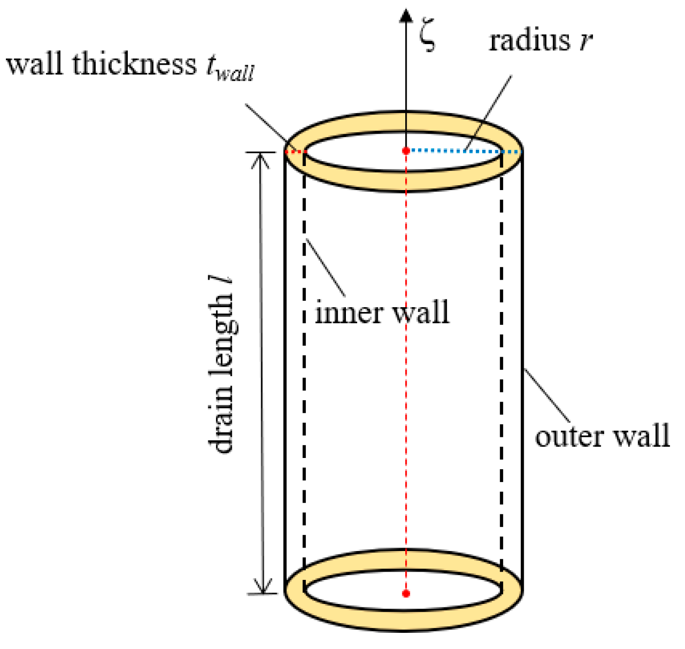
2.2. The Construction of the Seepage Element Containing Drainage Pipe

Consider a typical conventional finite element containing drainage pipe, as shown in Figure 1. The permeability of drainage pipes is much higher than that of soil, so the drainage pipe in element can be taken as the third type of water conducting boundary condition. When the water seeps into the drainage pipes, the seepage pressure is completely released. The hydraulic conductivity domain, that is, the drainage pipe, is denoted as $S_3$. Due to the water flow exchange and the difference between internal and external water heads on the surface of $S_3$, it can be treated as a mixed boundary condition, as shown in Equation (7).

Assuming that the infiltration zone is well consolidated, according to the structural characteristics of the calculation region, it is discretized into a finite element mesh, and the head interpolation function of a certain element is as follows:

$$\begin{array}{l}h\left(x,t\right)=N^{\mathrm{T}}{h}^e\hfill \end{array}$$

(9)

where $N$ is the shape function array of the element and $h^e$ is the nodal head array of the element. There is also a one-dimensional local coordinate $\zeta \left(-1\le \zeta \le 1\right)$ along the direction of the drainage pipe, as shown in Figure 2.

For any a element containing drainage pipe, its total energy functional for a steady seepage state is given as follows:

$$\begin{array}{l}{\Pi }_e=\frac{1}{2}{\left(h^e\right)}^{\mathrm{T}}{\displaystyle {\int }_{{\Omega }_e}\nabla N^{T}k\nabla N}d\Omega \left(h^e\right)+{\left(h^e\right)}^{\mathrm{T}}{\displaystyle {\int }_{S_2^{\mathrm{e}}}{N}^{\mathrm{T}}}\overline{q}ds\hfill \\ \hspace{1em}+\frac{1}{2}{\left(h^e\right)}^{\mathrm{T}}{\displaystyle {\int }_{{\Gamma }_3^e}\beta }{N}^{\mathrm{T}}Nds\left(h^e\right)-{\left(h^e\right)}^{\mathrm{T}}{\displaystyle {\int }_{{\Gamma }_3^e}\beta h_{\alpha }{N}^{\mathrm{T}}ds}\hfill \end{array}$$

(10)

where $h_{\alpha }$ is the water head in the drainage pipe, $\beta$ is the hydraulic conductivity coefficient of drainage pipe, defined as $\beta =k_P/t_{wall}$ with $k_P$ being the permeability coefficient of the drainage pipe, and $t_{wall}$ is the wall thickness of drainage pipe. When neglecting the thickness of the drainage pipe, the hydraulic conductivity of the drainage pipe is treated as the first type boundary condition, that is, the hydraulic conductivity $\beta$ approximates infinity.

Taking the variational derivative of Equation (10) and setting it equal to zero, the steady seepage equations for the element containing drainage pipe can be obtained as follows:

$$\begin{array}{l}\left(P^e+M^e\right)h^e=F^e\hfill \end{array}$$

(11)

where $P^e$ is the elemental seepage matrix contributed by the medium, $M^e$ is the elemental seepage matrix contributed by the drainage pipe, and $F^e$ is the elemental seepage load array. They are as follows:

$$\begin{array}{l}{P}^e={\displaystyle {\int }_{\Omega e}\nabla N^{T}k\nabla N}d\Omega \hfill \end{array}$$

(12)

$$\begin{array}{l}{F}^e={\displaystyle {\int }_{{\Gamma }_3^e}\beta }{h}_{\alpha }{N}^{T}ds-{\displaystyle {\int }_{{\Gamma }_2^e}{N}^T}\overline{q}ds\hfill \end{array}$$

(13)

$$\begin{array}{l}{M}^e={\displaystyle {\int }_{{\Gamma }_3^e}\beta }{N}^{\mathrm{T}}Nds\hfill \end{array}$$

(14)

Due to the small diameter of the drainage pipe, the head and other integrated functions are taken as constants along the circumferential direction of the drainage pipe. The integration over the contact surface of the drainage pipe can be transformed into a one-dimensional integration along its length. Equations (13) and (14) can be reformulated as follows:

$$\begin{array}{l}{F}^e={\displaystyle {\int }_{{\Gamma }_3^e}\beta }{h}_{\alpha }{N}^{\mathrm{T}}ds-{\displaystyle {\int }_{{\Gamma }_2^e}{N}^{\mathrm{T}}}\overline{q}ds=2\pi a\beta {\displaystyle {\int }_{-1}^1{h}_{\alpha }{N}^{\mathrm{T}}\frac{l}{2}d\xi }-{\displaystyle {\int }_{{\Gamma }_2^e}{N}^{\mathrm{T}}}\overline{q}ds\hfill \end{array}$$

(15)

$$\begin{array}{l}{M}^e={\displaystyle {\int }_{{\Gamma }_3^e}\beta }{N}^{\mathrm{T}}Nds=2\pi a\beta {\displaystyle {\int }_{-1}^1{N}^{\mathrm{T}}}N\frac{l}{2}d\xi \hfill \end{array}$$

(16)

where a is the radius of the drainage pipe and $l$ is the length of the drainage pipe in the element.

For an unsteady seepage field, Equation (8) can be changed as follows:

$$\begin{array}{c}I\left(h\right)={\displaystyle {\int }_{\Omega }\left\{\frac{1}{2}\nabla h^{T}k\nabla h+\right.}\left.sh\frac{\partial h}{\partial t}\right\}\mathrm{d}\Omega +{\displaystyle {\int }_{{\Gamma }_2}\overline{q}}hds\end{array}+{\displaystyle {\int }_{{\Gamma }_3}\beta \left(\frac{1}{2}{h}^2-h_{\alpha }\right)ds}$$

(17)

For any a element containing drainage pipe, its total energy functional for an unsteady seepage state is given as follows:

$$\begin{array}{l}{\Pi }_e=\frac{1}{2}{\left(h^e\right)}^T{\displaystyle {\int }_{{\Omega }^e}\nabla N^{T}k\nabla N}d\Omega h^e+{\left(h^e\right)}^T{\displaystyle {\int }_{{\Gamma }_2^e}{N}^T}\overline{q}ds+{\left(h^e\right)}^T{\displaystyle {\int }_{{\Omega }^e}s}{N}^{T}Nd\Omega \left({\dot{h}}^e\right)\hfill \\ \hspace{1em}+\frac{1}{2}{\left(h^e\right)}^T{\displaystyle {\int }_{{\Gamma }_3^e}\beta }{N}^{T}Nds\left(h^e\right)-{\left(h^e\right)}^T{\displaystyle {\int }_{{\Gamma }_3^e}\beta }{h}_{\alpha }{N}^{T}ds\hfill \end{array}$$

(18)

Similarly, taking the variational derivative of Equation (18) and setting it equal to zero, the unsteady seepage equations for the element containing drainage pipe can be derived as follows:

$$S^e{\dot{h}}^e+\left(P^e+M^e\right)h^e=F^e$$

(19)

where $S^e$ is the water storage matrix of element, expressed as follows:

$$S^e={\displaystyle {\int }_{{\Omega }^e}s}{N}^{T}Nd\Omega$$

(20)

For analytical convenience, let $P^e+M^e={\mathit{K}}^e$, then Equations (11) and (19) can be rewritten as, respectively:

$$K^e{h}^e=F^e$$

(21)

$$S^e{\dot{h}}^e+K^e{h}^e=F^e$$

(22)

where ${\mathit{K}}^e$ is the elemental seepage matrix contributed by the medium and drainage pipe.

2.3. Transient Equation Solving Scheme

Due to the fact that transient seepage [29] involves the problem of water heads changing over time, it is not possible to directly solve a system of linear algebraic equations like solving steady-state seepage [30]. For the transient seepage equation, it is expressed as a set of ordinary differential linear algebraic equations with time t as the variable. There are usually two methods for solving this system of equations in finite element analysis: the difference method [31] and the modal superposition method [32]. In this paper, the backward difference method [33] is employed to solve Equation (22), where the solution at temporal nodes is iteratively calculated starting from initial conditions and the nodal head at any moment can be obtained through interpolation.

In the [t, t + Δt] time step, the head change rate $\dot{h}\left(t\right)$ can be expressed as follows:

$$\begin{array}{c}\dot{h}=\frac{\Delta h^e}{\Delta t}=\frac{h_{t+\Delta t}^e-h_t^e}{\Delta t}\end{array}$$

(23)

Substituting Equation (23) into Equation (19), the governing equation at time t + Δt can be expressed as follows:

$$\left(K_{t+\Delta t}^e+\frac{S_{t+\Delta t}^e}{\Delta t}\right)h_{t+\Delta t}^e=F_{t+\Delta t}^e+\frac{S_{t+\Delta t}^e}{\Delta t}{h}_t^e$$

(24)

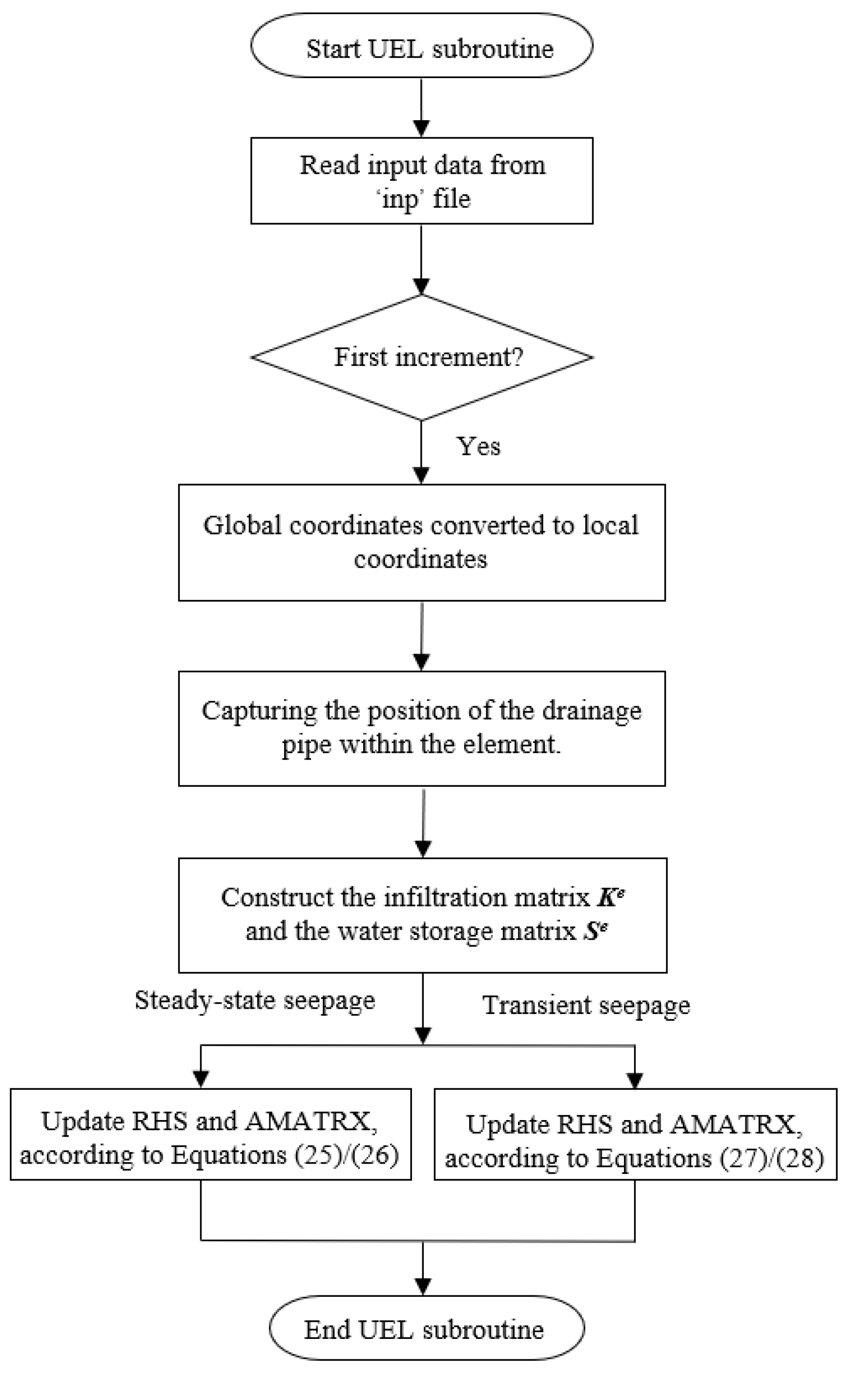
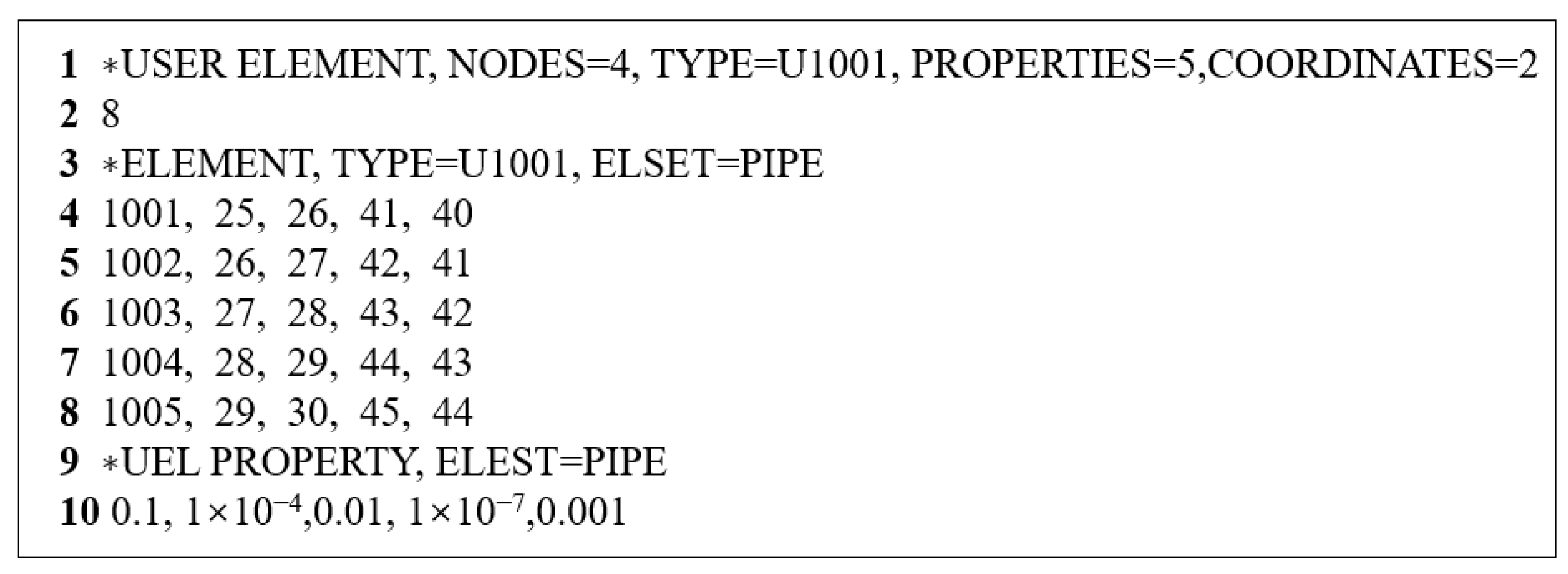
3. Implementation of the Seepage Element Containing Drainage Pipe in Abaqus

Abaqus provides a programming interface called UEL for customizing user elements [34]. Through the UEL subroutine framework, the seepage element containing drainage pipe can be easily developed, and with the powerful solving function, the pre- and post-processing capabilities of Abaqus software can be utilized directly. Moreover, the assembly of element matrices and arrays does not require self-programming. Therefore, the scheme of the user element subroutine UEL for the seepage element containing drainage pipe is adopted in this article.

The UEL framework for user subroutine is shown in Figure 3, which provides the parameters or variables connecting the Abaqus solving process.

In the UEL subroutine framework, RHS denotes the contribution of the element to the residual vector of the overall system of equations, and AMATRX denotes the contribution of the element to the Jacobian (stiffness) or other matrix of the overall system of equations. Therefore, for steady seepage analysis, AMATRX can be used to store the elemental seepage matrix ${\mathit{K}}^e$ contributed by the medium and drainage pipe, and RHS is used to store the elemental seepage load array $F^e$, that is, as follows:

$$AMATRX=K^e$$

(25)

$$RHS=-K^e{h}^e$$

(26)

While, for transient seepage analysis, AMATRX and RHS are stored as follows:

$$AMATRX=K_{t+\Delta t}^e+\frac{S_{t+\Delta t}^e}{\Delta t}$$

(27)

$$RHS=-K_{t+\Delta t}^e{h}_{t+\Delta t}^e-\frac{S_{t+\Delta t}^e}{\Delta t}\left(h_{t+\Delta t}^e-h_t^e\right)$$

(28)

Figure 4 shows a flow chart of the UEL subroutine for the element containing drainage pipe. Based on the input file’s connectivity information, the UEL subroutine converts global coordinates to local coordinates using the given shape function relationships and then automatically searches for the position of the drainage pipe using an inverse transformation algorithm, thereby calculating the length of the drainage pipe inside each element. Subsequently, it constructs the infiltration matrix ${\mathit{K}}^e$ and the water storage matrix ${\mathit{S}}^e$ using Equations (12)–(16). Finally, for different seepage states, it constructs the AMATRX matrix and the RHS matrix using Equations (25)–(28).

PROPS is a floating point array containing the NPROPS real property values defined for use with this element. In the user-defined seepage element containing drainage pipe program, there are 5 properties that need to be provided, which are

PROPS(1): radius $a$ of the drainage pipe;

PROPS(2): permeability coefficient $k_p$ of the drainage pipe material;

PROPS(3): thickness $m_p$ of the drainage pipe;

PROPS(4): permeability coefficient $k$ of the medium;

PROPS(5): specific storage coefficient $s$ of the medium.

U is the array of the nodal water head of the element; for steady seepage analysis, $U=h_t^e$; and for transient seepage analysis, $U=h_{t+\Delta t}^e$.

DU is the incremental value of the water head for the current increment, that is $DU=h_{t+\Delta t}^e-h_t^e$.

TIME(1) is the current value of step time.

TIME(2) is the current value of total time.

DTIME is the time increment.

LFLAGS is an array containing the flags that define the current solution procedure and requirements for element calculations; LFLAGS(1) defines the procedure type; LFLAGS(1) = 62 or 63 for steady analysis; and LFLAGS(1) = 64 or 65 for transient analysis.

By using the UEL program for the seepage element containing draining pipe, the seepage stiffness and residual contribution of the element to the system can be obtained. The Abaqus solver can be called with the following command: abaqus job=<inp file name >user=<fortran file name>.

In the inp file, it is necessary to provide a declaration of the user element and information about all user elements, including the node connection, material properties, and drainage pipe parameters. Taking two-dimensional problems as an example, the parts involving user elements in the inp file are as shown in Figure 5.

Line 1: Declares a user element with 4 nodes and 5 properties, and there are 2 coordinates at each node of the element.

Line 2: An indicator number 8 is given, indicating that the degree of freedom is the pore pressure or the total water head. In this article, the total water head is used.

Line 3: Defines user elements and categorizes them into one set.

Lines 4~8: Lists the element ID and corresponding node connection information of each user element.

Line 9: Assigns the 5 properties to the user elements.

Line 10: Gives the values of the 5 properties: radius of the drainage pipe a = 0.1 m, permeability coefficient of the drainage pipe k_p = 1 × 10⁻⁴ m/s, thickness of the drainage pipe m_p = 0.01 m, permeability coefficient of the medium k = 1 × 10⁻⁷ m/s, specific storage coefficient of the medium s = 0.001 m⁻¹, respectively.

4. Validation and Analysis

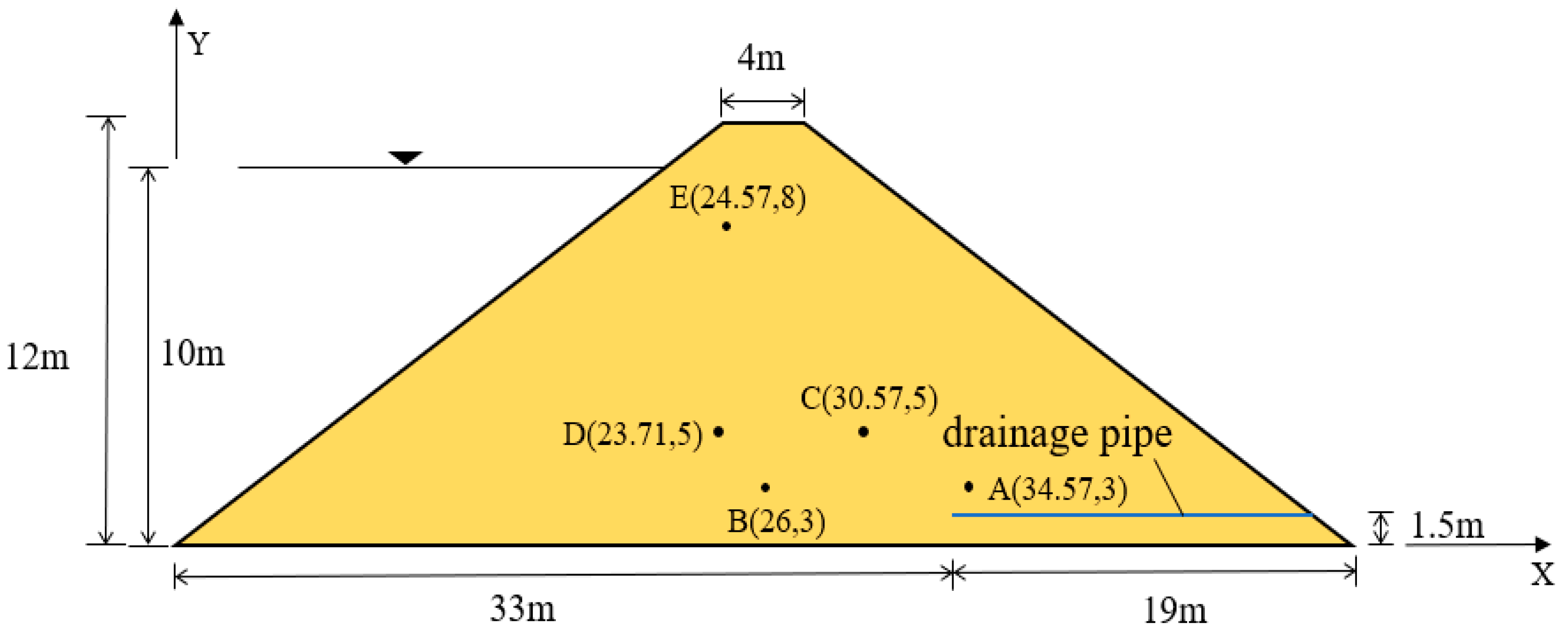
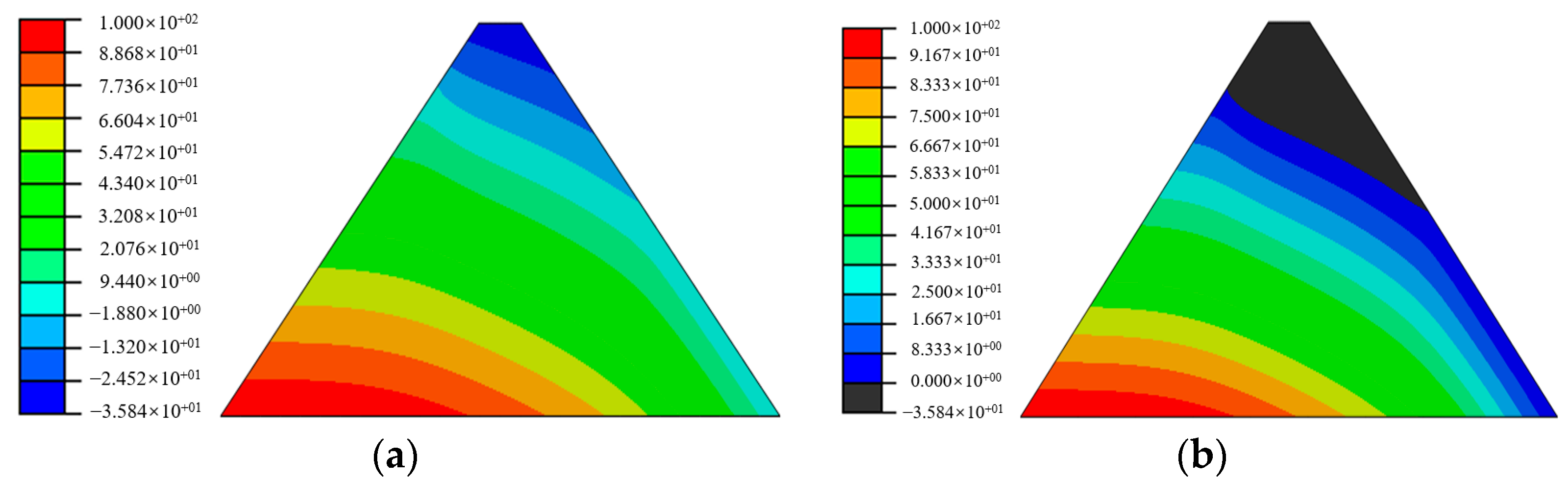
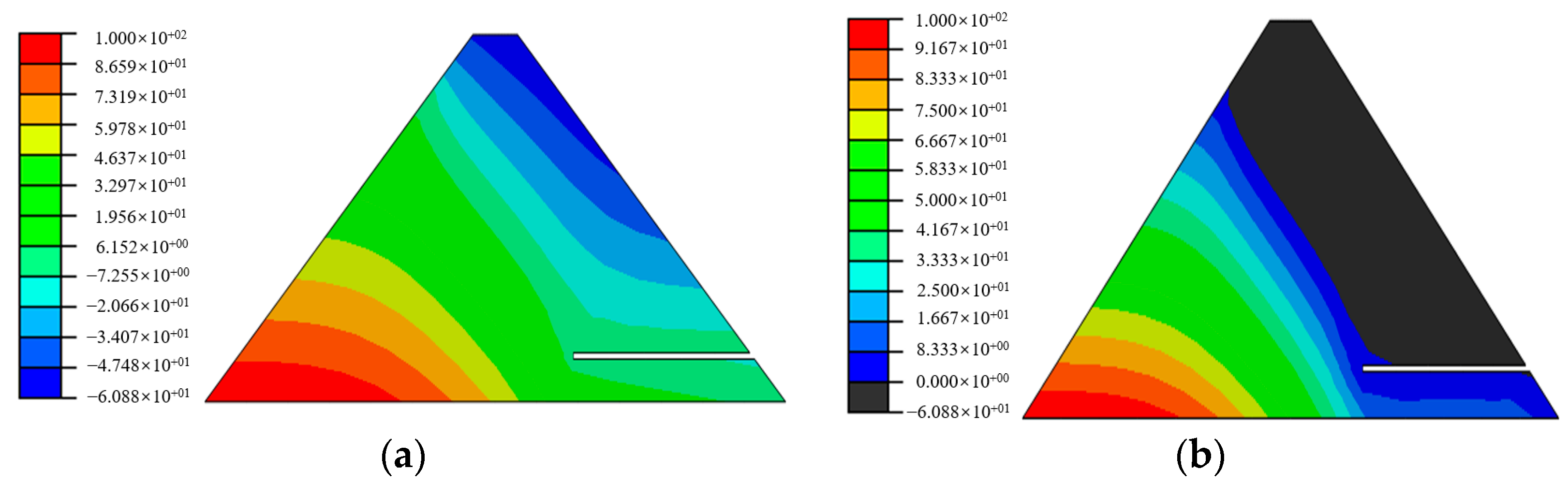
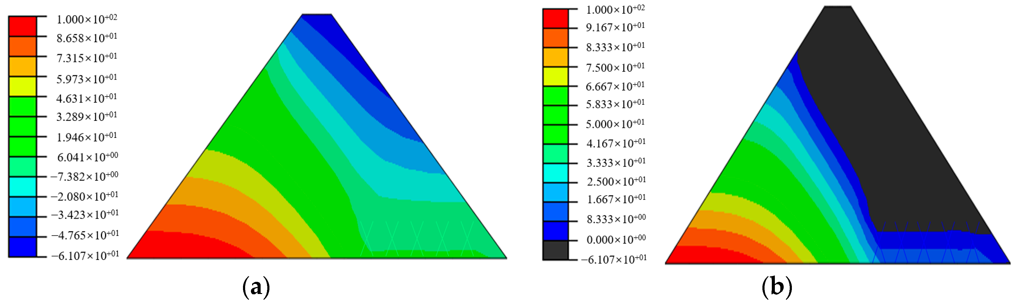
4.1. Steady Seepage Simulation with a New Element Containing Drainage Pipe for a Dyke Dam

A homogeneous dyke dam with a height of 12.0 m, a top width of 4.0 m, a bottom width of 52.0 m, and a slope ratio of 1:2 for both upstream and downstream was used. The upstream water level is 10.0 m higher than the reference surface, and the downstream water level is level with the reference surface. The saturated permeability coefficient of the soil is k = 1.0 × 10⁻⁷ m/s, and the dam bottom is an impermeable layer. Downstream of the dyke dam, a drainage pipe with a length of 16.0 m, a radius of 0.1 m, and a wall thickness of 0.01 m is horizontally buried 1.5 m from the dam bottom, as shown in Figure 6. To verify the effectiveness and reliability of the proposed element in this article, a new element model and a traditional finite element model were used for simulation. The permeability coefficient of the drainage pipe was taken as k_p = 1 × 10⁻⁴ m/s, and the pore pressure distributions and corresponding infiltration surfaces with no grain pipe and a single drainage pipe are shown in Figure 7, Figure 8 and Figure 9, respectively. From the comparison of the results in Figure 7, Figure 8 and Figure 9, it can be seen that the pore pressure distribution of the new element model is very close to those of the traditional finite element method, and the infiltration surface rapidly decreases above the drainage pipe, reflecting the significant pressure reduction effect of the drainage pipe verifying the reliability and effectiveness of the new seepage element containing drainage pipe.

To further investigate the pressure-reducing capability of drainage pipes, the pressures at monitoring points A, B, C, D and E in the dam body are investigated for three scenarios: no drainage pipe layout, drainage pipe with permeability coefficient k_p = 1 × 10⁻⁴ m/s, and drainage pipe with permeability coefficient k_p = 1 × 10⁻⁶ m/s. The pore pressures of the three scenarios at monitoring points are listed in

Table 1. Pore pressures at monitoring points (kPa).

Method	Case	Monitoring Points
		A	B	C	D	E
Traditional FEM	No drainage pipe layout	38.5672	54.5833	27.2837	38.5764	7.9902
	With kp = 1 × 10−4 m/s	−8.5477	28.9266	−9.0734	19.9254	−11.1304
	With kp = 1 × 10−6 m/s	−8.5313	28.9302	−9.0672	19.9282	−11.1271
UEL	With kp = 1 × 10−4 m/s	−9.0211	28.1991	−9.5175	19.5152	−11.4228
	With kp = 1 × 10−6 m/s	−9.0156	28.2763	−9.4996	19.5584	−11.4072

.

From the pore pressure values of monitoring points in Table 1, we can find that the release effect of drainage pipes on pore pressure is very significant compared with the case of no drainage pipe. In addition, it is found that the pore pressure values under the drainage pipes with two different permeability properties are very close, showing that the permeability of the drainage pipes had little effect on the pore pressure reduction. The pore pressure at monitoring points A, C, and E above the diagonal of the drainage pipe changes from positive to negative when laying the drainage pipe, indicating that these monitoring points have changed from saturated to unsaturated. From the comparison of data in the table, it is also found that the results obtained by the new element model are slightly smaller than the calculation results of the traditional finite element model, but still within the error range. The possible reason is that the UEL calculation in Abaqus does not display user elements. In order to display user elements, virtual elements are added at the same location as user elements. Although the permeability coefficient of virtual elements is very small, there is still a certain superposition effect.

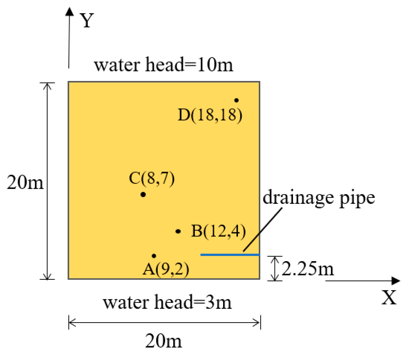
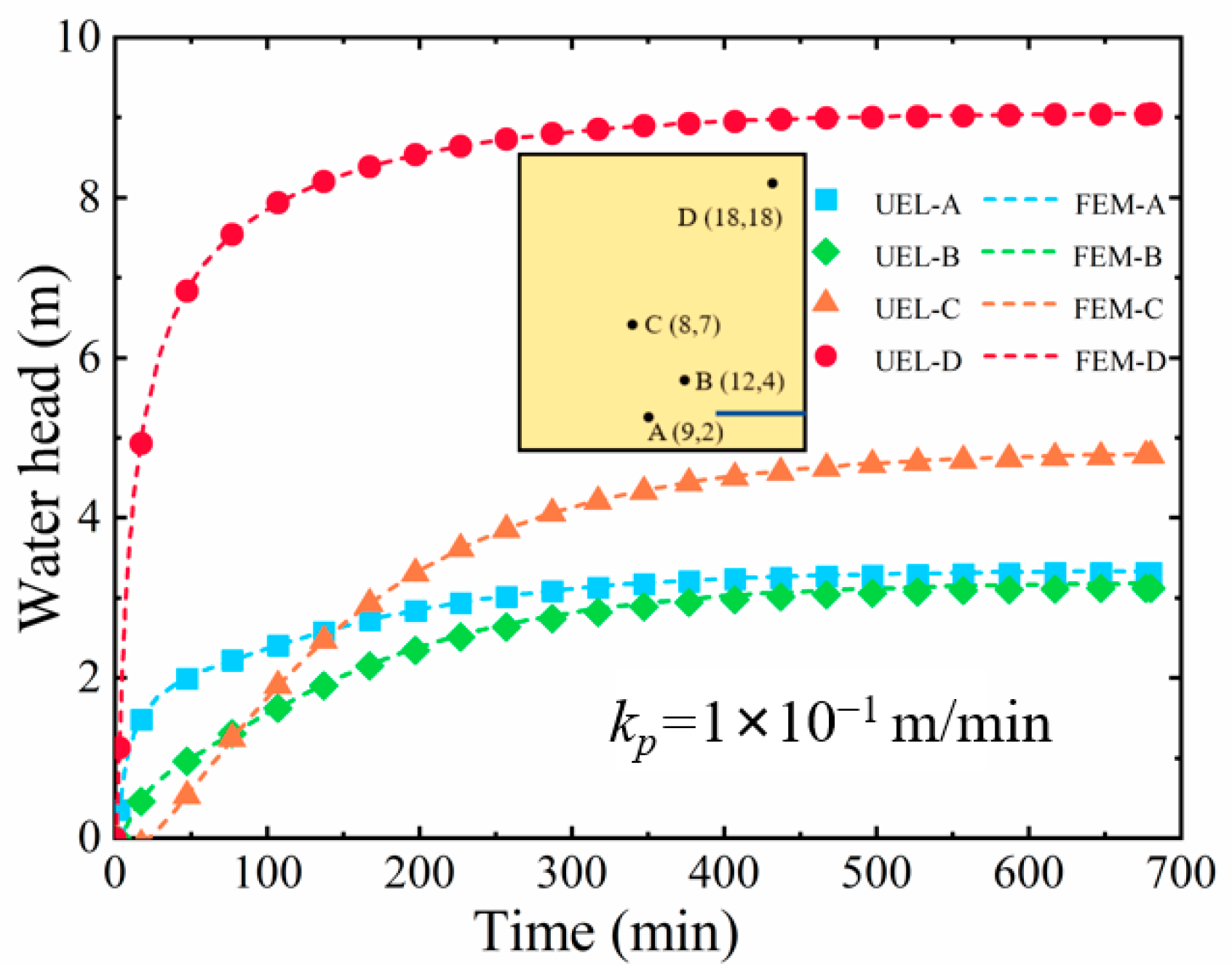
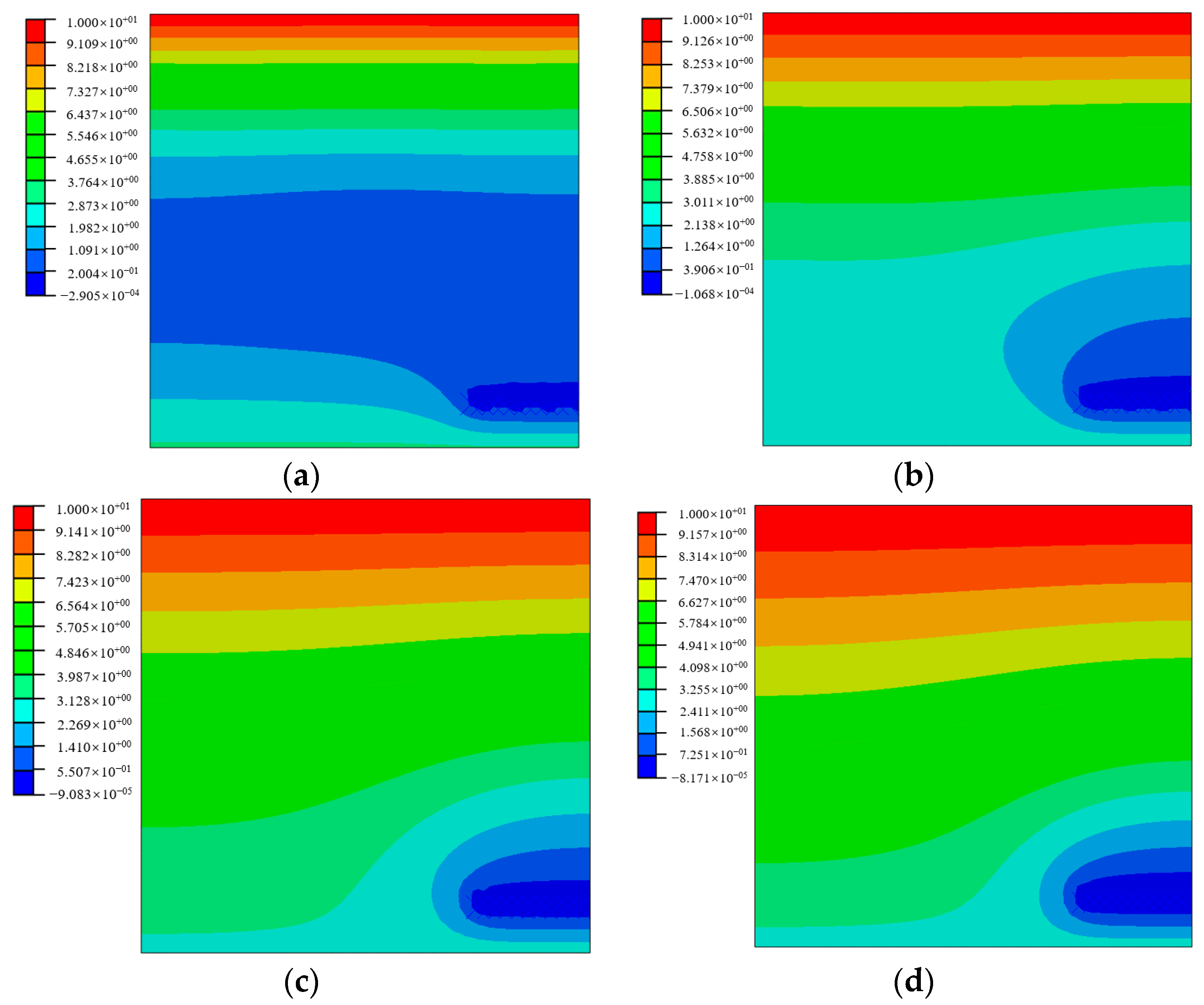
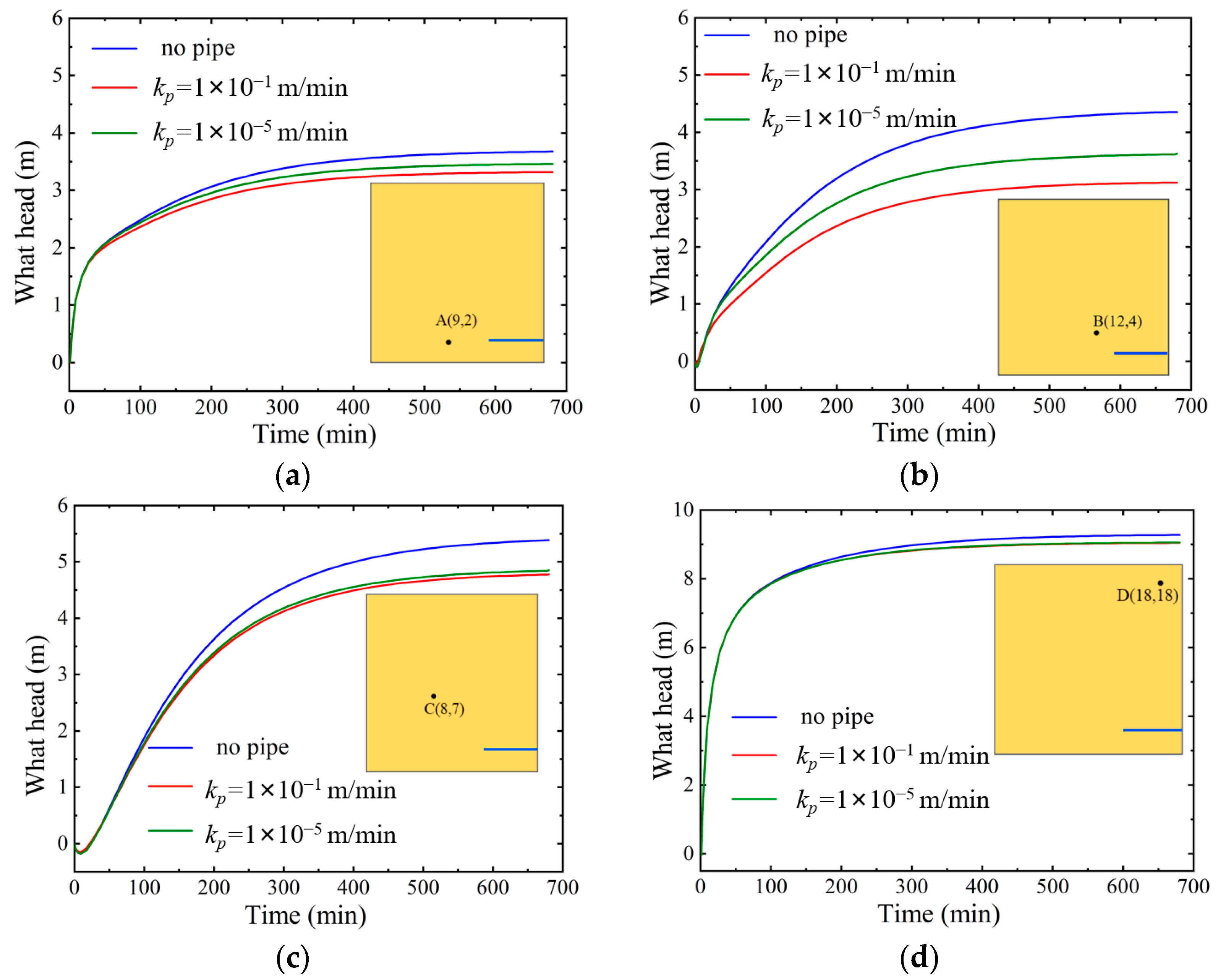
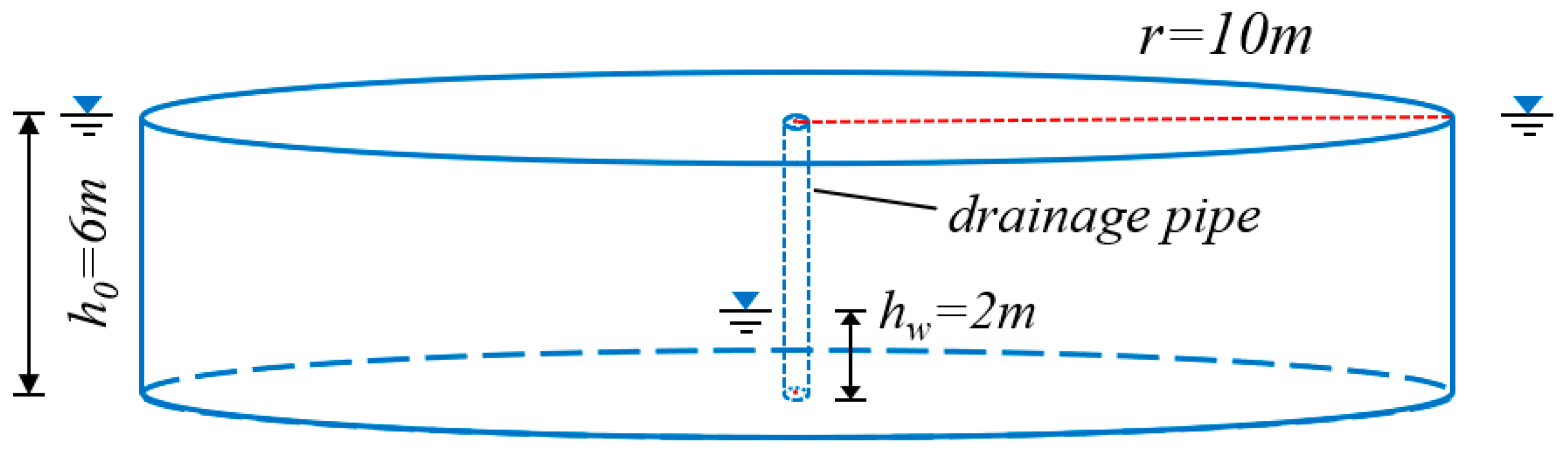
4.2. Transient State Seepage Simulation with a New Element Containing Drainage Pipe

To demonstrate the applicability of the seepage element containing drainage pipe proposed in this article in solving transient seepage problems, a square seepage area with a 5.0 m long drainage pipe horizontally buried at the bottom on the right side is employed, as shown in Figure 10. The water heads at the top and bottom boundaries of the seepage area are set to 10.0 m and 3.0 m, respectively; the permeability coefficients of the soil are taken as k = 3 × 10⁻⁴ m/min; the permeability coefficient, radius, and wall thickness of the wall of drainage pipe are taken as k_p = 1 × 10⁻¹ m/min, a = 0.1 m and t_wall = 0.01 m, respectively; and the storage coefficient is taken as s = 1 × 10⁻⁶ m⁻¹. Four monitoring points, A (9, 2), B (12, 4), C (8, 7), and D (18, 18), are selected for analysis. The total time for the seepage process was set to 680 min, using an automatic analysis step. The model established by the proposed seepage element containing drainage pipe is employed to simulate the seepage process. The water head evolution process at the monitoring points is tracked with a new element model, as shown in Figure 11. To compare and verify, a similar calculation is performed with the traditional element model. It can be seen that the water head at the monitoring points starts to increase rapidly, gradually slows down, and tends to stabilize over time. Moreover, points A and B closest to the drainage pipe are more affected by the drainage pipe, resulting in greater pressure release and smaller head values. The point C further away from the drainage pipe has a weaker impact, resulting in a higher water head. The point D farthest from the drainage pipe is least affected by the drainage pipe, resulting in the lowest water head loss. In addition, under the influence of gravity, the drainage pipe has a greater impact on the points above it than on the points on its left, especially in the initial stage. The almost identical results to the FEM model verify the effectiveness of the transient analysis of the proposed seepage element containing drainage pipe. To better observe the influence of drainage pipes on the pore pressure release, the water head distributions at four different moments, t = 50 min, 150 min, 300 min, and 680 min, are presented in Figure 12. It can be seen that the head distribution gradually stabilizes after 300 min, and the pressure in the area near the drainage pipe is released.

To further investigate the effect of the permeability of drainage pipes on the water head distribution, two drainage pipes with significant differences in permeability are selected, respectively given as k_p = 1 × 10⁻¹ m/min and k_p = 1 × 10⁻⁵ m/min. The evolution process of water heads at the four monitoring points is tracked with a new element model, as shown in Figure 13. It can be seen that the two monitoring points A and B closest to the drainage pipe are affected by the permeability of the drainage pipe, with point B having the greatest impact, while the monitoring points C and D far away from the drainage pipe are less affected by the permeability of the drainage pipe, and point D is almost unaffected.

Due to the small thickness of the pipe wall, the permeability of the drainage pipe is much higher than that of the soil matrix. In this case, even for two types of drainage pipes with significantly different permeabilities, the impact of the drainage pipe on the permeability pressure of the nearby area is not very significant.

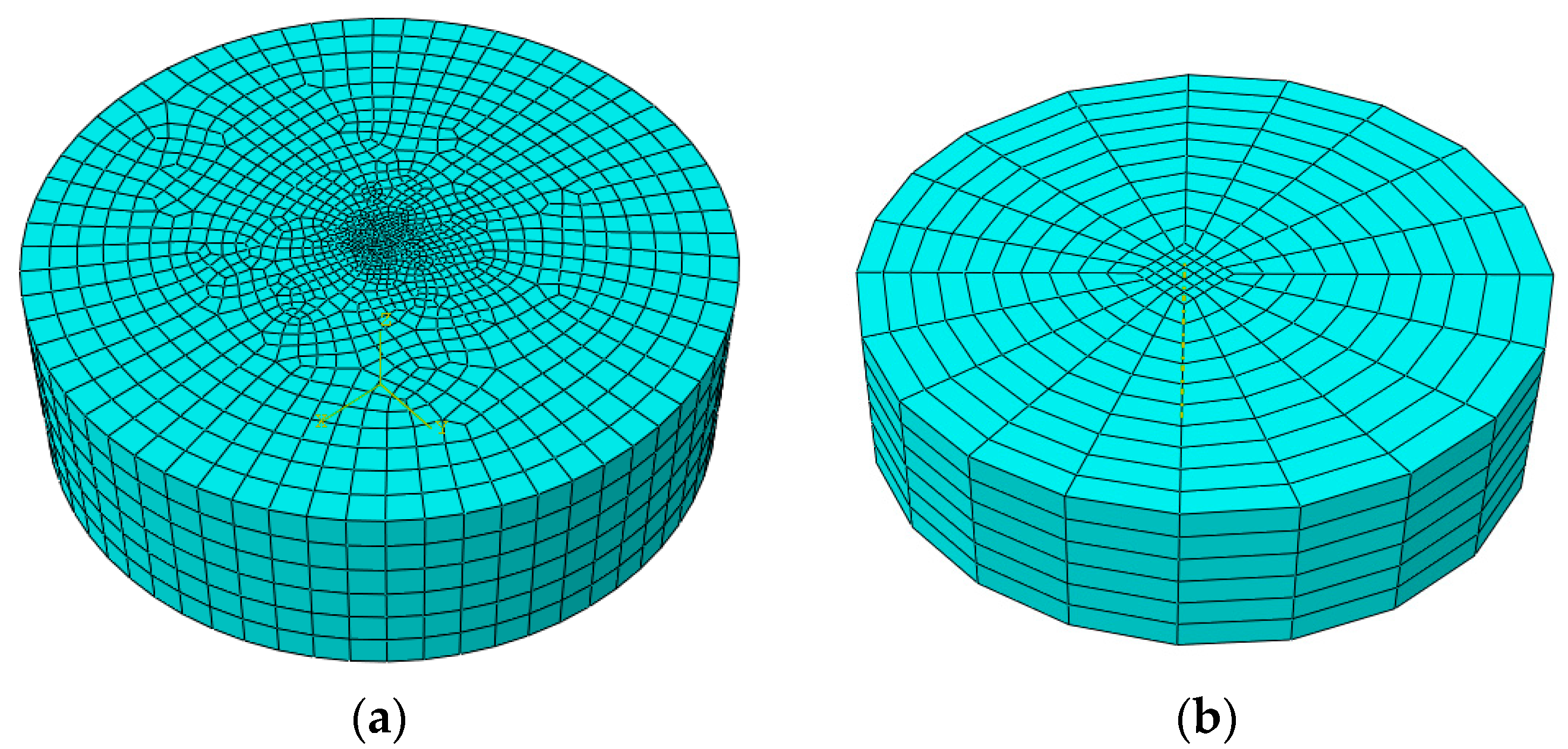
4.3. Comparison and Validation of the Element Containing Drainage Pipe in a Three-Dimensional Seepage Field

To validate the accuracy and effectiveness of the element containing drainage pipe in a three-dimensional seepage field, this section simulates a well flow model with a drainage pipe at the center. In this model, the aquifer thickness is 6 m, the drainage pipe radius is 0.05 m, the water level inside the pipe is 2 m, the radius of influence is 10 m, and the corresponding water level at the outer boundary is 6 m. Figure 14 shows the geometric shape of the model. Figure 15 shows the computational mesh of the model, where (a) has 7410 elements and 8883 nodes, and (b) has 1350 elements and 1729 nodes. It is evident that due to the very small radius of the drainage pipe, a relatively fine mesh is required when using traditional finite element modeling methods, which significantly increases the difficulty of mesh discretization. However, when using the UEL element developed in this paper to handle the model containing the drainage pipe, it is only necessary to replace the elements that the drainage pipe passes through with the elements containing the drainage pipe developed in this paper based on the model without the drainage pipe. This approach greatly reduces the number of elements and enhances computational efficiency.

Here, the UEL element developed in this paper is used to address the drainage pipe, and the calculated water head distribution is compared with the results obtained from the line-substitution hole method [18] (Bai et al., 2022). Figure 16 shows the water head distribution of the two methods in a top-down view. The water head contour lines are distributed in concentric circles, with streamlines flowing radially into the drainage pipe. It is also clear that, due to differences in mesh division, there are minor differences in water head values, but the overall computational results of the two methods are very close. This confirms that using the UEL element developed in this paper to handle the drainage pipe issue is appropriate.

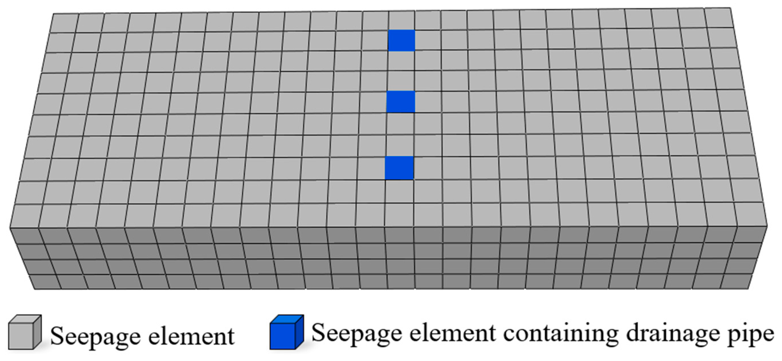
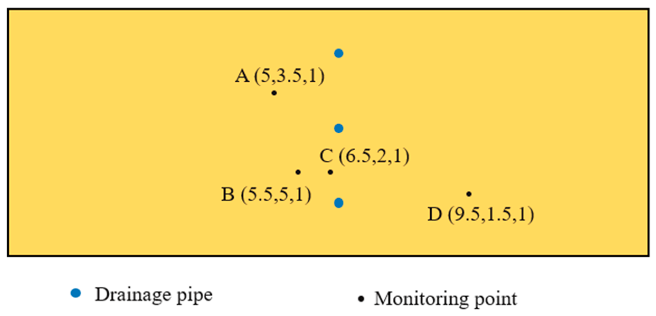
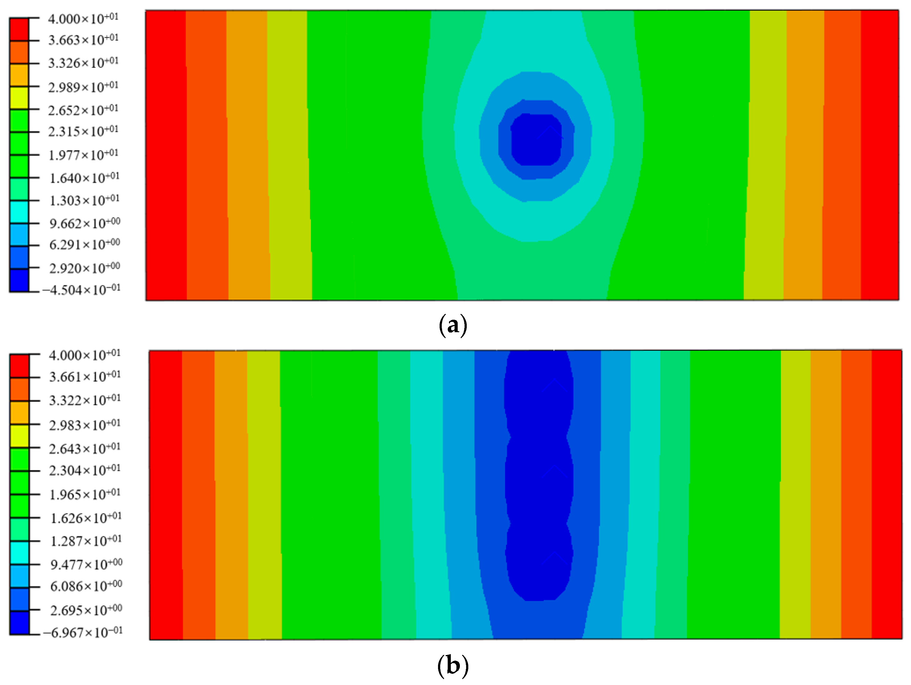
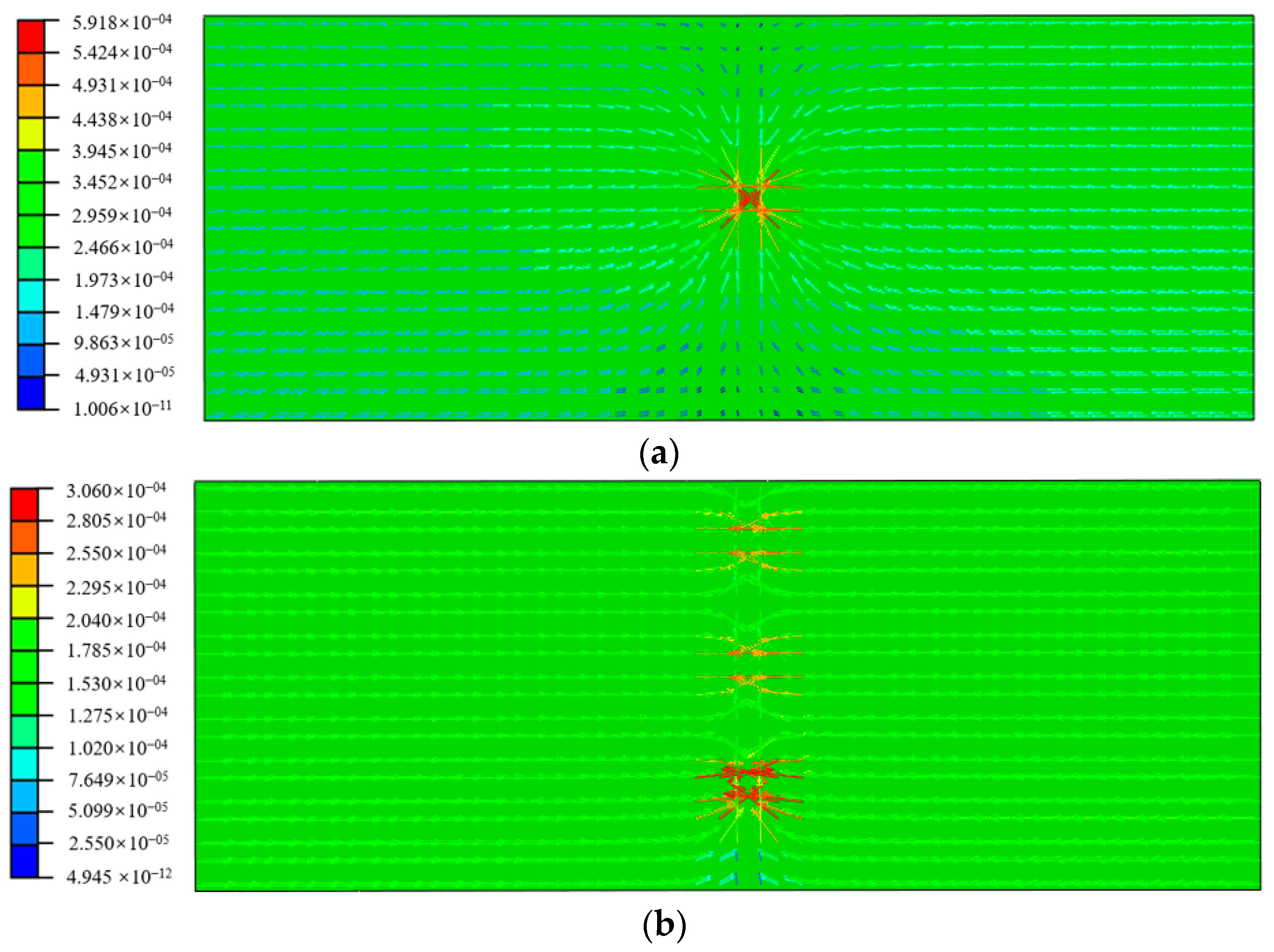
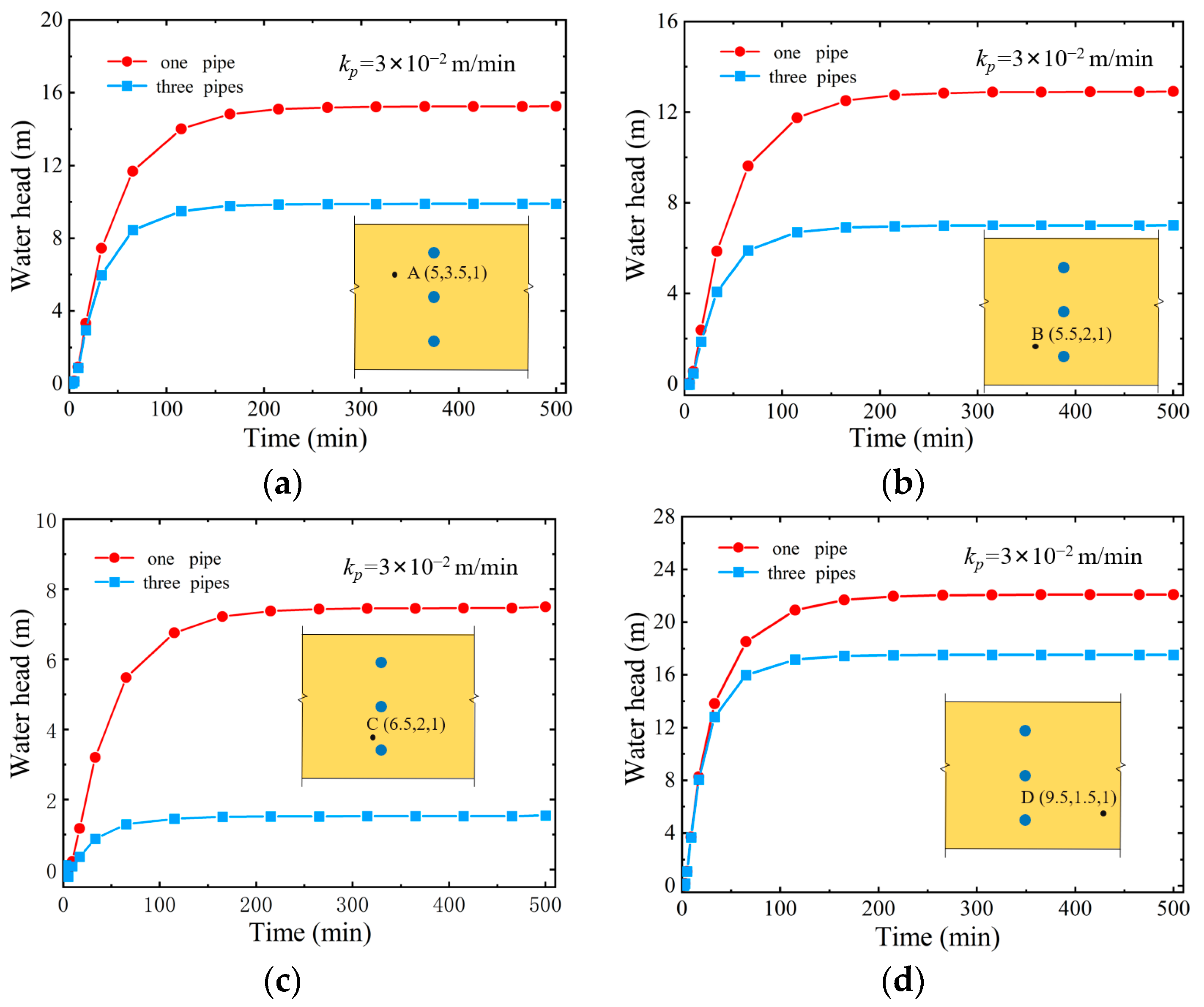
4.4. The Three-Dimensional Seepage Analysis of a Rock Mass Containing Drainage Pipes

A homogeneous rock mass with a length of 13.0 m, a width of 5.0 m, and a height of 2.0 m contains three pipes in central position, as shown in Figure 17, where the drainage pipes have a radius of 0.1 m and a thickness of 0.01 m and are buried at a depth of 1.5 m. The left and right sides of the rock mass are set at a fixed head boundary of h = 40.0 m; other surfaces are set as impermeable boundaries. The permeability coefficient of the rock mass and the drainage pipes is taken as k = 3.0 × 10⁻⁴ m/min and k = 3.0 × 10⁻² m/min, respectively. The finite element model of the rock mass is shown in Figure 18, where the seepage elements containing a drainage pipe are presented as small, blue blocks. Four monitoring points A, B, C, and D are all buried at a depth of 1.0m and arranged at different positions from the drainage pipes, as shown in Figure 19.

To investigate the drainage pressure relief effect of multiple drainage pipes, a simulation with a new element model is also conducted for a single drainage pipe. The stable water head distributions are presented in Figure 20, and the corresponding flow velocity distributions are shown in Figure 21.

From the comparison of Figure 20, it can be seen that the water head is greatly relieved near the drainage pipe, and the relief effect of the three drainage pipes is much larger than that of a single pipe, with a larger range of low water heads. From the flow velocity comparison in Figure 21, it can be found that the flow velocity near a single drainage pipe is higher than that of three drainage pipes, indicating that the aggregation effect of a single drainage pipe is more obvious under a fixed head boundary. However, in terms of the entire range, the high flow velocity distribution range for the case with three drainage pipes is wider, which indirectly indicates that the total water output of the drainage pipes affects the flow velocity distribution field.

For further comparison, the water head evolution at monitoring points for the case with a single water pipe and the case with three water pipes are tracked, respectively, as shown in Figure 22. From the comparison, it is not difficult to find that the water head of the monitoring points is much lower than that of a single drainage pipe in the case of three drainage pipes. Due to the superimposed effect of drainage pipes, the water head release at the monitoring point located in the middle of the two pipes is more significant. However, as the distance increases, this superimposed effect is not as obvious, as shown in Figure 22d.

It is obvious that the successful development of three-dimensional seepage element containing drainage pipe has greatly promoted the improvement of computational efficiency and provided an excellent simulation tool for the precise simulation of pore pressure relief facility systems in actual dam engineering.

5. Conclusions

In response to the problem of drainage pipes being too small in size compared to the solution domain, resulting in a huge mesh scale and low computational efficiency, this paper proposes a seepage element containing drainage pipe, where the permeability of the drainage pipe is taken as the third type of permeable conductivity condition and it is considered in the energy functional. The governing equations for steady-state and transient seepage element containing drainage pipes are derived using the variational principle, and the seepage matrix, equivalent nodal seepage array, and water storage matrix of the seepage element containing drainage pipe are obtained. By combining the user-defined element module UEL of Abaqus software, a secondary development is carried out on the proposed seepage element containing drainage pipe, leveraging the pre-processing and solving functions of Abaqus software, making the simulation of dyke dam engineering with drainage pipes more convenient. Three seepage examples are employed to verify the reliability and efficiency of the established seepage element containing drainage pipe. Simultaneously, the influence mechanism of the permeable conductivity capacity of the drainage pipe on the pore pressure reduction effect is also explored, including the superimposed effect of multi-drainage pipes. Some conclusions and further discussion are as follows.

(1)

In the proposed seepage element, the seepage matrix includes the drainage discharge contribution of the drainage pipe, and the element nodal seepage load array includes the permeable conductivity contribution of the drainage pipe. Therefore, in the newly proposed element model, it not only finely reflects the permeable conduction mechanism of the drainage pipe but also avoids the mesh meshing of the drainage pipe, ensuring calculation accuracy and improving calculation efficiency.

(2)

Taking the simulation of seepage in steady-state dyke dam, transient soil, and rock mass as examples, the reliability of the proposed element model and the correctness of the secondary development program UEL connecting to the Abaqus software are verified through comparative analysis with the calculation results of the traditional finite element model, providing convenience for the efficient use of the proposed seepage element containing drainage pipe.

(3)

By tracking the water head or pore pressure values of monitoring points near drainage pipes, it is found that the points closer to the drainage pipe are more affected by the drainage pipe, resulting in greater pressure release and smaller head values, while the points further away from the drainage pipe have a weaker impact, resulting in a higher water head. In addition, under the influence of gravity, the drainage pipe has a greater impact on the points above it.

(4)

The transient seepage of a three-dimensional rock mass with three drainage pipes under a fixed water head boundary is efficiently simulated using the proposed seepage element. By comparing the simulation results with those of a single drainage pipe, the combined pressure relief effect of multiple drainage pipes is explored. It is found that the pore pressure release at the position between the two pipes is more significant, and as the distance increases, this superimposed effect gradually weakens.

It should be pointed out that when dealing with drainage pipe issues using the element containing drainage pipe proposed in this paper, there are certain requirements for the regularity of the mesh. If the initial mesh distribution is too disordered or the drainage pipe is located on the boundary of the element, it is necessary to make improvements to the method presented in this paper. At the same time, the head interpolation function of the element does not reflect the sharp impact of the drainage pipe on the variation of the pressure head, so there is a slight error in the internal results of the element. However, the calculation results of the element nodes are still very accurate because the permeable transmission mechanism of the drainage pipes is considered accurately.

References

1. Cong, S.; Tang, L.; Ling, X.; Xing, W.; Geng, L.; Li, X.; Li, G.; Li, H. Three-Dimensional Numerical Investigation on the Seepage Field and Stability of Soil Slope Subjected to Snowmelt Infiltration. Water 2021, 13, 2729. [Google Scholar] [CrossRef]
2. Liu, W.; Luo, X.; Huang, F.; Fu, M. Uncertainty of the Soil–Water Characteristic Curve and Its Effects on Slope Seepage and Stability Analysis under Conditions of Rainfall Using the Markov Chain Monte Carlo Method. Water 2017, 9, 758. [Google Scholar] [CrossRef]
3. Chen, L.; Xi, B.; Dong, Y.; He, S.; Shi, Y.; Gao, Q.; Liu, K.; Zhao, N. Study on the Stability and Seepage Characteristics of Underwater Shield Tunnels under High Water Pressure Seepage. Sustainability 2023, 15, 15581. [Google Scholar] [CrossRef]
4. Zhang, C.; Chai, J.; Cao, J.; Xu, Z.; Qin, Y.; Lv, Z. Numerical Simulation of Seepage and Stability of Tailings Dams: A Case Study in Lixi, China. Water 2020, 12, 742. [Google Scholar] [CrossRef]
5. Yu, J.; Li, D.; Zheng, J.; Zhang, Z.; He, Z.; Fan, Y. Analytical Study on the Seepage Field of Different Drainage and Pressure Relief Options for Tunnels in High Water-Rich Areas. Tunn. Undergr. Space Technol. 2023, 134, 105018. [Google Scholar] [CrossRef]
6. Li, X.; Li, D. A Numerical Procedure for Unsaturated Seepage Analysis in Rock Mass Containing Fracture Networks and Drainage Holes. J. Hydrol. 2019, 574, 23–34. [Google Scholar] [CrossRef]
7. Aranda, J.Á.; Beneyto, C.; Sánchez-Juny, M.; Bladé, E. Efficient Design of Road Drainage Systems. Water 2021, 13, 1661. [Google Scholar] [CrossRef]
8. Sharma, V.; Fujisawa, K.; Murakami, A. Space-Time Finite Element Method for Transient and Unconfined Seepage Flow Analysis. Finite Elem. Anal. Des. 2021, 197, 103632. [Google Scholar] [CrossRef]
9. Sun, J.; Sun, H.; Lu, M.; Han, B. Finite-Difference Solution for Dissipation of Excess Pore Water Pressure within Liquefied Soil Stabilized by Stone Columns with Consideration of Coupled Radial-Vertical Seepage. Soil Dyn. Earthq. Eng. 2024, 176, 108328. [Google Scholar] [CrossRef]
10. Zhang, Y.T. Solving the seepage field with drainage holes using boundary elements. J. Hydraul. Eng. 1982, 7, 36–40. (In Chinese) [Google Scholar]
11. Fipps, G.; Skaggs, R.W.; Nieber, J.L. Drains as a Boundary Condition in Finite Elements. Water Resour. Res. 1986, 22, 1613–1621. [Google Scholar] [CrossRef]
12. Du, Y.L.; Xu, G.-A.; Huang, Y.H. The study of three-dimensional seepage analysis for the complex rock foundation. J. Hydraul. Eng. 1984, 8, 1–9. (In Chinese) [Google Scholar]
13. Wang, J.; Jiang, H.X. Simulating drainage holes with line sink drainage element. Chin. J. Geotech. Eng. 2008, 30, 677–684. (In Chinese) [Google Scholar]
14. Wang, L.; Liu, Z.; Zhang, Y.T. Analysis of seepage field near a drainage holes curtain. J. Hydraul. Eng. 1992, 12, 15–20. (In Chinese) [Google Scholar]
15. Chen, Y.F.; Zhou, C.B.; Zheng, H. A numerical solution to seepage problems with complex drainage systems. Comput. Geotech. 2008, 35, 383–393. [Google Scholar] [CrossRef]
16. Xu, Z.G.; Cao, C.; Li, K.H.; Chai, J.R.; Xiong, W.; Zhao, J.Y.; Qin, R.G. Simulation of drainage hole arrays and seepage control analysis of the Qingyuan Pumped Storage Power Station in China: A case study. Bull. Eng. Geol. Environ. 2019, 78, 6335–6346. [Google Scholar] [CrossRef]
17. Su, H.Z.; Li, J.Y.; Wen, Z.P.; Guo, Z.Y.; Zhou, R.L. Integrated certainty and uncertainty evaluation approach for seepage control effectiveness of a gravity dam. Appl. Math. Model. 2019, 65, 1–22. [Google Scholar] [CrossRef]
18. Bai, C.S.; Chai, J.R.; Xu, Z.G.; Qin, Y. Numerical simulation of drainage holes and performance evaluation of the seepage control of gravity dam: A case study of Heihe reservoir in China. Arab. J. Sci. Eng. 2022, 47, 4801–4819. [Google Scholar] [CrossRef]
19. Zhu, B.F.; Li, Y.; Xu, P. Substitution of the curtain of drainage holes by a seeping layer in the three dimensional finite element analysis of seepage field. Water Resour. Hydropower Eng. 2007, 38, 24–28. (In Chinese) [Google Scholar]
20. Hu, J.; Chen, S.H. Air element method for modeling the drainage hole in seepage analysis. Rock Soil Mech. 2003, 24, 281–287. (In Chinese) [Google Scholar]
21. Chen, S.H.; Shahrour, I. Composite Element Method for the Bolted Discontinuous Rock Masses and Its Application. Int. J. Rock Mech. Min. Sci. 2008, 45, 384–396. [Google Scholar] [CrossRef]
22. Chen, S.H.; Feng, X.M.; Isam, S. Numerical Estimation of REV and Permeability Tensor for Fractured Rock Masses by Composite Element Method. Num. Anal. Methods Geomech. 2008, 32, 1459–1477. [Google Scholar] [CrossRef]
23. Chen, S.H.; Qiang, S.; Shahrour, I.; Egger, P. Composite Element Analysis of Gravity Dam on a Complicated Rock Foundation. Int. J. Geomech. 2008, 8, 275–284. [Google Scholar] [CrossRef]
24. Chen, S.H.; Xue, L.L.; Xu, G.S.; Shahrour, I. Composite element method for the seepage analysis of rock masses containing fractures and drainage holes. Int. J. Rock Mech. Min. Sci. 2010, 47, 762–770. [Google Scholar] [CrossRef]
25. Chen, S.H.; Feng, X.M. Composite element model for rock mass seepage flow. J. Hydrodynam. (Ser. B) 2006, 18, 219–224. [Google Scholar]
26. Vincent, K.K.; Muthama, M.N.; Muoki, S.N. Darcy’s law equation with application to underground seepage in earth dams in calculation of the amount of seepage. Am. J. Appl. Math. Stat. 2014, 2, 143–149. [Google Scholar] [CrossRef]
27. Lai, Y.M.; Wu, Z.; Zhu, Y.; Zhu, L. Nonlinear analysis for the coupled problem of temperature and seepage fields in cold regions tunnels. Cold Reg. Sci. Technol. 1999, 29, 89–96. [Google Scholar] [CrossRef]
28. Zhou, Z.; Ling, T.; Huang, F.; Zhang, M. The Face Stability Analysis of Shield Tunnels Subjected to Seepage Based on the Variational Principle. Sustainability 2022, 14, 16538. [Google Scholar] [CrossRef]
29. Wise, J.; Hunt, S.; Al Dushaishi, M. Prediction of Earth Dam Seepage Using a Transient Thermal Finite Element Model. Water 2023, 15, 1423. [Google Scholar] [CrossRef]
30. Fukuchi, T. Numerical Analyses of Steady-State Seepage Problems Using the Interpolation Finite Difference Method. Soils Found. 2016, 56, 608–626. [Google Scholar] [CrossRef]
31. Lipnikov, K.; Manzini, G.; Svyatskiy, D. Analysis of the Monotonicity Conditions in the Mimetic Finite Difference Method for Elliptic Problems. J. Comput. Phys. 2011, 230, 2620–2642. [Google Scholar] [CrossRef]
32. Xing, Y.; Yao, L.; Ji, Y. A Solution Strategy Combining the Mode Superposition Method and Time Integration Methods for Linear Dynamic Systems. Acta Mech. Sin. 2022, 38, 521433. [Google Scholar] [CrossRef]
33. Yang, Y.; Zhang, Z.; Feng, Y.; Wang, K. A Novel Solution for Seepage Problems Implemented in the Abaqus UEL Based on the Polygonal Scaled Boundary Finite Element Method. Geofluids 2022, 2022, 5797014. [Google Scholar] [CrossRef]
34. Kshirsagar, S.; Nguyen-Xuan, H.; Liu, G.R.; Natarajan, S. An SFEM Abaqus UEL for Nonlinear Analysis of Solids. Int. J. Comput. Methods 2023, 20, 2350003. [Google Scholar] [CrossRef]
Figure 1. Drainage pipe in soil elements. (a) Two-dimensional element; (b) Three-dimensional element.
Water 16 01440 g001
Figure 2. Drainage pipe structure.
Water 16 01440 g002
Figure 3. The framework of user subroutines UEL.
Water 16 01440 g003
Figure 4. Flow chart of the UEL subroutine for the element containing drainage pipe.
Water 16 01440 g004
Figure 5. The declaration and definition of the user element.
Water 16 01440 g005
Figure 6. The dimensions of a dyke dam, the buried drainage pipe, and the monitoring points.
Water 16 01440 g006
Figure 7. The results for no drainage pipe. (a) Pore pressure distribution (kPa); (b) The corresponding infiltration surface.
Water 16 01440 g007
Figure 8. The results simulated by the traditional finite element model for kp = 1 × 10⁻⁴ m/s. (a) Pore pressure distribution (kPa); (b) The corresponding infiltration surface.
Water 16 01440 g008
Figure 9. The results simulated by a new element model for kp = 1 × 10⁻⁴ m/s. (a) Pore pressure distribution (kPa); (b) The corresponding infiltration surface.
Water 16 01440 g009
Figure 10. Transient state seepage model with drainage pipe.
Water 16 01440 g010
Figure 11. The water head evolution process at the monitoring points tracked by the new element model (UEL within Abaqus) and FEM.
Water 16 01440 g011
Figure 12. Water head distribution at different moments with the new element model. (a) 50 min; (b) 150 min; (c) 300 min; (d) 680 min.
Water 16 01440 g012
Figure 13. The water head evolution at monitoring points for different permeabilities of drainage pipes. (a) The water head evolution at monitoring point A; (b) The water head evolution at monitoring point B; (c) The water head evolution at monitoring point C; (d) The water head evolution at monitoring point D.
Water 16 01440 g013
Figure 14. Well flow model.
Water 16 01440 g014
Figure 15. Calculation mesh. (a) Traditional FEM; (b) Containing the UEL element.
Water 16 01440 g015
Figure 16. Top view of the water head distribution of the well flow model (m). (a) Results by the line-substitution hole method [18] (Bai et al., 2022); (b) Results by the element containing drainage pipe.
Water 16 01440 g016
Figure 17. The dimensions of the rock mass and the buried drainage pipe.
Water 16 01440 g017
Figure 18. The finite element mesh for the rock mass.
Water 16 01440 g018
Figure 19. The monitoring points.
Water 16 01440 g019
Figure 20. The water head distribution (m) (a) with a single drainage pipe and (b) with three drainage pipes.
Water 16 01440 g020
Figure 21. The seepage flow velocity distribution (m/min) (a) with a single drainage pipe and (b) with three drainage pipes.
Water 16 01440 g021
Figure 22. The water head evolution at monitoring points with single and three drainage pipes. (a) The water head evolution at monitoring point A; (b) The water head evolution at monitoring point B; (c) The water head evolution at monitoring point C; (d) The water head evolution at monitoring point D.
Water 16 01440 g022