Article

Water Resource Utilization Assessment in China Based on the Dynamic Relationship between Economic Growth and Water Use

1
Faculty of Geographical Science, Beijing Normal University, Beijing 100875, China
2
School of Resource & Environment, Hunan University of Technology and Business, Changsha 410205, China
3
Nanjing Institute of Environmental Sciences, Ministry of Ecology and Environment of the People’s Republic of China, Nanjing 210042, China
4
Changsha Social Laboratory of Artificial Intelligence, School of Science, Hunan University of Technology and Business, Changsha 410205, China
*
Authors to whom correspondence should be addressed.
Water 2024, 16(10), 1325; https://doi.org/10.3390/w16101325
Submission received: 20 March 2024 / Revised: 19 April 2024 / Accepted: 26 April 2024 / Published: 7 May 2024
(This article belongs to the Special Issue Water Governance and Sustainable Water Resources Management)

Abstract

:
Water scarcity has significantly hampered China’s economic, social, and environmental development. Ensuring sustainable water utilization is crucial given the mounting water stress accompanying continuous economic growth. A quantitative water resource forewarning model was constructed using the vector autoregressive (VAR) model. By analyzing the key indicators related to water systems and GDP data from 2001 to 2022, the VAR model revealed the long-term dynamic correlation between water consumption and economic growth using generalized impulse response, co-integration, and predictive variance decomposition analyses. The results revealed the presence of a long-term equilibrium between water consumption and economic growth, with a stable co-integration relationship and an optimal lag period of one year. The positive impact of water consumption on economic development increased during the 2001–2022 period, indicating a rising dependence of GDP on water resources. Water usage rose with economic development, while the water resource carrying capacity remained high and continued to grow. Based on the generalized impulse response, co-integration, and predictive variance decomposition analyses, this study predicted water-use-related indicators, providing vital early warnings for China’s water environment carrying capacity from 2023 to 2050. This enabled informed decision-making and fostered sustainable water management practices for the future.

1. Introduction

With swift population increase and economic growth, the increasing water demand placed immense pressure on the water system [1,2]. Over the last several decades, China’s Gross Domestic Product (GDP) has experienced significant growth, with a staggering increase of more than 330% at constant prices from 1978 (CNY 365 billion) to 2022 (CNY 1210.20 billion) [3]. This tremendous growth has led to resource security challenges, positioning China as one of the largest economies and resource consumers in the world [4]. However, this growth also exacerbates the issue of water scarcity, with total water use surging from 103 trillion liters in 1950 to 599.82 trillion liters in 2022. Meanwhile, the total available water resources remain relatively stable and unevenly distributed, with the south accounting for more than 80% of the total, while the north only accounted for around 20%. Therefore, China is classified as a ’water-scarce’ country according to the United Nations Environment Programme [5].
Statistics reveal that China’s per capita water consumption is expected to reach only 425 m3 in 2022, less than half of the global average [6]. Moreover, an estimated 440 out of 669 Chinese cities experience water shortages, with 110 of them facing ‘serious’ scarcity [7]. Additionally, a nationwide survey of 1935 sampling sites at China’s rivers, lakes, and reservoirs in 2018 revealed that 29% of them had poor water quality [8]. And around 300 million rural inhabitants lack access to safe drinking water [9]. These water shortages and related environmental issues are becoming a significant impediment to China’s economic sustainable development [7,10].
Understanding the relationship between water resources and economic growth is crucial for exploring pathways to achieve sustainable water utilization and sustainable economic development [11,12,13]. Sustainable water utilization represents water consumption practices that do not deplete water stocks and impair water ecosystems [14]. It has been discovered that the interaction between water resources and economic growth is bidirectional: On one hand, economic growth is paired with a rise in water consumption. However, when economic growth surpasses a certain critical value, and with advancements in technology, the optimization of industrial structure, and changes in economic growth patterns, the speed of increase in water usage starts to decline [15,16]. On the other hand, water usage also affects economic growth, as the limited nature of water resources inevitably impacts investment and the economic growth speed in subsequent stages [17,18]. Many scholars have concurred that economic growth led to a rise in total water use [19,20,21]. Similarly, studies have indicated that water resources played a crucial role in driving economic growth. For instance, Alrwis et al. [22] assessed the effect of water scarcity on Saudi Arabia’s national economic growth and concluded that water scarcity affected GDP by reducing crop areas and agricultural output.
Furthermore, researchers have explored the implications of economic growth on water resources. Zhao et al. [23] found a significant inverted U-shaped relationship between water consumption and economic growth across different regions in China for the period 2003 to 2014. Zhang et al. [24] demonstrated a curved, inverted U-shaped correlation between per capita industrial water usage and GDP across different regions in China using the triple reduction model. Using a simultaneous equation model, Hao et al. [25] analyzed the correlation between water consumption and economic growth in 29 Chinese provinces from 1999 to 2014 and discovered an N-shaped relationship between per capita water use and per capita GDP in China.
The vector autoregression (VAR) model, introduced by Sims [26], provides a new macro-econometric framework to capture complex dynamic interrelationships among macroeconomic variables over flexible time series. Traditional univariate autoregression is characterized by a linear model with single equation and single variable, whereas the VAR model is a linear model with multiple equations and variables. In the VAR model, each variable is explained both by its lagged values and by the current and past values of the other variables. This provides a methodical approach of capturing the diverse dynamics across multiple time series. VAR models allow for the analysis of interactions between several variables through impulse response. Scholars have utilized the VAR model in various studies related to renewable energy consumption, greenhouse gases emission, economic growth, and other factors influencing economies and environmental outcomes [27,28,29].
The prediction and warning of the overloading status of the water environment carrying capacity involves assessing the deviation of water quality and quantity from the ideal state. It comprises three main components: water use assessment, water use change prediction, and regulation. An effective approach to water use assessment is the comprehensive warning index system [5,30]. When constructing the early warning indicator system, it is beneficial to refer to the evaluation index system for the water environment carrying capacity [31]. This system incorporates the general principles of water environment assessment while considering the complex characteristics of regional water resources systems. A comprehensive regional early warning indicator system for sustainable water resource utilization encompasses not only indicators related to the water resources system but also social, economic, and ecological indicators.
In this paper, we employed water and economic data from the 2001–2022 period and utilized the VAR model to explore the dynamic correlation of economic growth and water consumption. Based on the relationship results, we have predicted China’s water use changes during 2023–2050. Additionally, we proposed an early warning system to assess water utilization sustainability for analyzing the overloading status of water resources carrying capacity during 2023–2050. By analyzing the internal dependence and causal relationship between water consumption and economic growth, the paper aims to offer guidance for assessing the sustainability of water resources and early warning for potential water overload in the future, serving as a foundation for policymaking to ensure water sustainability.

2. Methodology

2.1. VAR Model

2.1.1. The Establishment of the VAR Model

By formulating a model where each endogenous variable (a variable explained by the equations) is considered as a function of the lagged values of all endogenous variables, the VAR method avoids the necessity for a structured model. The following equation shows the VAR(p) model:
f t = α 1 f t 1 + α 2 f t 2 + + α p f t p + β g t + ε t
where the f t is an n × 1 vector of the endogenous variables; f t 1 , f t 2 , f t p are the lag periods of the f t ; α 1 , α 2 , α p represent the matrices of suitable dimensions containing the model’s unknown parameters of the f t ; g t is the exogenous variable (a variable not explained within the model); β refers to the expected coefficient of the g t ; and ε t is an n × 1 vector of exogenous shocks.
The VAR model can be transformed into a matrix:
f 1 t f 2 t f k t = α 1 f 1 t 1 f 2 t 1 f k t 1 + α 2 f 1 t 2 f 2 t 2 f k t 2 + + α p f 1 t p f 2 t p f k t p + β g 1 t g 2 t g k t + ε 1 t ε 2 t ε k t
where f 1 t , f 2 t , , f k t are endogenous variables, and they are associated with the same period. They are calculated by their lagged variables, exogenous variables, and exogenous shocks. We convert the equation into a matrix for the convenience of observing the calculation results of each variable.

2.1.2. Time Difference Correlation Analysis (TDCA)

The TDCA method utilizes the time difference correlation coefficient (TDCC) to determine the average relationship between two or more sequences in the entire time series. The TDCC ranges from −1 to 1, where 0 indicates no correlation, −1 indicates complete negative correlation, and 1 indicates complete positive correlation. The correlation coefficient reflects the degree of linear relationship between economic growth and water use. By quantifying the temporal relationship, it is judged whether a sequence is preceded or delayed relative to another sequence [32].
The process is as follows: Firstly, a warning indicator that comprehensively reflects the current sustainable utilization of water resources is used as a benchmark indicator J, and the benchmark indicator is fixed, and other selected indicators I are moved forward or backward in time relative to the benchmark indicator for several years. Then, the TDCC between the benchmark and the moved sequence is calculated. The maximum number of years of movement corresponding to the resulting maximum correlation coefficient is considered as the lead or delay of the indicator. At the same time, based on this, the index of the selected indicators is divided into the leading and lag periods. The TDCA method has characteristics such as quantitative calculation, high precision, and low sequence length requirement.
The specific calculation method is as follows:
Assume that the benchmark is J = j 1 , j 2 , . . . , j n , the selected indicator is I = i 1 , i 2 , . . . , i n , the TDCC is Rl:
R l = l = 1 k t i t + l i ¯ j t j ¯ l = 1 k t i t + l i ¯ 2 l = 1 k t j t j ¯ 2
l = 1 t 0 1 t t < 0 , t = 0 , ± 1 , ± 2 , , ± M B
Here, t = 0 means the indicators are synchronized. When taking a negative value, it means moving forward or pre-emption; when it is positive, it means hysteresis, which is called lag number or time difference number. i ¯ and j ¯ refer to the mean value of indicator I and J. MB refers to the years of movement. kt represents the data volume after the I and J indicators are aligned. In the calculation of the index, the TDCC under various delay numbers is computed. Among these Rl values, the maximum value R′l after taking the absolute value is selected, and the corresponding delay number ′l signifies either the leading or lagging period. During the inspection process, the closer R′l is to 1, the more ideal it is, and the fluctuation of I and J is closer. If Rl is the largest at t = 0 , the index I is the synchronization index of the reference index J; if it is the largest when t < 0 , then I is the hysteresis index of the reference index J.

2.2. Water Sustainable Utilization Assessment Index System

2.2.1. Indicator Selection

In this study, a representative index variable was selected for economic growth and water resource utilization for quantitative analysis. GDP represents the production results of all resident economic units in a country or region and covers all industries of the national economy. It is a measure of the total economic activity between countries and regions [33]. Therefore, in this study, GDP is utilized as an economic growth indicator, measured in units of CNY 100 million.
Based on the water usage structure, water resources are categorized into four types: domestic water, agricultural water, industrial water, and ecological water. Considering the ecological water consumption is small and ecological water use has been used as a separate indicator for statistics in recent years, for the convenience of research, this paper classifies it into domestic water. Therefore, this paper selects total water consumption (TWC), domestic water usage, industrial water usage, and agricultural water usage as water use indicators (unit: 100 million m3).
In addition, indicators such as the ratio of sewage treatment facilities (STFs) per capita of GDP, the amount of STFs, and the total amount of water resources were chosen to evaluate both water resources carrying capacity and water environmental carrying capacity.

2.2.2. Early Warning Indicators for Sustainable Use of Water Resources

In the early warning indicator system, the indicator’s impact on the sustainability of regional water consumption is not consistent over time. Some indicators have an impact on current water use, while others take some time to have an impact on it. Based on many studies, this paper uses water resources status, economic, and social indicators to reflect the characteristics, development, and consumption of regional water resources, and ultimately the status of regional water sustainability is measured.
Therefore, based on the selected 26 indicators (Table 1), it is necessary to further distinguish the order in which these indicators influence the sustainable utilization of water resources. These indicators were categorized into three types: leading, synchronous, and lagging indicators. This paper screened the early warning indicators for the sustainable utilization of water resources based on their categorization [34,35,36].
The early warning indicator system hierarchy structure consists of three levels (see Figure 1): target layer (A), criterion layer (S), and indicator layer (R).

2.2.3. Early Warning Indicator Hierarchy Model

In this paper, Eviews 5.1 was utilized for calculating the TDCC between the police index and the above-mentioned 26 warning indicators. Then, according to the calculated TDCC, the selection of index was determined, and the finally selected indicators were classified. The effective TDCC of each index should generally be greater than 0.5, and the time difference between the leading and lag indicators is usually more than three years.
Classification of indicators: If the maximum correlation coefficient corresponding to the indicator is obtained in the lead period of the indicator, then the indicator is classified as the leading indicator. On the other hand, if the maximum correlation coefficient corresponding to the indicator is obtained in the delay period of the indicator, then the indicator is classified as the lagging indicator. From the results, the nature category of each indicator was determined by examining both the indicator itself and the absolute value of the TDCC of the water resource availability index.
Based on the above results, 16 indicators were classified as the leading indicators, and there were 3 synchronous indicators (population, per capita GDP, and total water resources), while the remaining 13 were lagging indicators.

2.3. Data Sources

The indicators mentioned above were obtained directly or indirectly from sources such as the China Water Resources Bulletin [37] and the China Statistical Yearbook (CSY) [3]. And the data include major provinces and cities in China. However, it is worth noting that the population data obtained from the CSY, including data from the past six Chinese population censuses, showed limited comparability across various periods and regions [38]. To address this issue, some scholars adjusted both the urban and the total population data for the period 2001 to 2022 in China [39]. Regarding the economic data, we calculated the growth rates in comparison to the previous year and then adjusted the China’s GDP figures from 2001 to 2022 into constant prices in 1997.

3. Results and Discussion

3.1. VAR Model Establishment and Basic Test

3.1.1. Unit Root Test

Aiming at avoiding spurious regression and ensuring the stability of all sequences [40,41], we conducted an Augmented Dickey–Fuller (ADF) test for GDP (LOGJ) and TWC (LOGI). The findings (Table 2) indicated that both variables were second-order single-stationary sequences (DDLOGI and DDLOGJ).

3.1.2. Cointegration Test

Given that the original variables were in an unstable state, it was essential to conduct further cointegration tests to ascertain whether a long-term equilibrium relationship existed among these variables. The cointegration test results (see Table 3) revealed the existence of a cointegration relationship among these variables.

3.1.3. Choice of Lag Period

Choosing the lag period was essential for establishing the VAR model. We adjusted the total water consumption (TWC) and lag period of GDP using six inspection criteria (LogL, HQ, SC, FPE, LR, AIC). Following the rule of choosing the minimum values of HQ, SC, FPE, and AIC, we determined that the optimal lag order for GDP and TWC was 1 (Table 4).

3.1.4. The Parameters Result in VAR

Based on the results of unit root test and lag period selection mentioned above, the VAR model was formulated as (5), which represented the relationship between GDP and TWC. The stationary sequences obtained from the tests were used as inputs to the model, and the model’s parameters were estimated using the least squares method.
D L O G J 1 = 0.2153 C + 0.0452 L O G I 1 t 1 + 0.9618 L O G J 1 t 1
Table 5 illustrated that the test results for the VAR model were highly significant. The AIC and SC values were very low, and the fitting effect was better.

3.1.5. The Test of Model Stability

After conducting the tests, it was found that all root moduli were below 1, indicating that the established VAR model of GDP and TWC was stable. As a result, various tests based on the VAR model proved to be effective (Table 6 and Figure 2).

3.1.6. Granger Causality Test (GCT)

The GCT was employed to determine the chronological order between economic variables. However, it does not necessarily indicate a causal relationship, which necessitates comprehensive judgment based on theory, experience, and the model. We conducted the Granger Causality Test between GDP and total water consumption (Table 7). By combining the principle of the Granger Causal Analysis, a one-way causal relationship between GDP and TWC was clearly established.

3.2. Pulse Effect Analysis

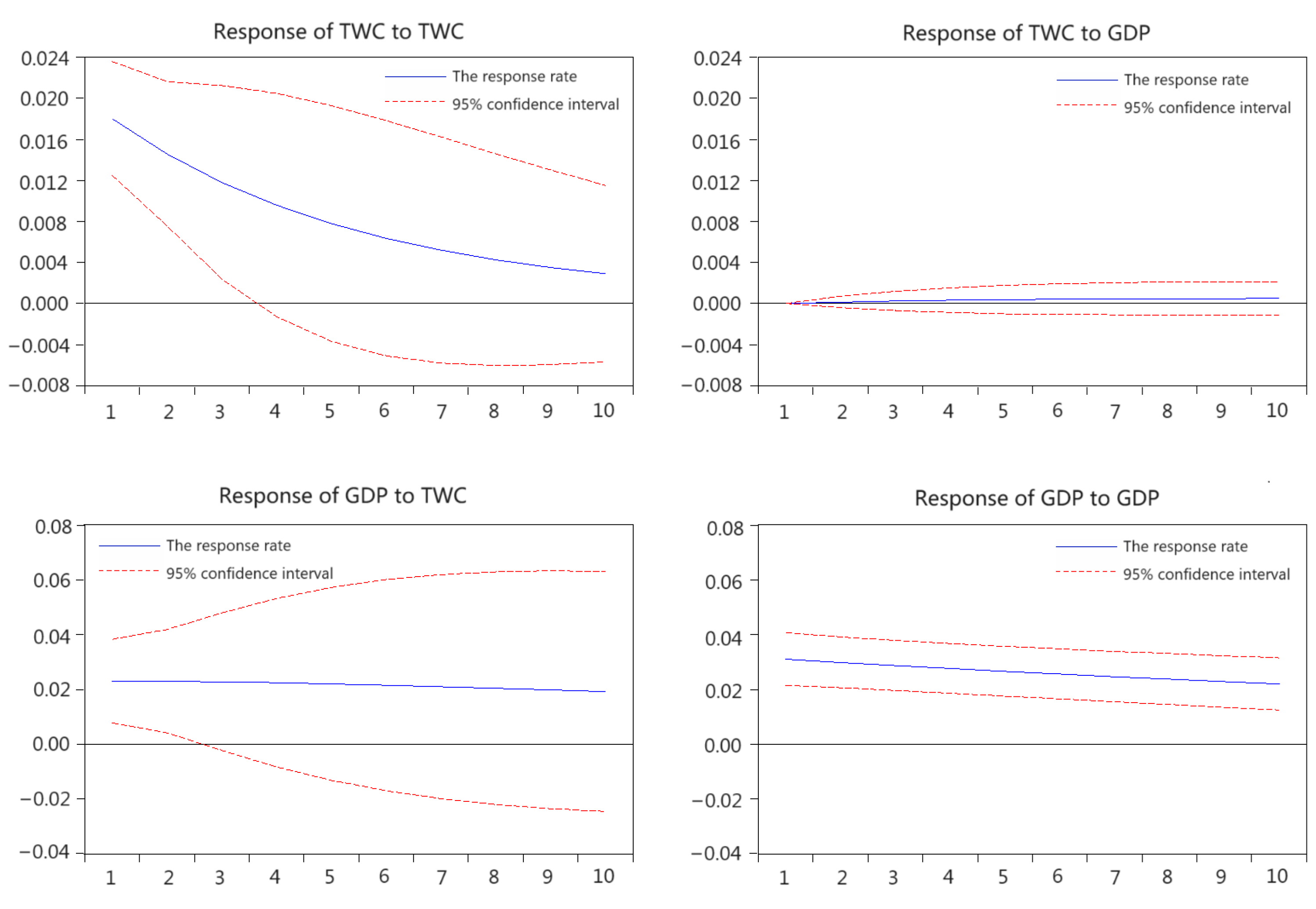
Figure 3 illustrated the mutual influence and interactions between GDP and TWC. Regarding how GDP responded to TWC, the DDLOGI value was 0 during the initial period. However, it exhibited positive values that gradually decreased in magnitude in the subsequent second, third, fourth, and fifth periods. This indicated that a decreasing dependence of GDP on TWC over time.
Conversely, when concerning how TWC responded to GDP, DDLOGJ was 0 in the first period. It turned positive in the second period and remained positive in the third period. Subsequently, the response showed increasing convergence, implying that the continued economic growth had a diminishing impact on the further development of water resources.

3.3. Analysis of Variance Decomposition

3.3.1. Analysis of Variance Decomposition of GDP and TWC

In Figure 4, the variance decomposition of GDP and TWC was presented. It was observed that TWC contributed less to the variance of GDP, which was consistently maintained below 5%. The variation in GDP was mainly influenced by its own dynamics.
On the other hand, the contribution of GDP to TWC was notably high. Except for the first two periods, where it was less than 30%, the contribution increased over time and gradually exceeded 30%. After the fifth period, it experienced a slight increment and then stabilized. Ultimately, it approached and reached close to 40%, indicating that the growth of the economy had a significant impact on water consumption.

3.3.2. Forecast the TWC and GDP Changes of 2023–2050

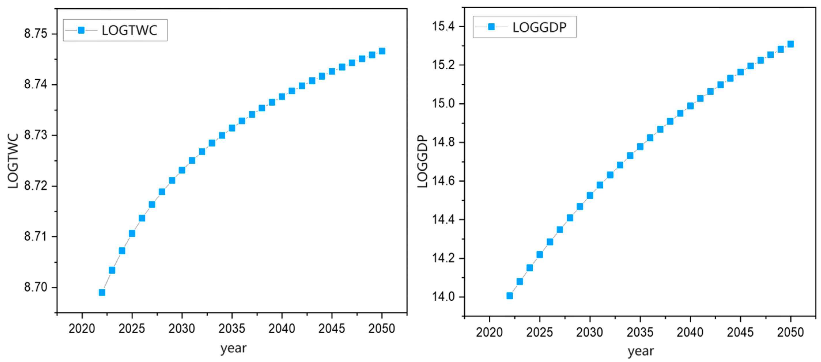
The VAR model predicted the changes in GDP and TWC of 2023–2050 (see Figure 5). From 2023 to 2050, TWC exhibited a gradual upward trend. Similarly, GDP followed a similar trend, showing continuous growth, albeit at a slower pace.

3.4. Water Overload Status Results

Considering the sustainable water resources management, we calculated the water environmental pressure index and the pressure index of water resources. By combining these indices, we derived the comprehensive water overload state index.
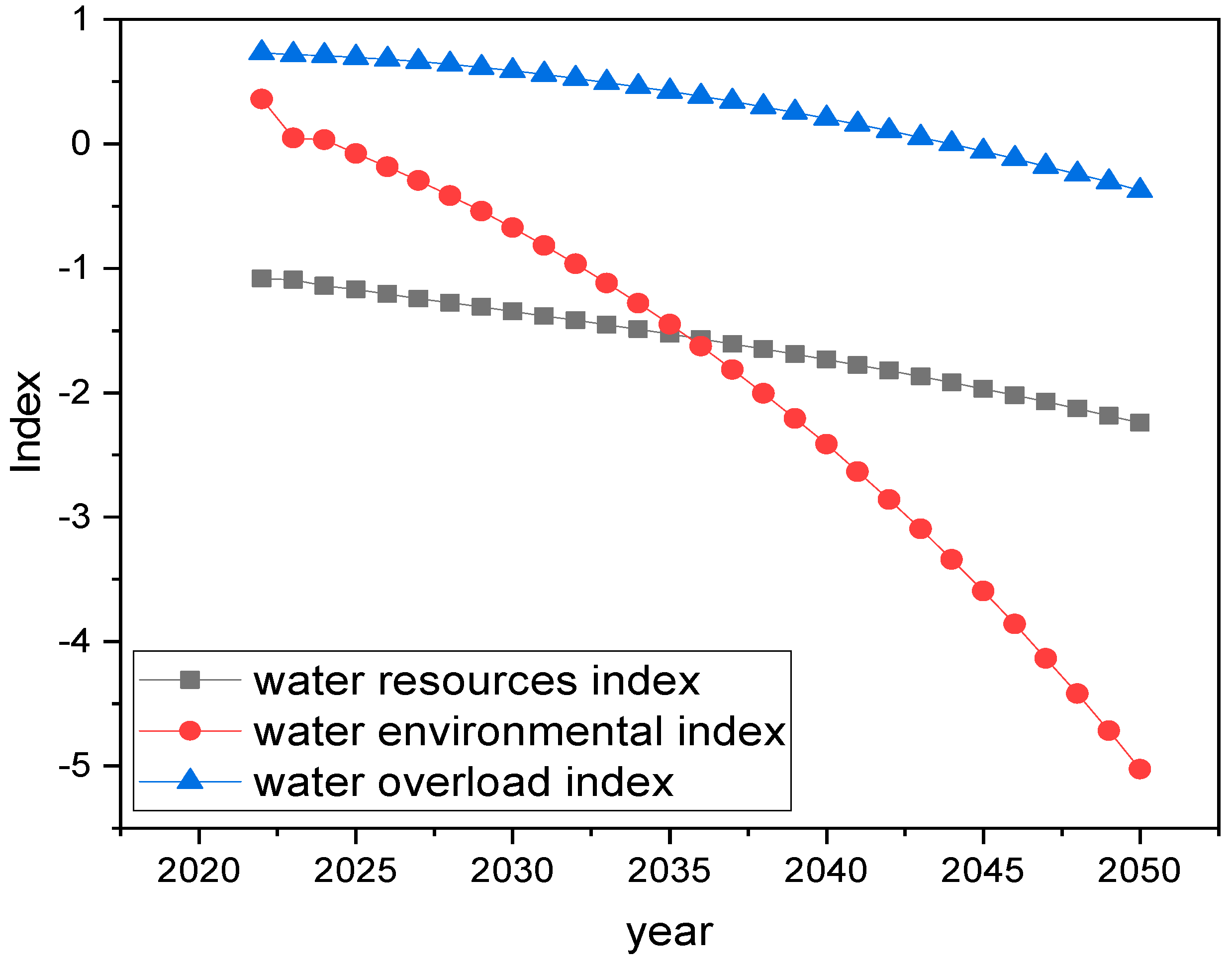
Figure 6 illustrates that the overload index displays a nearly linear decrease starting from the year 2023. The water pressure index was calculated by TWC and population. The water environmental index was calculated by TWC and the environmental indicators. Both the water environment pressure and water resources pressure indices exhibited similar trends, indicating that the status of China’s water resources was not optimistic, considering both the total amount and the development of the water environment.
However, it can be observed that the water environment index declines at the fastest rate between 2023 and 2050, while the water overload index and water resources index decrease at a slower pace, maintaining consistent levels of decline.

4. Conclusions and Recommendations

Using the time series data of GDP and water consumption from 2001 to 2022, a VAR model was established between GDP and TWC, and their co-integration relationship was tested. The dynamic interaction between GDP and TWC was analyzed using the generalized impulse response function and predictive variance, and the VAR model was applied to forecast the water consumption trends from 2023 to 2050.
The findings are as follows: (1) Over the study period, there existed a cointegration between China’s economic growth and TWC. However, TWC continued to demonstrate a notable increasing trend. The impact of GDP growth in curbing water resource consumption was not sufficiently evident. (2) The aggregated effect of GDP to TWC per capita was positive, and likewise, the aggregated effect of TWC to GDP was also positive. (3) GDP is a significant factor for predicting the variance of water resource use, whereas water use contributed less to the forecasted variance of economic growth. It is crucial to address the increase in TWC triggered by economic development and carefully consider the potential adverse effects of water shortages on economic growth. (4) According to the GCT results, the p-value of GDP to TWC was 0.0989. GDP did not serve as the granger cause of TWC, and the rapid growth of GDP significantly promoted the utilization of water resources, resulting in an increasing quantity of water use. (5) The water overload state index showed a declining trend between 2023 and 2050, implying a sustained improvement in China’s water overload condition.
Based on the research findings, we recommend that the government adopt the following policy measures to achieve the sustainable management of water resources and the sustained economic prosperity.
Develop a comprehensive plan for the sustainable development of water resources: The government should carry out a comprehensive water resource management plan, with clear objectives and measures to ensure efficient use and equitable distribution of water resources.
Encourage the promotion of water-saving technologies and awareness: The government should encourage businesses and individuals to adopt water-saving technologies and measures while also raising public awareness about the importance of water conservation through education and campaigns.
Enhance water resource regulation and enforcement: The government ought to enhance water resources regulation and establish a sound enforcement system to crack down on illegal water extraction and water pollution.
In conclusion, prioritizing water resource management will lead to a win–win situation for both ecological balance and economic development. This approach will have a positive and extensive effects on China’s environmental protection and economic growth.

Author Contributions

S.W.: data curation, formal analysis, and writing—original draft. S.W., J.L. and A.Z.: investigations. J.L. and A.Z.: writing—review and funding acquisition. S.W., Z.S. and A.Z.: writing—review and editing. All authors have read and agreed to the published version of the manuscript.

Funding

This research was funded by the National Natural Science Foundations of China (72103022, 72174111), the Youth Foundation in the Jiangsu Province of China (BK20220205), the Education Department and Natural Science Foundation of Hunan Province (21B0583, 2022JJ40137), and the China Postdoctoral Science Foundation (2020TQ0048, 2021M700460, 2022M710421).

Data Availability Statement

Data supporting the findings of this study are available from the corresponding author upon request.

Acknowledgments

The authors are grateful to the anonymous reviewers for their comments and suggestions which contributed to the further improvement of this paper.

Conflicts of Interest

The authors declare no conflicts of interest.

Abbreviations

In this manuscript, the following abbreviations are used:
VARVector autoregressive
GDPGross Domestic Product
TDCATime difference correlation analysis
TDCCTime difference correlation coefficient
OLSOrdinary least square
STFsSewage treatment facilities
CSYChina Statistical Yearbook
ADFAugmented Dickey–Fuller
TWCTotal water consumption
GCTGranger Causality Test

References

  1. Dolan, F.; Lamontagne, J.; Link, R.; Hejazi, M.; Reed, P.; Edmonds, J. Evaluating the economic impact of water scarcity in a changing world. Nat. Commun. 2021, 12, 1915. [Google Scholar] [CrossRef] [PubMed]
  2. Lu, Q.; Liu, F.; Li, Y.; Wang, D. Study on the Relationship between Water Resources Utilization and Economic Growth in Tarim River basin from the Perspective of Water Footprint. Water 2022, 14, 1655. [Google Scholar] [CrossRef]
  3. NBS. Statistical Communiqué of the People’s Republic of China on the 2021 National Economic and Social Development; National Bureau of Statistics: Beijing, China, 2022. [Google Scholar]
  4. Wang, Q.; Su, M. The effects of urbanization and industrialization on decoupling economic growth from carbon emission–a case study of China. Sustain. Cities Soc. 2019, 51, 101758. [Google Scholar] [CrossRef]
  5. Song, M.L.; Tao, W.L.; Shang, Y.P.; Zhao, X. Spatiotemporal characteristics and influencing factors of China’s urban water resource utilization efficiency from the perspective of sustainable development. J. Clean. Prod. 2022, 338, 130649. [Google Scholar] [CrossRef]
  6. Cai, B.; Guo, M. Exploring the drivers of quantity- and quality-related water scarcity due to trade for each province in China. J. Environ. Manag. 2023, 333, 117423. [Google Scholar] [CrossRef]
  7. Sun, Y.; Liu, N.; Shang, J.; Zhang, J. Sustainable utilization of water resources in China: A system dynamics model. J. Clean. Prod. 2017, 142, 613–625. [Google Scholar] [CrossRef]
  8. The Ministry of Ecology and Environment, P.R.C. Annual Bulletin of China’s Ecology and Environment. 2020. Available online: http://www.cnemc.cn/jcbg/zghjzkgb/ (accessed on 31 May 2023).
  9. Tao, T.; Xin, K. A sustainable plan for China’s drinking water: Tackling pollution and using different grades of water for different tasks is more efficient than making all water potable. Nature 2014, 511, 527–529. [Google Scholar] [CrossRef] [PubMed]
  10. Wang, Q.; Jiang, R.; Li, R.R. Decoupling analysis of economic growth from water use in City: A case study of Beijing, Shanghai, and Guangzhou of China. Sustain. Cities Soc. 2018, 41, 86–94. [Google Scholar] [CrossRef]
  11. Cicchetti, C.J.; Smith, V.K.; Carson, J. Economic-analysis of water-resources investment and regional economic growth. Water Resour. Res. 1975, 11, 1–6. [Google Scholar] [CrossRef]
  12. Hayat, A.; Tahir, M. Foreign direct investment, natural resources and economic growth: A threshold model approach. J. Econ. Stud. 2021, 48, 929–944. [Google Scholar] [CrossRef]
  13. Howe, C.W. Water resources and regional economic growth in united-states, 1950–1960. South. Econ. J. 1968, 34, 477–489. [Google Scholar] [CrossRef]
  14. Rosa, L.; Rulli, M.C.; Davis, K.F.; Chiarelli, D.D.; Passera, C.; D’Odorico, P. Closing the yield gap while ensuring water sustainability. Environ. Res. Lett. 2018, 13, 104002. [Google Scholar] [CrossRef]
  15. Montoya, M.A.; Allegretti, G.; Bertussi, L.A.S.; Talamini, E. Domestic and foreign decoupling of economic growth and water consumption and its driving factors in the Brazilian economy. Ecol. Econ. 2023, 206, 107737. [Google Scholar] [CrossRef]
  16. Wang, Q.; Wang, X. Moving to economic growth without water demand growth—A decomposition analysis of decoupling from economic growth and water use in 31 provinces of China. Sci. Total Environ. 2020, 726, 138362. [Google Scholar] [CrossRef] [PubMed]
  17. Distefano, T.; Kelly, S. Are we in deep water? Water scarcity and its limits to economic growth. Ecol. Econ. 2017, 142, 130–147. [Google Scholar] [CrossRef]
  18. Russ, J. Water runoff and economic activity: The impact of water supply shocks on growth. J. Environ. Econ. Manag. 2020, 101, 102322. [Google Scholar] [CrossRef]
  19. de Amorim, W.S.; Valduga, I.B.; Ribeiro, J.M.P.; Guazzelli Williamson, V.; Krauser, G.E.; Magtoto, M.K.; Guerra, J. The nexus between water, energy, and food in the context of the global risks: An analysis of the interactions between food, water, and energy security. Environ. Impact Assess. 2018, 72, 1–11. [Google Scholar] [CrossRef]
  20. Jin, W.; Zhang, H.Q.; Liu, S.S.; Zhang, H.B. Technological innovation, environmental regulation, and green total factor efficiency of industrial water resources. J. Clean. Prod. 2019, 211, 61–69. [Google Scholar] [CrossRef]
  21. Wada, Y.; Florke, M.; Hanasaki, N.; Eisner, S.; Fischer, G.; Tramberend, S.; Satoh, Y.; van Vliet, M.T.H.; Yillia, P.; Ringler, C.; et al. Modeling global water use for the 21st century: The Water Futures and Solutions (WFaS) initiative and its approaches. Geosci. Model Dev. 2016, 9, 175–222. [Google Scholar] [CrossRef]
  22. Alrwis, K.N.; Ghanem, A.M.; Alnashwan, O.S.; Al Duwais, A.A.M.; Alaagib, S.A.B.; Aldawdahi, N.M. Measuring the impact of water scarcity on agricultural economic development in Saudi Arabia. Saudi J. Biol. Sci. 2021, 28, 191–195. [Google Scholar] [CrossRef] [PubMed]
  23. Zhao, X.; Fan, X.; Liang, J. Kuznets type relationship between water use and economic growth in China. J. Clean. Prod. 2017, 168, 1091–1100. [Google Scholar] [CrossRef]
  24. Zhang, Y.; Gu, A.; Pan, B.L. Relationship between industrial water consumption and economic growth in China based on environmental Kuznets curve. Energy Procedia 2017, 105, 3557–3564. [Google Scholar] [CrossRef]
  25. Hao, Y.; Hu, X.L.; Chen, H.Y. On the relationship between water use and economic growth in China: New evidence from simultaneous equation model analysis. J. Clean. Prod. 2019, 235, 953–965. [Google Scholar] [CrossRef]
  26. Sims, C. Macroeconomics and Reality. Econometrica 1980, 48, 1–47. [Google Scholar] [CrossRef]
  27. Kang, S.H.; Islam, F.; Tiwari, A.K. The dynamic relationships among CO2 emissions, renewable and non-renewable energy sources, and economic growth in India: Evidence from time-varying Bayesian VAR model. Struct. Chang. Econ. D 2019, 50, 90–101. [Google Scholar] [CrossRef]
  28. Corradini, C. Local institutional quality and economic growth: A panel-VAR analysis of Italian NUTS-3 regions. Econ. Lett. 2021, 198, 109659. [Google Scholar] [CrossRef]
  29. Aslan, A.; Ocal, O.; Ozsolak, B.; Ozturk, I. Renewable energy and economic growth relationship under the oil reserve ownership: Evidence from panel VAR approach. Renew. Energy 2022, 188, 402–410. [Google Scholar] [CrossRef]
  30. Xiang, X.J.; Li, Q.; Khan, S.; Khalaf, O.I. Urban water resource management for sustainable environment planning using artificial intelligence techniques. Environ. Impact Assess. 2021, 86, 106515. [Google Scholar] [CrossRef]
  31. Schewe, J.; Heinke, J.; Gerten, D.; Haddeland, I.; Arnell, N.W.; Clark, D.B.; Dankers, R.; Eisner, S.; Fekete, B.M.; Colon-Gonzalez, F.J.; et al. Multimodel assessment of water scarcity under climate change. Proc. Natl. Acad. Sci. USA 2014, 111, 3245–3250. [Google Scholar] [CrossRef] [PubMed]
  32. Goelman, G.; Dan, R.; Ruzicka, F.; Bezdicek, O.; Ruzicka, E.; Roth, J.; Vymazal, J.; Jech, R. Frequency-phase analysis of resting-state functional MRI. Sci. Rep. 2017, 7, 43743. [Google Scholar] [CrossRef] [PubMed]
  33. Grizzetti, B.; Lanzanova, D.; Liquete, C.; Reynaud, A.; Cardoso, A.C. Assessing water ecosystem services for water resource management. Environ. Sci. Policy 2016, 61, 194–203. [Google Scholar] [CrossRef]
  34. Jose Moises, D.; Kunguma, O. Improving flood early warning systems in Kabbe, Namibia: A situational analysis approach. Int. J. Disaster Risk Reduct. 2023, 93, 103765. [Google Scholar] [CrossRef]
  35. Liu, M.; Wei, J.; Wang, G.; Wang, F. Water resources stress assessment and risk early warning–a case of Hebei Province China. Ecol. Indic. 2017, 73, 358–368. [Google Scholar] [CrossRef]
  36. Rød, E.G.; Gåsste, T.; Hegre, H. A review and comparison of conflict early warning systems. Int. J. Forecast. 2023, 40, 96–112. [Google Scholar] [CrossRef]
  37. The Ministry of Water Resources, P.R.C. China Water Resources Bulletin. 2022. Available online: http://www.mwr.gov.cn/zzsc/tjgb/szygb/2022/mobile/index.html (accessed on 15 September 2023).
  38. Wang, Z.; Xu, D.; Peng, D.; Zhang, X. Future climate change would intensify the water resources supply-demand pressure of afforestation in inner Mongolia, China. J. Clean. Prod. 2023, 407, 137145. [Google Scholar] [CrossRef]
  39. Li, D.; Zuo, Q.; Zhang, Z. A new assessment method of sustainable water resources utilization considering fairness-efficiency-security: A case study of 31 provinces and cities in China. Sustain. Cities Soc. 2022, 81, 103839. [Google Scholar] [CrossRef]
  40. Meo, M.S.; Sabir, S.A.; Arain, H.; Nazar, R. Water resources and tourism development in South Asia: An application of dynamic common correlated effect (DCCE) model. Environ. Sci. Pollut. Res. 2020, 27, 19678–19687. [Google Scholar] [CrossRef] [PubMed]
  41. Zhou, A.H.; Xin, L.; Li, J. Assessing the impact of the carbon market on the improvement of China’s energy and carbon emission performance. Energy 2022, 258, 124789. [Google Scholar] [CrossRef]
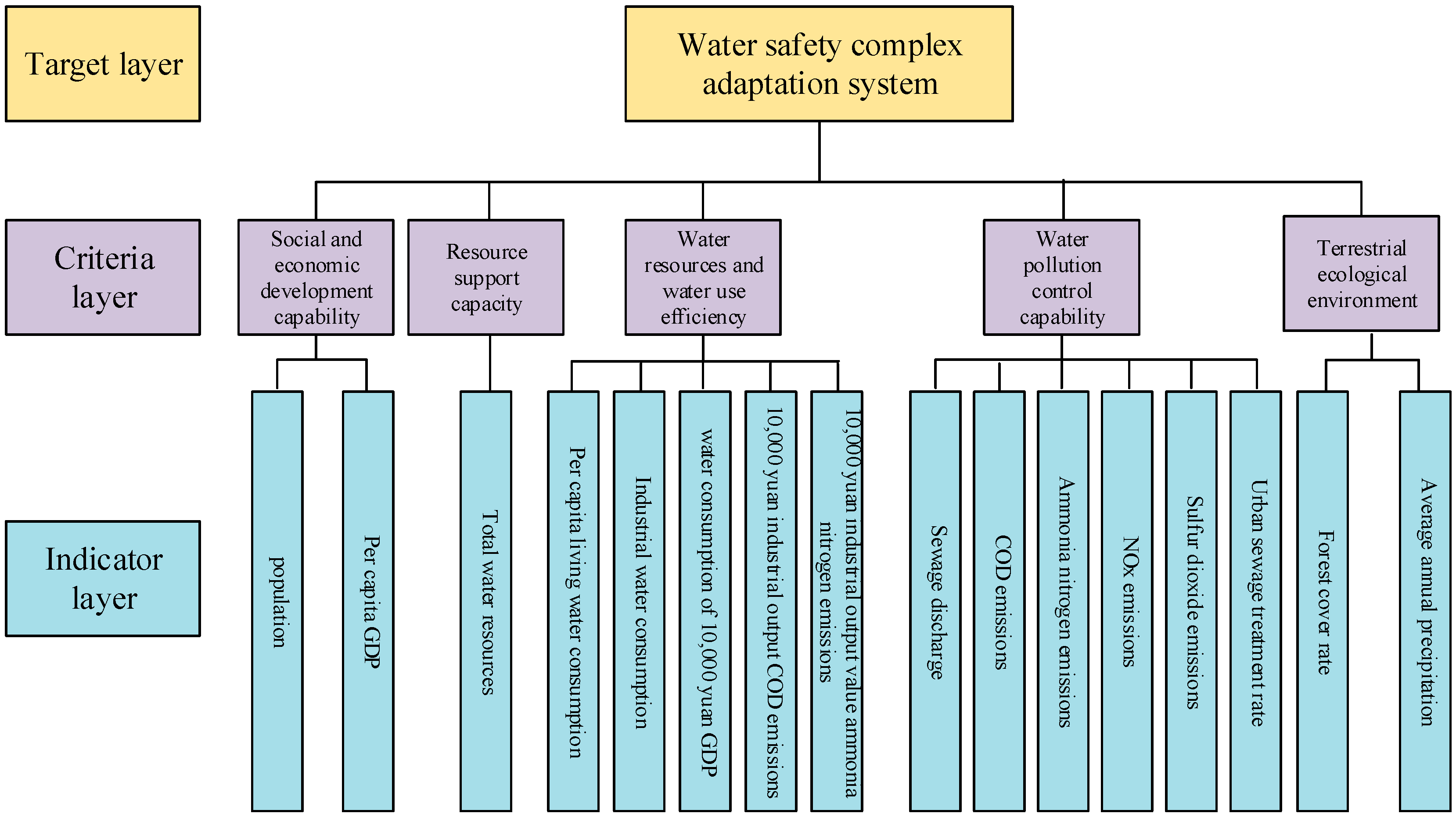
Figure 1. Early warning indicator hierarchy model.
Water 16 01325 g001
Figure 2. Unit circle test diagram.
Water 16 01325 g002
Figure 3. Impulse response function graph of GDP and TWC.
Water 16 01325 g003
Figure 4. Variance decomposition.
Water 16 01325 g004
Figure 5. Prediction of 2023–2050 based on the VAR model.
Water 16 01325 g005
Figure 6. Prediction of water resources, water environment, and water overload pressure index: 2023–2050.
Water 16 01325 g006
Table 1. Early warning indicator system construction.
NumberIndicatorIndicator
Classification
NumberIndicatorIndicator
Classification
T1Total water resources/100 million m3Internal systemT14NOx emissions/tonsInternal system
T2Total water consumption/100 million m3Internal systemT15Ammonia nitrogen emissions/tonsInternal system
T3Industrial water consumption/100 million m3Internal systemT16Total industrial exhaust emissions/billion m3Internal system
T4Per capita GDP/CNY 10,000External systemT17Population/millionInternal system
T5water consumption of CNY 10,000 GDP/m3Internal and external systemT18Exhaust gas treatment facilities/TaiInternal system
T6Per capita living water consumption/m3Internal systemT19CNY 10,000 industrial output COD emissions/tonsInternal and external system
T7COD emissions/tonsInternal systemT20Power generation/billion kWhExternal system
T8Ammonia nitrogen emissions/tonsInternal systemT21The difference in the number of units of STFs per unit/TaiInternal system
T9Sewage discharge/tonsInternal systemT22Forest cover rate/%Internal system
T10CNY 10,000 GDP sewage discharge/tonsInternal and external systemT23The difference in the unit GDP exhaust gas treatment facilities/TaiInternal system
T11Sewage treatment facilities/TaiInternal systemT24Power generation difference/billion kwhInternal system
T12Urban sewage treatment rate/%Internal and external systemT25CNY 10,000 industrial output value ammonia nitrogen emissions/tonsInternal and external system
T13Sulfur dioxide emissions/tonsInternal systemT26Average annual precipitation/mmExternal system
Table 2. Variable ADF test results.
VariablesADF Statistics(c, t, k)SignificantConclusions
I−1.4173(c, 0, 0)0.5542unstable
LOGI−1.4190(c, 0, 0)0.5534unstable
DLOGI−4.3906(c, 0, 0)0.0029stable
DDLOGI−8.6653(c, 0, 0)0.0000stable
J3.6281(c, 0, 0)1.0000unstable
LOGJ−3.2498(c, 0, 0)0.0311stable
DLOGJ−2.4218(c, 0, 0)0.1486unstable
DDLOGJ−5.7211(c, 0, 0)0.0002stable
Table 3. Cointegration test results.
RankParamsLLEigenvalueTrace StatisticCritical Value
02−370.9920 18.921915.4100
15−361.80700.58300.5510 *3.7600
26−361.53100.0259
Note: * Refers to the existence of a cointegration relationship.
Table 4. Results of lag order selection for the VAR model.
CategoriesLag PhaseLogLHQSCFPELRAIC
GDP and TWC031.7167−3.4863−3.39800.0001NA−3.496090
189.9609−9.8485 *−9.5836 *1.77 × 10−7 *95.9316 *−9.877761 *
291.9565−9.5932−9.15182.31 × 10−72.8173−9.6419
394.5015−9.4025−8.78462.93 × 10−72.9941−9.4707
499.2552−9.4717−8.67723.07 × 10−74.4740−9.5594
599.9781−9.0667−8.09565.82 × 10−70.5102−9.1738
Note: * represents the optimal lag order.
Table 5. Overall test results of the VAR model.
Statistics ValueEquation (5) Results
Residual Covariance (+degrees of freedom)3.14 × 10⁻⁷
Residual Covariance2.30 × 10−7
Log—Likelihood Estimation100.8821
Akaike Information Criterion−9.0363
Schwarz Criterion−8.7379
Table 6. Stability test results.
Equation (5)
RootModule
0.96310.9631
0.80170.8017
Table 7. Results of GCT.
Null HypothesisSamplesF Statisticp ValuesYes/No
LNJ does not Granger Cause LNI160.452480.8123No
LNI does not Granger Cause LNJ165.332240.0989Yes
Disclaimer/Publisher’s Note: The statements, opinions and data contained in all publications are solely those of the individual author(s) and contributor(s) and not of MDPI and/or the editor(s). MDPI and/or the editor(s) disclaim responsibility for any injury to people or property resulting from any ideas, methods, instructions or products referred to in the content.