Assessing Pipe Condition in Water Distribution Networks

Abstract

The condition assessment of water distribution pipes is of utmost importance for the prioritization of rehabilitation interventions. However, the application of available methodologies for condition assessment by water utilities with limited human, technological and financial resources is becoming increasingly complex. The current paper aims at the development and application of a methodology for the prediction of the physical condition of water distribution pipes without the need for visual inspection. The methodology includes the development and application of three different algorithms (heuristic, linear regression and support vector regression). The methodology is applied to a water distribution network located in the Algarve region, Portugal. The results obtained from each algorithm are compared with a well-known performance indicator, the ratio of useful life, and present significant differences in its overall pipe condition classification. Results have demonstrated the following: the ratio of useful life tends to distribute pipe classification more equally in the three classes (i.e., good, average and unsatisfactory); the heuristic algorithm classifies most pipes as average condition; and the linear regression algorithm classifies with unsatisfactory conditions. The support vector regression algorithm stands out as the main classifier for identifying pipes in good condition when compared to other algorithms.

1. Introduction

Water distribution networks inevitably undergo a degradation process, leading to the occurrence of multiple anomalies, such as leaks, bursts, blockages, entrapped air, unsealed valves and water contamination [1]. Numerous utilities are challenged by the urgent need to replace their most degraded assets to meet existing and future requirements. This aspect is more significant in developed countries, where infrastructures were built decades ago and, often, little investment has been made in their renovation [2]. The assessment of the physical condition of water pipes is an important process of infrastructure asset management (IAM), which corresponds to a set of processes that can be applied by water utilities to balance the three dimensions of analysis in the long-term—cost, risk and performance [3]. An efficient IAM aims to provide an asset management plan, allowing for the minimization of the life-cycle costs by lowering renewal costs, identifying the necessary measures for optimized resource allocation and prioritizing the necessary interventions [4].

A comprehensive methodology for IAM to be applied at the three decision levels—strategic, tactical and operational—for asset management is needed [5]. Condition assessment is integrated into IAM in the process of asset performance evaluation. Different methods can be considered for the condition assessment of water distribution pipes, such as direct or indirect methods [6]. Direct condition assessment methods require the inspection of the pipe, which can be intrusive (i.e., requiring access to the interior of the pipe with or without interruption of the supply service) and non-intrusive methods (i.e., not requiring access to the interior of the pipe, but often requiring excavation) [7]. Indirect condition methods include the collection and analysis of the assets’ physical characteristics (e.g., pipe material, diameter, installation date), failure history (e.g., number of busts per year, burst location) and the previous inspection information to estimate the current physical condition [8,9]. These methods can be classified in two categories—environmental (i.e., involving the surveying of soil and water chemistry) and operational (i.e., involving leak/burst history, pipe material embedment, coating or linings calculation)—and aim to analyze trends and changes in the system to provide information on the condition of assets [10,11]. The main advantage of indirect condition assessment methods compared to direct methods is that inspection is not necessary in most cases. As a result, the interruption of the service is avoided, as is the associated cost [11].

The development of indirect condition assessment methods is often based on the known relationships between deterioration and the factors that affect the physical condition of buried pipes. These factors can be divided as follows [12]: (i) physical factors, which are factors related to intrinsic pipe properties, such as pipe material, age, nominal diameter, wall thickness, pipe lining and coating, type of joints and manufacturing process; (ii) environmental factors that are related to the environment in which the pipe is located, such as soil pH, groundwater level, pipe location in relation to traffic, seismic activity, stray electric currents, trench backfill material, pipe bedding, installation practices and underground disturbances; and (iii) operational factors that are associated with the operating conditions of the pipe, such as water quality, water pressure, backflow potential, flow velocity and operational and maintenance (O and M) practices. A burst in a water distribution pipe, if not caused by third parties, can be attributed to pipe deterioration and interpreted as a sign of decreased physical condition. This occurrence can be due to a single influencing factor or a combination. While the factors that contribute to the deterioration of water distribution pipes are known, the relative influence of each factor is widely discussed [13]. As a result, even though research has proven the existence of failure mechanisms, the uncertainty associated with the exact relationship between factors is still the focus of several studies.

Several algorithms have been developed to assess and predict the physical condition of water distribution pipes. These vary from basic techniques that rely on limited data to highly precise prediction models leveraging the latest advancements in machine learning. The use of key performance indicators to assess the asset condition is one of the most used approaches in Portugal, especially the use of the Infrastructure Value Index (IVI). This index was firstly proposed by [14] and is defined as the ratio between the current value of the infrastructure and its replacement cost:

$$IVI(t)=\frac{{\displaystyle \sum _{i=1}^{n_i}\left(r{c}_{i,t}\cdot \frac{ru{l}_{i,t}}{eu{l}_i}\right)}}{{\displaystyle \sum _{i=1}^{n_i}r{c}_{i,t}}}$$

(1)

in which IVI (t) is the infrastructure value index at time t, rc_i,t is the replacement cost of asset i at time t, rul_i,t is the residual useful life of asset i at time t, eul_i is the expected useful life of asset i and n_i is the total number of assets. This index aims at assisting long-term planning of urban water assets; however, it can also represent the current age and the intervention needs of a given infrastructure. When calculating IVI at the asset level, the key performance indicator represents the ratio of useful life (RUL) of each pipe, corresponding to the ratio between the asset age and its useful life.

Other algorithms include deterministic, heuristic or machine learning techniques. Deterministic techniques are commonly used when a non-random relationship between variables is considered. A well-known study that has developed deterministic algorithms is [15]. This study estimated the remaining useful life for gray cast iron water pipes, using a total of 29 parameters. These algorithms are easy to apply and understand; however, they are inappropriate in scenarios where the risk of an event is a relevant criterion for decision-making, e.g., seismic risk and vulnerability studies [16]. Heuristic techniques are more common when the influencing factors are not well understood, allowing for the development of algorithms through subjective opinions from experienced field engineers and experts [17]. Ref. [18] proposed a pipe condition rank method using fuzzy PROMETHEE II. This model was applied to eight pipe samples and the results ranked each pipe by the highest to lowest breakage risk. These algorithms are developed with limited or no pipe data; however, results are highly influenced by the opinion of the expert groups. Finally, new algorithms that rely on machine learning techniques have been proposed, including generalized linear models, deep learning, decision trees, random forests, XGBoost, AdaBoost and support vector machines [19]. Ref. [20] studied different machine learning algorithms, such as random forests, decision trees, neural networks and support vector machines to accurately locate water leaks in water distribution systems.

These algorithms are very challenging to implement in water distribution systems, given the limited infrastructure data. In Portugal, 51 out of 136 water utilities do not have any form of formal inventory of assets, including information related to pipe location and historical data, and only 20 water utilities are reported to have any information regarding the condition of the assets [21]. Overall, there is an urgent need to address the gap between the condition assessment algorithms and the existing required resources in water utilities, namely, financial, human and technological. Thus, the main objective of this research is to develop a methodology to assess the physical condition of water distribution pipes based on three different algorithms and without the need for visual inspection or service interruption. The proposed methodology takes into consideration the knowledge gaps that Portuguese water utilities face, regarding the low infrastructure knowledge and the limitations of the current method used for indirect condition assessment (i.e., IVI). Three different algorithms are developed, compared and applied to assess the pipe physical condition of a Portuguese water distribution network, including heuristic, linear regression and support vector regression algorithms.

The paper is organized in five sections, including the current one. Section 2 presents the proposed methodology to assess the physical condition of water distribution pipes, describing the three algorithms. Section 3 presents the case study to which the methodology is applied and Section 4 shows, compares and discusses the condition assessment results. Lastly, Section 5 presents the main conclusions of this research and highlights foreseen future works.

2. Proposed Methodology

2.1. General Framework

The proposed methodology for assessing the physical condition of water distribution pipes is a three-step procedure:

(1)

Data collection and validation;

(2)

Algorithm development;

(3)

Condition assessment.

This methodology allows water utilities to efficiently assess the physical condition of their water distribution networks without the need for inspection or extensive field survey, which represents a less resource-consuming process. The application of this methodology also aims to contribute to the improvement of resource allocation and investment planning, resulting in the enhancement of the physical sustainability and integrity of water distribution networks.

The first step of the proposed methodology aims at collecting the factors that influence the physical condition of water pipes, which can be divided into three main categories: physical, operational and environmental. The collection of the failure history is also required to assess the physical condition of water pipes without inspection, including the type and date of bursts and their location. All collected data needs to be validated and checked for any inconsistencies (e.g., incorrect installation year of water pipes or inappropriate material choice for the nominal diameter). The most relevant factors that influence pipe deterioration are identified in the literature and summarized in

Table 1. Potential influencing factors of pipe deterioration.

Category	Factors
Physical	Pipe material, year of installation, nominal diameter, length, installation depth, wall thickness, Hagen Williams coefficient, cathodic protection, manufacturing process, location, laying conditions and number of households supplied.
Operational	Static pressure, pressure variance, water pH, chlorine levels, phosphate inhibitors, water temperature, water pressure and pressure surge allowance.
Environmental	Type of soil, groundwater level, soil pH, soil resistivity, soil density, backfill material, traffic intensity, wheel load ratio, soil aeration index, road surface type, external loads and ratio of horizontal to vertical pressure in the soil.
Failure history	Failure history, date of burst, corrosion depth, bursting tensile strength and ring modulus of rupture.

.

The second step of the proposed methodology is the development of different algorithms to assess the physical condition of water pipes, e.g., heuristic, linear regression and support vector regression. Heuristic algorithms rely on a theoretical framework for model construction, aiming at applying intuition to problem-solving and reducing the resources needed to achieve an adequate result. On the other hand, linear regression and support vector regression algorithms receive and analyze input data to predict output values within an acceptable range. The study of these two different algorithms allows us to identify their advantages and limitations and to compare the condition assessment results to ensure informed decision-making. A detailed description of each algorithm is presented in the following sections.

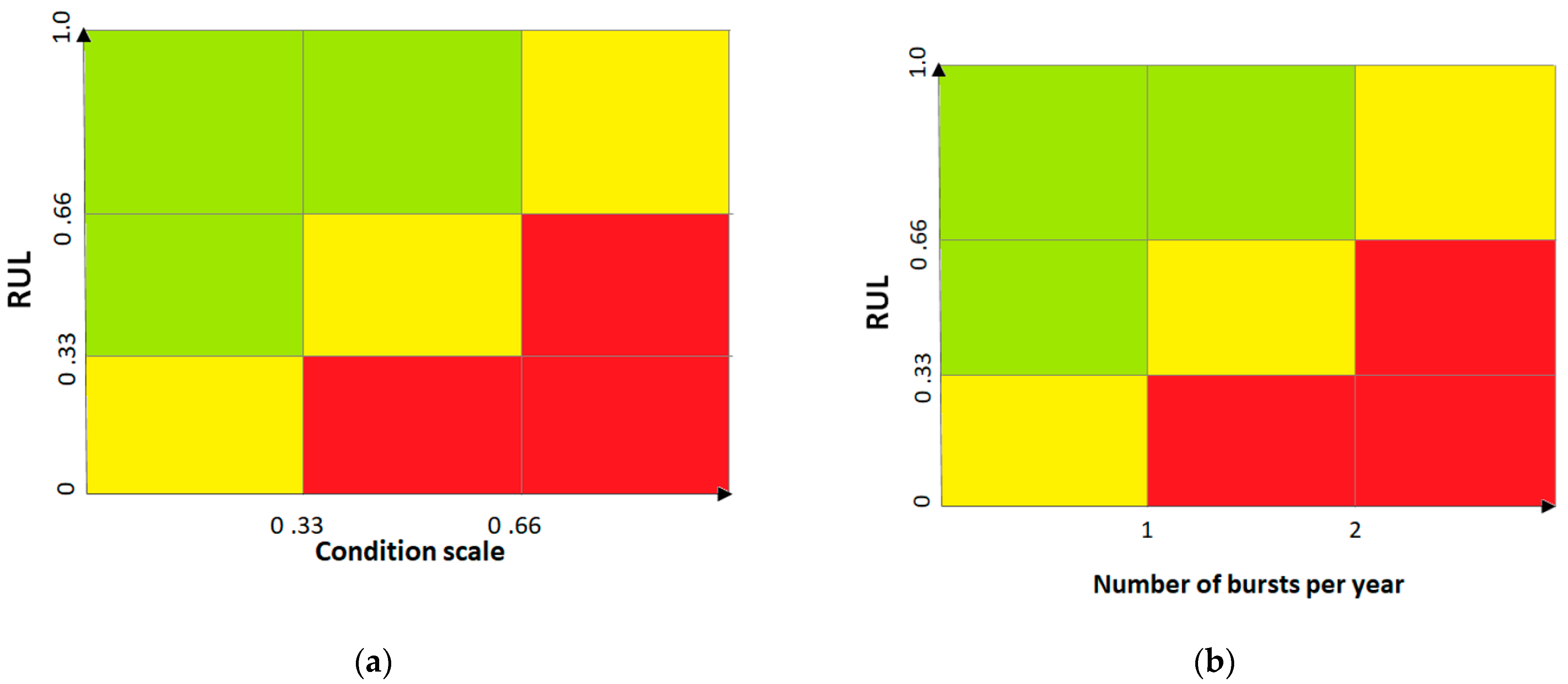
The third step of the proposed methodology aims at developing a comprehensive condition rating scale to interpret the algorithms’ results and to assess the physical condition of water distribution pipes. A condition matrix with three condition rating levels, namely good (represented by the green colour), average (represented by the yellow colour) and unsatisfactory (represented by the red colour), is developed.

Different condition matrices are developed for combining the algorithm results with the performance indicator of the ratio between the asset age and the useful life, designated as the Ratio of Useful Life (RUL). The idea behind the construction of these condition matrices is to combine a well-known performance indicator with data related to observations (e.g., pipe burst) made during the operation of the network. The RUL scale varies between zero and one, one being the value associated with newly installed pipes and zero being the value associated with pipes that have already reached their reference useful life and still remain in service. Three ranking levels equally divided are considered for the RUL scale.

The scale adopted for the algorithm results varies for each technique. In the heuristic algorithm, the proposed scale is similar to RUL with three ranking levels equally divided according to the interval of variation of the pipe condition model. The proposed condition matrix for the heuristic algorithm is presented in Figure 1a. For the remaining two algorithms (i.e., linear regression and support vector regression), the scale is based on the number of bursts during the observation period. This scale could vary with acceptable condition thresholds considered for each water utility, which in most cases depends on the available annual budget for interventions. Figure 1b illustrates a condition matrix for the two remaining algorithms, considering that zero bursts per year during the observation period (OP) are associated with pipes in good condition, with one burst for pipes in average condition and two bursts or more for pipes in unsatisfactory condition.

2.2. Heuristic Algorithm

The heuristic algorithm aims at developing condition models using weights for each factor that influences pipe deterioration calculated through a survey of experts in this field. The heuristic algorithm is composed of three main steps:

• Development of a survey on the influence of internal and external factors on pipe deterioration.
• Processing and analysis of the survey data and calculation of weighting factors.
• Development of condition models.

The first step aims at developing a survey to assess the importance of different factors on the physical condition (translated by the deterioration) of water distribution pipes, considering the following categories: (i) pipe characteristics and operating conditions; and (ii) external factors. The survey should be short, clear and unambiguous and the structure chosen should facilitate data collection. Experts should only answer questions regarding factors they are familiar with, avoiding the collection of guessing data. Additionally, the number of years of experience that experts have in the field is also collected to assess the perception that each experience group has of the influencing factors. In the developed survey, the influencing factors are evaluated on a scale from zero to five, in which zero means that the factor is irrelevant to pipe deterioration and five means that the factor is very relevant.

The second step aims at processing and analyzing the collected data from the surveys and calculating the weights that each factor has on physical condition. To calculate these weights, weighting methods are applied to assess different aspects of the collected data, namely the discrepancies in the average value (i.e., the use of the average and median values) or the overall confidence of experts in their perceptions (i.e., the bias of the number of replies for each factor). Furthermore, it should be noted that weights should range from zero to one and the total weight sum should be one.

The final step aims at developing the condition models with the calculated weighting factors. The construction of models should take into consideration the positive or negative relationship of each weighting factor with the physical condition of water distribution pipes. This means that special attention must be given to the variation of the influencing factor and their contribution to the condition grade, through the knowledge gathered by the literature review.

2.3. Linear Regression Algorithm

Linear regression assumes that pipe deterioration has a non-random relationship with network characteristics that yield pipe failure. These failures can only be detected by water utilities during a pipe inspection or when a burst occurs, which is the most common type of failure history, as direct action needs to be taken when detected. As a result, this algorithm uses failure history as a dependent variable and aims to construct models that estimate this theoretical failure considering different independent variables related to physical, operational and environmental factors. The steps that are needed to complete this algorithm are the following:

• Development of a correlation matrix between network characteristics (i.e., independent variables) and failure variables (i.e., dependent variables).
• Construction and assessment of linear regression models.
• Validation of regression models.

The first step aims at developing a correlation matrix with the dependent and independent variables. The independent variables are the characteristics of water distribution pipes (e.g., year of installation, material, nominal diameter) and the dependent variables are the failure history. Preferably, the collected variables should be quantitative; this operation might require the conversion of categorical variables to numerical values. The construction of the correlation matrix allows us to identify the highest-correlation coefficients that best describe the relationship between dependent and independent variables. The Spearman’s rank correlation coefficient is used to construct the correlation matrix, as it provides a nonparametric technique and measures the strength and direction of a non-monotonic relationship [22].

The second step consists of the construction of simple and multiple linear regression models and the assessment of the developed regression models through statistical analysis. Statistical analysis includes the calculation of the coefficient of determination for both simple (r-squared) and multiple regression analysis (adjusted r-squared) as well as the statistical significance of linear models by null hypothesis testing. The multicollinearity between explanatory variables (i.e., independent variables) is verified by the mathematical measurement of the variance inflation factor (VIF). Values higher than or equal to 10 are considered to have a high degree of multicollinearity and, therefore, are excluded from the models [23].

The third step corresponds to the validation of linear models by verifying the statistical dispersion of the collected data through the evaluation of the root mean square error, relative error and absolute error. The collected data must be divided into two subsets to carry out the validation: the training subset used for model construction, typically representing 80% of the whole dataset, and the validation subset used to validate the obtained results, representing the remaining 20% of the dataset. The goal of the validation subset is to perform cross-validation of the evaluated models and flag problems, such as overfitting and selection bias [24].

2.4. Support Vector Regression Algorithm

This subsection explores support vector regression (SVR) as an alternative to linear regression for predicting pipe failures. Unlike linear regression, which is based on a linear relationship between variables [25], SVR can effectively model non-linear and complex relationships [26] between network characteristics and failure occurrences. This characteristic makes SVR a potentially more suitable approach for scenarios where the deterioration process exhibits non-linear behavior, such as in aging pipe networks.

The objective of SVR is to find a hyperplane in the high-dimensional feature space that maximizes the margin between the hyperplane and the closest data points, also called support vectors, from each failure class:

$$w\phi (x)+b=0$$

(2)

in which $w\in {\Re }^d$ is the weight vector, φ(x) is the transformed input vector in the feature space and b is the bias term.

The process of finding the optimal hyperplane can be formulated as a convex optimization problem that minimizes the error of approximation. This minimization is also described as the ε-insensitive loss across all data points [26]. The ε-insensitive loss function penalizes deviations from the desired behavior and the model prediction for a certain input. Solving this optimization problem using appropriate algorithms allows us to obtain the optimal weight vector (w) and bias term (b) that define the decision function for classifying unseen data points. Prediction for a new data point involves projecting it into the high-dimensional feature space using the chosen kernel function and calculating the distance from its projection to the established hyperplane.

The SVR algorithm is applied to estimate the number of failures for each pipe by using the same network characteristics, as the ones used in linear regression. The classification of each pipe based on the number of failures is evaluated by using a confusion matrix, comparing the real number of failures with the estimated one. Furthermore, to compare the results with the linear regression algorithms, the determination coefficient is calculated.

3. Case Study

A water distribution network with a total length of approximately 85 km and serving 1787 houses with an annual water volume of 1,805,024 m³ is studied. This distribution system includes three pumping stations and four water storage tanks. The network is located in low-density residential housing and the domestic consumers correspond, mainly, to detached houses, which are mostly used in the summer season. Thus, this utility is characterized by seasonal water consumption with high outdoor water use in the summer and four to five times lower water consumption during the winter.

A total of 1666 distribution pipes comprise the network with different materials, such as polyvinyl chloride (PVC), asbestos cement (AC), ductile iron (DI), steel and high-density polyethylene (HDPE). The most predominant pipe material is PVC, corresponding to 53% of the total network, followed by AC (27%) and DI (17%) (Figure 2a). The nominal diameter of distribution pipes varies between 50 and 600 mm, with the most common pipes, those with small nominal diameters (i.e., less than 250 mm), representing more than 75% of the total distribution pipes (Figure 2b). The distribution network was initially constructed in 1972; however, the largest expansion of the network took place between 1982 and 1992, in which 50% of the pipes were installed (Figure 2c).

The studied distribution network presented 113 bursts during the observation period between February 2014 and February 2020. From a total of 113 bursts, 41 were classified as third-party interventions, while the remaining 72 bursts can be attributed to the natural process of pipe deterioration (2 of these bursts were not considered for further analysis due to being located in service connections). A total of 70 bursts, located in 49 different pipes, are considered for the present study.

4. Results

The proposed methodology is applied to the described case study to assess the physical condition of water distribution pipes, considering three different algorithms (i.e., heuristic, linear regression and support vector regression). A detailed description and discussion of the results are divided by the type of algorithm used and presented in the following sections.

4.1. Heuristic Algorithm

4.1.1. Development of a Survey on the Influence of Internal and External Factors on Pipe Deterioration

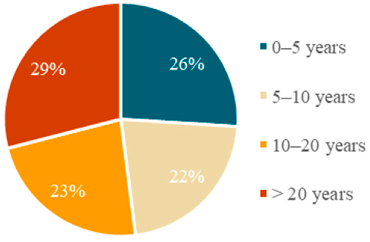
The perception of experts is collected through a survey, in which the influence of each factor already identified in Table 1 is evaluated. A total of 31 experts in the water supply sector, with professional careers of different maturity levels, were surveyed. All surveyed experts are engineers working for the public or private sector, including water utilities, academia and research. The distribution of their professional experience described by the duration of their professional career is presented in Figure 3. The number of experts in each experience group is similar, allowing us to obtain fairly distributed results throughout each group: eight experts with 0–5 years of experience (26%), seven experts with 5–10 years of experience (22%), seven experts with 10–20 years of experience (23%) and nine experts with more than 20 years of experience (29%).

4.1.2. Processing and Analysis of the Survey Data and Calculation of Weighting Factors

The processing and analysis of the survey results allows us to obtain quantitative weights for each influencing factor. The mathematical formulas used to obtain the weights are presented in

Table 2. Methods for obtaining factor weight attribution in the heuristic algorithm.

Factor Weight	Equation
Answer-based weights	$w_i=\frac{S_i}{{\displaystyle \sum _{i=1}^n{S}_i}}$
Number of replies and answer-based weights	$w_i=\frac{S_i\times A_i}{{\displaystyle \sum _{i=1}^n{S}_i\times A_i}}$
Median-based weights	$w_i=\frac{m_i}{{\displaystyle \sum _{i=1}^n{m}_i}}$
Number of replies and median-based weights	$w_i=\frac{m_i\times A_i}{{\displaystyle \sum _{i=1}^n{m}_i}\times A_i}$
Mean-based weights	$w_i=\frac{I_i}{{\displaystyle \sum _{i=1}^n{I}_i}}$
Number of replies and mean-based weights	$w_i=\frac{I_i\times A_i}{{\displaystyle \sum _{i=1}^n{I}_i\times A_i}}$

Notes: w_i is the weight of factor i; S_i is the sum of answers of factor i; n is the total number of influencing factors; A_i is the number of answers of factor i; m_i is the median value of factor i; and I_i is the average value of factor i.

. Each weight aims to value a certain aspect of the collected data that allows for the comparison of each factor’s influence. For example, the use of average- versus median-based weights allows us to evaluate the susceptibility to outliers in the collected data.

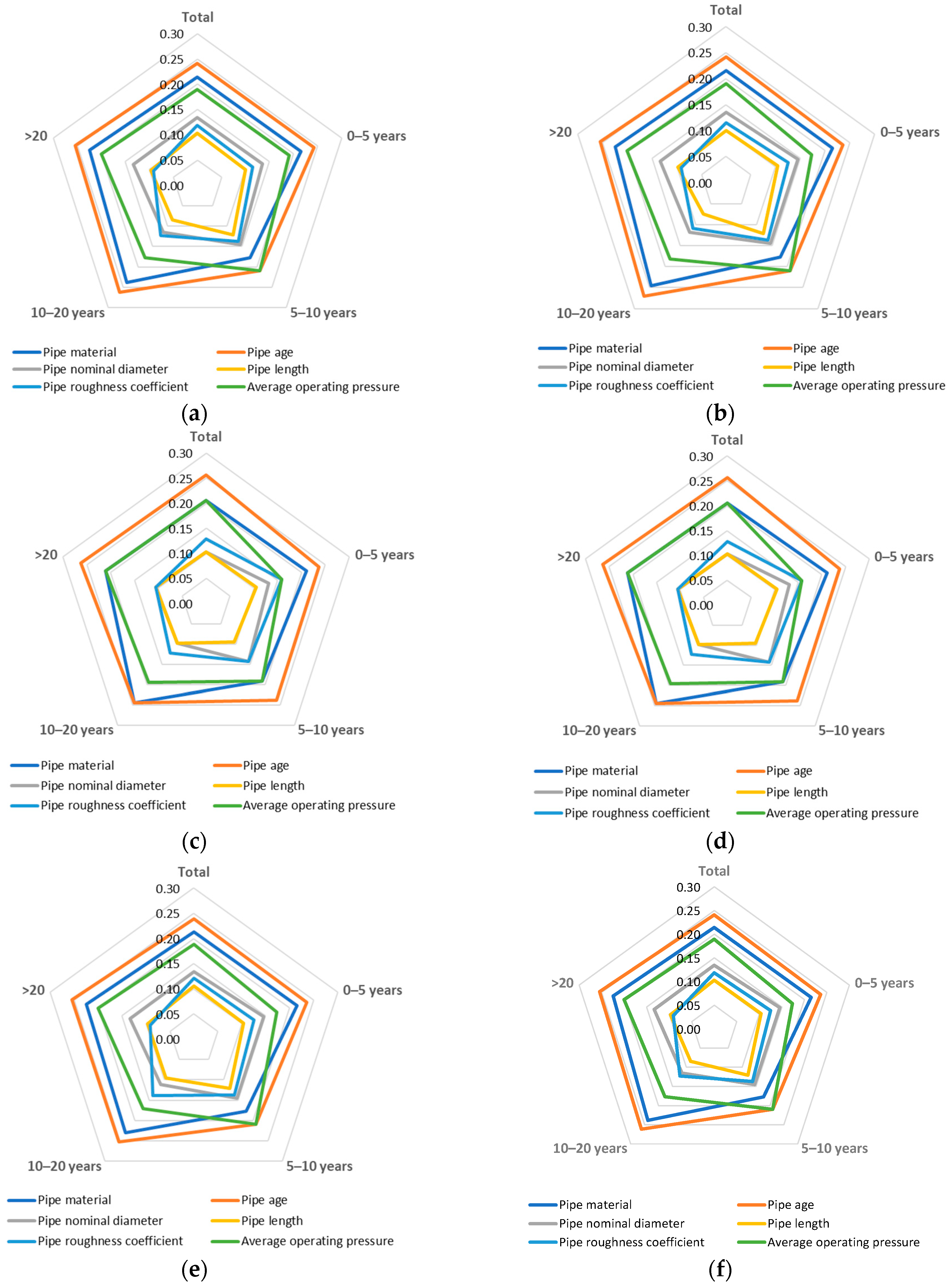
Since the available data in the case study does not exist for all considered factors (see Table 1), only six factors were analyzed, namely pipe material, pipe age, pipe nominal diameter, pipe length, pipe roughness coefficient and average operating pressure (considered the same as the static pressure for this study). The diagrams with the obtained weights for each of the six factors using the different mathematical formulations (Table 2) are presented in Figure 4. The vertices of the diagrams represent the weight attributed by each expert experience group.

Pipe age is the most relevant factor in pipe deterioration. However, the group with 5–10 years of experience also considers the average operating pressure of pipes as an equally important influencing factor of deterioration when using most weight formulas. On the other hand, the evaluation of the weight associated with each factor is very similar throughout experience groups with the order of most influential to least influential factors: age, material, average operating pressure, nominal diameter, roughness coefficient and length. Although some variation of this order can be identified, mainly in Figure 4e, the overall consensus of the experts remains.

Additionally, it can also be concluded that the order of influence in the factors does not change with the different weight calculation methods. Furthermore, the multiplication of the number of replies did not significantly change the results, which can be explained by the recommendation for experts to avoid guesswork in the survey leading to potential outliers in the answers. Nevertheless, when analyzing the weights attributed by expert experience groups, different perceptions arise. While all expert experience groups agree that pipe age is highly influential, the group with 10–20 years of experience concludes that pipe material and pipe age are highly influential, while the experts with more than 20 years of experience attribute a higher influence to average operating pressure than pipe material.

Table 3. Obtained weights using answer-based weights for the total expert group and the +20 expert group.

Factor	Answer-Based Weights and Total Expert Group	Answer-Based Weights and +20 Expert Group
Pipe age	0.2407	0.2546
Pipe material	0.2142	0.2242
Pipe nominal diameter	0.1345	0.1333
Pipe roughness coefficient	0.1186	0.0909
Pipe length	0.1027	0.0970
Average operating pressure	0.1893	0.2000

presents the results of the weight values using answer-based weights for the total expert group and the +20 expert group. These weights were considered for the subsequent analyses. Note that the summation of the weights equals 1.

4.1.3. Development of Condition Models

The development of a pipe condition model using the obtained weights requires the normalization of the properties of each pipe according to the following equation:

$$N_{n,i}=\frac{y_{n,i}-y_{\min ,i}}{y_{\max ,i}-y_{\min ,i}}\times w_i$$

(3)

in which N_n,i is the normalized and weighted influencing factor i for pipe n; y_n,I is the value of the influencing factor i for pipe n; y_min,i is the minimal value for the influencing factor i; y_max,i is the maximum value for the influencing factor i; w_i is the attributed weight for the influencing factor i.

Finally, the sum of the weighted variables of each factor results in a non-dimensional value of physical condition for each pipe as follows:

$$C_n={\displaystyle \sum _{i=1}^n{N}_{n,i}}$$

(4)

in which C_n is the condition value for the pipe n.

It should be noted that influencing factors do not present the same relationship (positive or negative) with pipe physical condition; thus, special attention must be given to the variation of the influencing factors and their contribution to the condition grade through the knowledge gathered by the literature review.

The pipe condition model is applied to the described case study considering the total expert knowledge (i.e., 31 experts) and the most experienced experts (i.e., over 20 years of experience) and using the answer-based weights. The condition scale presented in Figure 1a is used to classify the physical condition of pipes as good, average and unsatisfactory. The obtained results are quite similar for both categories of expert groups, classifying most of the network with an average condition (

Table 4. Pipe condition results using a heuristic algorithm and considering answer-based weights for the total expert group and +20 expert group.

Condition Grade	Answer-Based Weights and Total Expert Group		Answer-Based Weights and +20 Expert Group
	Number of Pipes	Relative Frequency (%)	Number of Pipes	Relative Frequency (%)
Good	370	22.21%	201	12.06%
Average	994	59.66%	1165	69.93%
Unsatisfactory	302	18.13%	300	18.01%
Total	1666	100%	1666	100%

).

Figure 5 and Figure 6 present the pipe material and pipe age distribution for the three condition grades (i.e., good, average and unsatisfactory), respectively. The majority of the pipes classified as unsatisfactory condition are made of AC and PVC, which are the materials mostly installed between 1970 and 2000 (Figure 5). In terms of pipe age distribution, there is a tendency for more recent pipes to be classified as good condition (almost 50% of the pipes present an age between 0 and 20 years), followed by pipes classified as average condition and with an intermediate age (i.e., 62% of the pipes present an age between 20 and 30 years). Finally, the majority of the older pipes are classified as unsatisfactory condition, representing 75% of pipes with an age higher than 30 years (Figure 6).

4.2. Linear Regression Algorithm

4.2.1. Development of a Correlation Matrix between Network Characteristics and Failure Variables

As mentioned in the proposed methodology, this algorithm aims to use network properties as independent variables to model the failure history of the network (e.g., the number of bursts, rate of bursts, number of bursts per year). The regression models are developed through the use of linear regressions. A summary of the dependent and independent variables used is provided in

Table 5. Summary of the dependent and independent variables used in the deterministic approach.

Type of Variable	Variable	Equation	Units	Abbreviation
Independent	Pipe material *	-	Years	Mat5 or Mat3 ***
Independent	Installation year	-	Year	YI or YI_0
Independent	Length	-	m	Length
Independent	Static pressure	-	m	SP
Independent	Distance to the tank	-	m	DT
Independent	Nominal diameter	-	mm	DN
Independent/dependent	Average pipe age when the burst occurred	-	Years	AA
Dependent	Number of bursts	-	no.	Nburst
Dependent	Number of bursts per year	-	$\frac{Nburst}{year}$	NBY
Dependent	Rate of burst per meter **	$AA03=\frac{N_{Burst}}{l\times PO}\times 100km$	$\frac{Nburst}{year\times 100km}$	AA03
Dependent	Rate of burst	$RoB=\frac{N_{Burst}}{l\times PO}$	$\frac{Nburst}{year\times meter}$	ROB
Dependent	Rate of burst length non-dimensional	$ROBLND=\frac{Nburst}{\overline{l}\times PO}$	$\frac{Nburst}{year\times meter}$	ROBLND

Notes: PO—period of observation; l—pipe length; * converted to defined services lives; ** defined by [27]; *** Mat5—material 5 unique values, Table 6 and Mat3—material 3 values, Table 7.

. The variable distance to the tank (DT) is used as an indirect variable of pipe location in order to consider the influencing factors attributed to environmental factors (e.g., traffic, soil pH, road surface type, external loads).

All collected pipe characteristics must be quantitative to develop the correlation matrix (Step 1) and the linear and quadratic models (Step 2). One of the independent variables that requires a transformation from a qualitative categorical variable to a quantitative variable is pipe material. This transformation is carried out based on reference values of useful lives for each pipe material (see

Table 6. Reference values of useful lives.

Pipe Material	Asbestos Cement (AC)	Polyvinyl Chloride (PVC)	High-Density Polyethylene (HDPE)	Steel	Ductile Iron (DI)
Established useful life (years)	40	45	50	60	70
	40	50		60

). Although other associations can be made to develop this variable transformation, the decision to use the useful life is based on the known relationship between the useful life and the material durability. However, since useful lives are one of the most uncertain variables, additional useful lives aggregated for the type of material (i.e., concrete, plastic or metal) are also considered (Table 6). This aggregation is based on the known fact that some material types have similar useful lives given their composition and durability.

The construction of a correlation matrix aims at understanding, at a preliminary stage, the relationship between the pipe characteristics and the failure variables. The use of Pearson’s product moment correlation coefficient (PPMCC) requires that variables must be continuous, normally distributed, have a paired value and be absent of outliers that can skew relationships [22]. Since some variables are discreet and only 3 of the 13 collected variables are normally distributed, the use of Spearman’s rank order correlation coefficient (SRCC) is the most appropriate coefficient for the development of the correlation matrices.

The construction of the correlation matrix only includes pipes that have bursts during the period of observation. Accordingly, the dataset is composed of only 49 elements (i.e., pipes) as opposed to 1666, which is the total number of pipes in the network. This reduced number of data points is preferable to avoid the excess noise created by pipes that did not experience bursts during the period of observation. Finally, before the construction of the correlation matrices, it should be noted that the data entry points are pipes and not single pipe bursts. This algorithm aims at determining the physical condition of pipes and, therefore, the occurrence of multiple bursts in a single pipe is indicative of poor physical condition. The correlation matrix for a dataset of n = 49 is presented in

Table 7. Correlation matrix using Spearman’s rank level correlation coefficient considering only pipes with bursts (n = 49).

Variables	Mat5	Mat3	YI	YI_0	DN	Length	AV_T	DT	SP	NB	AA03	AA	ROB	ROBLND	NBY
Mat5	1.00	1.00	0.60	−0.60	−0.13	−0.20	0.02	0.07	0.11	−0.38	0.06	−0.41	0.06	−0.38	−0.38
Mat3	1.00	1.00	0.60	−0.60	−0.13	−0.20	0.02	0.07	0.11	−0.38	0.06	−0.41	0.06	−0.38	−0.38
YI	0.60	0.60	1.00	−1.00	0.19	−0.13	−0.11	0.28	0.30	−0.51	−0.09	−0.45	−0.09	−0.51	−0.51
YI_0	−0.60	−0.60	−1.00	1.00	−0.19	0.13	0.11	−0.28	−0.30	0.51	0.09	0.45	0.09	0.51	0.51
DN	−0.13	−0.13	0.19	−0.19	1.00	0.18	−0.18	0.03	−0.04	0.12	−0.17	0.14	−0.17	0.12	0.12
Length	−0.20	−0.20	−0.13	0.13	0.18	1.00	0.03	0.13	−0.04	0.34	−0.91	0.09	−0.91	0.34	0.34
AV_T	0.02	0.02	−0.11	0.11	−0.18	0.03	1.00	0.02	−0.01	0.06	−0.05	−0.11	−0.05	0.06	0.06
DT	0.07	0.07	0.28	−0.28	0.03	0.13	0.02	1.00	0.84	−0.22	−0.25	−0.25	−0.25	−0.22	−0.22
SP	0.11	0.11	0.30	−0.30	−0.04	−0.04	−0.01	0.84	1.00	−0.35	−0.13	−0.38	−0.13	−0.35	−0.35
NB	−0.38	−0.38	−0.51	0.51	0.12	0.34	0.06	−0.22	−0.35	1.00	0.05	0.63	0.05	1.00	1.00
AA03	0.06	0.06	−0.09	0.09	−0.17	−0.91	−0.05	−0.25	−0.13	0.05	1.00	0.14	1.00	0.05	0.05
AA	−0.41	−0.41	−0.45	0.45	0.14	0.09	−0.11	−0.25	−0.38	0.63	0.14	1.00	0.14	0.63	0.63
ROB	0.06	0.06	−0.09	0.09	−0.17	−0.91	−0.05	−0.25	−0.13	0.05	1.00	0.14	1.00	0.05	0.05
ROBLND	−0.38	−0.38	−0.51	0.51	0.12	0.34	0.06	−0.22	−0.35	1.00	0.05	0.63	0.05	1.00	1.00
NBY	−0.38	−0.38	−0.51	0.51	0.12	0.34	0.06	−0.22	−0.35	1.00	0.05	0.63	0.05	1.00	1.00

Notes: Mat3—pipe material; YI—year of installation; DN—nominal diameter; Length—pipe length; AV_T—average water temperature; DT—distance to tank; SP—static water pressure; NB—number of bursts; AA03—rate of burst per 100 km; AA—average pipe age when the burst occurred; ROB—rate of burst; ROBLND—rate of burst length non-dimensional; NBY—number of bursts per year.

. The color gradient is increasingly red for inverse correlation and increasingly blue for direct correlation values.

The analysis of the correlation matrix demonstrates that there is a strong direct correlation between the year of installation and the material type. This conclusion is unsurprising given that material choices are associated with the evolution of pipe material. A high correlation between the variables of distance to the tank and static pressure is observed, which can be explained by the natural geography of the network, since the distribution tank is located on a hilltop and the network progresses towards the sea level. Other network properties did not present such a strong relationship.

Furthermore, the analysis of the correlation matrices demonstrated the existence of two groups of failure variables: Group 1 (NB, NBY and ROBLND) and Group 2 (ROB and AA03). This conclusion is not surprising given that the difference between the grouped variables is constant values. In the first group, the number of bursts is divided by two constants (year and length), while in the second group, the number of bursts is divided by different values of length. Variables from Group 1 present the highest correlation values with the network properties; thus, one of these variables should be considered the dependent variable. Since the differences between the variables of Group 1 are only constant values, the choice of the dependent variable is no longer a statistically based decision but a technical choice. Therefore, the number of bursts per year (NBY) was chosen as the dependent variable due to the easy interpretation of the results by the water utilities.

Finally, the obtained correlation matrix shows that the reduced number of data points is sufficient to establish some relationships between the independent and the dependent variables, namely between failure variables and pipe material (Mat5), year of installation (YI), pipe length (Length), distance to the tank (DT), static pressure (SP) and average pipe age when the burst occurred (AA).

4.2.2. Construction and Assessment of Linear Regression Models

Simple and multiple linear regression models were developed testing different combinations of explanatory dependent variables. The six best goodness-of-fit linear regression models are presented in

Table 8. Best goodness-of-fit linear and quadratic models.

Linear Regression Models	R2	R2adj
NBY = 0.3376 + 0.0072 AA − 0.0057 SP	0.51	0.48
NBY = 0.3587 + 0.0073 AA − 0.0060 SP − 0.00003 Length	0.52	0.48
NBY = 0.4038 + 0.0069 AA − 0.0013 Mat3 − 0.0056 SP	0.44	0.48
NBY = 1.5263 + 0.0069 AA − 0.0006 YI − 0.0055 SP	0.51	0.48
NBY = 0.3567 + 0.0072 AA+ 0.00001 DT − 0.0063 SP	0.52	0.47
NBY = 0.4599 + 0.0070 AA − 0.0019 Mat3 − 0.0061 SP − 0.00004 Length	0.44	0.47
Quadratic Models	R2	R2adj
NBY = 0.28 − 0.01 AA + 0.00035 AA2	0.50	-
NBY = 1419 − 1.42 YI + 0.00036 YI2	0.33	-

Notes: AA—average pipe age when the burst occurred; SP—static pressure; Mat3—material type in 3 values; Length—pipe length; YI—year of installation; DT—distance to tank.

, including the results for the r-squared values and adjusted r-squared values. Results show that the variable AA (average pipe age when the burst occurred) is present in all models and that this variable presents the highest correlation coefficient. This means that this variable can be considered as having high explanatory ability.

The possibility of a quadratic function existing that better fits the number of bursts per year is also analyzed. As the variables of average pipe age when the burst occurred and year of installation present promising correlation results for linear models, these variables are tested for polynomial fitting and the corresponding results are also presented in Table 8. When analyzing the obtained results versus the linear regression models, it can be concluded that no significant improvement is attained.

Following model construction, it is important to verify the statistical dependencies of the influencing factors. The variance inflation factor (VIF) is used to assess the degree of multicollinearity between the variables. A VIF value of 10 is considered a high degree of multicollinearity; consequently, variables that present values approximate to 10 are discarded. The VIF analysis shows that all variables can be used to model the relationship between the pipe properties and failure history.

Given the relatively small number of data points, the validation of the regression models will not be developed; however, in a larger dataset, this step is recommended.

The regression models were applied to the described case study considering the linear model with the variables of average pipe age when the burst occurred and static pressure (NBY = 0.3376 + 0.0072 AA − 0.0057 SP) and the quadratic model with that of average pipe age when the burst occurred (NBY = 0.28 − 0.01 AA + 0.00035 AA²).

Table 9. Pipe condition results using the linear regression algorithm, including linear and quadratic models.

Condition Grade	Linear Regression Model (NBY = 0.3376 + 0.0072 AA − 0.0057 SP)		Quadratic Model (NBY = 0.28 – 0.01 AA + 0.00035 AA2)
	Number of Pipes	Relative Frequency (%)	Number of Pipes	Relative Frequency (%)
Good	476	28.57%	342	20.53%
Average	194	11.64%	346	20.77%
Unsatisfactory	993	59.60%	978	58.70%
Total	1666	100%	1666	100%

presents the distribution of the physical pipe condition into three ranking levels defined according to the condition scale presented in Figure 1b. The comparison of the results obtained by the two models shows that the linear model classifies more pipes as good condition than the quadratic model. However, both models classify almost 60% of the network as being in an unsatisfactory condition.

4.3. Support Vector Regression Algorithm

The SVR algorithm is applied to estimate the number of bursts for each pipe by using the following network characteristics: AA—average pipe age when the burst occurred; SP—static pressure; Mat5—material type in five values; Length—pipe length; DN—nominal diameter. The total number of pipes is randomly divided into 70% for training data and 30% for validation data.

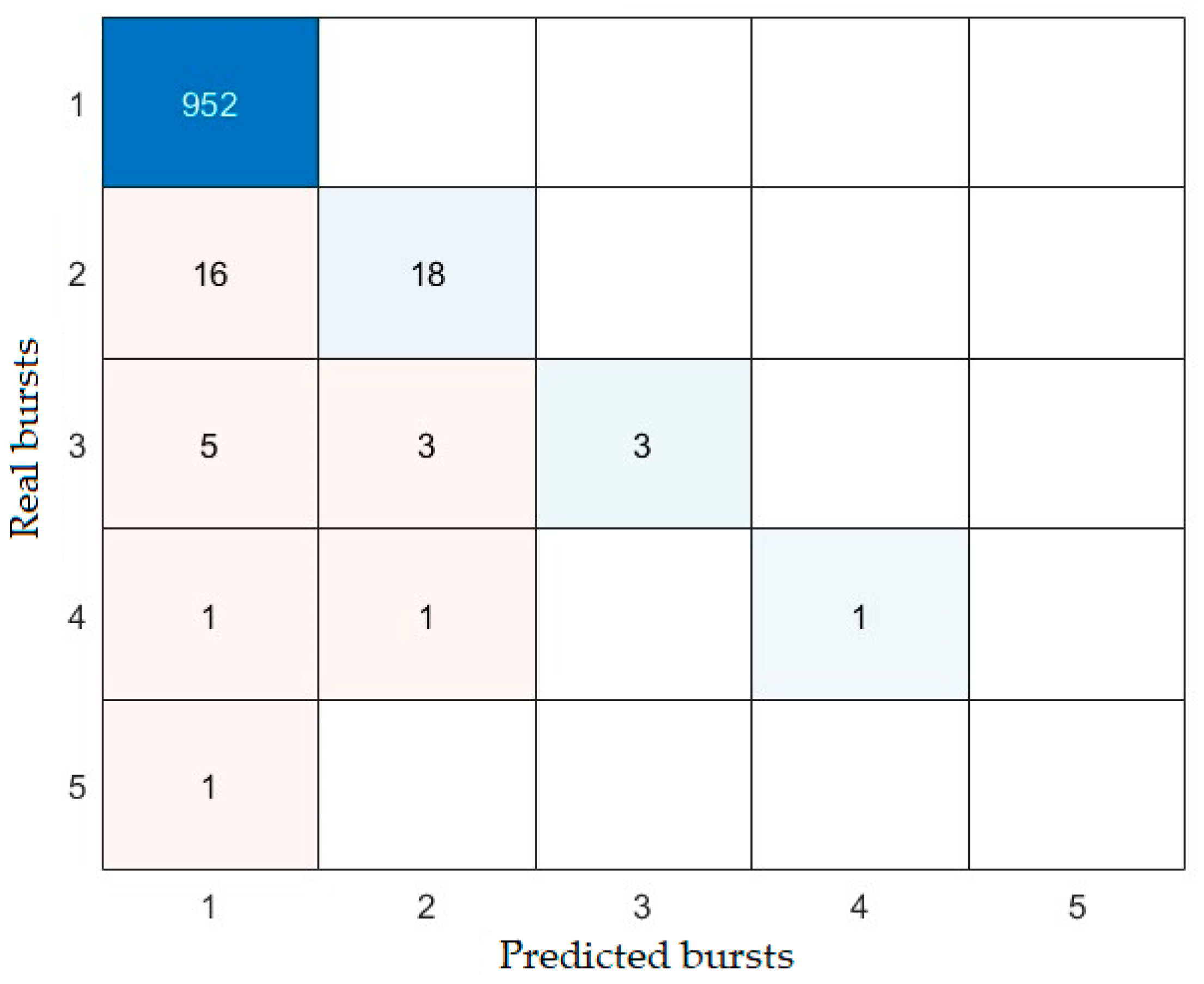
The classification of each pipe based on the number of bursts is evaluated by using a confusion matrix that allows for the visualization of the performance of the SVR algorithm by comparing the real number of failures with the estimated one. Figure 7 presents the confusion matrix, where each row of the matrix represents the number of real bursts, while each column represents the number of bursts predicted by the algorithm. The diagonal entries of the confusion matrix (represented by the blue colour) indicate the number of pipes where the algorithm accurately predicted the real number of bursts. For instance, the SVR algorithm correctly predicted that 952 pipes had one burst during the observation period. On the contrary, the off-diagonal values represent cases where the algorithm misjudged the real number of bursts. For example, the algorithm erroneously predicted that 16 pipes had one burst when, in reality, there were two bursts. It is important to highlight that, despite these discrepancies, the algorithm successfully predicted the majority of burst occurrences.

The determination coefficient is calculated, with values of 0.94 and 0.64, respectively, for the training and validation data. The determination coefficient results indicate a better performance for the SVR algorithm compared to linear regression.

Table 10. Pipe condition results using the SVR algorithm.

Condition Grade	SVR Algorithm
	Number of Pipes	Relative Frequency (%)
Good	687	41.24%
Average	976	58.58%
Unsatisfactory	6	0.18%
Total	1666	100%

presents the distribution of the physical pipe condition into three ranking levels defined according to the condition scale presented in Figure 1b for the SVR algorithm.

5. Discussion

Results have shown that the linear regression algorithm tends to overestimate the pipe condition rating, classifying pipes with worse conditions than the heuristic and SVR algorithms. The application of the three algorithms to the described case study resulted in different overall classifications for the same pipe. While the heuristic algorithm classified 60% of the pipes as average condition and 18% as unsatisfactory condition (considering answer-based weight and the entire survey group), the linear regression algorithm evaluated approximately 60% of the pipes as unsatisfactory condition (considering the linear model with the independent variables of average pipe age when the burst occurred and static pressure). Finally, the SVR algorithm classified approximately 60% of the pipes as average condition and almost all the remaining pipes as good condition.

The assessment of the physical condition of water distribution pipes combining the well-known performance indicator of the ratio of useful life (RUL) and the results of the three developed algorithms is presented in Figure 8. Results have demonstrated the following: the ratio of useful life tends to distribute pipe classification more equally in the three classes; the heuristic algorithm classifies most pipes as average condition; and the linear regression algorithm classifies most pipes as unsatisfactory condition. The SVR algorithm stands out as the main classifier for identifying pipes in good condition when compared to other algorithms. Additionally, it indicates that most pipes are classified in average condition and it only assigns three pipes to the unsatisfactory condition category.

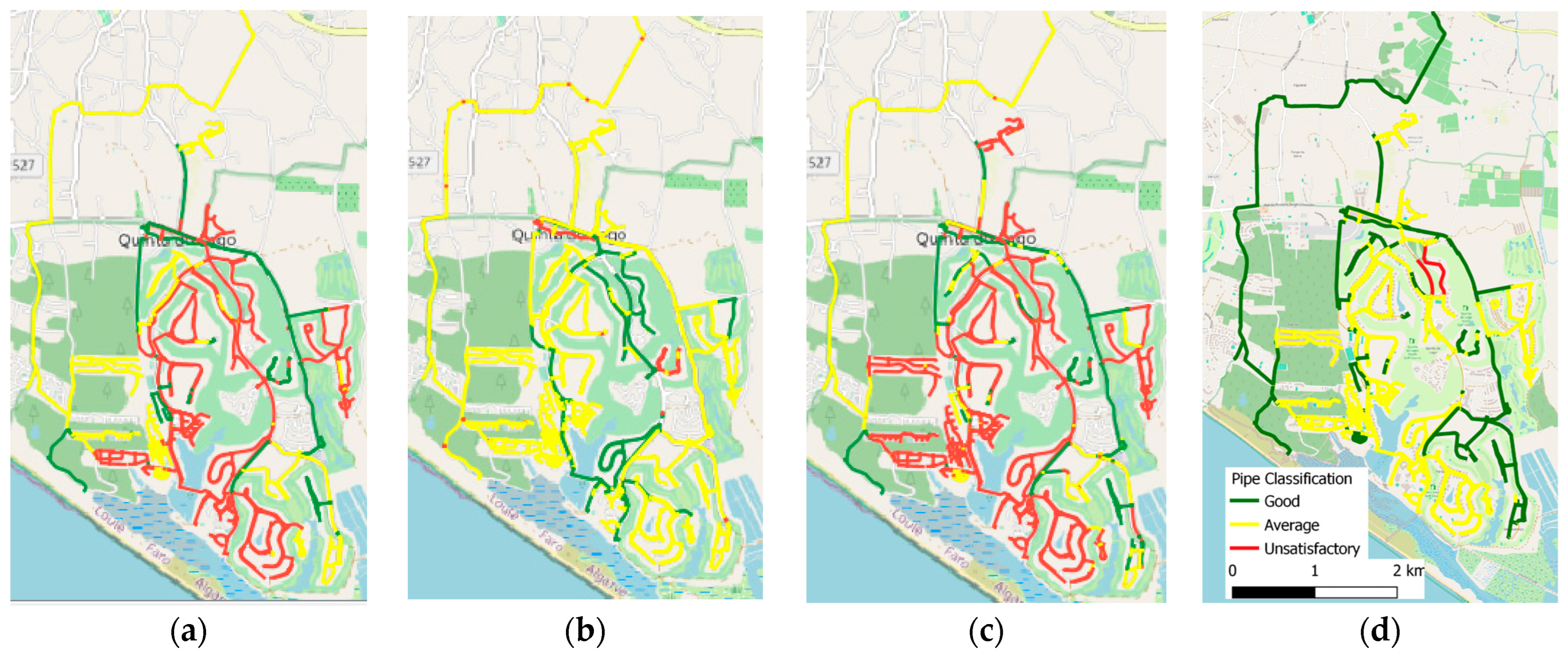
Figure 9 depicts the condition assessment maps obtained by the abovementioned three algorithms and the RUL. The pipes classified in unsatisfactory conditions by the ratio of useful life and the linear regression algorithm are almost the same, though the SVR algorithm is less conservative with a higher number of pipes in good and average condition.

Although different results were obtained, the development of a rehabilitation plan for a water distribution network should ideally integrate the results of these three algorithms to priority assets for intervention, i.e., the pipes classified as unsatisfactory and average condition in all algorithms. The cross-referencing of these three algorithms is described in

Table 11. Cross-referencing of three algorithms.

Same Condition Grade in the Three Algorithms	Number of Pipes	Relative Frequency (%)
Good	155	67%
Average	77	33%
Unsatisfactory	0	0%
Total	232	100%

.

The use of different algorithms for pipe condition assessment within water distribution systems has significantly improved the existing methods (i.e., RUL), since these allow for the inclusion of several factors that affect pipe deterioration as well as the use of advanced statistical tools and machine learning algorithms. The studied algorithms should be incorporated in the infrastructure asset management of urban water assets contributing to more informed and robust decision-making processes.

6. Conclusions

The prioritization of water distribution pipes for rehabilitation requires the assessment of the physical condition of assets. A methodology is proposed, including the following steps: data collection and validation, algorithm development and condition assessment. Three algorithms were studied and compared: the heuristic, linear regression and support vector regression algorithms. The proposed methodology allows for the assessment of the physical condition of assets without the need for extensive fieldwork or specific computational know-how, since it is based on the knowledge of simple infrastructure and operational data (e.g., pipe characteristics and operating conditions).

The application of the proposed methodology allowed for the assessment of the physical condition of a water distribution network located in Portugal. The results obtained from each algorithm were compared with a well-known performance indicator, the ratio of useful life. The results presented significant differences in their overall pipe condition classification. The linear regression algorithm allowed us to develop multiple linear regression models, considering different variables, such as the average pipe age when the burst occurred, the static pressure, the pipe material, the pipe length, the installation year and the distance to the tank. These models use the pipes with bursts during the period of observation as a training dataset. Consequently, the developed models include the notion that the structural condition of all other pipes will resemble the pipes that are presumably in worse condition (i.e., pipes that exhibited bursts during the period of observation). Therefore, this algorithm is considered to be highly penalizing in the classification of network pipes, classifying almost 60% of the network with an unsatisfactory condition.

On the other hand, the results from the heuristic and SVR algorithms were much less conservative, classifying the pipes as predominantly in average and good condition. In the heuristic algorithm, the following factors were considered: pipe material, pipe age, pipe nominal diameter, pipe length, pipe roughness coefficient and average operating pressure, pipe age being the most relevant factor in pipe deterioration. Different quantitative weights for each influencing factor were used; however, their order of influence does not change with the weights. In the SVR algorithm, different variables were used, such as the average pipe age when the burst occurred, the static pressure, the pipe material, the pipe length and the nominal diameter. The determination coefficients for the training and validation data were 0.94 and 0.64, respectively. These results indicate better performance from the SVR algorithm compared to linear regression.

Nevertheless, these three algorithms can be considered an improvement on the existing method of condition assessment through the use of the performance indicator ratio of useful life (RUL). This improvement is justified by the incorporation of several factors that influence pipe deterioration besides the asset age and its respective useful life. The application of the proposed methodology to a larger dataset with a higher period of observation should be carried out as future work. This would allow for the achievement of more robust results, as well as testing of the proposed methodology. Furthermore, the obtained results should be included in the decision-making process for pipe rehabilitation.

References

1. Naderi, M.J.; Pishvaee, M.S. Robust bi-objective macroscopic municipal water supply network redesign and rehabilitation. Water Resour. Manag. 2017, 31, 2689–2711. [Google Scholar] [CrossRef]
2. Carriço, N.; Covas, D.; Almeida, M.C.; Leitão, J.P.; Alegre, H. Prioritization of rehabilitation interventions for urban water assets using multiple criteria decision-aid methods. Water Sci. Technol. 2012, 66, 1007–1014. [Google Scholar] [CrossRef]
3. Alegre, H.; Coelho, S.T. Infrastructure Asset Management of Urban Water Systems. In Supply System Analysis—Selected Topics, 1st ed.; Ostfeld, A., Ed.; IntechOpen: London, UK, 2012; pp. 49–74. [Google Scholar]
4. Harvey, R.; de Lange, M.; McBean, E.; Trenouth, W.; Singh, A.; James, P. Asset condition assessment of municipal drinking water, wastewater and stormwater systems—Challenges and directions forward. Can. Water Resour. J. 2017, 42, 138–148. [Google Scholar] [CrossRef]
5. Alegre, H.; Covas, D. Infrastructure Asset Management in Urban Water Systems: An Approach Focuses on Rehabilitation, 1st ed.; ERSAR, LNEC, IST: Lisbon, Portugal, 2010; p. 510. (In Portuguese) [Google Scholar]
6. Urrea-Mallebrera, M.; Altarejos-García, L.; García-Bermejo, J.; Collado-López, B. Condition Assessment of Water Infrastructures: Application to Segura River Basin (Spain). Water 2019, 11, 1169. [Google Scholar] [CrossRef]
7. Liu, Z.; Kleiner, Y.; Rajani, B.; Wang, L.; Condit, W. Condition Assessment Technologies for Water Transmission and Distribution Systems; United States Environmental Protection Agency (EPA): Washington, DC, USA, 2012; p. 108.
8. Liu, Z.; Kleiner, Y. State of the art review of inspection technologies for condition assessment of water pipes. Meas. J. Int. Meas. Confed. 2012, 46, 1–15. [Google Scholar] [CrossRef]
9. Al-Barqawi, H.; Zayed, T. Condition rating model for underground infrastructure sustainable water mains. J. Perform. Constr. Facil. 2006, 20, 126–135. [Google Scholar] [CrossRef]
10. Selvakumar, A.; Morisson, R.; Sangster, T.; Boyed Downey, D.; Matthews, J. State of Technology for Rehabilitation of Water Distribution Systems; United States Environmental Protection Agency (EPA): Washington, DC, USA, 2013; p. 3.
11. Ugarelli, R.; Bruaset, S. Review of deterioration modelling approaches for ageing infrastructure. SINTEF Rep. 2013, 53, 1689–1699. [Google Scholar]
12. Al-Barqawi, H.; Zayed, T. Assessment model of water main conditions. Proceedings of Pipelines: Service to the Owner, Chicago, IL, USA, 30 July–2 August 2006. [Google Scholar]
13. Rajani, B.; Kleiner, Y. Comprehensive review of structural deterioration of water mains: Physically based models. Urban Water J. 2001, 3, 151–164. [Google Scholar] [CrossRef]
14. Alegre, H. Infrastructure Asset Management of Water Supply and Sewer and Treatment of Wastewater; LNEC: Lisbon, Portugal, 2008. (In Portuguese) [Google Scholar]
15. Rajani, B.; Makar, J. A methodology to estimate remaining service life of grey cast iron water mains. Can. J. Civ. Eng. 2000, 27, 1259–1272. [Google Scholar] [CrossRef]
16. Cassiolato, G.; Carvalho, E.P.; Caballero, J.A.; Ravagnani, M.A. Optimization of water distribution networks using a deterministic approach. Eng. Optim. 2021, 53, 107–124. [Google Scholar] [CrossRef]
17. St. Clair, A.M.; Sinha, S. State-of-the-technology review on water pipe condition, deterioration and failure rate prediction models! Urban Water J. 2012, 9, 85–112. [Google Scholar] [CrossRef]
18. Zhou, Y.; Vairavamoorthy, K.; Grimshaw, F. Development of a fuzzy based pipe condition assessment model using PROMETHEE. In Proceedings of the World Environmental and Water Resources Congress, Kansas, MO, USA, 17–21 May 2009. [Google Scholar]
19. Assad, A.; Bouferguene, A. Data mining algorithms for water main condition prediction—Comparative analysis. J. Water Resour. Plan. Manag. 2022, 148, 04021101. [Google Scholar] [CrossRef]
20. Alves Coelho, J.; Glória, A.; Sebastião, P. Precise water leak detection using machine learning and real-time sensor data. IoT 2020, 1, 474–493. [Google Scholar] [CrossRef]
21. Costa, A.; Cardoso, J.; Rosa, J.; Rodrigues, R.; Faroleiro, P.; Ruivo, F.; Videira, C.; Rosa, D.; Monte, M.; Santos, C.; et al. Annual Report on Water and Waste Services in Portugal (2020) Volume 1—Characterisation of the Water and Waste Sector; ERSAR: Lisbon, Portugal, 2020. [Google Scholar]
22. King, A.P.; Eckersley, R.J. Descriptive Statistics II: Bivariate and Multivariate Statistics. In Statistics for Biomedical Engineers and Scientists, 1st ed.; Mara Conner: London, UK, 2019; pp. 23–56. [Google Scholar]
23. Lambrinos, J. Applied Linear Regression Models. Technometrics 1984, 26, 415–416. [Google Scholar] [CrossRef]
24. Cawley, G.C.; Talbot, N.L.C. On Over-fitting in Model Selection and Subsequent Selection Bias in Performance Evaluation. J. Mach. Learn. Res. 2010, 11, 2079–2107. [Google Scholar]
25. Myers, R.H.; Montgomery, D.C.; Anderson-Cook, C.M. Response Surface Methodology: Process and Product Optimization Using Designed Experiments, 4th ed.; John Wiley & Sons: Hoboken, NJ, USA, 2016; p. 837. [Google Scholar]
26. Vapnik, V. The Nature of Statistical Learning Theory, 2nd ed.; Springer: New York, NY, USA, 2013; p. 313. [Google Scholar]
27. Alegre, H.; Matos, R.; Beja Neves, E.; Cardoso, A.; Duarte, P. Guide to Assess the Quality of Water and Waste Services Provided to Users, 3rd ed.; ERSAR: Lisbon, Portugal, 2021. [Google Scholar]
Figure 1. Condition assessment matrices with three ranking levels (good condition represented by the green colour, average condition represented by the yellow colour and unsatisfactory condition represented by the red colour): (a) heuristic algorithms; (b) linear regression and support vector regression algorithms.
Water 16 01318 g001
Figure 2. Water distribution network characteristics: (a) construction materials; (b) nominal diameter; and (c) construction year.
Water 16 01318 g002
Figure 3. Distribution of the duration of the professional career of surveyed experts.
Water 16 01318 g003
Figure 4. Obtained weight values for each influencing factor considering different weight formulations: (a) answer-based weights; (b) number of replies and answer-based weights; (c) median-based weights; (d) number of replies and median-based weights; (e) mean-based weights; and (f) number of replies and mean-based weights.
Water 16 01318 g004
Figure 5. Pipe material distribution: (a) good condition; (b) average condition; and (c) unsatisfactory condition.
Water 16 01318 g005
Figure 6. Pipe age distribution: (a) good condition; (b) average condition; and (c) unsatisfactory condition.
Water 16 01318 g006
Figure 7. Confusion matrix for the SVR algorithm.
Water 16 01318 g007
Figure 8. Distribution of pipe physical condition for the ratio of useful life and heuristic, linear regression and SVR algorithms.
Water 16 01318 g008
Figure 9. Color map for: (a) ratio of useful life; (b) heuristic algorithm; (c) linear regression algorithm; and (d) SVR algorithm.
Water 16 01318 g009