Article

Effect of Teleconnection Patterns on the Formation of Potential Ecological Flow Variables in Lowland Rivers

by
Karolina Gurjazkaitė
,
Vytautas Akstinas
* and
Diana Meilutytė-Lukauskienė
Laboratory of Hydrology, Lithuanian Energy Institute, 44403 Kaunas, Lithuania
*
Author to whom correspondence should be addressed.
Water 2024, 16(1), 66; https://doi.org/10.3390/w16010066
Submission received: 8 November 2023 / Revised: 15 December 2023 / Accepted: 21 December 2023 / Published: 23 December 2023
(This article belongs to the Section Hydrology)

Abstract

:
Climate is probably the most important factor affecting river discharge and flow dynamics. Low flows in rivers during the warm period cause stress to aquatic ecosystems and pose a challenge to sustainable water management. Previous research has shown that the average minimum discharge of the 30 driest continuous days, known as Q30, is a suitable measure for ecological flow estimation in Lithuania. This study aims to examine whether large-scale atmospheric processes, so-called teleconnections, can have an impact on Q30 during the warm period. Hydrological data for 1961–2020 from 25 water gauging stations were used to search for hydrological response signals with five selected climate indices (NAO, SCA, POL, EA/WR, and EA). Pearson correlation and Wilcoxon–Mann–Whitney test approaches were applied. The results suggested that the EA/WR and NAO had the strongest influence on Q30 in the studied region during the warm period. The positive phases of the indices tended to cause a greater decrease in Q30 values due to the prevailing easterly edge of the anticyclonic circulation over the studied region determined by the EA/WR and NAO indices, while the negative phases of the mentioned indices caused an increase and greater dispersion of Q30.

1. Introduction

Climate is undeniably the most important factor that profoundly affects the hydrology of surface waters, from small streams to large rivers. It determines the intricate interaction of precipitation, temperature, and evaporation, influencing both the availability of water and the well-being of aquatic ecosystems. This transition from climate to rivers reveals a close link between climatic conditions and surface water hydrology [1,2,3]. The amount and timing of precipitation have a direct influence on river flows and dictate discharge and seasonal variations. At the same time, regional temperature dynamics influence thermal conditions, habitats, and aquatic life cycles. In combination with human-induced influences, this climatic control has a significant impact on water resources. For rivers, this means an unbalanced flow regime and increased flood and drought cycles, which make river management more difficult and overwhelm the demands of society [4,5].
Understanding the dynamics of river flows is crucial for sustainable river management. Both natural and anthropogenic factors influence river discharge. These factors include precipitation, temperature, vegetation cover, soil characteristics, and many more. This complex relationship between rivers and their environment has been thoroughly investigated in numerous studies. Some researchers have focused on the links between changes in river discharge and overall global changes in precipitation and temperature patterns [6,7], including regional analyses in Europe [4,8,9]. Other studies deal with the influence of anthropogenic factors on river discharge. For example, hydrological changes in the flow regime of rivers, which benefit human development in many ways, have an impact on the provision of ecosystem services. Studies in this regard provide a wealth of evidence on the negative impacts of economic activities on European rivers [10,11,12,13]. Effective river management requires a comprehensive understanding of the complex interplay of these factors to ensure the responsible allocation of water resources. Understanding the causality of changes in river discharge is extremely important as it allows us to unravel the complex network of factors that influence river discharge [14,15,16]. These factors, which have a profound influence on river discharge, include a wide range of natural and anthropogenic elements [17,18].
Atmospheric circulation patterns play an important role in the formation of runoff and can be a primary source of generative forcing for river systems. Extensive research around the world, including studies in Europe, has demonstrated the influence of different large-scale atmospheric circulation patterns on the climatic characteristics and hydrological behaviour of rivers and lakes [19,20,21,22,23,24,25]. For example, the seasonal variations in dryness and wetness and their links with large-scale atmospheric circulation and global sea surface temperature have been analysed [26]. Particularly noteworthy is the dynamic nature of these relationships, which vary and differ from one season to the next. Plewa et al. [23] focused on the links between lake water levels and indices of macroscale atmospheric circulation. An analysis of the relationship between water temperature and large-scale atmospheric circulation was also carried out [21]. Pandžić et al. [27] analysed the relationships between large-scale atmospheric circulation and monthly precipitation and river discharge. Some studies have assessed the impact of teleconnections on runoff [28,29,30]. The results of Lorenzo-Lacruz et al. [30] showed the dynamic interplay between runoff and atmospheric circulation in recent decades. Furthermore, the relationships between atmospheric circulation patterns and water surface temperature along the coast of the southern Baltic Sea were also investigated [31].
The coupling analysis of variations In runoff with Iic teleconnection Indices showed significant correlations between runoff and the selected teleconnection indices [29]. This correlation highlights the important role that these indices play in runoff and its dynamics. In Europe, some studies have shown that river discharge is influenced by teleconnection patterns such as the North Atlantic Oscillation (NAO) and the Arctic Oscillation (AO), depending on the region and season [26,32,33]. The NAO has also been used as a model input for the prediction of winter runoff in large rivers in Europe [34]. For Northern Europe and the North Atlantic region, Kingston et al. [35] conducted a comprehensive study on the complicated interplay between large-scale atmospheric circulation and runoff. Their study revealed a complex relationship and made it clear that the link between Northern Hemisphere circulation indices and regional climate variables depends on the specific time scale and time periods considered in teleconnection studies. In addition, Bouwer et al. [36] provided valuable insights by showing significant correlations between the frequency of the western circulation type of large-scale weather conditions and discharge in different river catchments of Northern and Western Europe. Regional sensitivities of mean and maximum river discharge to climate variability using up to 608 stations across Europe have shown that the annual maximum discharge is more sensitive to atmospheric circulation variability than mean discharge [37]. Mean discharge fluctuated on average between 8 and 44%, while the peak discharges varied between 10 and 54% per index unit, with the discharges in Iberia and Scandinavia being more sensitive than those in Central and Western Europe. Studies in the central–eastern parts of Europe have shown contrasting results. The studies on discharge anomalies showed a weak correlation with the NAO, East Atlantic (EA), and Scandinavian (SCA) indices, while the East Atlantic/Western Russia (EA/WR) pattern had a stronger influence on discharge, especially in winter [27]. In the Mediterranean region, an analysis of possible links between the NAO and runoff revealed that topographic effects weaken the impact of the NAO on runoff reduction [38]. In the United Kingdom, an analysis of the River Ewe showed that the NAO and the AO have an impact on different runoff characteristics, especially in winter months [39]. In Central Finland, the analysis and variability of dryness and wetness and the role of teleconnection patterns were estimated [40]. The impacts of these teleconnections were best distinguished on annual, seasonal (all seasons except winter), and monthly time scales (in warm months). In addition, the NAO correlated positively with dryness and wetness, especially in the winter and cold months; the NAO was also the strongest atmospheric driver of all teleconnections in the study. In Sweden, the spatio-temporal effect of atmospheric teleconnection patterns on river discharge showed that river discharge during the accumulation period had a negative correlation of −0.44 with the SCA index averaged over the same period [41]. At the same time, there was a positive correlation of 0.42 with the NAO and 0.59 with the AO, in each case with a lead time of zero months and a 2-month time window. This means that the interaction between these teleconnection patterns can lead to either a positive or negative influence on their activity, which in turn leads to an increase or decrease in their individual impact on runoff in a linear or non-linear manner. In the western and southern parts of Romania, Birsan [28] found a strong negative correlation between the NAO and mean annual runoff. This correlation underlines the significant influence of the large-scale atmospheric circulation on the annual runoff discharge in these areas, as well as the important orographic role of the Carpathian Mountains. Stahl and Demuth [42] conducted a very detailed study of 74 basins in Germany and found that the effects of atmospheric circulation patterns and the response of runoff can be regionalised. The results showed considerable regional differences in the time lag of the response to drought and the corresponding atmospheric circulation patterns.
All previously mentioned studies have highlighted the role of atmospheric circulation in hydrological processes. For the selected region (in Lithuania), the low flow period in the rivers and its dependence on many factors is also a very important issue. Šarauskienė et al. [43] found that the intermittency of rivers in the surplus water zone is also related to atmospheric circulation and that intermittency processes are associated with the SCA index. Nazarenko et al. [44] claimed that the effects of climate change are noticeable in discharges in the western and central parts of Lithuania during low flow periods. The application of the HBV model has shown that climate change will affect low flow indicators, including the multiannual minimum and average of low flow, and that the impact will vary depending on the feeding source of the rivers [45]. The importance of low flow parameters was drawn by Virbickas et al. [46], as these indicators can be used to estimate warm season ecological flow (e-flow). The mentioned study conducted a hydro-ecological assessment based on the MesoHABSIM habitat modelling approach and determined the e-flow criteria by assessing the habitat needs of four cyprinid species found in regulated rivers. The e-flow suitable to fulfil the habitat needs of these species and indicative of good ecological status is represented by the multiannual mean of the average minimum discharge of 30 continuous days during the warm season (May–October). Moreover, the low flow and e-flow are linked in that ecological considerations should also be made during low flow and ensure that rivers maintain their ecological and environmental functions, even when the flow is reduced [47,48]. Short-term stressful low flows in Lithuania typically occur in late summer or early autumn [44]. All these findings call into question the current ecological flow regulation, which requires water users (primarily hydropower plant operators) to maintain a water flow equal to the multiannual mean of the average minimum discharge of 30 continuous days (Q30).
A review of various studies revealed the complex interplay between teleconnection patterns and various hydroclimatic variables. While there are few studies specifically linking teleconnections to low flow, it can be used as one of the potential variables for ecological flow estimation. This highlights the need for region-specific studies to understand the complex relationships between the atmospheric circulation indices and runoff characteristics of target rivers. Moreover, there is a general lack of assessment of influence of large-scale atmospheric circulation processes on various discharge indicators in the studied region and neighbouring regions. Previous studies conducted in other regions of Europe indicate that the effect of teleconnections can be regionalised, making it necessary to investigate these processes at smaller scales. Therefore, in this study, we have attempted to assess in detail the impact of teleconnection patterns on Q30 at a country level. The aim of this study is therefore to evaluate the effects of atmospheric circulation indices on lowland rivers in the south-eastern part of the Baltic Sea region. The focus was on Lithuanian rivers and their low flow variable Q30, which could be used to estimate the potential ecological flow during the warm season. Five teleconnection patterns expressed by circulation indices, North Atlantic Oscillation (NAO); Scandinavian pattern (SCA); Polar/Eurasian pattern (POL); East Atlantic/Western Russian pattern (EA/WR); and East Atlantic pattern (EA) [49], were used in this study. The main tasks in order to achieve the study objectives were to: (i) estimate the linear relations between the climate indices and Q30; (ii) assess the relation between the climate indices and Q30 using a non-parametric method and different temporal delay scenarios; (iii) evaluate the relationship between the climate indices and precipitation as drivers for low flow formation; and (iv) indicate the predominant atmospheric circulation over the study region during the low flow events. A better understanding of these drivers and their patterns can lead to more effective and sustainable water resources management, as well as prediction and preparedness for extreme events and hazards.

2. Study Area and Data

The focus of this study is on Lithuanian rivers. Lithuania is located in the south-eastern part of the Baltic Sea region. The country covers an area of 65.3 thousand km2 and is characterised by a dense river system, consisting of over 22,000 local and transboundary rivers and streams. The geographical and climatic conditions of Lithuanian rivers are similar to those of other rivers in the eastern and southern parts of the Baltic Sea basin region. Therefore, the findings of this study can be applicable to other countries in the Baltic Sea region when it comes to understanding the natural mechanisms that determine the behaviour of rivers. All rivers in the country can be categorised as lowland rivers due to the low altitude of their catchment areas (less than 300 m above sea level) [50]. Based on the Köppen–Geiger climate classification system, the Lithuanian climate is defined as a humid continental climate, with an average annual temperature of 7.4 °C and an annual precipitation of 695 mm for the period 1991–2020 [51]. In the country, the analysed low flow periods typically occur from August to September, occasionally from June to October, and very rarely beyond this period. These extended periods are mostly influenced by low precipitation and high temperatures, which increase evaporation. Twenty-five water gauging stations (WGSs) were selected for this study and are distributed across the entire study area (Figure 1).
The selected WGSs provided very reliable discharge data for the period 1961–2020 (Table 1). These WGSs cover catchments with an area of 100 to 1000 km2 (7 WGSs), 1000 to 6000 km2 (13 WGSs), and over 10,000 km2 (5 WGSs). These data were obtained from the hydrological yearbooks of the Lithuanian Hydrometeorological Service under the Ministry of Environment. Only uninterrupted data series or those with only a few interruptions were used for this study (e.g., Šušvė–Josvainiai had 4 years of missing data, Dubysa–Lyduvėnai—2 years, Lėvuo–Kupiškis—6, and Bartuva–Skuodas—1).
Table 1. Main characteristics of the selected water gauging stations and order of dominant multiannual feeding source (g—groundwater, s—snow melting, r—rainfall; a capitalised letter indicates that the feeding source accounted for more than 50% of the total runoff).
No.RiverWGSCatchment Area (km2)Qannual of 1961–2020 (m3/s)qannual
(l/s × km2)
Q30 of 1961–2020 (m3/s)q30
(l/s × km2)
Feeding Source *
1.NemunasDruskininkai37,382.32025.41123.0G-sr
2.NemunasNemajūnai42,869.02475.71423.3G-sr
3.NemunasSmalininkai81,129.74936.12683.3G-sr
4.MerkysPuvočiai4296.931.67.421.85.1G-sr
5.ŪlaZervynos679.04.827.12.934.3G-sr
6.ŽeimenaPabradė2595.420.37.812.14.7G-sr
7.VerknėVerbyliškės694.35.007.22.163.1g-sr
8.StrėvaSemeliškės234.01.647.01.004.3G-sr
9.NerisVilnius15,218.898.76.561.64.0G-sr
10.NerisJonava24,544.91636.690.73.7G-sr
11.ŠventojiAnykščiai3572.026.57.410.32.9g-sr
12.ŠventojiUkmergė5381.138.97.214.52.7g-sr
13.ŠušvėŠiaulėnai162.41.177.20.1490.9r-sg
14.ŠušvėJosvainiai1078.65.505.10.6230.58r-sg
15.DubysaLyduvėnai1073.28.367.82.021.9r-sg
16.ŠešuvisSkirgailai1876.314.98.02.471.3R-sg
17.JūraTauragė1664.121.913.13.712.2R-sg
18.AkmenaPaakmenis314.04.2613.60.6922.2R-sg
19.MinijaKartena1220.116.513.52.922.4R-sg
20.BartuvaSkuodas616.77.5012.20.7551.2R-sg
21.VentaPapilė1560.09.666.21.661.1r-sg
22.VentaLeckava4060.029.57.35.241.3r-sg
23.NemunėlisTabokinė2744.119.47.13.081.1r-sg
24.MūšaUstukiai2284.410.24.51.370.60r-sg
25.LėvuoKupiškis303.31.735.70.1520.50r-sg
Note: * According to Akstinas et al. [52].
Monthly precipitation data from 12 meteorological stations (monitored by the Lithuanian Hydrometeorological Service) covering the main selected river catchments were used for the climate data. Finally, five teleconnection patterns were selected: the North Atlantic Oscillation (NAO), the Scandinavian (SCA), the Polar/Eurasian (POL), the East Atlantic/Western Russian (EA/WR), and the East Atlantic (EA). These indices were selected on the basis of their known influence on the regional climate in most parts of Europe. The monthly data of the standardised indices for the period from 1961 to 2020 were provided by the National Oceanic and Atmospheric Administration (NOAA), National Weather Service, and Climate Prediction Centre (https://www.cpc.ncep.noaa.gov/data/teledoc/telecontents.shtml, last accessed on 6 November 2023). The NCEP–NCAR Reanalysis 1 data for the maps of geopotential height anomalies were provided by the NOAA Physical Sciences Laboratory (https://psl.noaa.gov, last accessed on 6 November 2023).

3. Methods

The aim of the present study is to quantify possible relationships between large-scale atmospheric circulation processes (known as teleconnections) and low flow parameters expressed by Q30, i.e., the average minimum discharge of the 30 driest continuous days. For this purpose, the annual Q30 values of the warm season (May–October) were derived from daily hydrological observations for each WGS. Moreover, the date (month and day) on which the Q30 event occurred was recorded. Five atmospheric circulation indices (NAO, SCA, POL, EA/WR, and EA) and their monthly standardised values were considered to establish possible relationships between large-scale atmospheric circulation processes and Q30. To investigate possible accumulative delay effects of the atmospheric circulation processes, six different scenarios of temporal delay were developed. Scenarios 0, consisting of A, B, C, D, E, and F, differed in the duration of the specific atmospheric circulation index value tested with Q30. In scenario A, an effect was sought based on the previous month’s index value; in scenario B, the sum of the previous two months’ index values was considered; the monthly range was also extended in scenarios C (3 months), D (4 months), E (5 months), and F (6 months). This set of scenarios was supplemented by an additional adjusted scenario that took into account the day of the Q30 event, namely, Scenario 1 with attribution to accumulative months, i.e., A1, B1, C1, D1, E1, and F1. If Q30 was recorded on days 1 to 15 of the month, scenarios A1 to F1 behaved exactly like their counterparts A to F. However, if the Q30 event occurred on day 16 to the end of the month, scenario A1 tests Q30 against the index value of the same month. The other scenarios were constructed accordingly, i.e., the index value of the same month plus 1 previous month was used for scenario B1, 2 previous months for C1, 3 previous months for D1, 4 previous months for E1, and 5 previous months for F1.
Two quantitative approaches were used to determine the relationship between the indices and Q30. In the first approach, Pearson’s correlation coefficient was calculated between the annual series of atmospheric circulation index values and a corresponding series of Q30 values of all analysed years to check whether there was a linear relationship between the two datasets. In addition, the linear relationships between the monthly precipitation amount and the monthly standardised values of the individual climate indices were tested. The analysis was performed for six different accumulation periods (1 to 6 months), as in the case of Q30, to cover up to half a year of possible climate signals on precipitation patterns. The potential lag of precipitation with respect to the variability of the climate indices was tested up to 12 months before the precipitation month.
In the expectation of possible relationships, an alternative approach was considered, namely, the use of the Wilcoxon–Mann–Whitney test [53]. This test is a non-parametric method that can be used to quantify whether two populations are statistically identical under the null hypothesis or whether one population tends to have higher values than the other. It divides the dataset into two equal populations accordingly. The test was applied as follows: the first 20 and the last 20 years were selected from all years of a single time series (each corresponding to a particular combination of WGS, Q30 value, and accumulative delay scenario of the index) ordered by the atmospheric circulation index. Each of the resulting 40 years was assigned either a first rank (the first 20 years with a negative phase of the index) or a second rank (the last 20 years with a positive phase index). The second step of the ranking was ordered by Q30 (from lowest to highest), resulting in ranks 1 to 40. Finally, the two sets of ranks (negative and positive phases of the index) were compared using the Wilcoxon–Mann–Whitney test according to the ranking of the second step. The results of the test were categorised into statistical confidence levels of 90%, 95%, and 99%, but only results of ≥95% were considered statistically significant and interpreted as there being a high probability of an effect of the climate indices on Q30.
Based on the statistically significant relationships, the anomalies of the geopotential height of the isobaric 500 hPa surface (Z500) were calculated to indicate the main atmospheric circulation situations over the studied region. The anomaly maps were generated using the NOAA Physical Sciences Laboratory (PSL) Monthly Composites application (https://psl.noaa.gov/cgi-bin/data/composites/printpage.pl, last accessed on 6 November 2023). To create the maps, for each rank (first and second rank of each index), a set of 5 of the most frequent years with statistically significant relationships between the WGSs was selected from the top and bottom rankings according to Q30. Therefore, 5 of the 20 selected years (25%) were used to indicate the prevailing atmospheric circulation over the target region during the negative and positive index phase based on the Q30 size. The same years were used to create the heatmaps of the temporal change of the Z500 anomalies over the year to highlight the main development features between 40 and 60° N latitude and from 45 W to 45 E longitude during the low and high Q30 values.

4. Results

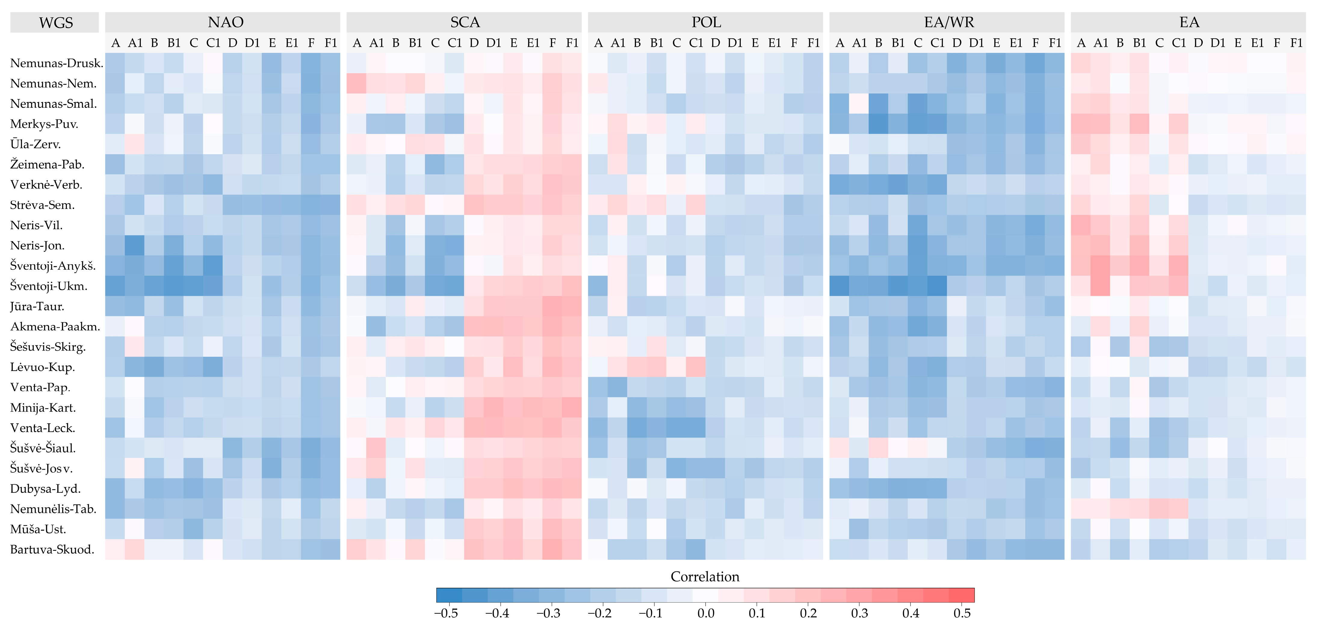
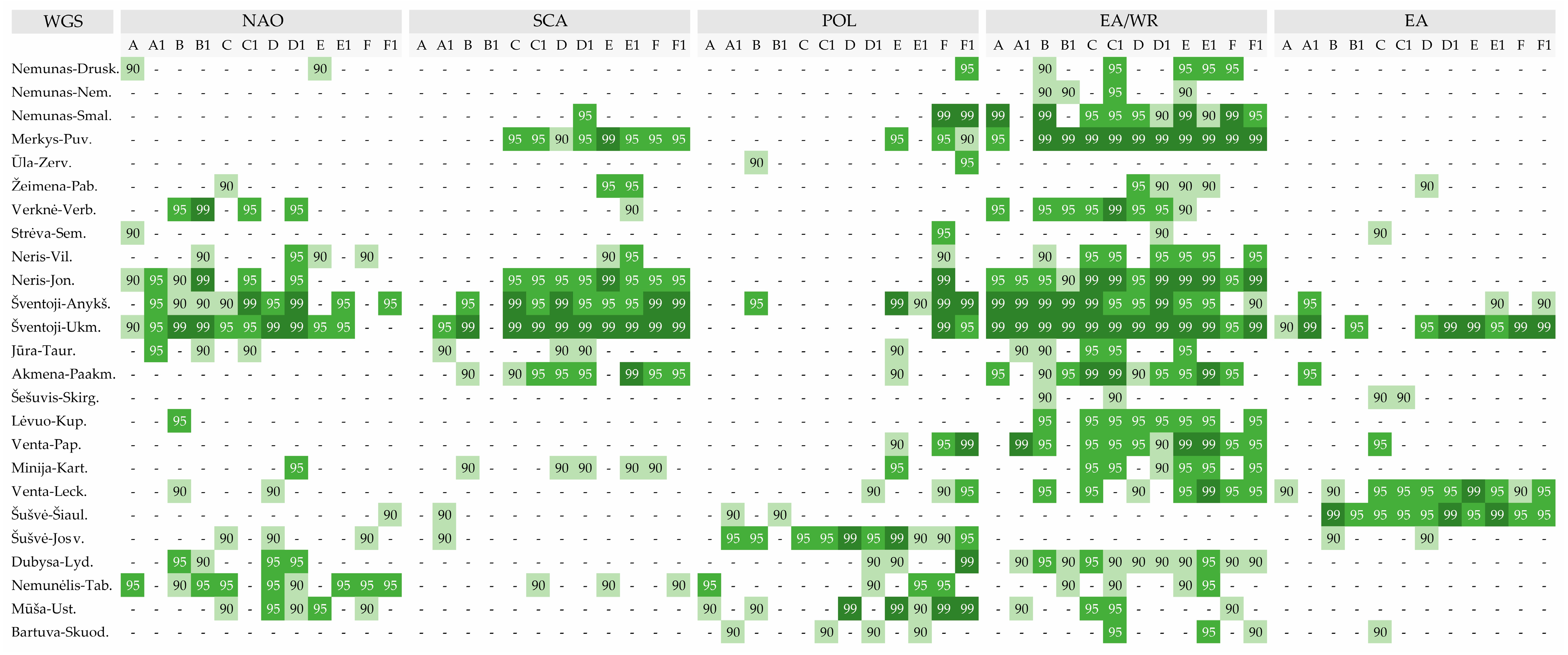
4.1. Correlation Analysis between Climate Indices and Low Flow

In the first phase of the data analysis, the Pearson correlation coefficient was calculated to investigate possible relationships between the data series of the annual Q30 values of each analysed WGS and the series of the corresponding indices at each temporal delay scenario. In most scenarios, there were negative correlations between Q30 and the indices (Figure 2). To maintain hydrological similarities, the order of the rivers based on hydrological regionalisation was applied [52]. Most correlations were relatively weak. On average, the correlation between the NAO index and Q30 was −0.187 but ranged from −0.43 to 0.13 and was mostly negative. The weakest correlations occurred in the A1 scenario with a 1-month temporal delay (−0.12 on average). However, as the accumulative lag increased, the negative correlations became more pronounced, dropping to −0.28 in scenario F (6-month lag). There were some groups of rivers that reacted similarly to the index. The Šventoji River, a tributary of the Neris, displayed relatively stronger correlations in the first six scenarios (A to C1, with a lag of 1 to 3 months). Additionally, the Neris River also showed more pronounced negative correlations with the Šventoji catchment area for scenarios A1, B1, and C1, which fell to −0.43.
The correlation between Q30 and the SCA index was relatively low on average (0.037), but correlation coefficients ranged from −0.38 to 0.26, depending on the scenario. The group of rivers consisting of the WGS of Neris and Šventoji had the relatively strongest correlation coefficients for scenarios B, C, and C1 and included an average coefficient of −0.34 for the mentioned scenarios. For the longer accumulative period of scenarios, D to F (4 to 6 months), the correlation gradually became positive. This regularity indicates the possible opposite effect of the longer accumulative lag time compared to the shorter one.
Correlations between the POL index and Q30 ranged from −0.36 to 0.2, but the overall tendencies indicated more cases of negative correlation. The relatively strongest negative correlations were found in the WGSs in the western part of Lithuania. Here, the strongest coefficients reached −0.36 according to scenarios B, C, and C1. The increased lag time of 4and 6 months decreased the correlation for most rivers.
The EA/WR index showed the most pronounced results, as the correlation coefficients varied from −0.46 to 0.12. Most correlations were negative. The response of Q30 to the EA/WR index gradually increased on average from −0.16 at 1-month lag (scenario A1) to −0.27 at 3-month lag (scenario C). The relationship between EA/WR and Q30 in scenarios D and E decreased but remained as strong as in scenarios F and F1. The average correlation per scenario was −0.25 for F and −0.27 for F1. Šventoji-Anykščiai WGS showed the relatively highest values for 2- and 3-month lags (all scenarios B and C, with correlations averaging −0.42 across these scenarios). Further relatively stronger correlations occurred in scenarios B, C, and C1 at Verknė–Verbyliškės (−0.36), Merkys–Puvočiai (−0.35), Dubysa–Lyduvėnai (−0.30), and Nemunas–Smalininkai (−0.36) WGSs.
The relationships between Q30 and the EA index indicated the relatively weakest correlations despite the large variability from−0.28 to 0.30 but, on average, the correlations for each given scenario were low (0.09 to 0.07). The rivers in eastern Lithuania (Nemunas and its tributaries) show slightly positive correlations in scenarios A to C (1- to 3-month lag). Most of the values in scenarios D to F1 were close to zero.

4.2. Climate Indices’ Signals in Low Flow Data

The Wilcoxon–Mann–Whitney test was performed to determine dependencies between the analysed atmospheric circulation indices and Q30 at the same 25 water gauging stations. The relations between the climate indices and the low flow parameter were tested for different scenarios of temporal response from the onset of the oscillation to the Q30 event, corresponding to the same scenarios from A to F1 with accumulative lag times from 1 to 6 months. The results showed whether the climate index signal on Q30 of certain WGS was reflected according to the different delay scenarios and what the statistical significance of the relationship found (Figure 3).
The EA/WR climate index had the strongest relation with the Q30 of the studied rivers. In most WGSs (20 out of 25), the statistically significant relations (with a confidence level of ≥95%) were found at least once per analysed scenario (Figure 3). For other climate indices such as the NAO and SCA, statistically significant relations were only found for 11 and 8 WGS, respectively, in 16 analysed scenarios. For the NAO index, the strongest response occurred in scenarios with an accumulative lag of 4 months (scenarios D and D1; 7 and 5 WGS, respectively, showed a statistically significant relationship). The weakest response was seen in scenarios A, E, E1, F, and F1, with only 1–3 WGS in each of these scenarios showing a significant relationship with the NAO. Q30 of the Neris River and its tributary Šventoji River were strongly influenced by the NAO and the peak strongest response was observed in scenarios C1, D, and D1, implying a lag of 3–4 months. Two WGSs, Mūša–Ustukiai and Nemunėlis–Tabokinė of northern Lithuania, also displayed significant responses to the NAO according to different scenarios (Figure 3).
To illustrate the character of the relations, the distribution of the standardised values of Q30 assigned to the first rank (negative index phase) and the second rank (negative index phase) was also presented on the basis of the statistically significant relations (Figure 4). The 20 years with the highest (positive) NAO values corresponded predominantly to one third of the lowest Q30 values. In contrast, the 20 years with the lowest (negative) NAO values did not correspond to any specific Q30 value but showed a tendency for Q30 values to increase during the negative phase for most scenarios.
For the SCA index, the relationship between the index and Q30 occurred at several stations in scenarios C to F (3- to 6-month lag), with the peak response occurring in scenarios D and E with 4- and 5-month lags, respectively (Figure 3). The highest number of statistically significant relationships was found in the Neris and Šventoji group of rivers, with no obvious peak, and in Merkys, where the peak in scenario E corresponded to a 5-month accumulative delay. Akmena–Paakmenys also responded strongly to this index, with the highest values occurring in scenario E1, which corresponds to a 5-month accumulated delay. This type of relationship occurs most frequently in scenario E1, suggesting that Q30 responds to the oscillation with a 4-month accumulative delay. The 20 years with the highest (positive) SCA values accumulated in the lower half of the Q30 values, and similarly to the NAO, the 20 years with the lowest (negative) SCA values were spread over a wide range of Q30 values but tended to increase Q30 (Figure 4). Sixteen WGS had a statistically significant relationship with POL, and the most significant relationships occurred in the scenarios with the longest cumulative delays F and F1, corresponding to 6 months (Figure 3). This index seems to have much weaker effects in the other scenarios, with the exception of Šušvė–Josvainiai, which had continuously shown significant responses to the changes in this index. The obtained signalling character tended to decrease the Q30 values with the increase of the POL index within the positive phase, as the 20 highest values of the positive oscillation corresponded to the lower half of the Q30 values, while the 20 lowest values of the POL index were associated with an increase of Q30 (Figure 4).
The EA/WR index interacted most strongly with the potential ecological flow variable of Q30 compared to the other climate indices, regardless of the time lag. However, this index showed the strongest impact on Q30 at an accumulated delay of 3 months before the Q30 event, as scenarios C and C1 had 15 and 16 WGS, respectively, with a statistical confidence level of ≥95% (Figure 3). A second and smaller peak of the WGSs involved occurred 5 months before the Q30 event. The effect of the index is visible on most of the analysed rivers, but the largest response to the EA/WR index was shown for the Neris and Šventoji River group. Similarly, to other scenarios, Q30 tends to be low during the positive phase of the index, while negative index values were accompanied by multiple high Q30 values (Figure 4). In contrast to EA/WR, EA seemed to have the weakest impact on the studied area during the dry period, where only six WGSs responded statistically significantly to this index (Figure 3). Only Venta–Leckava and Šušvė–Šiaulėnai had some repeated statistically significant tendencies within the different scenarios, with no clearly defined accumulation time when this index would have the strongest impact on Q30.

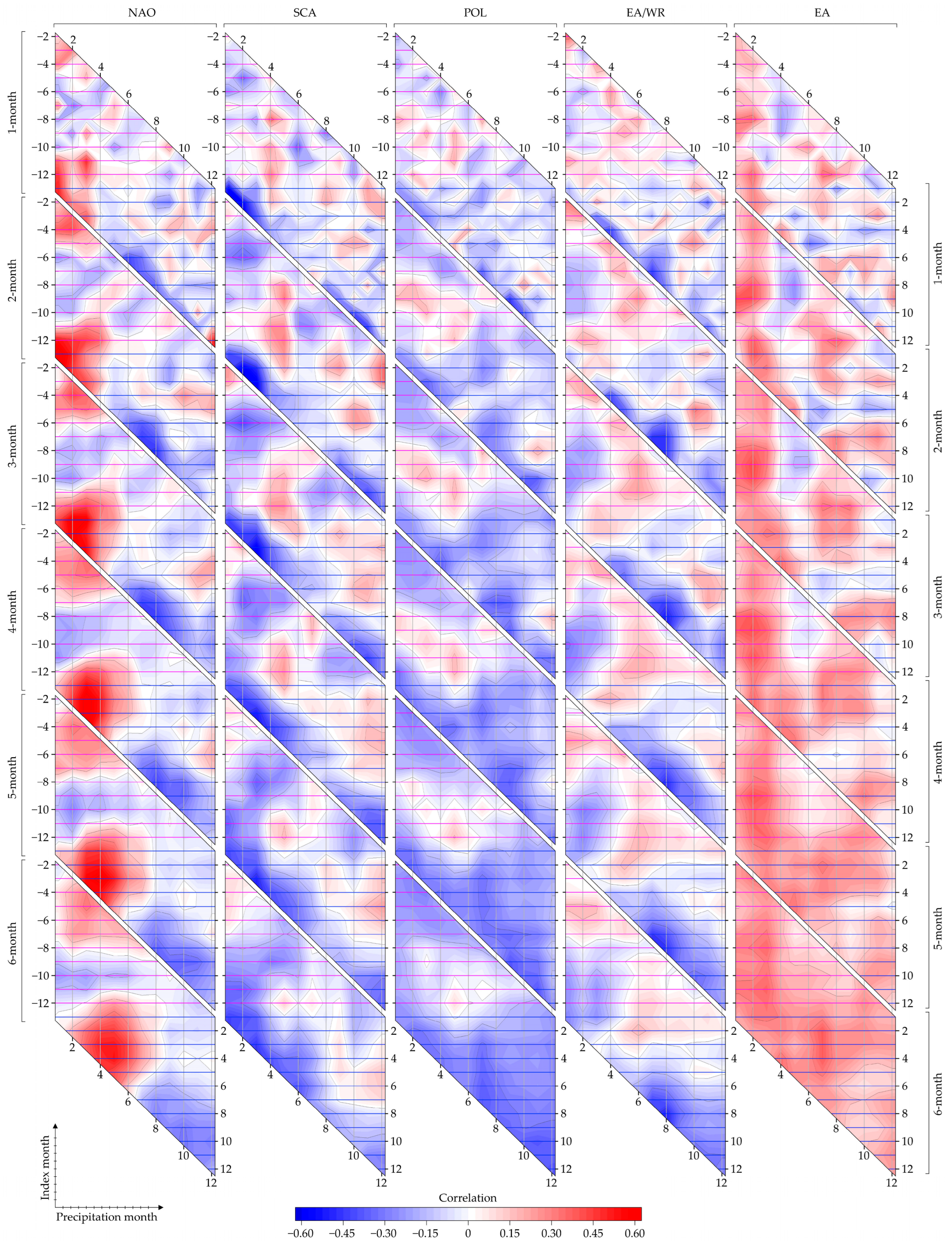
4.3. Climate Indices Relation with Precipitation

Based on the previous results, the relations between monthly precipitation and the monthly average of each climate index were tested. This analysis was used to reveal whether a linear relation exists between the climate indices and the amount of precipitation over Lithuania, as precipitation plays an important role in the formation of low flows and river flow in general. The relations were analysed for six different cumulation periods ranging from 1 to 6 months (Figure 5). The results also indicated the potential lag of precipitation with respect to the climate signal, as the relations were tested up to 12 months before the precipitation month. The relatively strongest correlations were found for the NAO and EA/WR indices. For the 1-month accumulation period, the strongest relationships with the warm season were defined in June for the NAO index, in July for the EA/WR index, and in September for the POL index. All these indices were negatively correlated with precipitation and their coefficients varied between −0.42 and −0.45. Only the correlation between the SCA index and precipitation reached −0.50, but the strongest relations were found in the cold months of January, February, and November. Meanwhile, the NAO index correlated positively with precipitation and had a correlation coefficient of 0.50 at the beginning of the year. Longer accumulation periods increased the correlations between precipitation and the NAO, SCA, and EA/WR climate indices. The relatively highest correlation between the NAO and precipitation was found for a 4-month accumulation period, but the strength of the relationship depended on the season. In the cold season, the relatively highest positive correlation (0.64) was found in March, while in the warm season, the negative correlation of −0.43 was found in August. The strongest relationship between the EA/WR index and precipitation was found for the 3-month accumulation period, as the correlation was 0.51 in August. The extended accumulation period up to 5 and 6 months strengthened the relations for the POL index but did not noticeably change the correlation for the EA/WR index. The relatively weakest relations were obtained for the EA index and despite the accumulation period, the correlation coefficients did not exceed 0.30 in the warm season. All these results indicate the existing linear relations between some of the climate indices and precipitation, which could explain the influence of the indices on the low flow parameters. Therefore, the following analysis of the differences in the atmospheric circulation expressed by the geopotential height anomalies was performed to explain the potential influencing mechanisms.

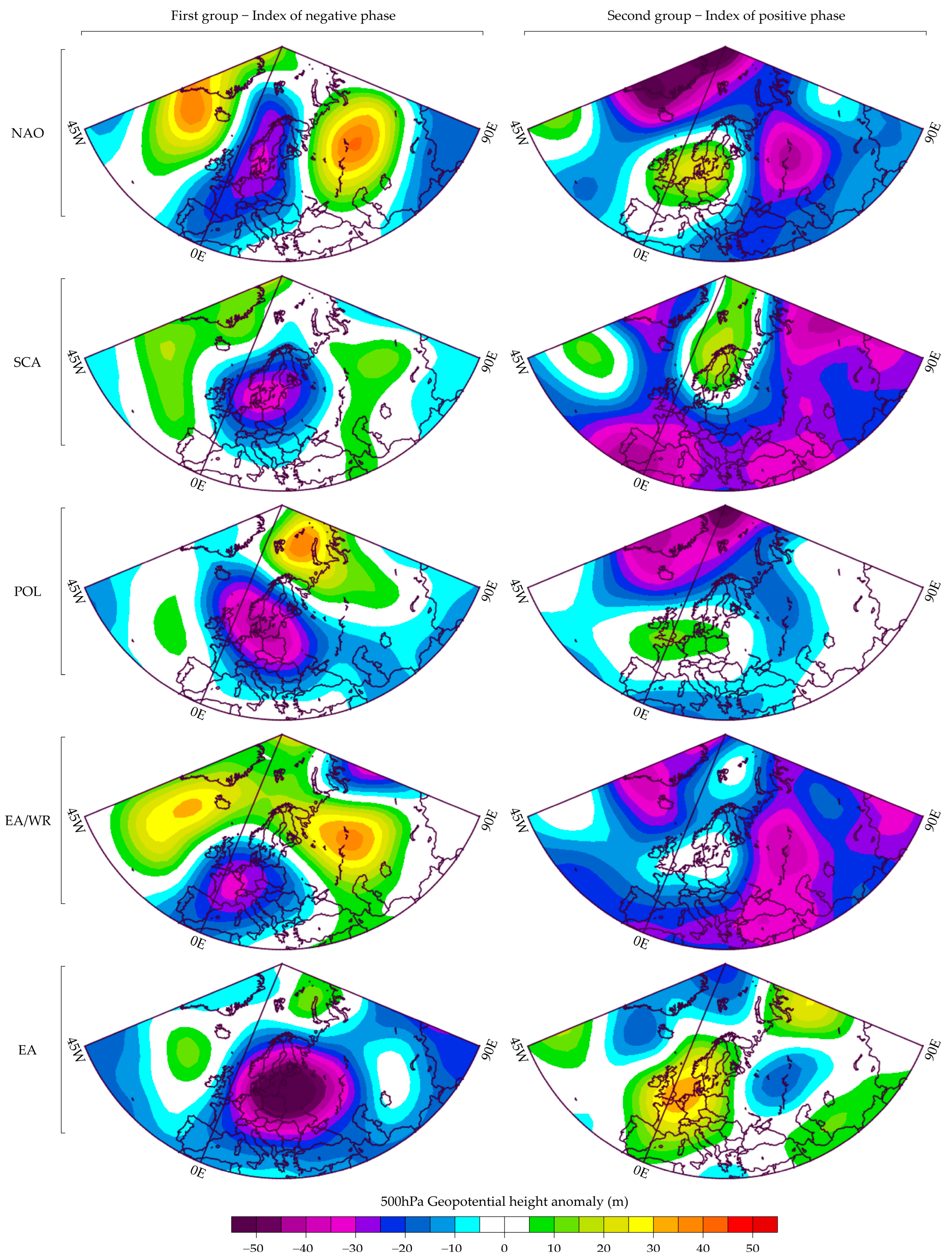
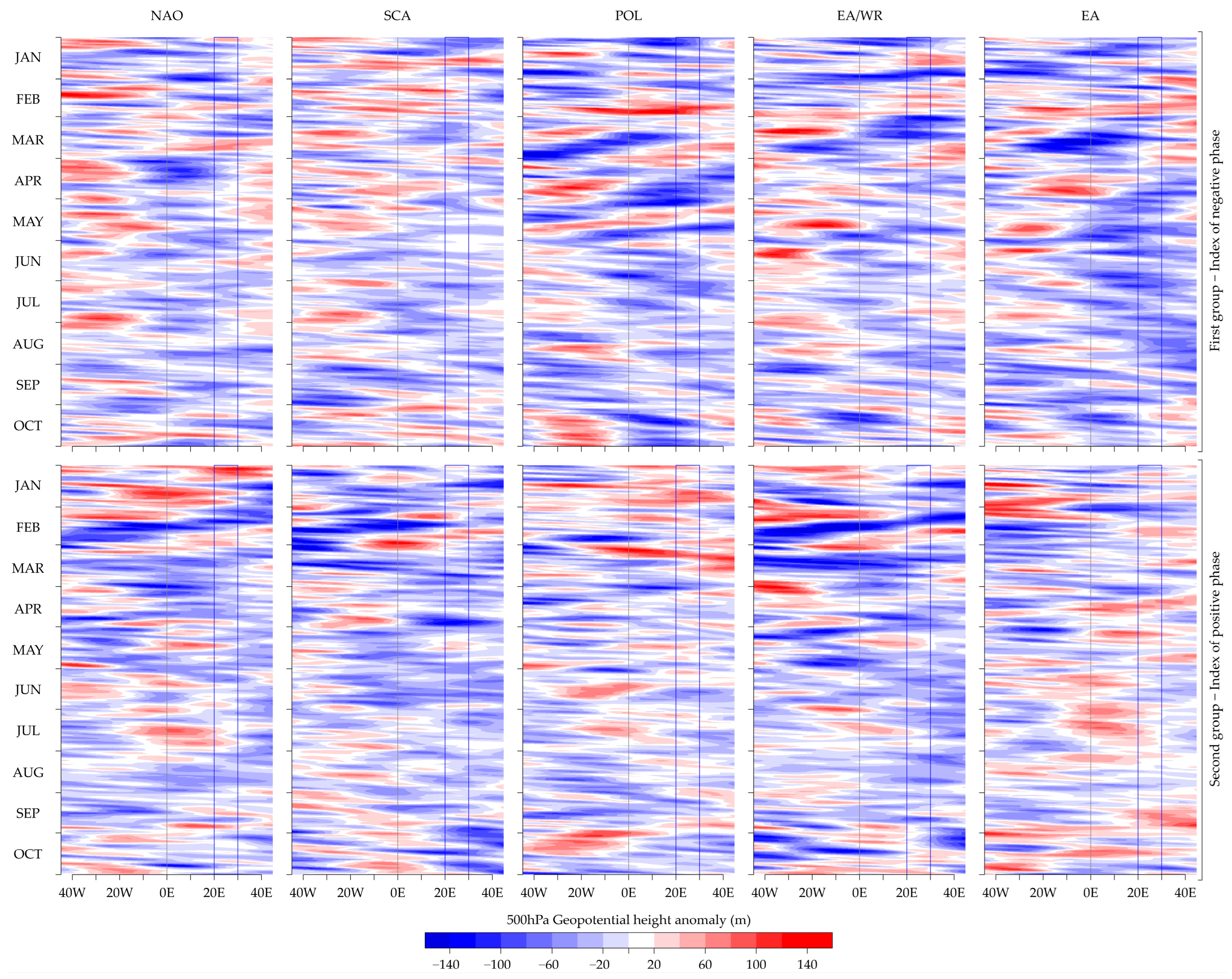
4.4. Atmospheric Circulation during the Low Flow

To determine the atmospheric circulation during low flow, the most dominant years of the rivers with statistically significant relations were selected to highlight differences in the formation of the Q30 magnitude. The previous results of the statistically significant relationships showed that the lowest Q30 values prevailed during positive indices and, conversely, the highest Q30 values prevailed during negative indices. The produced 500 hPa geopotential height (Z500) anomaly maps showed the main differences in atmospheric circulation in the years with the highest and the lowest Q30 values (Figure 6). The maps showed that negative Z500 anomalies of up to 30–45 m above the study area were observed during the highest Q30 values, i.e., they fell in the years of the first group—indices of the negative phase. The central parts of the anomalies were mainly located over the southern part of the Baltic Sea and southern Scandinavia for the NAO, SCA, and POL indices. Moreover, the spread of the negative anomaly extended over the whole of Northern Europe, while the study area was located on the eastern periphery. In the case of the EA/WA index, the negative anomaly of Z500 was located over Western Europe with a large spatial extent. In the current situation, Lithuania was located in the north-eastern part of the observed anomaly. The distribution of the pressure gradients among the NAO and EA/WR indices showed a clear distribution and interaction of the anticyclonic circulation centres over the North Atlantic and West Siberia with the cyclonic centres over Western and Northern Europe. The strongest negative anomaly of Z500 was found for the EA index and reached up to 60 m. The central part of this anomaly coincided with the study area in the south-eastern part of the Baltic Sea region and covered almost all of Northern, Central, and Eastern Europe, with a negative anomaly of more than 20 m. These negative anomalies caused the presence of a cyclonic circulation that brought excess moisture to the target region. Due to its location in Eastern Europe, most of the incoming air masses were expected from the south. At the same time, the lowest Q30 values were observed during the positive phases of the indices. Accordingly, the maps of the Z500 anomalies showed the opposite regularities to those of the negative phases, because the positive Z500 anomalies were fixed over the study area. However, the anomalies were not very pronounced, as, on average, only 15–20 m anomalies were detected for the NAO, SCA, and POL indices. Especially for the EA/WR index, the anomaly maps indicated almost regular perennial Z500 conditions for the analysed region. The highest positive Z500 anomaly was again found for the EA index, when an anomaly of up to 35 m was found over Western Europe, which included all surrounding areas in its area of influence. In most cases, the study area was located in the eastern or south-eastern part of the positive Z500 anomaly, which determined blocking conditions for moisture transfer from the west. Moreover, such conditions cause relatively cool and dry air transfer from northern latitudes.
In addition, the heatmaps of the changes in the Z500 anomalies since the beginning of the year were created to indicate the main temporal development patterns for the two groups of years over time and zonal direction (Figure 7). The averaged 40–60° N latitude anomaly showed the main distribution of positive and negative Z500 anomalies for each selected index. In the years of the first group with the highest Q30 values, the positive Z500 anomaly dominated over the North Atlantic between 45 W and 10 W longitude compared to the years of the second group in most months of the warm season. This regularity caused predominant negative anomalies of Z500 and the subsequent cyclonic circulation eastward from 0 E and especially in the analysed region between 20 E and 30 E longitude. The POL and EA indices differed by the contrast in the Z500 anomalies between February and May for the first group years. There was an intense circulation within the region of the mentioned indices during the high low flow values. On the other hand, the lowest Q30 values were found during the years of the second group with low contrast and amplitude anomalies over the North Atlantic (between 45 W and 10 W longitude). Most of the obtained anomalies were relatively low and more cases of negative anomalies were detected than in the years of the first group. Consequently, more positive anomalies of the Z500 between 0 E and 30 E longitude were found in the years of the second group. The temporal development scales of the NAO, SCA, and EA/WR indices indicated a strong contrast between positive and negative Z500 anomalies for the January–March period during the low Q30 values.

5. Discussion

This study investigated the important area of understanding the complex interplay between teleconnection patterns and low flows in lowland rivers. Teleconnection indices, consisting of NAO, SCA, POL, EA/WR, and EA, have often been used as indicators of climate variability in scientific studies and selected to test certain hypotheses based on physical processes. The results of this study revealed remarkable relations between these teleconnection patterns and the annual values of Q30, while not exceptionally robust, show clear patterns of significant response. In most cases, the indices show negative correlations with Q30 values, with the exception of the SCA index for longer accumulation periods. On average, all indices show relatively weak correlations between the different accumulation scenarios. However, the non-parametric Wilcoxon–Mann–Whitney test revealed a strong Q30 response to the EA/WR climate index, as 20 out of 25 analysed WGS showed statistically significant relationships at least once per applied accumulative delay period. Moreover, the NAO index also had a strong influence. The character of the obtained relation was reflected by lower values of Q30 during the positive phase of the indices and vice versa. This is consistent with previous studies that have frequently found correlations between river discharge and the NAO in different regions of Europe [54,55]. Significant correlations, especially between 1973 and 1998, were observed for rivers in the Iberian Peninsula, with values of −0.76 for the Douro, −0.77 for the Tagus, and −0.79 for the Guadiana. These correlations were consistently higher than in previous decades, as noted by Trigo et al. [55]. In Lithuania, the development of dry periods was related to the negative NAO/AO phase and it was concluded that the sustained phase of dry periods appears to be less dependent on anomalous atmospheric circulations [56]. The seasonal dependence was noted by Giuntoli et al. [57], as the seasonal climate indices show a delay period, so that the summer hydrological droughts of northern France are linked to the NAO index of previous seasons. Accordingly, different delay periods should be taken into account in the search for interrelations. In the south-eastern Baltic Sea catchment, Wrzesiński and Paluszkiewicz [58] found significant positive correlations between the NAO and river discharge in the winter season, in contrast to negative correlations in the spring. Furthermore, Birsan [28] discovered strong negative correlations between the NAO (December–March) and the mean annual runoff in Romania, highlighting the role of large-scale atmospheric circulation and the orographic effects of the Carpathian Mountains. Jalón-Rojas and Castelle [59] investigated the influence of large-scale climate variability on winter river discharge in Western Europe. The strongest correlations were found with the NAO index, especially in the far northern regions (with correlation coefficients of up to 0.56) and in the southern latitudes (with only 0.72).
Based on the correlations between precipitation and atmospheric circulation, this study found that the NAO and EA/WR show a relatively stronger correlation with precipitation during the warm season than do the other indices. These correlations were influenced by the chosen accumulation period, with the NAO showing the strongest negative correlations during the summer months, particularly June, July, and August. The EA/WR index had the strongest negative correlations in August. These results agree with those of Sukhonos and Vyshkvarkova [60]. The AO and NAO have a greater influence on the extremes in winter (positive correlation), while the EA/WR pattern has a greater influence on the region in summer and has a negative correlation. The results of Burt and Howden [61] are consistent with previous studies showing a remarkable positive correlation between precipitation in mountainous regions and the NAO in autumn, winter, and spring. Conversely, there is a clear negative correlation in the English lowlands in summer. In Serbia, the dominance of the NAO in winter, EA/WR in autumn, and EA in all seasons for cold–dry and warm–dry conditions were emphasised [62]. Devi et al. [63] developed a simple seasonal forecast model for the prediction of winter precipitation and found a significant negative correlation of −0.57 with the NAO. Significant positive correlations were also found between EA/WR and cold–dry conditions in autumn and negative correlations between EA/WR and warm–dry conditions in summer. However, some studies have provided results that despite the strong correlation between rainfall and river discharge, no significant correlations were found between precipitation over northern Spain and the NAO index [64].
The geopotential height anomalies maps of the 500 mb isobaric surface (Z500) showed that at high Q30 values, the negative Z500 anomalies of 30–45 m prevailed in the southern part of the Baltic Sea and extended over Northern Europe in the case of the NAO, SCA, and POL indices. In the case of EA-WR, the negative Z500 anomaly was observed over Central Europe (eastern France), but the north-eastern edge covered the study area. At low Q30 values, positive Z500 anomalies prevailed, but they were not as pronounced as in the previously discussed case and averaged 15–20 m in the central parts. However, they were sufficient to have a reducing effect on the Q30 size. In the southern Baltic Sea region, the composite analysis of 500 hPa geopotential height anomalies during dry periods showed different patterns, from weak high-pressure gradients to mild cyclonic circulations [56]. In the longest dry episodes in Lithuania, there was a distinct pattern at the 500 hPa level with a positive anomaly up to 90 m over Scandinavia and a negative centre over Western Europe, the Mediterranean, and the Balkans. This indicates that anticyclones over Scandinavia cause persistent precipitation deficits in Lithuania [56]. It is comparable to the summer Scandinavian blocking high and the positive phase of the Scandinavian teleconnection pattern, although it is less pronounced in summer [65,66]. Analysing the role of teleconnection patterns in the variability and trends of growing season indices across Europe revealed very similar trends [67]. In summer, the NAO weakens and shifts northwards, while the positive SCA phase reduces precipitation in Scandinavia and increases it over the north-eastern Atlantic. In the positive EA/WR phase, the height anomalies are positive over the North Sea and Mongolia and negative over Western Russia, resulting in southerly winds in winter and northerly winds from April to October in Eastern Europe. The same was confirmed by Ionita [32], who showed that the EA/WR is strongest in winter, with a positive EA/WR phase associated with dry conditions in Southern Europe and heavier precipitation over Scandinavia, as well as higher temperatures over Northern and Central Europe but cooler temperatures over Southern Europe. Lim [68] also confirmed that the negative EA/WR phase is associated with cooler temperatures in Western Europe and warmer temperatures in Eastern Europe. In the Mediterranean, especially in the western and northern regions, the positive phase of the EA oscillation contributes to dry and warm months associated with subtropical conditions [69]. Conversely, the negative mode of the EA favours wet and cold months, especially in the northern and western parts of the basin. The EA/WR oscillation effectively predicts dry–warm and wet–cold events in the eastern Mediterranean. In addition, Putniković et al. [70] found a consistently negative correlation between the EA/WR index and the geopotential height at 500 hPa over Russia, north of the Caspian Sea, throughout the year. The strongly negative EA/WR phase corresponded to positive temperature anomalies in Eastern Europe, while the strongly positive phase led to below-average temperatures.
This study addresses the complex interplay between teleconnection patterns and the behaviour of lowland rivers, focusing on the influence of atmospheric circulation indices as drivers of the parameters of potential ecological flow. This analysis reveals remarkable relations between selected teleconnection patterns and annual Q30 values, showing a consistent response. The relations showed negative associations with Q30 values, especially the Q30 connection with the EA/WR index. Based on these results, future research could focus on the genesis of individual low flow events, paying additional attention to macrocirculation patterns that would indicate the precise development of target events. In essence, this study highlights the crucial role of teleconnection patterns in the formation of low flow and the response of lowland rivers to climate variability and provides valuable insights for further research and forecasting efforts.

6. Conclusions

This study investigated the relationships between five atmospheric teleconnection patterns (NAO, SCA, POL, EA/WR, and EA) and the average minimum discharge of the 30 driest continuous days in the warm season (Q30). Statistical analysis using the Wilcoxon–Mann–Whitney test investigated significant relationships between low flow and atmospheric circulation under different accumulative delay scenarios. The results revealed clear patterns between the selected teleconnections and the annual values of Q30. The EA/WR had the strongest interaction with Q30 regardless of temporal delay. Even 20 out of 25 WGSs showed statistically significant responses to the EA/WR index by the analysed scenarios. Most WGSs responded to the 3-month accumulative delay before the Q30 event. Meanwhile, the NAO and SCA showed a weaker impact on Q30, especially in the group of WGS of the Neris and Šventoji rivers for the 4-month accumulative delay. The POL index demonstrated a strong impact on Q30 only for the longer 6-month accumulation period. The general tendencies disclosed that the lowest Q30 values prevailed during the positive phases of the climate indices. These conditions were determined by the prevailing of anticyclonic circulation, as the analysed region was located at the eastern edge of the positive geopotential height anomalies of the 500 hPa isobar surface. Accordingly, the eastern edge of obtained anomalies played a crucial role in the formation of Q30 with respect to climate indices that caused the anomalies of such shape. Conversely, the highest Q30 values and their larger dispersion were observed during the negative phases of the analysed climate indices when the negative geopotential height anomalies dominated over the study area.

Author Contributions

Conceptualization, K.G. and V.A.; methodology, K.G. and V.A.; formal analysis, K.G., V.A. and D.M.-L.; investigation, K.G. and V.A.; writing—original draft preparation, K.G., V.A. and D.M.-L.; writing—review and editing, K.G., V.A. and D.M.-L.; visualization, K.G. and V.A. All authors have read and agreed to the published version of the manuscript.

Funding

This research received no external funding.

Data Availability Statement

The data that support the findings of this study are available from the paper authors upon reasonable request.

Acknowledgments

NCEP–NCAR Reanalysis 1 data provided by the NOAA Physical Sciences Laboratory, Boulder, Colorado, USA, from their website at https://psl.noaa.gov (last accessed on 6 November 2023) for Z500 anomaly maps.

Conflicts of Interest

The authors declare no conflict of interest.

References

  1. Whitehead, P.G.; Wilby, R.L.; Battarbee, R.W.; Kernan, M.; Wade, A.J. A Review of the Potential Impacts of Climate Change on Surface Water Quality. Hydrol. Sci. J. 2009, 54, 101–123. [Google Scholar] [CrossRef]
  2. Merga, D.D.; Adeba, D.; Regasa, M.S.; Leta, M.K. Evaluation of Surface Water Resource Availability under the Impact of Climate Change in the Dhidhessa Sub-Basin, Ethiopia. Atmosphere 2022, 13, 1296. [Google Scholar] [CrossRef]
  3. Banerjee, D.; Ganguly, S. A Review on the Research Advances in Groundwater–Surface Water Interaction with an Overview of the Phenomenon. Water 2023, 15, 1552. [Google Scholar] [CrossRef]
  4. Schneider, C.; Laizé, C.L.R.; Acreman, M.C.; Flörke, M. How Will Climate Change Modify River Flow Regimes in Europe? Hydrol. Earth Syst. Sci. 2013, 17, 325–339. [Google Scholar] [CrossRef]
  5. Pardo-Loaiza, J.; Solera, A.; Bergillos, R.J.; Paredes-Arquiola, J.; Andreu, J. Improving Indicators of Hydrological Alteration in Regulated and Complex Water Resources Systems: A Case Study in the Duero River Basin. Water 2021, 13, 2676. [Google Scholar] [CrossRef]
  6. Dahal, N.; Shrestha, U.; Tuitui, A.; Ojha, H. Temporal Changes in Precipitation and Temperature and Their Implications on the Streamflow of Rosi River, Central Nepal. Climate 2018, 7, 3. [Google Scholar] [CrossRef]
  7. Kadir, M.; Fehri, R.; Souag, D.; Vanclooster, M. Exploring Causes of Streamflow Alteration in the Medjerda River, Algeria. J. Hydrol. Reg. Stud. 2020, 32, 100750. [Google Scholar] [CrossRef]
  8. Blöschl, G.; Hall, J.; Parajka, J.; Perdigão, R.A.P.; Merz, B.; Arheimer, B.; Aronica, G.T.; Bilibashi, A.; Bonacci, O.; Borga, M.; et al. Changing Climate Shifts Timing of European Floods. Science 2017, 357, 588–590. [Google Scholar] [CrossRef]
  9. Mentaschi, L.; Alfieri, L.; Dottori, F.; Cammalleri, C.; Bisselink, B.; Roo, A.D.; Feyen, L. Independence of Future Changes of River Runoff in Europe from the Pathway to Global Warming. Climate 2020, 8, 22. [Google Scholar] [CrossRef]
  10. Grizzetti, B.; Pistocchi, A.; Liquete, C.; Udias, A.; Bouraoui, F.; Van De Bund, W. Human Pressures and Ecological Status of European Rivers. Sci. Rep. 2017, 7, 205. [Google Scholar] [CrossRef]
  11. Pichura, V.; Potravka, L.; Skrypchuk, P.; Stratichuk, N. Anthropogenic and Climatic Causality of Changes in the Hydrological Regime of the Dnieper River. J. Ecol. Eng. 2020, 21, 1–10. [Google Scholar] [CrossRef] [PubMed]
  12. Ekka, A.; Pande, S.; Jiang, Y.; Der Zaag, P.V. Anthropogenic Modifications and River Ecosystem Services: A Landscape Perspective. Water 2020, 12, 2706. [Google Scholar] [CrossRef]
  13. Rahmonov, O.; Dragan, W.; Cabała, J.; Krzysztofik, R. Long-Term Vegetation Changes and Socioeconomic Effects of River Engineering in Industrialized Areas (Southern Poland). Int. J. Environ. Res. Public Health 2023, 20, 2255. [Google Scholar] [CrossRef] [PubMed]
  14. Shi, X.; Qin, T.; Nie, H.; Weng, B.; He, S. Changes in Major Global River Discharges Directed into the Ocean. Int. J. Environ. Res. Public Health 2019, 16, 1469. [Google Scholar] [CrossRef] [PubMed]
  15. Sofia, G.; Nikolopoulos, E.I. Floods and Rivers: A Circular Causality Perspective. Sci. Rep. 2020, 10, 5175. [Google Scholar] [CrossRef] [PubMed]
  16. Depetris, P.J. The Importance of Monitoring River Water Discharge. Front. Water 2021, 3, 745912. [Google Scholar] [CrossRef]
  17. Galster, J.C. Natural and Anthropogenic Influences on the Scaling of Discharge with Drainage Area for Multiple Watersheds. Geosphere 2007, 3, 260. [Google Scholar] [CrossRef]
  18. Wolf, S.; Esser, V.; Schüttrumpf, H.; Lehmkuhl, F. Influence of 200 Years of Water Resource Management on a Typical Central European River. Does Industrialization Straighten a River? Environ. Sci. Eur. 2021, 33, 15. [Google Scholar] [CrossRef]
  19. De Beurs, K.M.; Henebry, G.M.; Owsley, B.C.; Sokolik, I.N. Large Scale Climate Oscillation Impacts on Temperature, Precipitation and Land Surface Phenology in Central Asia. Environ. Res. Lett. 2018, 13, 065018. [Google Scholar] [CrossRef]
  20. Fu, W.; Steinschneider, S. A Diagnostic-Predictive Assessment of Winter Precipitation over the Laurentian Great Lakes: Effects of ENSO and Other Teleconnections. J. Hydrometeorol. 2019, 20, 117–137. [Google Scholar] [CrossRef]
  21. Graf, R.; Wrzesiński, D. Relationship between Water Temperature of Polish Rivers and Large-Scale Atmospheric Circulation. Water 2019, 11, 1690. [Google Scholar] [CrossRef]
  22. Manzano, A.; Clemente, M.A.; Morata, A.; Luna, M.Y.; Beguería, S.; Vicente-Serrano, S.M.; Martín, M.L. Analysis of the Atmospheric Circulation Pattern Effects over SPEI Drought Index in Spain. Atmospheric Research 2019, 230, 104630. [Google Scholar] [CrossRef]
  23. Plewa, K.; Perz, A.; Wrzesiński, D. Links between Teleconnection Patterns and Water Level Regime of Selected Polish Lakes. Water 2019, 11, 1330. [Google Scholar] [CrossRef]
  24. Massei, N.; Kingston, D.G.; Hannah, D.M.; Vidal, J.-P.; Dieppois, B.; Fossa, M.; Hartmann, A.; Lavers, D.A.; Laignel, B. Understanding and Predicting Large-Scale Hydrological Variability in a Changing Environment. Proc. Int. Assoc. Hydrol. Sci. 2020, 383, 141–149. [Google Scholar] [CrossRef]
  25. Jiang, Q.; Cioffi, F.; Giannini, M.; Wang, J.; Li, W. Analysis of Changes in Large-scale Circulation Patterns Driving Extreme Precipitation Events over the c entral-eastern China. Int. J. Climatol. 2023, 43, 519–537. [Google Scholar] [CrossRef]
  26. Ionita, M.; Boroneanṭ, C.; Chelcea, S. Seasonal Modes of Dryness and Wetness Variability over Europe and Their Connections with Large Scale Atmospheric Circulation and Global Sea Surface Temperature. Clim. Dyn. 2015, 45, 2803–2829. [Google Scholar] [CrossRef]
  27. Pandžić, K.; Likso, T.; Trninić, D.; Oskoruš, D.; Macek, K.; Bonacci, O. Relationships between Large-Scale Atmospheric Circulation and Monthly Precipitation and Discharge in the Danube River Basin. Theor. Appl. Climatol. 2022, 148, 767–777. [Google Scholar] [CrossRef]
  28. Birsan, M.-V. Trends in Monthly Natural Streamflow in Romania and Linkages to Atmospheric Circulation in the North Atlantic. Water Resour. Manage. 2015, 29, 3305–3313. [Google Scholar] [CrossRef]
  29. Wang, W.; Yang, P.; Xia, J.; Zhang, S.; Cai, W. Coupling Analysis of Surface Runoff Variation with Atmospheric Teleconnection Indices in the Middle Reaches of the Yangtze River. Theor. Appl. Climatol. 2022, 148, 1513–1527. [Google Scholar] [CrossRef]
  30. Lorenzo-Lacruz, J.; Morán-Tejeda, E.; Vicente-Serrano, S.M.; Hannaford, J.; García, C.; Peña-Angulo, D.; Murphy, C. Streamflow Frequency Changes across Western Europe and Interactions with North Atlantic Atmospheric Circulation Patterns. Global Planet. Chang. 2022, 212, 103797. [Google Scholar] [CrossRef]
  31. Girjatowicz, J.P.; Świątek, M. Effects of Atmospheric Circulation on Water Temperature along the Southern Baltic Sea Coast. Oceanologia 2019, 61, 38–49. [Google Scholar] [CrossRef]
  32. Ionita, M. The Impact of the East Atlantic/Western Russia Pattern on the Hydroclimatology of Europe from Mid-Winter to Late Spring. Climate 2014, 2, 296–309. [Google Scholar] [CrossRef]
  33. Ionita, M. Interannual Summer Streamflow Variability over Romania and Its Connection to Large-scale Atmospheric Circulation. Int. J. Climatol. 2015, 35, 4186–4196. [Google Scholar] [CrossRef]
  34. Bierkens, M.F.P.; Van Beek, L.P.H. Seasonal Predictability of European Discharge: NAO and Hydrological Response Time. J. Hydrometeorol. 2009, 10, 953–968. [Google Scholar] [CrossRef]
  35. Kingston, D.G.; Lawler, D.M.; McGregor, G.R. Linkages between Atmospheric Circulation, Climate and Streamflow in the Northern North Atlantic: Research Prospects. Prog. Phys. Geogr. Earth Environ. 2006, 30, 143–174. [Google Scholar] [CrossRef]
  36. Bouwer, L.M.; Vermaat, J.E.; Aerts, J.C.J.H. Winter Atmospheric Circulation and River Discharge in Northwest Europe. Geophys. Res. Lett. 2006, 33, 2005GL025548. [Google Scholar] [CrossRef]
  37. Bouwer, L.M.; Vermaat, J.E.; Aerts, J.C.J.H. Regional Sensitivities of Mean and Peak River Discharge to Climate Variability in Europe. J. Geophys. Res. 2008, 113, 2008JD010301. [Google Scholar] [CrossRef]
  38. Montaldo, N.; Sarigu, A. Potential Links between the North Atlantic Oscillation and Decreasing Precipitation and Runoff on a Mediterranean Area. J. Hydrol. 2017, 553, 419–437. [Google Scholar] [CrossRef]
  39. Phillips, I.D.; McGregor, G.R.; Wilson, C.J.; Bower, D.; Hannah, D.M. Regional Climate and Atmospheric Circulation Controls on the Discharge of Two British Rivers, 1974–1997. Theor. Appl. Climatol. 2003, 76, 141–164. [Google Scholar] [CrossRef]
  40. Irannezhad, M.; Torabi Haghighi, A.; Chen, D.; Kløve, B. Variability in Dryness and Wetness in Central Finland and the Role of Teleconnection Patterns. Theor. Appl. Climatol. 2015, 122, 471–486. [Google Scholar] [CrossRef]
  41. Uvo, C.B.; Foster, K.; Olsson, J. The Spatio-Temporal Influence of Atmospheric Teleconnection Patterns on Hydrology in Sweden. J. Hydrol. Reg. Stud. 2021, 34, 100782. [Google Scholar] [CrossRef]
  42. Stahl, K.; Demuth, S. Linking Streamflow Drought to the Occurrence of Atmospheric Circulation Patterns. Hydrol. Sci. J. 1999, 44, 467–482. [Google Scholar] [CrossRef]
  43. Šarauskienė, D.; Akstinas, V.; Nazarenko, S.; Kriaučiūnienė, J.; Jurgelėnaitė, A. Impact of Physico-geographical Factors and Climate Variability on Flow Intermittency in the Rivers of Water Surplus Zone. Hydrol. Process. 2020, 34, 4727–4739. [Google Scholar] [CrossRef]
  44. Nazarenko, S.; Meilutytė-Lukauskienė, D.; Šarauskienė, D.; Kriaučiūnienė, J. Spatial and Temporal Patterns of Low-Flow Changes in Lowland Rivers. Water 2022, 14, 801. [Google Scholar] [CrossRef]
  45. Akstinas, V.; Virbickas, T.; Kriaučiūnienė, J.; Šarauskienė, D.; Jakimavičius, D.; Rakauskas, V.; Negro, G.; Vezza, P. The Combined Impact of Hydropower Plants and Climate Change on River Runoff and Fish Habitats in Lowland Watersheds. Water 2021, 13, 3508. [Google Scholar] [CrossRef]
  46. Virbickas, T.; Vezza, P.; Kriaučiūnienė, J.; Akstinas, V.; Šarauskienė, D.; Steponėnas, A. Impacts of Low-Head Hydropower Plants on Cyprinid-Dominated Fish Assemblages in Lithuanian Rivers. Sci. Rep. 2020, 10, 21687. [Google Scholar] [CrossRef] [PubMed]
  47. Kim, Y.-W.; Lee, J.-W.; Woo, S.-Y.; Lee, J.-J.; Hur, J.-W.; Kim, S.-J. Design of Ecological Flow (E-Flow) Considering Watershed Status Using Watershed and Physical Habitat Models. Water 2023, 15, 3267. [Google Scholar] [CrossRef]
  48. Leone, M.; Gentile, F.; Lo Porto, A.; Ricci, G.F.; De Girolamo, A.M. Ecological Flow in Southern Europe: Status and Trends in Non-Perennial Rivers. J. Environ. Manag. 2023, 342, 118097. [Google Scholar] [CrossRef]
  49. Barnston, A.G.; Livezey, R.E. Classification, Seasonality and Persistence of Low-Frequency Atmospheric Circulation Patterns. Mon. Wea. Rev. 1987, 115, 1083–1126. [Google Scholar] [CrossRef]
  50. Gailiušis, B.; Jablonskis, J.; Kovalenkovienė, M. The Lithuanian Rivers. Hydrography and Runoff; Lithuanian Energy Institute: Kaunas, Lithuania, 2001; p. 796. (In Lithuanian) [Google Scholar]
  51. Lithuanian Hydrometeorological Service under the Ministry of Environment. Assessment of climate changes in Lithuania comparing 1961–1990 and 1991–2020 Climatological Normal; LHMT Climate and Research Department: Vilnius, Lithuania, 2021; p. 18. (In Lithuanian) [Google Scholar]
  52. Akstinas, V.; Šarauskienė, D.; Kriaučiūnienė, J.; Nazarenko, S.; Jakimavičius, D. Spatial and Temporal Changes in Hydrological Regionalization of Lowland Rivers. Int. J. Environ. Res. 2022, 16, 1. [Google Scholar] [CrossRef]
  53. Fay, M.P.; Proschan, M.A. Wilcoxon-Mann-Whitney or t-Test? On Assumptions for Hypothesis Tests and Multiple Interpretations of Decision Rules. Stat. Surv. 2010, 4, 1–39. [Google Scholar] [CrossRef] [PubMed]
  54. Lorenzo-Lacruz, J.; Vicente-Serrano, S.M.; López-Moreno, J.I.; González-Hidalgo, J.C.; Morán-Tejeda, E. The Response of Iberian Rivers to the North Atlantic Oscillation. Hydrol. Earth Syst. Sci. 2011, 15, 2581–2597. [Google Scholar] [CrossRef]
  55. Trigo, R.M.; Pozo-Vázquez, D.; Osborn, T.J.; Castro-Díez, Y.; Gámiz-Fortis, S.; Esteban-Parra, M.J. North Atlantic Oscillation Influence on Precipitation, River Flow and Water Resources in the Iberian Peninsula. Int. J. Climatol. 2004, 24, 925–944. [Google Scholar] [CrossRef]
  56. Rimkus, E.; Kažys, J.; Valiukas, D.; Stankūnavičius, G. The atmospheric circulation patterns during dry periods in Lithuania**The study was supported by the Lithuanian-Swiss cooperation programme to reduce economic and social disparities within the enlarged European Union under project agreement No. CH-3-ŠMM-01/05. Oceanologia 2014, 56, 223–239. [Google Scholar] [CrossRef]
  57. Giuntoli, I.; Renard, B.; Vidal, J.-P.; Bard, A. Low Flows in France and Their Relationship to Large-Scale Climate Indices. J. Hydrol. 2013, 482, 105–118. [Google Scholar] [CrossRef]
  58. Wrzesiński, D.; Paluszkiewicz, R. Spatial Differences in the Impact of the North Atlantic Oscillation on the Flow of Rivers in Europe. Hydrol. Res. 2011, 42, 30–39. [Google Scholar] [CrossRef]
  59. Jalón-Rojas, I.; Castelle, B. Climate Control of Multidecadal Variability in River Discharge and Precipitation in Western Europe. Water 2021, 13, 257. [Google Scholar] [CrossRef]
  60. Sukhonos, O.; Vyshkvarkova, E. Connection of Compound Extremes of Air Temperature and Precipitation with Atmospheric Circulation Patterns in Eastern Europe. Climate 2023, 11, 98. [Google Scholar] [CrossRef]
  61. Burt, T.P.; Howden, N.J.K. North Atlantic Oscillation Amplifies Orographic Precipitation and River Flow in Upland Britain: NAO Drives Double Orographic Enhancement. Water Resour. Res. 2013, 49, 3504–3515. [Google Scholar] [CrossRef]
  62. Arsenović, P.; Tošić, I.; Unkašević, M. Trends in Combined Climate Indices in Serbia from 1961 to 2010. Meteorol. Atmos Phys. 2015, 127, 489–498. [Google Scholar] [CrossRef]
  63. Devi, U.; Shekhar, M.S.; Singh, G.P.; Dash, S.K. Statistical Method of Forecasting of Seasonal Precipitation over the Northwest Himalayas: North Atlantic Oscillation as Precursor. Pure Appl. Geophys. 2020, 177, 3501–3511. [Google Scholar] [CrossRef]
  64. Aravena, G.; Villate, F.; Iriarte, A.; Uriarte, I.; Ibáñez, B. Influence of the North Atlantic Oscillation (NAO) on Climatic Factors and Estuarine Water Temperature on the Basque Coast (Bay of Biscay): Comparative Analysis of Three Seasonal NAO Indices. Cont. Shelf Res. 2009, 29, 750–758. [Google Scholar] [CrossRef]
  65. Cassou, C.; Terray, L.; Phillips, A.S. Tropical Atlantic Influence on European Heat Waves. J. Clim. 2005, 18, 2805–2811. [Google Scholar] [CrossRef]
  66. Bueh, C.; Nakamura, H. Scandinavian Pattern and Its Climatic Impact: Scandinavian Pattern and Its Climatic Impact. Q. J. R. Meteorol. Soc. A J. Atmos. Sci. Appl. Meteorol. Phys. Oceanogr. 2007, 133, 2117–2131. [Google Scholar] [CrossRef]
  67. Craig, P.M.; Allan, R.P. The Role of Teleconnection Patterns in the Variability and Trends of Growing Season Indices across Europe. Int. J. Climatol. 2022, 42, 1072–1091. [Google Scholar] [CrossRef]
  68. Lim, Y.-K. The East Atlantic/West Russia (EA/WR) Teleconnection in the North Atlantic: Climate Impact and Relation to Rossby Wave Propagation. Clim. Dyn. 2015, 44, 3211–3222. [Google Scholar] [CrossRef]
  69. Lemus-Canovas, M. Changes in Compound Monthly Precipitation and Temperature Extremes and Their Relationship with Teleconnection Patterns in the Mediterranean. J. Hydrol. 2022, 608, 127580. [Google Scholar] [CrossRef]
  70. Putniković, S.; Tošić, I.; Lazić, L.; Pejanović, G. The Influence of the Large-Scale Circulation Patterns on Temperature in Serbia. Atmos. Res. 2018, 213, 465–475. [Google Scholar] [CrossRef]
Figure 1. Spatial distribution of the selected WGSs and MSs.
Water 16 00066 g001
Figure 2. The correlations between Q30 and selected climate indices (NAO, SCA, POL, EA/WR, and EA) for all analysed WGSs according to different scenarios.
Water 16 00066 g002
Figure 3. Results of the Wilcoxon–Mann–Whitney test between Q30 and the studied climate indices (NAO, SCA, POL, EA/WR, and EA) for all selected WGSs according to different scenarios. The green boxes indicate that there is a borderline statistical relation (90%) or that the relationship is statistically significant (95% and 99%).
Water 16 00066 g003
Figure 4. Distribution of 20 standardised values of Q30 corresponding to negative phases of the studied index (a first rank, marked as purple bars) and 20 standardised values of Q30 corresponding to positive phases of the studied index (a second rank, marked as green bars). The Q30 value was normalised, taking into consideration the maximum Q30 value of each WGS. The row of purple/green bars inside each graph represents a river with a statistically significant relation (≥95%).
Water 16 00066 g004
Figure 5. Correlation between monthly precipitation and selected climate indices for different accumulation periods (1 to 6 months). A negative month value on the vertical axis indicates the month of the previous year.
Water 16 00066 g005
Figure 6. Spatial distribution of geopotential height anomalies of 500 hPa isobaric surface (generated by the NOAA PSL Monthly Composites application) during the warm season for the first (years with negative index phase and the highest Q30) and second (years with positive index phase and the lowest Q30) group years by selected climate indices.
Water 16 00066 g006
Figure 7. Temporal change in the anomalies of the geopotential height of the 500 hPa isobaric surface (based on data from the NOAA PSL Time Section Plots Using Gridded Daily Data application) over the year for the first (years with negative index phase and the highest Q30) and second (years with positive index phase and the lowest Q30) group years according to selected climate indices.
Water 16 00066 g007
Disclaimer/Publisher’s Note: The statements, opinions and data contained in all publications are solely those of the individual author(s) and contributor(s) and not of MDPI and/or the editor(s). MDPI and/or the editor(s) disclaim responsibility for any injury to people or property resulting from any ideas, methods, instructions or products referred to in the content.

