Abstract
Correcting the bias of satellite precipitation products (SPPs) based on ground rainfall observations is one effective approach to improve their performance. To date, there have been limited efforts in correcting the bias of hourly SPPs with mixed results. In this study, ratio bias correction (RBC) and probability density matching (PDF) are used to correct the bias of four hourly SPPs (GSMaP_NRT, IMERG_E, IMERG_L, and IMERG) based on ground rainfall observations in a hilly watershed, China. Furthermore, SWAT (Soil and Water Assessment Tool) models are developed using ground rainfall observations, original SPPs, and bias-corrected SPPs to simulate the daily streamflow at the Yuetan Hydrological Station so as to comprehensively compare the performance of the two bias correction methods and evaluate the potentials of the four hourly SPPs in hydrological modeling applications. Our study results show that both RBC and PDF could improve the accuracy of hourly SPPs to various degrees, with PDF outperforming RBC considerably. After being corrected by PDF, the CC values of the four SPPs all reached 0.65. In addition, the SWAT models utilizing the PDF-corrected SPPs simulated the daily streamflow at the Yuetan Station better than those utilizing the RBC-corrected SPPs. Specifically, PDF-corrected IMERG_F performed the best among the four hourly SPPs, with a R2 of 0.89, NSE of 0.89, and RB of −8.14%. After bias correction, hourly satellite precipitation products can be well applied to hydrological modeling in the region.
1. Introduction
As an essential part of the Earth’s hydrological cycle, precipitation serves as important data for meteorological and hydrological research [1]. Meanwhile, as a critical input variable for hydrological models, the accuracy of precipitation data directly affects the quality of simulation results [2]. Traditional precipitation data primarily come from ground-based measurements, which may have high accuracy but are susceptible to terrain influences and uneven spatial and temporal distributions. With the advantages of wide coverage, uniform spatial distribution, continuous temporal availability, and high temporal resolution, satellite precipitation products (SPPs) have gradually become an important data source for meteorological monitoring and hydrological simulations [3]. Tan et al. (2018) evaluated the accuracy of three GPM precipitation products (IMERG_E, IMERG_L, and IMERG_F) and then used them as precipitation inputs to SWAT (Soil and Water Assessment Tool, which is developed under the collaboration of the U.S. Department of Agriculture and the Texas A&M University, College Station, TX, USA) models to compare their streamflow simulation performance in the Kelantan River Basin of Malaysia. They concluded that all three SPPs could effectively capture precipitation variability in the region and yield a satisfactory performance in daily streamflow simulation. Furthermore, the SWAT model based on IMERG_F performed the best in simulating daily peak flows in the region [4].
However, as an indirect precipitation monitoring method, satellite precipitation estimation is subject to both systematic and random errors. Many studies have been conducted to evaluate the SPPs around the world, which have found significant differences in the accuracy of SPPs at different temporal scales across the regions [5,6,7,8,9,10]. The accuracy of SPPs could be affected by a variety of factors, such as the precipitation type, season, geographical location, land cover, and topography [11,12,13,14]. Furthermore, SPPs are generally capable of providing better daily or monthly precipitation estimates, whereas their hourly precipitation estimates are much less satisfactory [15,16,17,18,19]. For example, Xu et al. (2019) found an extremely weak correlation between the IMERG 05B and rain gauge measurement in mainland China with a coefficient of determination (R2) of less than 0.12 [17]. Yuan et al. (2019) compared the performance of five hourly SPPs in the Chindwin watershed of Myanmar and found that even the best hourly IMERG_F could merely yield a CC of 0.33 [19]. Hourly rainfall data are valuable for a variety of hydrological applications, such as flash flooding forecast and prevention in fast-responding catchments [20,21]. Previous studies have also demonstrated that the hydrological modeling performance could be improved by using sub-daily rainfall inputs [22,23]. Evidently, developing effective bias correction methods to improve their accuracy is indispensable to employing the hourly SPPs in hydrological applications.
Extensive research has been conducted on the bias correction of SPPs, and a variety of bias correction methods have been proposed, such as ratio bias correction [24], dual-core smoothing correction [25], cokriging method [26], probability matching method [27], Bayesian correction method [28], optimal interpolation–probability matching method [29], and integrated fusion through inverse error variance weighting [30]. To date, previous studies have been mostly limited to correcting the bias of SPPs at the daily scale, whereas few have been conducted at the hourly scale despite the generally poorer performance of hourly SPPs. The existing studies on the bias correction of hourly SPPs have also highlighted the difficulty involved in and the urgent need for more research in the field [31]. For example, Mastrantonas et al. (2019) [32] corrected the bias of CMOPRH_RT, GSMaP_NRT, IMERG_E, IMERG_L, and PERSIANN_CCS in the Ghost Rage Basin region of Japan at the temporal scales ranging from hourly to daily and monthly. They found that their bias correction methods improved the accuracy of all SPPs at the monthly and daily scales, but they were barely effective at the hourly scale.
In addition to using various statistical metrics, hydrological modeling has been increasingly utilized to compare the accuracy of SPPs and assess the performance of various bias correction methods [33,34,35]. In the Kashgar catchment in Xinjiang, China, Wang et al. (2020) [36] utilized daily SPPs, such as GSMaP, CHIRPS (Climate Hazards Group InfraRed Preconception with Station Data), 3B42, and SM2RAIN (Rainfall Estimation from Soil Moisture Observations), as rainfall inputs to establish hydrological SWAT (Soil and Water Assessment Tool) models. Their results showed that the SWAT model based on GSMaP performed the best in simulating the daily runoff. In another study, Mo et al. (2020) [37] used the GDA method to correct the bias of daily IMERG, and they found that the SWAT model based on the biased-corrected IMERG could simulate long-term runoff satisfactorily in the karst Xiajiahe catchment of China. To date, the hydrological assessment of SPPs has been largely confined to daily products, with few studies having been carried out on the hourly SPPs.
Located in Huangshan City, Eastern China, the Shuaishui watershed is the source of the Qiantang River. Recognized as one of the key ecological functional areas for biodiversity conservation and water conservation in China, the Shuaishui watershed serves as an important ecological barrier and strategic water source reserve for the downstream Yangtze River Delta region. Due to its complex mountainous terrain and large elevation drop, the distribution of rainfall stations is highly uneven in the region. With the advantages of continuous spatiotemporal coverage and easy accessibility, SPPs are of great application value in the Shuaishui watershed. This study aims to correct the bias of various hourly SPPs with two candidate methods, namely, ratio bias correction (RBC) and Probability Density Function Matching (PDF), based on ground rainfall observations in the hilly Shuaishui watershed. The bias correction performance of the two methods was assessed by comparing the hydrological simulation performance of the SWAT models, which were respectively established utilizing ground observations and bias-corrected SPPs as the hourly rainfall inputs.
2. Materials and Methods
2.1. Study Area
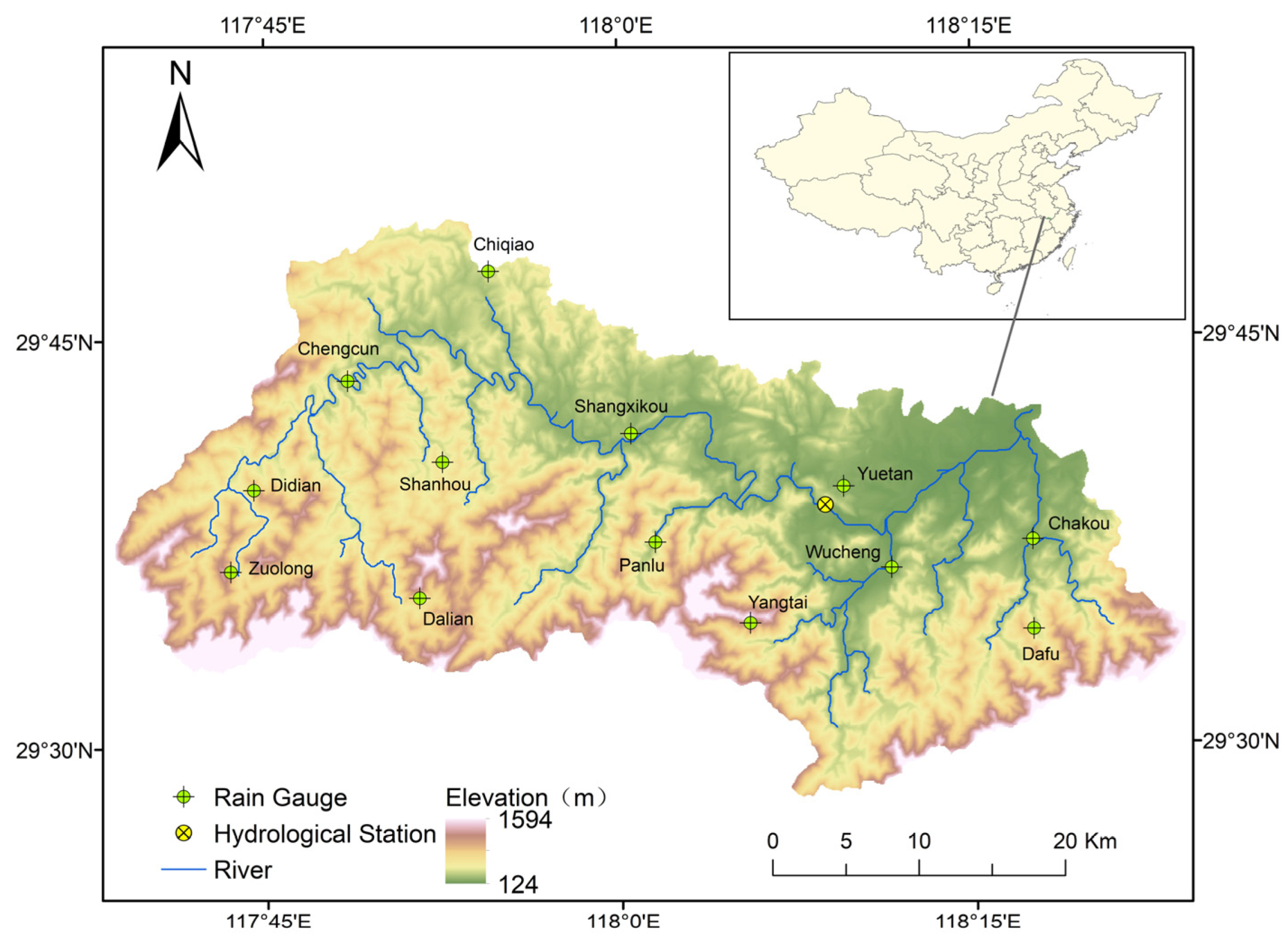
The Shuaishui watershed is located in the southern part of Anhui Province, Eastern China. With a total length of 159 km, the Shuaishui River originates from the Hutou Mountains and flows through three townships of Xiuning County in Huangshan City, namely, Liukou, Shangxikou, and Hongli, as well as two townships (Jianzhong and Liyang) in the Tunxi District. It eventually merges with the Hengjiang River at the Tunxi Bridge before flowing into the Xin’an River. Spanning coordinates from 117°39′ E to 119°26′ E and 29°24′ N to 31°10′ N, the Shuaishui watershed covers a total area of 1522 km2 (Figure 1).

Figure 1.
The Shuaishui watershed and the locations of ground rainfall stations.
The watershed receives abundant precipitation but with significant seasonal variations. In the rainy summer, the Shuaishui River is prone to rapid rises and falls during rainstorms, frequently leading to serious flood disasters [38]. For example, a severe flood occurred in June 2016 in the Shuaishui watershed, causing an economic loss of RMB 168 million [39].
2.2. Data Sources
2.2.1. Satellite Precipitation Products
Four satellite precipitation products (SPPs) from 1 January 2010 to 31 December 2017 were used in this study, including three versions of IMERG (Integrated Multi-Satellite Retrievals for Global Precipitation Measurement) (IMERG_E, IMERG_L, and IMERG_F) and the near-real-time product data (GSMaP_NRT) from the Global Satellite Mapping of Precipitation (GSMaP). All four SPPs have a spatial resolution of 0.1° × 0.1°. GSMaP_NRT has a temporal resolution of 1 h, while IMERG has a higher temporal resolution of 30 min, which was aggregated to 1 hour for subsequent hourly comparisons [40]. All SPPs were preprocessed to align them with the ground measurements. For example, the Coordinated Universal Times (UTCs) of the SPPs were converted to Beijing Time (UTC + 8 h) [41].
2.2.2. Meteorological and Hydrological Data
The daily meteorological data from 2010 to 2017 were obtained from the Tunxi Meteorological Station in Huangshan City, including solar radiation, wind speed, maximum and minimum temperature, and relative humidity. In addition, hourly rainfall at ten rain stations and daily streamflow at one hydrological station (Yuetan Station) during the same period were obtained from the Hydrological Yearbook of the People’s Republic of China (Table 1).

Table 1.
List of rainfall stations in the Shuaishui watershed.
2.2.3. Watershed Characteristics Data
The watershed characteristics data of the Shuaishui watershed mainly included digital elevation model (DEM), land use and land cover, soil type, and soil properties. Table 2 presents the details of the data and their sources.
Table 2.
Watershed characteristics data of the Shuaishui watershed.
2.3. Assessment of Hourly Satellite Precipitation Products
Four metrics were calculated to assess the performance of the hourly SPPs in the Shuaishui watershed, namely, the correlation coefficient (CC), relative bias (RB), root mean square error (RMSE), and mean absolute difference (MAD). Among them, CC was used to measure the temporal correlation between satellite precipitation estimates and ground rainfall observations. Its value ranged from −1 to 1, with an absolute value closer to 1 indicating a higher correlation. RB was used to measure the overall deviation of the satellite precipitation estimates from ground observations. An RB value near 0 indicated the 2 series were close; a positive RB indicates that SPPs overestimate ground precipitation, whereas a negative RB indicated an underestimation. The RMSE measured the average error between the satellite-derived precipitation estimates and ground-based observations, while MAD measured the difference between mean satellite precipitation estimates and mean ground observations. The closer the values of the RMSE and MAD were to 0, the higher the accuracy of the SPPs.
In addition, the Probability of Detection (POD), False Alarm Rate (FAR), and Critical Success Index (CSI) were computed to assess the hourly SPPs’ capacity to detect rainfall at 5 levels of rainfall intensities, namely, 0.1, 1, 5, 10, and 15 mm/h. The POD, which was calculated as the ratio of the number of correctly identified events by the SPPs to the total number of events, represented the percentage of rainfall events that the SPPs could correctly detect. A POD value closer to 1 indicated a higher hit rate for the SPPs. By dividing the number of improperly identified events with the total number of events, FAR showed the percentage of rainfall events that the SPPs incorrectly detected. An FAR value closer to 0 indicated fewer cases of incorrect detections by the SPPs. The CSI comprehensively reflected the degree of failed as well as false detections of rainfall events by the SPPs. The closer the CSI value was to 1, the stronger the overall rainfall detection capability of the SPPs [18].
2.4. Bias Correction of Hourly Satellite Participation Products
2.4.1. Ratio Bias Correction Method
The ratio bias correction (RBC) method has been widely used for correcting the bias of SPPs due to its simple calculation process. This method assumes that there is a similar bias between satellite precipitation estimates and ground rainfall observations across a space, and thereby corrects the satellite precipitation estimates by spatially extrapolating the bias calculated at individual ground locations. Based on its way of moving the temporal window, RBC can be classified into four types: BW (Backward Window), CW (Central Window), FW (Forward Window), and SW (Sequential Window) [42]. The first three types belong to the category of the sliding window, while the fourth type belongs to the category of the sequential window.
The multiplication bias ratio correction method [43] was used to correct the four hourly SPPs in the Shuaishui watershed, whose bias correction factors (BFs) were calculated with the following equations:
where Pg(i, t) and Ps(i, t), respectively, represent the hourly precipitation level at time t at the i-th rainfall station and the corresponding satellite precipitation estimate; l is the length of the temporal window; and m represents the number of hours considered before or after time t in the temporal window. Equation (1) is applicable to both CW and SW, while Equations (2) and (3) are, respectively, applicable to FW and BW.
The main steps of the RBC are as follows: (1) set the temporal window and calculate the ratio (BF) between the accumulated amount of ground rainfall and satellite precipitation estimates within the temporal window at each rainfall station; (2) spatially interpolate the BF values with the Inverse Distance Weighted (IDW) method; (3) multiply the original satellite precipitation estimates with the corresponding BF to obtain the corrected value; and (4) move the temporal window and repeat steps (1)–(3) until the end of the study period (2010–2017). An RBC with temporal windows differing in types (BW, CW, FW, and SW) and sizes (ranging from 3 to 25 h with a 2 h increment) was performed to correct the bias of the hourly SPPs in the Shuaishui watershed, whose bias correction performances were then compared to determine the optimal window.
2.4.2. Probability Density Function Matching Method
The Probability Density Function Matching (PDF) method has frequently been used for the bias correction of SPPs. It mainly eliminates the systematic bias in a satellite precipitation estimate by matching its cumulative distribution function (CDF) with that of ground rainfall observations within the defined temporal window.
The main steps of the PDF bias correction are as follows: (1) set the temporal window to be 30 days, or 720 h, preceding the current time to ensure that there is a sufficient amount of precipitation data to derive a stable CDF; (2) derive the CDFs of both ground rainfall and corresponding satellite precipitation estimates at each rainfall station, which are used to adjust the satellite precipitation estimates; (3) calculate the difference between original and adjusted satellite precipitation estimates at each station (ΔP = Psi − Psci); (4) spatially interpolate ΔP using the IDW method, and add the interpolated ΔP to the original satellite precipitation estimates to generate the PDF-corrected amount; and (5) repeat steps (2)–(4) for each temporal window till the end of the study period.
2.5. Bias Correction Performance Evaluation
2.5.1. Cross-Validation
Cross-validation (CV) was performed to assess the effectiveness of the two bias correction methods (RBC and PDF) in correcting the systematic errors of SPPs. During the cross-validation, bias at each rainfall station was assumed to be unknown and estimated based on the bias values of the nine closest stations. The error between the estimated bias and the actual bias at the location was then used to calculate both continuous and categorical evaluation metrics.
2.5.2. Hydrological Simulation Evaluation
Hydrological assessments of the SPPs were carried out in two ways. One method was to utilize different SPPs as inputs to the same hydrological model, which was established using ground rainfall records, for making comparisons. The other method was to establish separate hydrological models based on the ground rainfall records and various SPPs, and then compare the simulation performance of these models. Due to the uneven spatial distribution of the ground rainfall stations, the hydrological model based on the ground rainfall records could not completely capture the benefits of SPPs’ continuous spatial coverage. Therefore, the second approach was adopted in this study to generate the most reliable hydrological model and minimize the effects of rainfall datasets on model calibration [33].
The SWAT model was used to simulate the hydrological cycle of a watershed, including precipitation, evapotranspiration, infiltration, surface runoff, interflow and groundwater flow. Based on inputs, such as precipitation, temperature, solar radiation, wind speed, soil and land use within each sub-basin of the catchment, the model calculated the hydrological processes, such as runoff, overland flow, and channel flow, based on the water balance [44]. Due to its fast computation speed and good simulation performance, the SWAT model has been widely used in hydrological studies around the world [45]. In this study, the Shuaishui watershed was divided into 40 sub-basins and 205 hydrologic response units (HRUs) with homogeneous land use types, soil types, and slope ranges. Ground rainfall observations, original SPPs, and bias-corrected SPPs were used as rainfall inputs to the SWAT models, which were separately calibrated and validated. The period from 2010 to 2013 was set as the calibration period, while the period from 2014 to 2017 was set as the validation period.
Three evaluation metrics, namely, the coefficient of determination (R2), Nash efficiency coefficient (NSE), and relative bias (RB), were used to assess the hydrological simulation performances of the SWAT models utilizing various precipitation inputs [46]. Among these, R2 reflected the degree of collinearity between simulated and observed values; NSE reflected the degree of agreement between simulated and observed values; and RB reflected the degree of systematic deviation in the simulated values [47]. The formulas for calculating these three metrics are as follows [48]:
where Qobs,t represents the observed streamflow on the t-th day, Qsim,t represents the simulated streamflow on the t-th day, represents the mean observed streamflow, represents the mean simulated streamflow, and T represents the length of the streamflow series.
The range of R2 is from 0 to 1, with a value closer to 1 indicating a better model simulation performance. Generally, an R2 value of >0.5 indicates an acceptable simulation performance. The range of NSE is from −∞ to 1, with a value closer to 1 indicating a better simulation performance. Typically, the simulation performance is considered very good when NSE > 0.75, while it is unsatisfactory when NSE ≤ 0.50. A smaller absolute RB value indicates a higher degree of agreement between the simulated and observed values, and therefore better simulation results.
3. Results and Discussion
3.1. Window Selection in the Ratio Bias Correction
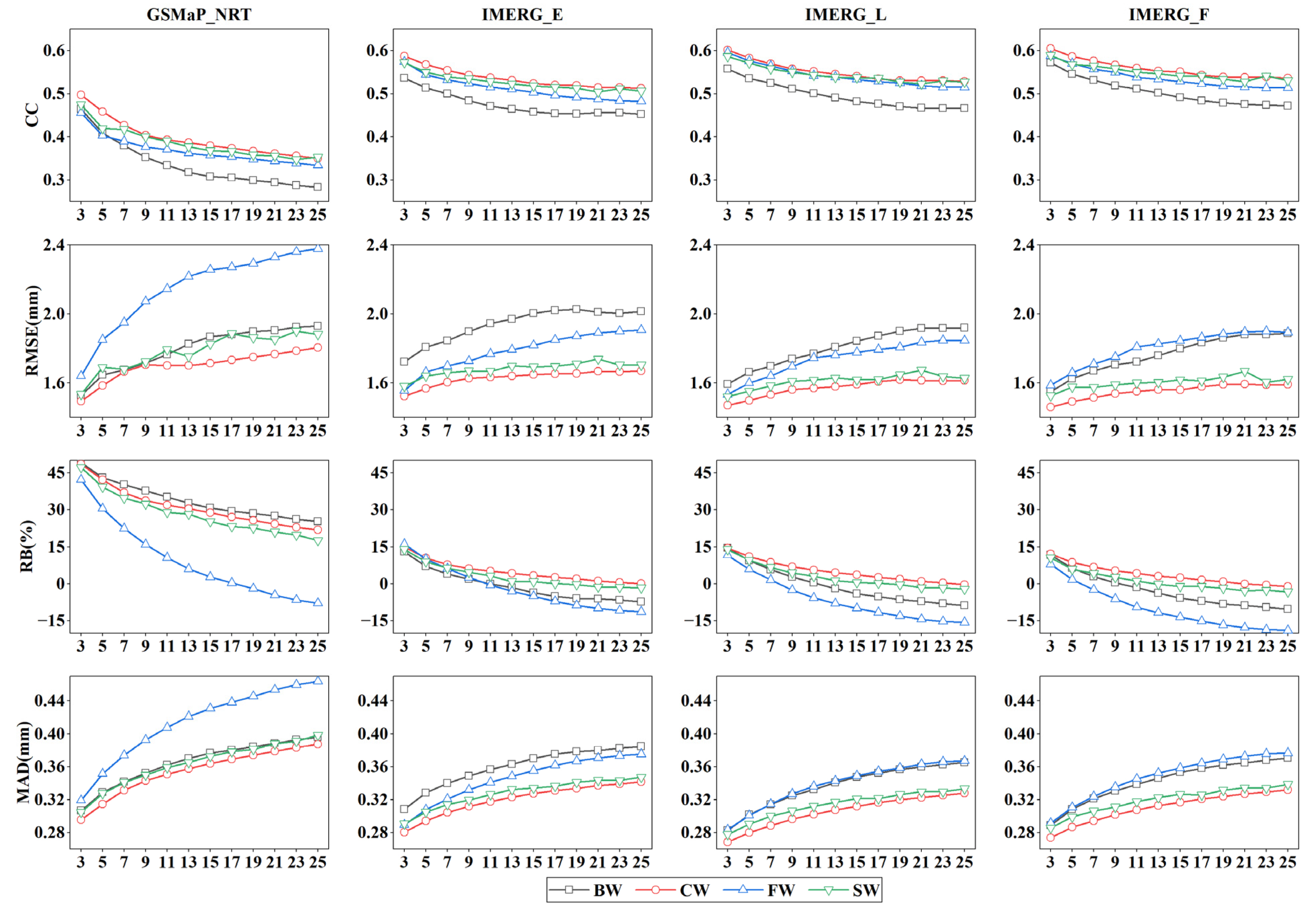
Four temporal windows (BW, CW, FW, and SW), ranging from 3 to 25 h, were used to correct the biases of the four hourly SPPs in the Shuaishui watershed. Figure 2 and Figure 3, respectively, compare the changes in the continuous and categorical evaluation metrics of the hourly SPPs after being corrected with the RBC using different temporal windows. As seen in Figure 2, the correlation coefficient (CC) values of all bias-corrected hourly SPPs tend to decrease with an increasing temporal window size before they gradually stabilize. Throughout the entire range of window sizes, the CC values of the SPPs corrected using CW consistently remain the highest, while those corrected using BW remain the lowest. Furthermore, the performances of the CW, FW, and SW are mostly similar.
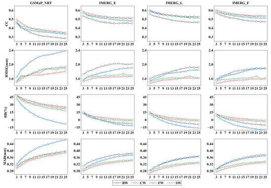
Figure 2.
Comparison of continuous evaluation metrics of the bias-corrected hourly satellite precipitation products during different temporal windows.
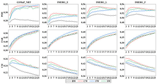
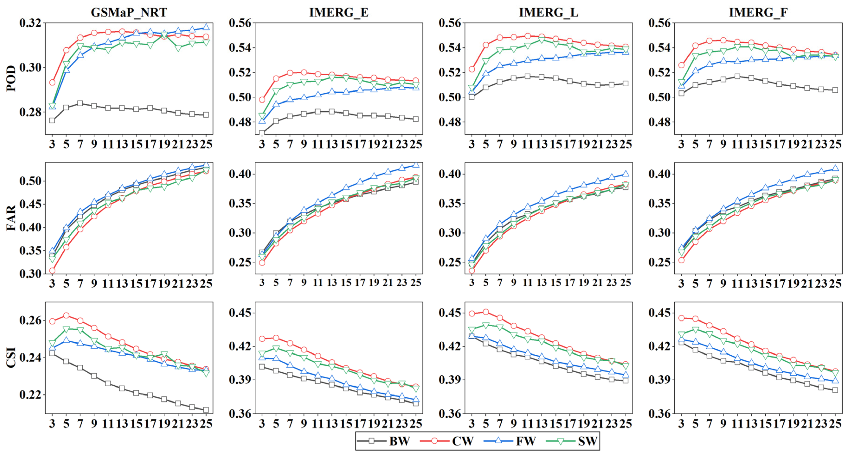
Figure 3.
Comparison of categorical evaluation metrics of the bias-corrected hourly satellite precipitation products during different temporal windows.
Unlike the CC, the root mean square error (RMSE) and mean absolute difference (MAD) of all bias-corrected SPPs tend to increase with the increasing window size before they eventually stabilize. Throughout the entire range of window sizes, the RMSE and MAD values of the bias-corrected SPPs using CW consistently remain the lowest. Meanwhile, FW performs the worst in terms of the RMSEs of GSMaP_NRT and IMERG_F, and the MADs of GSMaP_NRT, IMERG_L, and IMERG_F; BW performs the worst in terms of the RMSEs of IMERG_E and IMERG_L, and the MAD of IMERG_E. With regard to RB, FW performs the best in correcting GSMaP_NRT, while BW performs the worst. In addition, SW performs the best in correcting three IMERG products, while FW performs the worst (Figure 2).
As shown in Figure 3, the POD values of the four bias-corrected hourly SPPs all tend to increase with the window size when it falls between 3 and 7 h. However, the POD shows a slight fluctuation with further increase in the window size. Overall, CW performs the best while BW performs the worst in terms of the POD. Across the entire range of window sizes, the FAR values of all bias-corrected SPPs tend to increase with the window size. Four types of windows did not show much of a difference in terms of the FAR, with CW performing slightly better and FW slightly worse. Unlike the FAR, the CSIs of all bias-corrected SPPs tend to decrease with the window size, with CW performing better and BW performing worse (Figure 3).
After comparing the performances of the four types of windows in correcting all four hourly SPPs, the CW with a window size of 3 h was determined to be the optimal window for the RBC. The RBC correction results based on this window were used for a comparison with those of the PDF method.
3.2. Comparison of Performance in Correcting the Bias of Hourly Satellite Precipitation Products
3.2.1. Continuous Evaluation Metrics
Table 3 compares the continuous evaluation metrics of the hourly SPPs in the Shuaishui watershed before and after bias corrections. To date, there have been limited studies employing RBC and PDF for correcting the bias of hourly SPPs. Mastrantonas et al. (2019) found that their NRMSE values increased instead after they used the two methods to correct the bias of five hourly SPPs, including CMORPH, GSMaP, IMERG_E, IMERG_L, and PERSIANN [32]. Zhou et al. (2021) found that the RBC could barely improve the performance of hourly GSMaP-NRT and IMERG_E, while sometimes even causing an increase in the RMSE and MAE [49]. Unlike both studies, both RBC and PDF were able to improve the four SPPs to various degrees, as shown by a noticeable increase in the CC as well as reductions in both the RMSE and MAD. Furthermore, the PDF consistently performed better than the RBC in correcting the bias of all four hourly SPPs.
Table 3.
Comparison of the continuous evaluation metrics of the hourly satellite precipitation products before and after bias corrections in the Shuaishui watershed.
3.2.2. Categorical Evaluation Metrics
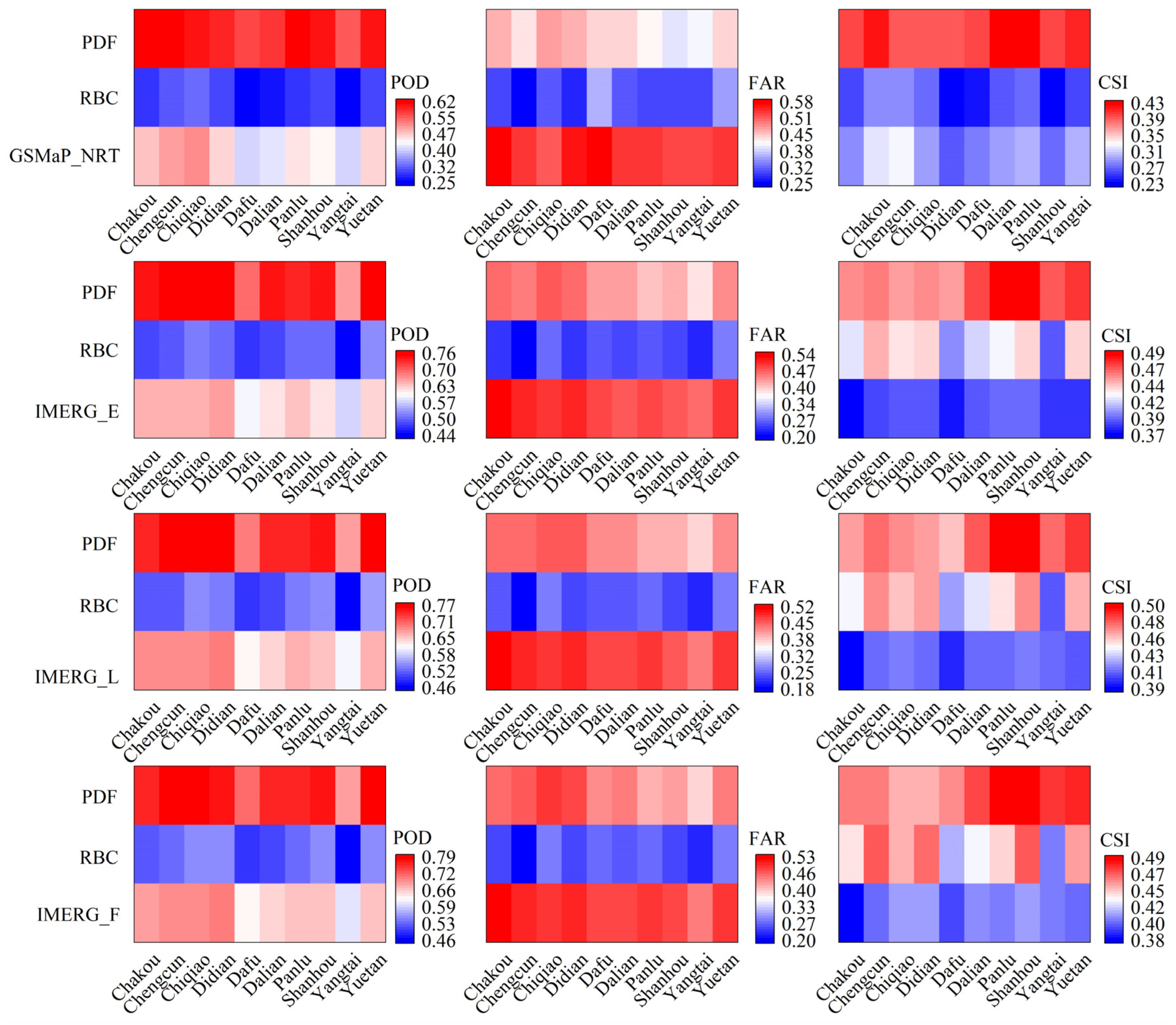
Figure 4 compares the changes in the three categorical evaluation metrics of the hourly SPPs before and after the bias corrections at ten rainfall stations in the Shuaishui watershed. The PDF could significantly improve the PODs of SPPs at all stations, while the RBC could barely improve the POD. Unlike the POD, both methods could improve the FARs of the four SPPs to varying degrees at all stations, with the RBC performing better than the PDF. Furthermore, both methods could improve the CSIs of the three IMERG products, with PDF performing better than RBC. For GSMaP_NRT, however, only PDF could improve its CSI.
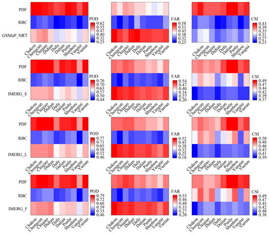
Figure 4.
Comparison of the categorical metrics of the hourly satellite precipitation products before and after bias corrections in the Shuaishui watershed.
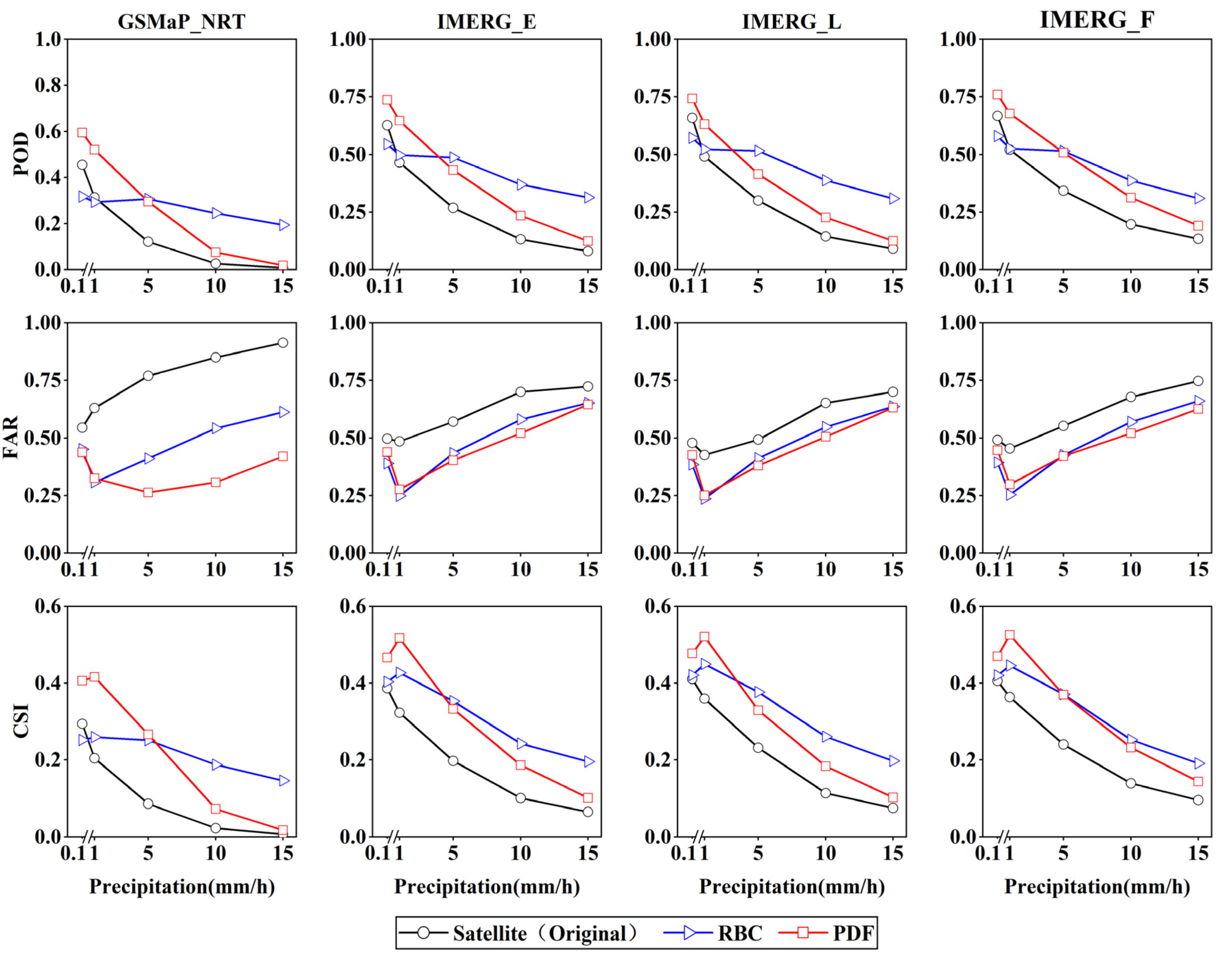
Figure 5 compares the efficacy of the four SPPs in detecting different hourly precipitation intensities before and after bias corrections. The POD of the SPPs decreases gradually with the increase in the hourly precipitation intensity, both before and after bias corrections. When the precipitation intensity is below 1 mm/h, the RBC does not improve the POD of the SPPs. However, when the intensity of precipitation exceeds 5 mm/h, the PODs of the four RBC-corrected products are higher than those of the PDF-corrected ones.
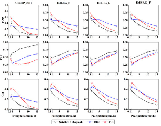
Figure 5.
Changes in the categorical metrics of the hourly satellite precipitation products with precipitation intensity before and after bias corrections.
As for the FAR, both bias correction methods initially resulted in a slight decrease in the FAR. With the further increase in hourly precipitation intensity, however, the FAR gradually increased. In general, the FARs of the three IMERG products were similar after RBC and PDF corrections. When the precipitation intensity was above 5 mm/h, the FARs of the four PDF-corrected products was better than those of the RBC-corrected products.
The CSIs of all bias-corrected SPPs increased slightly with increasing hourly precipitation intensities when they were less than 1 mm/h. Then, however, the CSIs of the bias-corrected SPPs gradually decreased with the increase in the precipitation intensity. For the three IMERG products, the PDF performed better than the RBC when the precipitation intensity was less than 1 mm/h, but showed the opposite when the precipitation intensity was above 5 mm/h. For GSMaP_NRT, PDF performed slightly better when the precipitation intensity was less than 5 mm/h, while RBC performed better when the precipitation intensity was above 10 mm/h.
3.3. Hydrological Simulation Evaluation of the Hourly Satellite Precipitation Products
3.3.1. Hydrological Parameter Calibration of the SWAT Models
SWAT-CUP 2019 is a software specifically designed for calibrating the parameters of SWAT models. Integrating model calibration, uncertainty analysis, and parameter sensitivity analysis, SWAT-CUP has advantages, such as a high computational efficiency and visualization of calibration results [50].
Ground rainfall observations, four original SPPs (GSMaP_NRT, IMERG_E, IMERG_L, and IMERG_F), and eight bias-corrected SPPs were separately used as the rainfall inputs to SWAT. The hydrological parameters of these SWAT models were calibrated and validated separately, whose calibration and validation periods all spanned from 2010 to 2013 and from 2014 to 2017, respectively. In each SWAT model, fifteen SWAT hydrological parameters were calibrated using the SUFI-2 algorithm of SWAT-CUP [51]. Table 4 shows the hydrological parameter calibration results of the SWAT models.
Table 4.
Results of SWAT hydrological parameter calibration.
3.3.2. Comparison of the Hydrological Simulation Results Based on the Hourly Precipitation
Table 5 compares the hydrological simulation performances of different SWAT models at the Yuetan Hydrological Station during both calibration and validation stages. The SWAT model driven by the hourly precipitation data from ground rain stations shows a very good performance in simulating the daily streamflow during both calibration and validation stages, with NSEs of 0.91 and 0.91, R2 values of 0.92 and 0.91, and RBs of −9.36% and −7.79%, respectively. Among the four SWAT models driven by the original hourly SPPs, the model based on IMERG_F performed the best, with NSEs of 0.77 and 0.75, R2 values of 0.78 and 0.78, and RBs of −23.88% and −21.94% during calibration and validation, respectively. Meanwhile, the model based on GSMaP_NRT performed the worst, with NSEs of 0.30 and 0.26, R2 values of 0.34 and 0.34, and RBs of −18.20% and −17.53% during calibration and validation, respectively.
Table 5.
Comparison of the simulation performance among the SWAT models with different rainfall inputs in the Shuaishui watershed.
In comparison to those based on the original hourly SPPs, the hydrological simulation performance of the SWAT models based on the bias-corrected SPPs improved considerably with a large increase in both R2 and NSE and a decrease in absolute RB values. For example, the NSE and R2 of the SWAT model based on the PDF-corrected GSMaP_NRT increased considerably to 0.70 and 0.77 during calibration, and 0.69 and 0.55 during validation, respectively. Except for IMERG_E, the SWAT models utilizing the PDF-corrected SPPs were superior to the corresponding models utilizing the RBC-corrected SPPs. Among the four SPPs corrected with PDF, the SWAT model based on the PDF-corrected IMERG_F performed the best with an NSE and R2 of 0.82 and 0.84 during calibration, and 0.81 and 0.86 during validation, respectively.
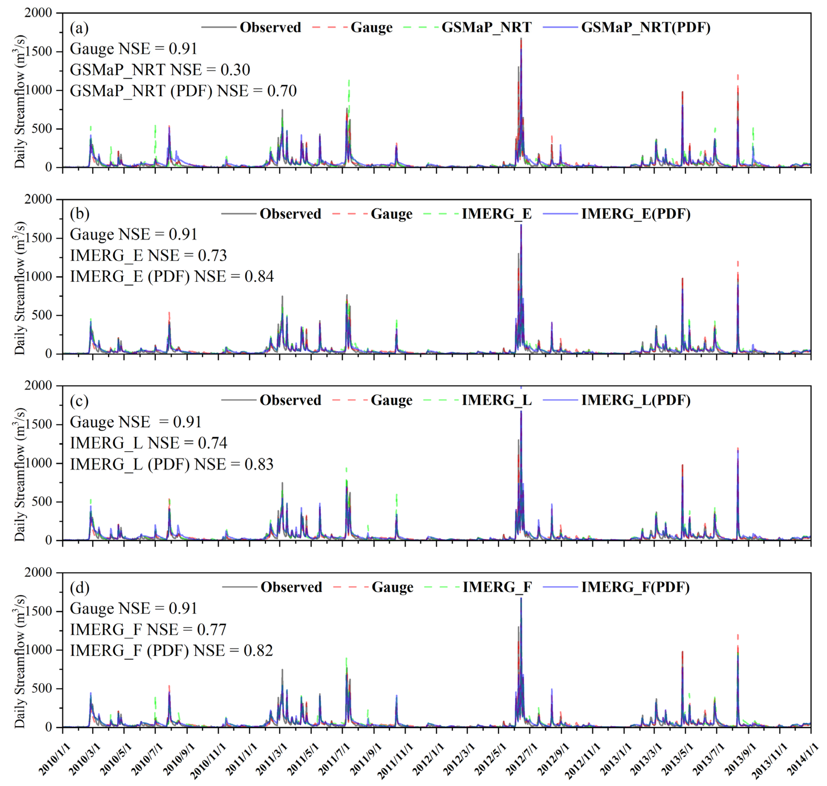
Figure 6 and Figure 7, respectively, compare the simulated daily streamflow at the Yuetan station among the SWAT models during the calibration and validation periods, which are respectively driven by ground rainfall observations, original SPPs, and PDF-corrected SPPs. As seen from the figures, SWAT models based on different hourly precipitation inputs are all able to capture the general trend of the observed daily streamflow. Regardless of being corrected by the PDF or not, the simulated streamflow by the SWAT models driven by the hourly SPPs could closely match the observed streamflow during the dry season (November to the following March). During the wet season (April to October), however, there is much discrepancy in the simulated levels of streamflow by different SWAT models. Specifically, on the days with a high daily streamflow, the SWAT models driven by PDF-corrected SPPs tend to simulate the streamflow better than those driven by original SPPs. During the calibration period, for example, the observed daily streamflow on 14 July 2011 was 259.00 m3/s; the simulated streamflow by the SWAT model utilizing ground rainfall was 254.40 m3/s, compared to the excessive amount of 1129.00 m3/s given by the SWAT model utilizing GSMaP_NRT and 211.90 m3/s by the model utilizing the PDF-corrected GSMaP_NRT (Figure 6a). On 11 August 2013, the observed streamflow was 968.00 m3/s, while the simulated streamflow values by the SWAT model using ground rainfall, IMERG_E, and PDF-corrected IMERG_E were 1199.00 m3/s, 373.40 m3/s, and 890.70 m3/s, respectively (Figure 6b). On 11 July 2011, the observed streamflow was 379.00 m3/s, while the simulated streamflow values by the SWAT model using ground rainfall observations, IMERG_L, and PDF-corrected IMERG_L were 376.10 m3/s, 635.40 m3/s, and 402.90 m3/s, respectively (Figure 6c). On 25 April 2013, the observed streamflow was 979.00 m3/s, while the simulated streamflow values by the SWAT model using ground rainfall observation, IMERG_F, and PDF-corrected IMERG_F were 1004.00 m3/s, 561.20 m3/s, and 765.80 m3/s, respectively (Figure 6d).
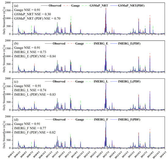
Figure 6.
Comparison between observed and simulated daily streamflows at the Yuetan Hydrological Station during the calibration period by the SWAT models using ground rainfall observations, original satellite precipitation products, and PDF-corrected satellite precipitation products: (a) GSMaP_NRT; (b) IMERG_E; (c) IMERG_L; (d) IMERG_F.
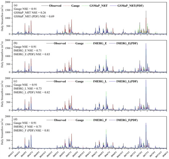
Figure 7.
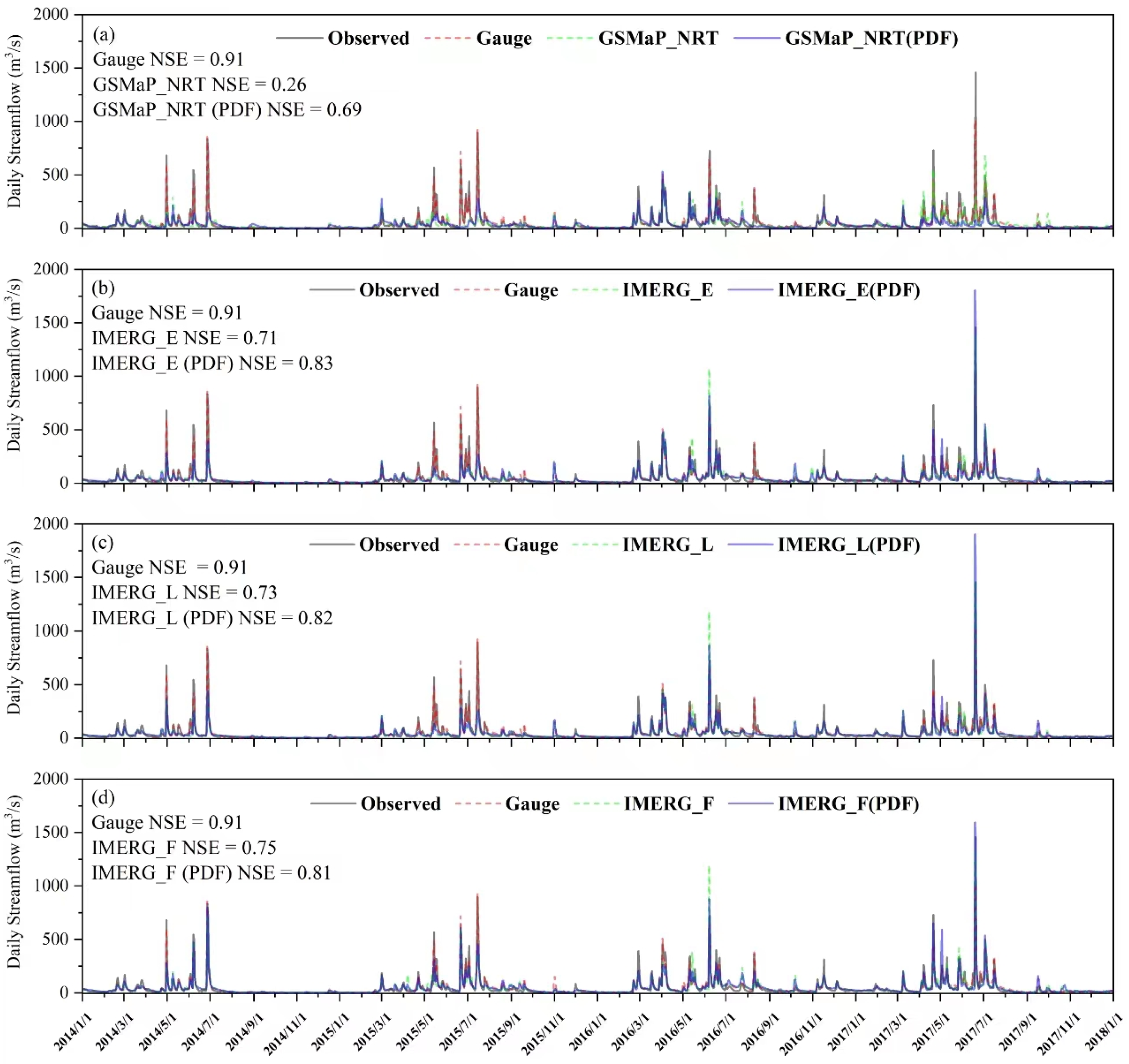
Comparison between observed and simulated daily streamflows at the Yuetan Hydrological Station during the validation period by the SWAT models using ground rainfall observations, original satellite precipitation products, and PDF-corrected satellite precipitation products: (a) GSMaP_NRT; (b) IMERG_E; (c) IMERG_L; (d) IMERG_F.
Similarly, during the validation period, the observed daily streamflow on 4 July 2017 was 419.00 m3/s; the simulated streamflow by the SWAT model utilizing ground rainfall was 380.80 m3/s, compared to 925.40 m3/s by the SWAT model utilizing GSMaP_NRT and 367.20 m3/s by the model utilizing the PDF-corrected GSMaP_NRT (Figure 7a). On 7 June 2016, the observed streamflow was 649.00 m3/s, while the simulated streamflow values by the SWAT model using ground rainfall, IMERG_E, and PDF-corrected IMERG_E were 591.10 m3/s, 1073.00 m3/s, and 818.20 m3/s, respectively (Figure 7b). On 20 June 2017, the observed streamflow is 1460.00 m3/s, while the simulated streamflow values by the SWAT model using ground rainfall observations, IMERG_L, and PDF-corrected IMERG_L were 1182.00 m3/s, 2038.00 m3/s, and 1453.00 m3/s, respectively (Figure 7c). On 21 April 2017, the observed streamflow was 733.00 m3/s, while the simulated streamflow values by the SWAT model using ground rainfall observation, IMERG_F, and PDF-corrected IMERG_F were 458.40 m3/s, 313.50 m3/s, and 654.70 m3/s, respectively (Figure 7d). It is evident that the hydrological simulation performance of SWAT is significantly improved after the original hourly SPPs are replaced with the PDF-corrected counterparts. The simulated streamflow by the SWAT models utilizing the bias-corrected hourly SPPs could closely match the observed streamflow, and in some cases, was even better than that simulated by the SWAT model based on ground rainfall observations. Therefore, the product could be applied for streamflow simulations and predictions in areas with sparse ground rainfall stations.
4. Conclusions
In this study, four hourly satellite precipitation products (GSMaP_NRT, IMERG_E, IMERG_L, and IMERG) were bias-corrected with two methods, namely, RBC and PDF, in the Shuaishui watershed, which were then used as rainfall inputs for the SWAT models to assess their applicability in hydrological simulation studies.
(1) Both RBC and PDF could improve the accuracy of the four hourly satellite precipitation products to various degrees. In general, PDF performed better than RBC in the bias correction. After being corrected with the PDF, all four SPPs had CC values above 0.65 and absolute RB values less than 37%. The rainfall detection capability of the four PDF-corrected SPPs in terms of the CSI also improved considerably.
(2) The SWAT models utilizing the PDF-corrected hourly SPPs could simulate the daily streamflow at Yuetan station in the Shuaishui watershed better than those utilizing the RBC-corrected SPPs, whose NSE values surpassed 0.75 during both the calibration and validation periods. Among the bias-corrected SPPs, PDF-corrected IMERG_F performed the best with an R2 of 0.84, NSE of 0.82, and RB of −18.56% during calibration, and an R2 of 0.86, NSE of 0.81, and RB of −17.05% during validation. After being bias-corrected, the hourly satellite precipitation product could be applied well to simulate the daily streamflow in the region.
(3) As a research hotspot in the field of artificial intelligence, machine learning has been increasingly widely applied to solve complex problems in various engineering and scientific fields. In the future, the usage of different machine learning methods, such as random forest and neural networks, can be explored to correct the bias of hourly satellite precipitation products.
Author Contributions
Conceptualization, J.Y. and X.Y.; data curation, Y.L. and J.Y.; formal analysis, Y.L., J.Y. and X.Y.; funding acquisition, X.Y.; investigation, J.Y., Y.L. and Z.H.; methodology, X.Y. and J.Y.; project administration, X.Y., J.Y. and Y.L.; resources, J.Y. and Y.L.; software, Y.L. and X.Y.; supervision, X.Y.; validation, J.Y., X.Y. and Z.H.; visualization, Y.L. and X.Z.; writing—original draft preparation, J.Y. and Y.L.; writing—review and editing, J.Y., Y.L., X.Y., Z.H., P.H. and X.Z. All authors have read and agreed to the published version of the manuscript.
Funding
This study was supported by the National Key Research and Development Program of China (Grant, 2023YFC3708800), the Belt and Road Special Foundation of the State Key Laboratory of Hydrology—Water Resources and Hydraulic Engineering at Nanjing Hydraulic Research Institute, China (Grant, 2018nkzd01), and the Natural Science Fund of Anhui Province of China (Grant, 2308085MD127).
Data Availability Statement
The SWAT model can be downloaded from https://swat.tamu.edu/. The meteorological data is provided by the Tunxi Meteorological Station in Huangshan City. The satellite precipitation products are available at https://pmm.nasa.gov/.
Conflicts of Interest
The authors declare no conflict of interest.
References
- Wu, P.L.; Christidis, N.; Stott, P. Anthropogenic impact on earth’s hydrological cycle. Nat. Clim. Change 2013, 3, 807–810. [Google Scholar] [CrossRef]
- Allen, M.R.; Ingram, W.J. Constraints on future changes in climate and the hydrologic cycle. Nature 2012, 489, 590. [Google Scholar] [CrossRef]
- Wang, S.; Zhang, L.; Yu, X.; She, D.; Gan, Y. Application of remote sensing precipitation products in runoff simulation over the Lancang River Basin. Resour. Environ. Yangtze Basin 2019, 28, 1365–1374. [Google Scholar]
- Tan, M.L.; Samat, N.; Chan, N.W.; Roy, R. Hydro-Meteorological assessment of three GPM satellite precipitation products in the Kelantan River Basin, Malaysia. Remote Sens. 2018, 10, 1011. [Google Scholar] [CrossRef]
- Darand, M.; Siavashi, Z. An evaluation of Global Satellite Mapping of Precipitation (GSMaP) datasets over Iran. Meteorol. Atmos. Phys. 2021, 133, 911–923. [Google Scholar] [CrossRef]
- Hao, Z.; Tong, K.; Zhang, L.; Duan, X. Applicability analysis of TRMM precipitation estimates in Tibetan plateau. Hydrology 2011, 31, 18–23. [Google Scholar]
- Li, X.; Chen, S.; Liang, Z.; Huang, C.; Li, Z.; Hu, B. Performance assessment of GSMaP and GPM IMERG products during Typhoon Mangkhut. Atmosphere 2021, 12, 134. [Google Scholar] [CrossRef]
- Palomino-Angel, S.; Anaya-Acevedo, J.A.; Botero, B.A. Evaluation of 3B42V7 and IMERG daily-precipitation products for a very high-precipitation region in northwestern South America. Atmos. Res. 2019, 217, 37–48. [Google Scholar] [CrossRef]
- Prakash, S. Performance assessment of CHIRPS, MSWEP, SM2RAIN-CCI, and TMPA precipitation products across India. J. Hydrol. 2019, 571, 50–59. [Google Scholar] [CrossRef]
- Serrat-Capdevila, A.; Merino, M.; Valdes, J.B.; Durcik, M. Evaluation of theperformance of three satellite precipitation products over Africa. Remote Sens. 2016, 8, 836. [Google Scholar] [CrossRef]
- Mou Leong, T.; Santo, H. Comparison of GPM IMERG, TMPA 3B42 and PERSIANN-CDR satellite precipitation products over Malaysia. Atmos. Res. 2018, 202, 63–76. [Google Scholar]
- Navarro, A.; Garcia-Ortega, E.; Merino, A.; Luis Sanchez, J.; Tapiador, F.J. Orographic biases in IMERG precipitation estimates in the Ebro River Basin (Spain): The effects of rain gauge density and altitude. Atmos. Res 2020, 244, 105068. [Google Scholar] [CrossRef]
- Sorooshian, S.; AghaKouchak, A.; Arkin, P.; Eylander, J.; Foufoula-Georgiou, E.; Harmon, R.; Hendrickx, J.M.H.; Imam, B.; Kuligowski, R.; Skahill, B.; et al. Advanced concepts on remote sensing of precipitation at multiple scales. Bull. Am. Meteorol. Soc. 2011, 92, 1353–1357. [Google Scholar] [CrossRef]
- Yu, L.; Ma, L.; Li, H.; Zhang, Y.; Kong, F.; Yang, Y. Assessment of high-resolution satellite rainfall products over a gradually elevating mountainous terrain based on a high-density rain gauge network. Int. J. Remote Sens. 2020, 41, 5620–5644. [Google Scholar] [CrossRef]
- Li, N.; Tang, G.; Zhao, P.; Hong, Y.; Gou, Y.; Yang, K. Statistical assessment and hydrological utility of the latest multi-satellite precipitation analysis IMERG in Ganjiang River Basin. Atmos. Res. 2017, 183, 212–223. [Google Scholar] [CrossRef]
- Li, Q.; Wei, J.; Yin, J.; Qiao, Z.; Peng, W.; Peng, H. Multiscale Comparative evaluation of the GPM and TRMM precipitation products against ground precipitation observations over Chinese Tibetan Plateau. IEEE J. Sel. Top. Appl. Earth Obs. Remote Sens. 2021, 14, 2295–2313. [Google Scholar] [CrossRef]
- Xu, S.; Shen, Y.; Niu, Z. Evaluation of the IMERG version 05B precipitation product and comparison with IMERG version 04A over mainland China at hourly and daily scales. Adv. Space Res. 2019, 63, 2387–2398. [Google Scholar] [CrossRef]
- Yang, X.; Lu, Y.; Tan, M.L.; Li, X.; Wang, G.; He, R. Nine-year systematic evaluation of the GPM and TRMM precipitation products in the Shuaishui River Basin in East-central China. Remote Sens. 2020, 12, 1042. [Google Scholar] [CrossRef]
- Yuan, F.; Zhang, L.; Soe, K.M.W.; Ren, L.; Zhao, C.; Zhu, Y.; Jiang, S.; Liu, Y. Applications of TRMM- and GPM-Era multiple-satellite precipitation products for flood simulations at sub-daily scales in a sparsely gauged watershed in Myanmar. Remote Sens. 2019, 11, 140. [Google Scholar] [CrossRef]
- Lewis, E.; Quinn, N.; Blenkinsop, S.; Fowler, H.J.; Freer, J.; Tanguy, M.; Hitt, O.; Coxon, G.; Bates, P.; Woods, R. A rule based quality control method for hourly rainfall data and a 1 km resolution gridded hourly rainfall dataset for Great Britain: CEH-GEAR1hr. J. Hydrol. 2018, 564, 930–943. [Google Scholar] [CrossRef]
- Meaurio, M.; Zabaleta, A.; Srinivasan, R.; Sauvage, S.; Sanchez-Perez, J.-M.; Lechuga-Crespo, J.L.; Antiguedad, I. Long-term and event-scale sub-daily streamflow and sediment simulation in a small forested catchment. Hydrol. Sci. J. 2021, 66, 862–873. [Google Scholar] [CrossRef]
- Bastola, S.; Misra, V. Sensitivity of hydrological simulations of southeastern United States watersheds to temporal aggregation of rainfall. J. Hydrometeorol. 2013, 14, 1334–1344. [Google Scholar] [CrossRef]
- Li, X.; Huang, S.; He, R.; Wang, G.; Tan, M.L.; Yang, X.; Zheng, Z. Impact of temporal rainfall resolution on daily streamflow simulations in a large-sized river basin. Hydrol. Sci. J. 2020, 65, 2630–2645. [Google Scholar] [CrossRef]
- Cheema, M.J.M.; Bastiaanssen, W.G.M. Local calibration of remotely sensed rainfall from the TRMM satellite for different periods and spatial scales in the Indus Basin. Int. J. Remote Sens. 2012, 33, 2603–2627. [Google Scholar] [CrossRef]
- Manz, B.; Buytaert, W.; Zulkafli, Z.; Lavado, W.; Willems, B.; Alberto Robles, L.; Rodriguez-Sanchez, J.-P. High-resolution satellite-gauge merged precipitation climatologies of the Tropical Andes. J. Geophys. Res. Atmos. 2016, 121, 1190–1207. [Google Scholar] [CrossRef]
- Krajewski, W.F. Cokriging radar-rainfall and rain-gauge data. J. Geophys. Res. Atmos. 1987, 92, 9571–9580. [Google Scholar] [CrossRef]
- Rosenfeld, D. The window probability matching method for rainfall measurements with radar-reply. J. Appl. Meteorol. 1997, 36, 247–249. [Google Scholar] [CrossRef]
- Todini, E. A Bayesian technique for conditioning radar precipitation estimates to rain-gauge measurements. Hydrol. Earth Syst. Sci. 2001, 5, 187–199. [Google Scholar] [CrossRef]
- Shen, Y.; Zhao, P.; Pan, Y.; Yu, J. A high spatiotemporal gauge-satellite merged precipitation analysis over China. J. Geophys. Res. Atmos. 2014, 119, 3063–3075. [Google Scholar] [CrossRef]
- Liu, X.; Yong, Z.; Liu, L.; Chen, T.; Zhou, L.; Li, J. Improving hydrological simulation accuracy through a three-step bias correction method for satellite precipitation products with limited gauge data. Water 2023, 15, 3615. [Google Scholar] [CrossRef]
- Ziarh, G.F.; Shahid, S.; Bin Ismail, T.; Asaduzzaman, M.; Dewan, A. Correcting bias of satellite rainfall data using physical empirical model. Atmos. Res. 2021, 251, 105430. [Google Scholar] [CrossRef]
- Mastrantonas, N.; Bhattacharya, B.; Shibuo, Y.; Rasmy, M.; Espinoza-Davalos, G.; Solomatine, D. Evaluating the benefits of merging near-real-time satellite precipitation products: A case study in the Kinu Basin region, Japan. J. Hydrometeorol. 2019, 20, 1213–1233. [Google Scholar] [CrossRef]
- Deng, P.; Zhang, M.; Bing, J.; Jia, J.; Zhang, D. Evaluation of the GSMaP_Gauge products using rain gauge observations and SWAT model in the upper Hanjiang River Basin. Atmos. Res. 2019, 219, 153–165. [Google Scholar] [CrossRef]
- Kha Dang, D.; Tran Ngoc, A.; Nguyen, N.Y.; Du Duong, B.; Srinivasan, R. Evaluation of grid-based rainfall products and water balances over the Mekong River Basin. Remote Sens. 2020, 12, 1858. [Google Scholar]
- Setti, S.; Maheswaran, R.; Sridhar, V.; Barik, K.K.; Merz, B.; Agarwal, A. Inter-comparison of gauge-based gridded data, reanalysis and satellite precipitation product with an emphasis on hydrological modeling. Atmosphere 2020, 11, 1252. [Google Scholar] [CrossRef]
- Wang, X.; Li, B.; Chen, Y.; Guo, H.; Wang, Y.; Lian, L. Applicability evaluation of multisource satellite precipitation data for hydrological research in arid mountainous areas. Remote Sens. 2020, 12, 2886. [Google Scholar] [CrossRef]
- Mo, C.; Zhang, M.; Ruan, Y.; Qin, J.; Wang, Y.; Sun, G.; Xing, Z. Accuracy analysis of IMERG satellite rainfall data and its application in long-term runoff simulation. Water 2020, 12, 2177. [Google Scholar] [CrossRef]
- Lu, Y.; Tu, J.; Gao, Z.; Li, X.; Yang, S.; Yang, X. Impact of temporal rainfall resolution on SWAT hydrological simulation. China Environ. Sci. 2020, 40, 5383–5390. [Google Scholar]
- Huang, S.; Lu, Y.; Yang, X.; Li, X. Study on spatio-temporal trends of the green development of Huangshan city in Anhui province. Resour. Environ. Yangtze Basin 2019, 28, 1872–1885. [Google Scholar]
- Kubota, T.; Aonashi, K.; Ushio, T.; Shige, S.; Takayabu, Y.N.; Kachi, M.; Arai, Y.; Tashima, T.; Masaki, T.; Kawamoto, N. Global Satellite Mapping of Precipitation (GSMaP) products in the GPM era. In Satellite Precipitation Measurement; Springer: Cham, Switzerland, 2020; Volume 1, pp. 355–373. [Google Scholar]
- Liu, J.; Sun, Z.; Zhang, T.; Cheng, X.; Dong, X.; Tan, X. Hydrological evaluations of runoff simulations based on multiple satellite precipitation products over the Huayuan Catchment. Resour. Environ. Yangtze Basin 2018, 27, 2558–2567. [Google Scholar]
- Habib, E.; Haile, A.T.; Sazib, N.; Zhang, Y.; Rientjes, T. Effect of bias correction of satellite-rainfall estimates on runoff simulations at the source of the upper Blue Nile. Remote Sens. 2014, 6, 6688–6708. [Google Scholar] [CrossRef]
- Ines, A.V.M.; Hansen, J.W. Bias correction of daily GCM rainfall for crop simulation studies. Agric. For. Meteorol. 2006, 138, 44–53. [Google Scholar] [CrossRef]
- Song, W.; Xie, X.; Xu, T.; Wang, C.; Zhou, D. Construction of hydrological processes model and analysis of hydrological functions of marsh wetlands in Honghe region. Wetl. Sci. 2014, 12, 544–551. [Google Scholar]
- Liu, J.; Wei, R.; Zhang, T.; Zhang, Q.; Liu, Y. Spatial and temporal evolution characteristics of dry and wet condition in Yalongjiang River Basin based on the CHIRPS satellite precipitation. Resour. Environ. Yangtze Basin 2020, 29, 1800–1811. [Google Scholar]
- Cui, L.; Wang, S.; Liu, Y.; Jiang, Y.; Dong, L.; Huang, C. Comparative study on downscaling of TRMM and GPM satellite precipitation data in three major river basins in China. Resour. Environ. Yangtze Basin 2021, 30, 1317–1328. [Google Scholar]
- Jiang, S.; Ren, L.; Yong, B.; Yuan, F.; Gong, L.; Yang, X. Hydrological evaluation of the TRMM multi-satellite precipitation estimates over the Mishui Basin. Adv. Water Sci. 2014, 25, 641–649. [Google Scholar]
- Zhang, S.; Yu, P.; Wang, Y.; Zhang, H.; Valentina, K.; Huang, S.; Xiong, W.; Xu, L. Estimation of actual evapotranspiration and its component in the upstream of Jinghe Basin. Acta Geogr. Sin. 2011, 66, 385–395. [Google Scholar]
- Zhou, L.; Rasmy, M.; Takeuchi, K.; Koike, T.; Selvarajah, H.; Ao, T. Adequacy of near real-time satellite precipitation products in driving flood discharge simulation in the Fuji River Basin, Japan. Appl. Sci. 2021, 11, 1087. [Google Scholar] [CrossRef]
- Abbaspour, K.C.; Vejdani, M.; Haghighat, S. SWAT-CUP calibration and uncertainty programs for SWAT. In Proceedings of the International Congress on Modelling and Simulation (MODSIM07), Christchurch, New Zealand, 10–13 December 2007. [Google Scholar]
- Patii, M.; Kothari, M.; Gorantiwar, S.D. Runoff simulation using the SWAT model and SUFI-2 algorithm in Ghod Catchment of upper Bhima River Basin. Indian J. Soil Conserv. 2019, 47, 7–13. [Google Scholar]
Disclaimer/Publisher’s Note: The statements, opinions and data contained in all publications are solely those of the individual author(s) and contributor(s) and not of MDPI and/or the editor(s). MDPI and/or the editor(s) disclaim responsibility for any injury to people or property resulting from any ideas, methods, instructions or products referred to in the content. |
© 2023 by the authors. Licensee MDPI, Basel, Switzerland. This article is an open access article distributed under the terms and conditions of the Creative Commons Attribution (CC BY) license (https://creativecommons.org/licenses/by/4.0/).