Abstract
The distributed Grid-Xin’anjiang (Grid-XAJ) model is very sensitive to the spatial and temporal distribution of data when used in humid and semi-humid small and medium catchments. We used the successive correction method to merge the gauged rainfall with rainfall forecasted by the Weather Research and Forecasting (WRF) model to enhance the spatiotemporal accuracy of rainfall distribution. And we used the Penman–Monteith equation to calculate the potential evapotranspiration (PEPM). Then, we designed two forcing scenarios (WRF-driven rainfall (Wr) + PEPM, WRF-merged rainfall (Wm) + PEPM) to drive the Grid-XAJ model for flood forecasting. We found the WRF-driven Grid-XAJ model held significant potential in flood forecasting. The Grid-XAJ model provided only an approximation of flood hygrographs when driven by scenario Wr + PEPM. The results in scenario Wm + PEPM showed a high degree-of-fit with observed floods with mean Nash–Sutcliffe efficiency coefficient (NSE) values of 0.94 and 0.68 in two catchments. Additionally, scenario Wm + PEPM performed better flood hygrographs than scenario Wr + PEPM. The flood volumes and flow peaks in scenario Wm + PEPM had an obvious improvement compare to scenario Wr + PEPM. Finally, we observed that the model exhibited superior performance in forecasting flood hydrographs, flow peaks, and flood volumes in humid catchments compared with semi-humid catchments.
1. Introduction
Floods are one of the most serious natural disasters, and in recent years, they have received increasing attention [1,2]. The primary economic and demographic focal points of China are primarily concentrated in humid and semi-humid regions, thus emphasizing the paramount significance of studying flood forecasting in these areas [3]. In recent years, the risk of extreme floods in the large basins of China has been substantially reduced due to improvements in flood forecasting [4]. However, the floods that occur in small and medium catchments (SMCs) are characterized by rapidity and suddenness, and usually have a short flood duration and cause a rapid rise in the flow peak, which makes flood prediction difficult [5]. Moreover, flood forecasting in both humid SMCs and semi-humid SMCs faces additional challenges due to the fact that flood forecasting in SMCs is more sensitive to the spatial and temporal distribution of data.
Hydrological models serve as important tools in flood forecasting and have been widely used in various regions [5,6]. Hydrological models can be classified into lumped, semi-distributed, and distributed models on the basis of the hydrological processes and watershed attributes [7,8,9]. In this study, we used the Grid-XAJ model [10] for flood forecasting. It is a distributed version of the well-known Xin’anjiang model. This model has been widely used in numerous catchments throughout China [11,12]. It operates at a high resolution (≤1 km) and conducts flood calculations for each grid cell, thereby incorporating the spatial variability of rainfall and the underlying surface conditions more effectively. Traditionally, the Grid-XAJ model is driven by gauged rainfall and pan evaporations [10], which overlook the comprehensive influence of meteorology on hydrological processes. Additionally, distributed hydrological models require grid data driving [13]. The grid data for the Grid-XAJ model are usually generated using spatial interpolation methods. The accuracy of station observations is relatively high, and the uncertainty in expressing the characteristics of a meteorological element at the basin scale using station observations is largely due to interpolation or data assimilation processes.
The precise calibration of parameters in the hydrological model is crucial for accurately simulating floods [14,15]. Some parameters of the Grid-XAJ model can be a priori estimated using underlying surface data. For instance, the channel bed slope (Soc) can be estimated utilizing the digital elevation model (DEM), and the leaf area index (LAI) can be estimated based on land use and land cover (LULC) data. On the other hand, other parameters necessitate calibration. Over time, the Grid-XAJ model has undergone continuous development and refinement.
Acquiring reliable rainfall spatial information on high temporal resolution is essential to improve the ability of flood forecasting for the Grid-XAJ model. Typically, researchers interpolate gauged rainfall onto computational units to drive the Grid-XAJ model [16]. However, rainfall spatial interpolation is a non-trivial task due to many challenging factors, such as the rainfall’s irregular distribution in space, and the accuracy of the interpolation results is sometimes unsatisfactory [17,18]. Several methods have been employed to improve the interpolation results, such as graph neural networks (GNNs) [19,20] and graph for spatial interpolation (GSI) [21]. Additionally, various numerical weather prediction (NWM) models are used to achieve high spatial resolution in rainfall data [22]. For example, the Weather Research and Forecasting (WRF) model has a proven potential in depicting the spatial distribution of rainfall [23]. It has been used by Yao [24] to generate rainfall data for the Grid-XAJ model. However, WRF-driven rainfall often underestimates both the rain area and its intensity [25,26]. To enhance the reliability of rainfall predictions, a range of methods have been employed to merge WRF rainfall with multiple sources [27]. In this study, we used a successive correction method [28] to merge the WRF-driven rainfall with gauged rainfall to improve the spatio-temporal accuracy of rainfall distribution.
Pan evaporation is another type of input gauged data for the Grid-XAJ model, which is converted into potential evapotranspiration (PE) using the pan coefficient (KC). Evapotranspiration (ET) plays a crucial role in facilitating water–energy exchange between the land surface and atmosphere [29,30,31]. The accurate assessment of PE is significant for studying hydrological cycle processes and achieving full coupling between hydrological models and meteorological models. The hourly PE in the Grid-XAJ model is calculated for each grid by evenly distributing the daily pan evaporation across each hour (PEpan). However, usually only one or two pans are available within a catchment, and these pans exclusively capture daily evaporation. So the PEpan may not resonate with real-world conditions [32,33]. Various methods can improve the spatiotemporal accuracy of PE distribution. With the advancement of remote sensing technology, a growing number of datasets now directly offer high-spatial-resolution PE data with reliable accuracy at no cost. Notable examples include the Moderate Resolution Imaging Spectroradiometer (MODIS) [34] and the Global Land Evaporation Amsterdam Model (GLEAM) [35]. But their temporal resolution is sometimes not satisfactory. Acquiring high-spatiotemporal-resolution meteorological variables such as temperature and wind speed is considerably easy. Hence, machine learning methods with the inputs of meteorological data have been extensively employed for the best PE estimates in recent years [36,37]. In addition, using energy-based methods to estimate PE with high-spatiotemporal-resolution meteorological data is reliable. For example, the Penman–Monteith equation, which is based on energy balance, has been used by Meng [38] to effectively estimate the temporal and spatial distribution of PE in the Grid-XAJ model. We employed the Penman–Monteith equation to evaluate the potential evapotranspiration (PEPM) using meteorological data generated by the WRF model in this paper.
The objective of this study is to enhance the accuracy of the spatial and temporal distribution of rainfall and PE in the Grid-XAJ model via the utilization of the WRF model. This enhancement aims to improve the flood simulations of the Grid-XAJ model. To accomplish this objective, we initially compared three rainfall products based on WRF-driven rainfall and gauged rainfall. Then, we analyzed the characteristics of PEPM. Finally, to comprehensively assess the WRF-driven Grid-XAJ model’s performance, we conducted a comparative analysis of flood simulations in both the humid Tunxi catchment and the semi-humid Chenhe catchment.
2. Methodology
2.1. The WRF Model
The governing equations of the WRF model encompass principles such as energy conservation and momentum conservation. The model parameterization schemes include parameterizations of microphysics and Cumulus parameterizations, among others [39]. The WRF modeling system mainly consists of the WRF Preprocessing System (WPS), the Advanced Research WRF (ARW) solver, post-processing, visualization tools, and the WRF Data Assimilation (WRF-DA) system. The functions of the WPS involve defining the simulation domains, interpolating terrestrial data to the simulation domain, and processing meteorological data to this simulation domain. The ARW solver is the key component of the modeling system, and comprises several initialization programs for idealized and real-data simulations, and the numerical integration program. The post-processing and visualization tools are responsible for analyzing the output data. The WRF-DA can be utilized to update the initial conditions in cycling mode when the WRF model is running. It can use observational data to estimate the initial fields as accurately as possible to enhance the forecast quality [40].
The WRF model (version 4.0) was utilized to generate the rainfall and PE for the Grid-XAJ model across the two study catchments, with each catchment covered by three-nested domains of 25 km, 5 km, and 1 km resolution. In the Tunxi catchment, the center of the three-nested domain was located at (29°58′ N, 117°58′ E), consisting of 111 × 91 grids for the inner domain, 121 × 111 grids for the middle domain, and 143 × 139 grids for the outer domain. For the Chenhe catchment, the center of the three-nested domain was located at (33°51′ N, 108°2′ E), with 91 × 61 grids for the inner domain, 141 × 121 grids for the middle domain, and 99 × 95 grids for the outer domain. The 6 h, 1° × 1° Final Operational Global Analysis data (FNL data, see Section 3.3), which were firstly processed by WPS to the simulation domains and then used in program “real.exe” of the WRF model, were used to generate boundary layer conditions (25 km × 25 km) for outer domain and initial conditions (25 km × 25 km, 5 km × 5 km, and 1 km × 1 km) for all three domains in this study. Table 1 presents the main physical parameterizations of the WRF model.

Table 1.
Physical parameterizations of the WRF model.
2.2. The Grid-XAJ Model
The Grid-XAJ model [10] assumes that each DEM grid within the catchment is a computational unit, assuming the uniform spatial distribution of rainfall and the underlying conditions within each grid. It only considers the variability of various elements between different grids. Firstly, the model calculates the precipitation intercepted by the canopy (Icum). Secondly, the channel precipitation (Ich) that directly falls into the channel is treated as direct runoff. Thirdly, an evapotranspiration (ET) calculation is performed using a three-layer soil moisture module. Fourthly, the runoff (R) generation in each grid is simulated based on the saturation-excess runoff. Then, R is divided into the surface runoff (RS), interflow (RI), and groundwater runoff (RG) using the free-water sluice reservoir method. Finally, flow routing is accomplished using a grid-based Muskingum method. The static data required for the Grid-XAJ model include the DEM and slope direction, among others. Figure 1 shows the structure of the Grid-XAJ model.
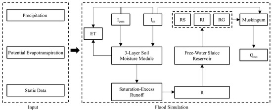
Figure 1.
The structure of the Grid-XAJ model.
We employed the trial-and-error method to optimize the model parameters. In detail, different parameter combinations were set in the Grid-XAJ model to simulate floods. The parameters are global optimal when evaluation metrics reach the global optimal values.
In this study, gauged rainfall was interpolated to each grid using the inverse distance weighting (IDW) method (Ir). The rainfall driving the Grid-XAJ model contains WRF-driven rainfall (Wr) and WRF-merged rainfall (Wm), which were obtained by merging Wr with gauged rainfall. PE for the Grid-XAJ model was calculated using the Penman–Monteith equation (PEPM). The input data for the Penman–Monteith equation, including radiation, temperature, pressure, humidity, and wind speed, were acquired from the WRF simulation.
2.3. Successive Correction Method
The successive correction method [45] is employed as a technique to refine forecast fields by incorporating gauged data. This approach can be traced back to the objective analysis method, initially proposed by Cressman in 1959. In this research, we utilized the successive correction method to merge the WRF-driven rainfall with gauged rainfall. The calculation steps are as follows.
The initial step of the successive correction method was to determine the initial field, for which we used the WRF-driven rainfall in our research. Subsequently, selecting an appropriate weight function becomes crucial. Notably, a variety of weight functions are offered to the successive correction method. We adopted Cressman’s circular scheme [45] as the weight function in this paper.
where Wij,k is the weight factor of grid (i, j) for rain station k; R is the influence radius, and is defined as the minimum value between the number of rows and columns within the WRF domain for each catchment; and dij,k is the distance from grid (i, j) to rainfall station k.
The subsequent step was acquiring the correction field, which was computed based on the gauged data and the forecasted data at the grid:
where C is the correction field, n is the total number of stations, Ek is the correction value of station k, Ok are the gauged data in station k, and Gk is the initial value in station k.
Finally, we obtained the analysis field based on the initial field and the correction field. Sometimes multiple iterations are necessary. In such instances, the current analysis field serves as the initial field for subsequent iteration. This study involved a total of five iterative corrections.
where A is the analysis field, and m is the number of iterative corrections, m = 5.
2.4. The Penman–Monteith Equation
Penman first established an evaporation model based on an energy balance equation [46]. Then, Monteith enhanced the model by using aero-dynamic conductance, which depends not only on wind speed, but also on surface ruggedness, atmospheric stability, and vegetation height [47]. This modified model is known as the Penman–Monteith model. In 1998, the experts and researchers of the Food and Agriculture Organization (FAO) updated and simplified the Penman–Monteith model by using some assumed constant parameters, such as a grass reference crop of height 0.12 m, a surface resistance of 70 s/m, and an albedo value of 0.23 [48].
The new equation for hourly potential evapotranspiration [49] is as follows:
where PEPM is the hourly potential evapotranspiration (mm/h); Rn is the net radiation at the crop surface (MJ/(m h)); G is the soil heat flux density (MJ/(m h)); Thr is the mean hourly air temperature at a 2 m height (°C); u2 is the wind speed at a 2 m height (m/s); is the saturation vapor pressure (kPa); ea is the actual vapor pressure (kPa); Δ is the slope of the vapor pressure curve (kPa/°C); and γ is the psychrometric constant, whose value is 0.066 kPa/°C. The parameters of the above equation are described below [49]:
where α is the surface albedo; ε is the surface emissivity; RS is the incoming short-wave radiation, W/m2; RL is the incoming long-wave radiation, W/m2; σ is the Stefan–Boltzmann constant, whose value is 5.67 × 10⁻⁸ W/(m2 K4); and Ts is the land surface temperature, K.
G is estimated as follows:
The WRF provides the wind speed (u10) at height h = 10 m, which can be converted to a 2 m wind speed:
is estimated as follows:
ea is estimated as follows [50]:
where q is the humidity, g/g, and p is the air pressure at 2 m, kPa.
Δ is estimated as follows:
2.5. Evaluation Methods and Metrics
The accuracy of rainfall, evapotranspiration, and streamflow is characterized using five assessment metrics: the correlation coefficient (RR) [51], the Nash–Sutcliffe efficiency coefficient (NSE) [52], the percent bias (PB) [53], Shannon entropy (SE) [54], and the time error of flow peak (TEP).
where Si are the simulated results for each time step i, Oi is the observed value, n is the total number of time series, x is a discrete random variable recording all different values in the grids, p(xk) is the frequency of the value of xk appearing in the grids, and N is the length of the x. The RR and NSE quantify the degree-of-fit between simulation and observation. PB measures the errors of the simulated results. In the case of single-value (such as rainfall peak) simulation output, PB represents the relative error between this value and the gauged value. The SE is regarded as a measure for spatial variability, and the higher its values are, the more complex the related spatial information is. The TEP is used to evaluate the time accuracy of the simulated flow peak.
The rainfall data were characterized in terms of three aspects: rainfall series, cumulative rainfall, and rainfall spatial distribution. Evaluation metrics including RR, NSE, and the PB of the rainfall peak (PBpr) were selected for analyzing the rainfall series [25]. For assessing the cumulative rainfall, the PB of the cumulative rainfall (PBcr) was selected as an evaluation metric. Due to the distinct spatial distributions of the three types of rainfall, SE was selected to evaluate their spatial characteristics [25]. For PEPM, we mainly focused on its spatial and temporal variations and possible influencing factors. The PB, NSE, PB of the flow peak (PBpf), and TEP were used to evaluate the flood simulations.
According to the Standard for Hydrological Information and Hydrological Forecasting (GB/T22482-2008) [55], if the PB ≤ 20%, the flood volume simulation is considered acceptable. Similarly, if the PBpf ≤ 20%, the flow peak simulation is considered acceptable. Additionally, the TEP within a three-hour window is deemed acceptable for peak occurrence time forecasting. The qualification rate (QR) of flood simulations can be determined as follows:
where n are the qualified events, and m are the total simulated events.
3. Study Area and Data
3.1. Study Catchments
The Tunxi catchment (29°27′ N~30°06′ N, 117°38′ E~118°30′ E) is located in the southeastern part of Anhui Province, with an area of 2670 km2. It has an elevation ranging from 92 m to 1622 m. The catchment is situated within a subtropical monsoon climate zone and experiences an average annual rainfall of approximately 1600 mm, making it a representative humid catchment. Rainfall is highly unevenly distributed throughout the year, with the months from April to June being rainy, which often leads to flood disasters, while the period from July to September experiences frequent drought. Farmland and woodland collectively occupy over 60% of the Tunxi catchment, with clay loam being the predominant soil type.
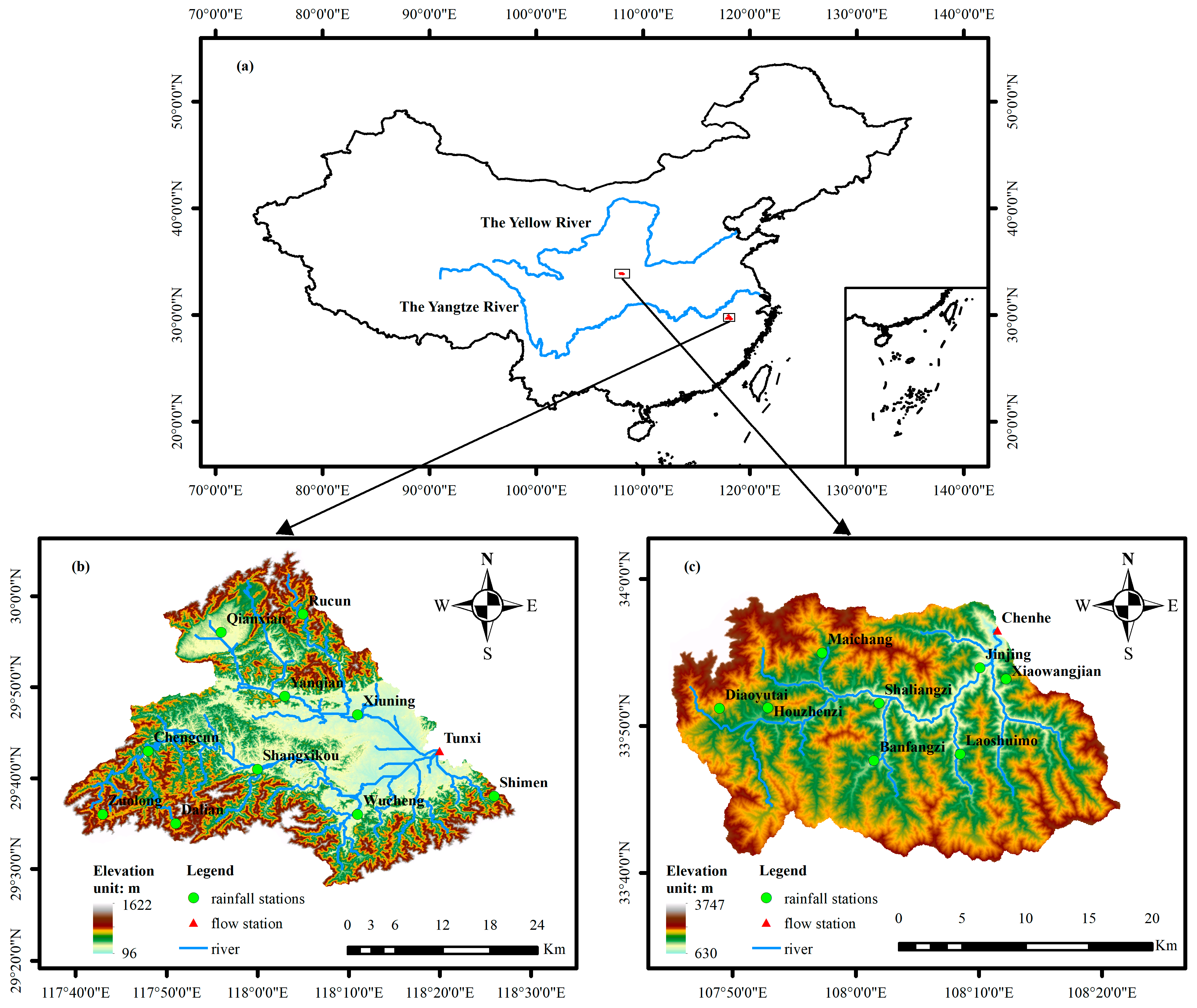
The Chenhe catchment (33°40′ N~34°01′ N, 107°42′ E~108°20′ E) is located in the central-southern part of Shaanxi Province, with an area of approximately 1380 km2 and elevations ranging from 600 m to 3800 m. This catchment represents a typical semi-humid catchment, with an annual runoff depth ranging from 100 to 500 mm and a multi-year average rainfall of 780 mm. The land use in the Chenhe catchment primarily consists of grassland, with a minor proportion of mixed forest and deciduous broadleaf forest. The predominant soil type is loam. The distribution of rivers and stations in the two catchments is shown in Figure 2.

Figure 2.
Study areas: (a) the location of the two catchments within China, (b) the channels and rainfall/discharge gauges of the Tunxi catchment, and (c) the channels and rainfall/discharge gauges of the Chenhe catchment.
3.2. Gauge Data
The hydrometeorological data for the Tunxi catchment, including daily evaporation, hourly discharge, and hourly precipitation, were provided by the Hydrology Bureau of Anhui Province. The catchment is equipped with eight rainfall stations and the Tunxi flow station. The Tunxi flow station, located at the catchment outlet, provided both rainfall and discharge data, while the rainfall stations only provided rainfall data. The evaporation data were obtained from the evaporation pan at the Tunxi flow station. We used twelve flood events for parameter calibration and six flood events for validation between 2012 and 2017. Then, four flood events were chosen to show the flood simulation performance of the WRF-driven Grid-XAJ model.
The Hydrology Bureau of Shaanxi Province provided the daily evaporation, hourly discharge, and 6 h precipitation data for the Chenhe catchment. Within this catchment, there are also eight rainfall stations and the Chenhe flow station. Some rainfall data and discharge data were sourced from the Tunxi flow station, and the rainfall stations only provided rainfall data. Evaporation was obtained via the evaporation pan at the Chenhe flow station. To determine the optimal model parameters in the Chenhe catchment, we utilized eight flood events for parameter calibration and four flood events for validation between 2003 and 2012. Similar to the Tunxi case study, we selected four flood events to show the flood simulation performance of the WRF-driven Grid-XAJ model. The initial state of the Grid-XAJ model was acquired after a warm-up period of a minimum of four months of daily flood simulation. Table 2 lists the selected events in the Tunxi and Chenhe catchments for driving the WRF-driven Grid-XAJ model.

Table 2.
The set of flood events.
3.3. FNL Data
The FNL(Final) Operational Global Analysis data provided by the National Centers for Environmental Prediction (NCEP) boast a high resolution and incorporate various observational and satellite-derived data. The FNL data are collected four times daily, the observations spanning the 6 h prior at least, and undergo global data analysis. They are widely utilized in numerical simulations and a range of weather analysis research [56,57]. For this study, FNL data from 2003 to 2017 were selected to provide the initial conditions for running the WRF model, with the FNL data being processed by the WPS.
4. Results and Discussion
4.1. Parameters Calibration
As explained before, a priori estimates of most model parameters were obtained from the underlying surface data. Then, the trial-and-error method was used to update the values of the parameters. The parameters that needed to be calibrated included K, C, Ci, Cg, Cs, and Lag, whose detailed description can be seen in reference [10]. For the Tunxi catchment, when all the flood evaluation metrics reached the global optimal values, the mean NSE for the eighteen flood events was 0.93 and the mean PB was 0.04. The QR of the flow peak was 94% and the QR of the peak occurrence time was 100%. For the Chenhe catchment, the mean NSE for the twelve flood events was 0.77 and the mean PB was 0.11. The QR of the flow peak was 94% and the QR of the peak occurrence time was 100%. The optimal values of K, C, Ci, Cg, Cs, and Lag are shown in Table 3. In addition, the simulation performance of the Grid-XAJ model in the Tunxi catchment was obviously better than that in the Chenhe catchment.

Table 3.
The optimal values of the parameters in two catchments.
4.2. Evaluation of Two Rainfall Products
Evaluating the Wr and Wm is crucial when analyzing the WRF-driven Grid-XAJ model. In this study, we regarded the Ir as the observed areal precipitation. The analysis focused on the rainfall series, cumulative rainfall, and rainfall spatial distribution.
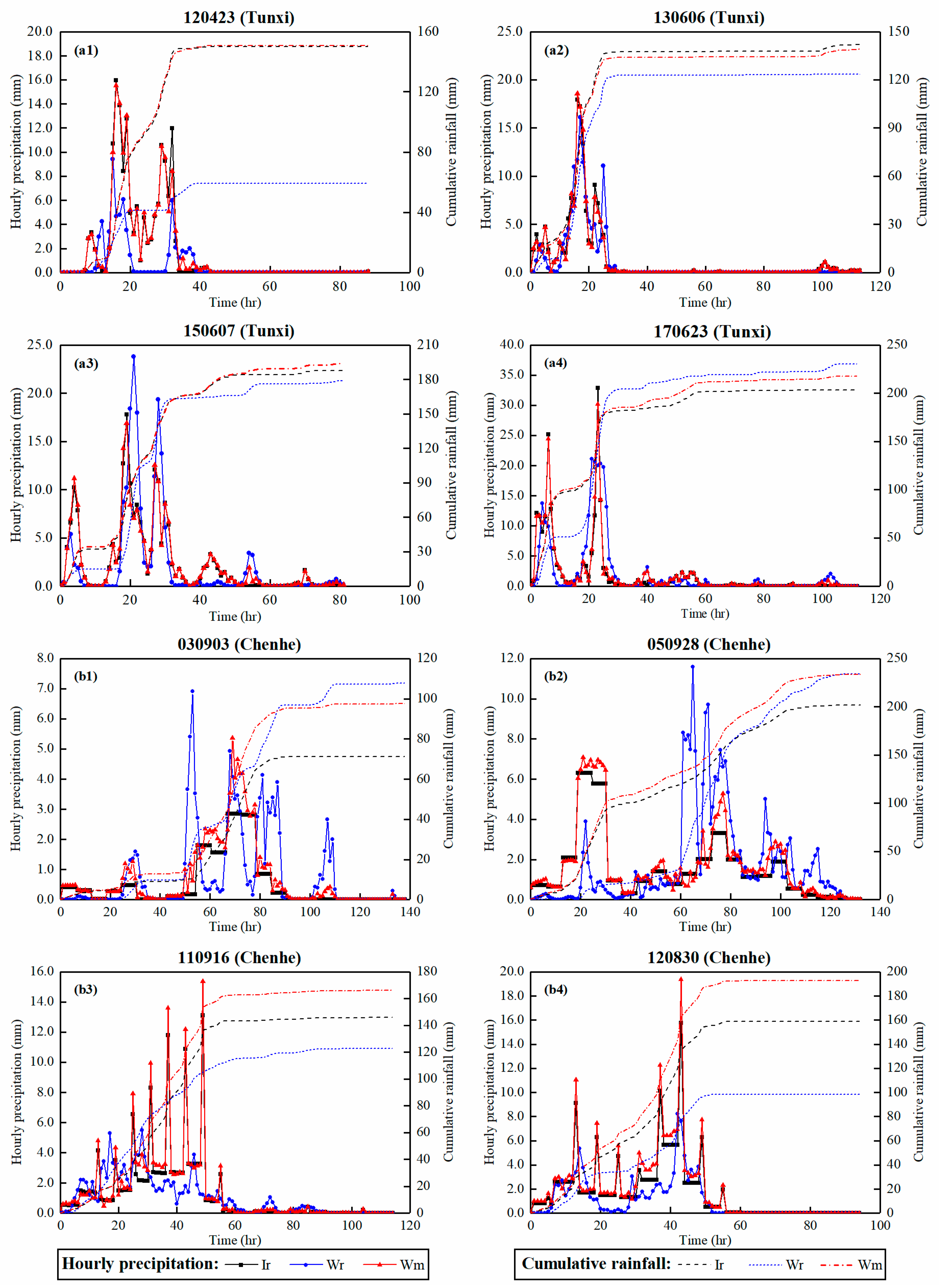
Table 4 displays the four evaluation metrics of the Wr and Wm. Figure 3 illustrates the hourly rainfall and cumulative rainfall. From Figure 3 and Table 4, Wr adequately simulates the real rainfall series but exhibits limitations in terms of the rainfall peak, cumulative rainfall, and degree-of-fit. Conversely, Wm significantly reduces the simulation errors, achieving a level of accuracy comparable to Ir.

Table 4.
The values of the four evaluation metrics of Wr and Wm.
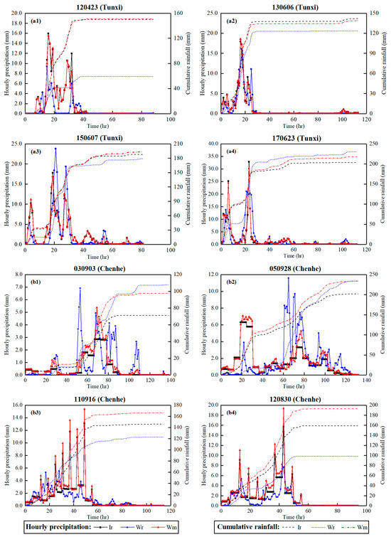
Figure 3.
Rainfall series: (a1–a4) show the hourly precipitation and cumulative rainfall for events 120423, 130606, 150607, and 170623 in the Tunxi catchment, and (b1–b4) show the hourly precipitation and cumulative rainfall for events 030903, 050928, 110916, and 120830 in the Chenhe catchment.
For the Tunxi catchment, the WRF model provided a reasonably accurate simulation of the rainfall series, with Wr showing a strong correlation with Ir (RR > 0.65). However, the degree-of-fit between Wr and Ir was unsatisfactory, as only event 130606 achieved a NSE value of 0.80, while the other three events achieved NSE values below 0.40. Notably, the WRF model successfully simulated all rainfall peaks, with all PBpr values being below 50%. Event 130606 exhibited a relatively large PBcr value of 60.1%, while the PBcr values for the other three events remained within 20%. Merging Wr with the gauged rainfall significantly improved rainfall accuracy, as indicated by Wm achieving higher RR values (>0.99). Furthermore, Wm demonstrated notable improvements in the degree-of-fit with Ir, exceeding all NSE values above 0.98. Additionally, the PBpr of Wm was substantially reduced to below 10%. In terms of cumulative rainfall analysis, there was a significant decrease in PBcr values across all four events, with values falling below 10%.
For the Chenhe catchment, the accuracy of Wr was relatively poor. Although Wr captures the rainfall series, its correlation with Ir was low, with only event 120830 achieving a RR value of 0.70. However, the RR values for the other three events were all below 0.50. Additionally, Wr exhibited a poor degree-of-fit with Ir, as indicated by NSE values below 0.50 for all four events. Moreover, the WRF model failed to accurately simulate rainfall peaks, for it generated non-existent peaks for events 030903 and 050928, and only partially simulated peaks for events 110916 and 120830. The PBpr of Wr for all four events exceeded 40%. Furthermore, the PBcr values were above 30% for events 030903 and 120830. After merging Wr and gauged rainfall, Wm achieved RR values of at least 0.95, with the NSE values all being above 0.75. The PBpr of Wm was noticeably reduced compared to that of Wr, and the PBcr values were also significantly decreased (<37%). In addition, the cumulative rainfall of Wm was consistently higher than that of Ir.
We further compared the rainfall of the Tunxi catchment and the Chenhe catchment. As shown in Table 4, the rainfall series, rainfall peaks, and cumulative rainfall in the Tunxi catchment outperformed the results in the Chenhe catchment. In the Tunxi catchment, the values of mean RR, mean NSE, mean PBpr, and mean PBcr were 0.75, 0.42, 30.0%, and 23.0% for Wr; and 0.99, 0.99, 4.8%, and 3.1% for Wm. In the Chenhe catchment, they were 0.43, −0.58, 83.0%, and 30.4% for Wr; and 0.98, 0.89, 34.7%, and 21.9% for Wm.
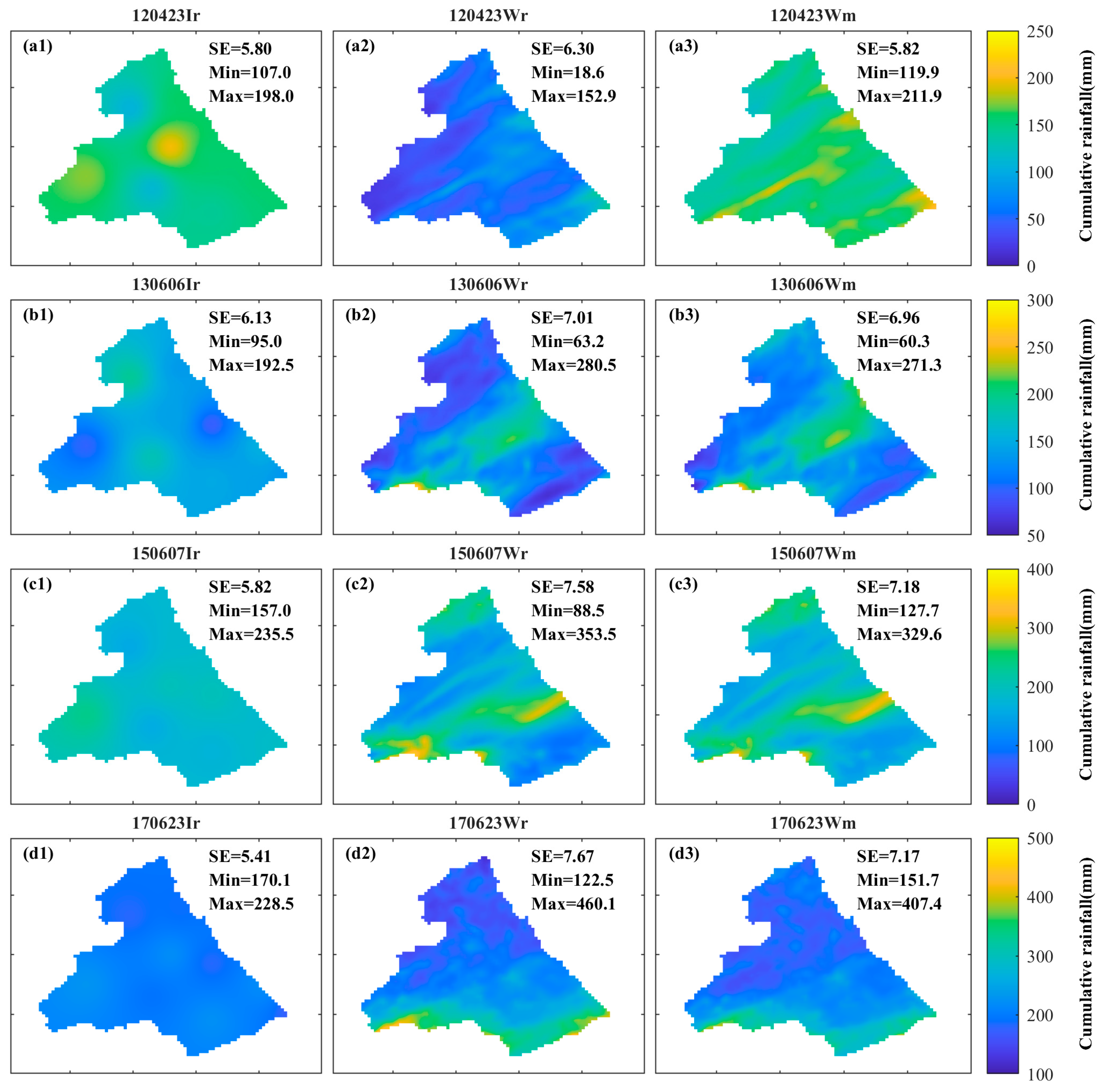
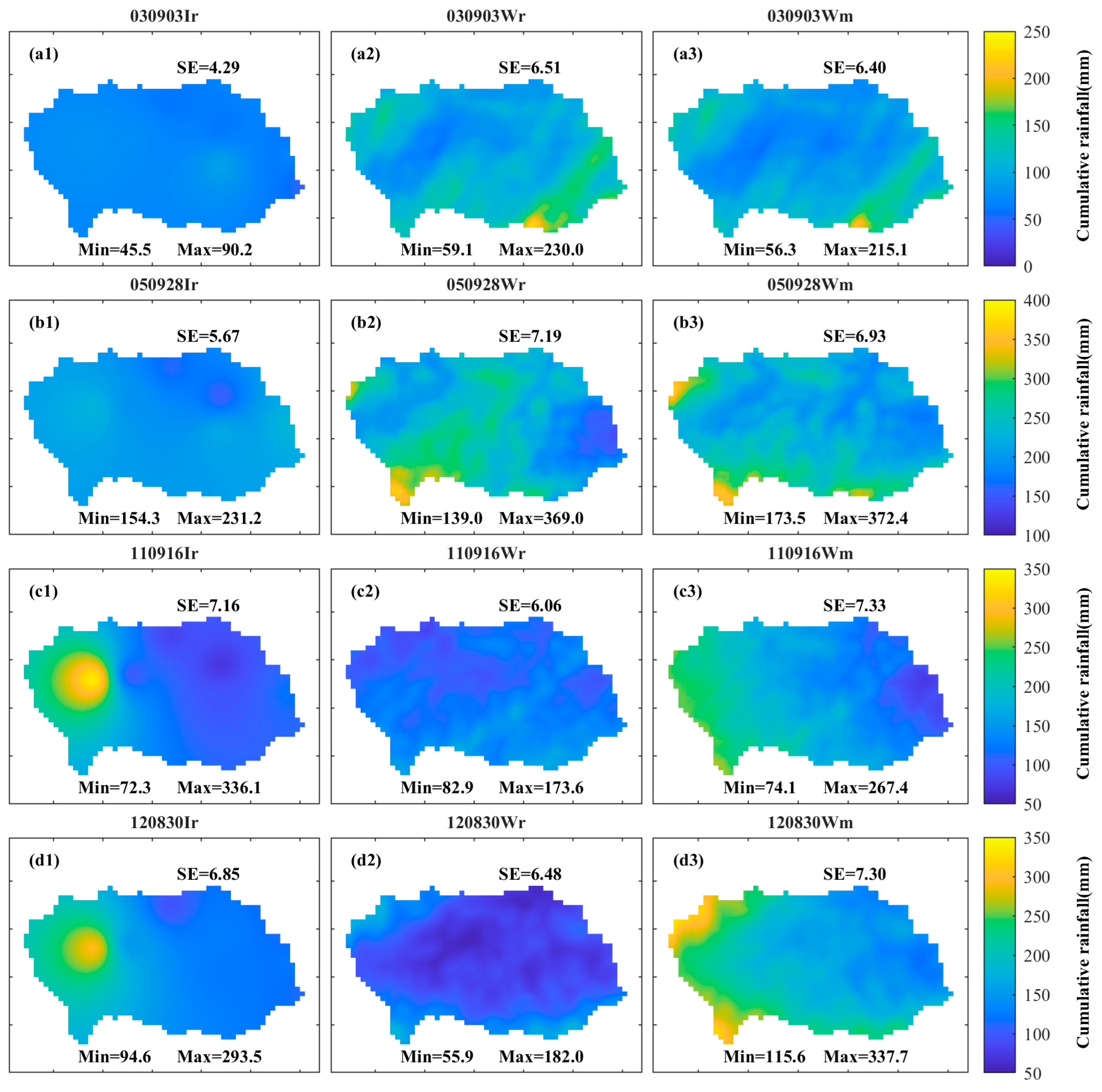
Figure 4 and Figure 5 present spatial distribution maps of the maximum cumulative rainfall in the two catchments. They demonstrate that Wm combines the advantages of both Ir and Wr. (1) The cumulative rainfall of Wm falls within most of the ranges of Ir and Wr. (2) The rainfall center of Ir is situated at the rain stations due to limitations imposed by the density and quality of gauged data. Wr can capture the rainfall center and spatial distribution details that rain stations fail to capture, but its spatial distribution and rainfall volume are not very accurate. Wm can incorporate rainfall centers from the other two rainfall products. (3) In both catchments, the spatial distribution of Ir is relatively smooth, and is closely related to the distribution of rainfall stations, resulting in simple spatial information. Wr exhibits a complex multi-banded spatial distribution. Wm also displays a multi-banded spatial distribution, but provides more detailed information compared to Ir, leading to a higher SE than that of Ir (0.3%~49.2%). When SE(Ir) < SE(Wr), merging Wr with Ir will simplify the spatial complexity of Wr. Conversely, when SE(Ir) > SE(Wr), merging Wr with Ir will enhance the spatial information.

Figure 4.
The spatial distribution of cumulative rainfall in the Tunxi catchment. The left panel (a1,b1,c1,d1) shows the spatial distribution of Ir, the middle panel (a2,b2,c2,d2) shows the spatial distribution of Wr, and the right panel (a3,b3,c3,d3) shows the spatial distribution of Wm.

Figure 5.
The spatial distribution of cumulative rainfall in the Chenhe catchment. The left panel (a1,b1,c1,d1) shows the spatial distribution of Ir, the middle panel (a2,b2,c2,d2) shows the spatial distribution of Wr, and the right panel (a3,b3,c3,d3) shows the spatial distribution of Wm.
4.3. Characteristics of PEPM
Due to the lack of observed areal PE, we made a concise analysis comparing PEPM and PEpan. Then, we mainly focused on some influence factors for PEPM and its spatiotemporal distribution characteristics.
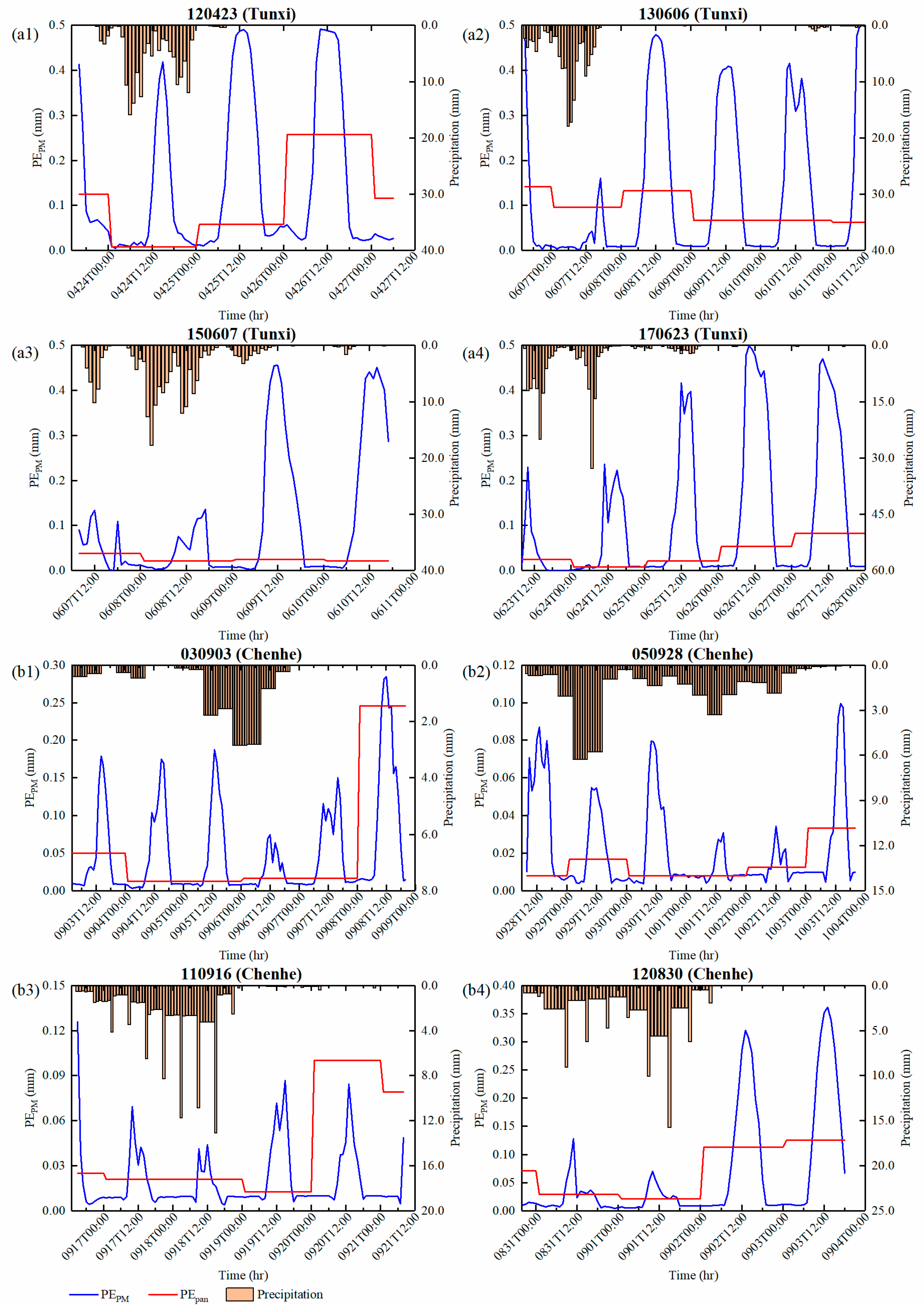
Figure 6 presents a comparison between the PEPM and PEpan series. As shown in the figure, PEpan remains stable throughout the day, with sudden changes occurring only at the transition to the next day. Contrarily, PEPM exhibits hourly variations and changes gradually over time. In addition, the range of PEPM (0.0 mm~0.5 mm for the Tunxi catchment, 0.0 mm~0.4 mm for the Chenhe catchment) is greater than that of PEpan (0.0 mm~0.3 mm for the Tunxi catchment, 0.0 mm~0.25 mm for the Chenhe catchment).
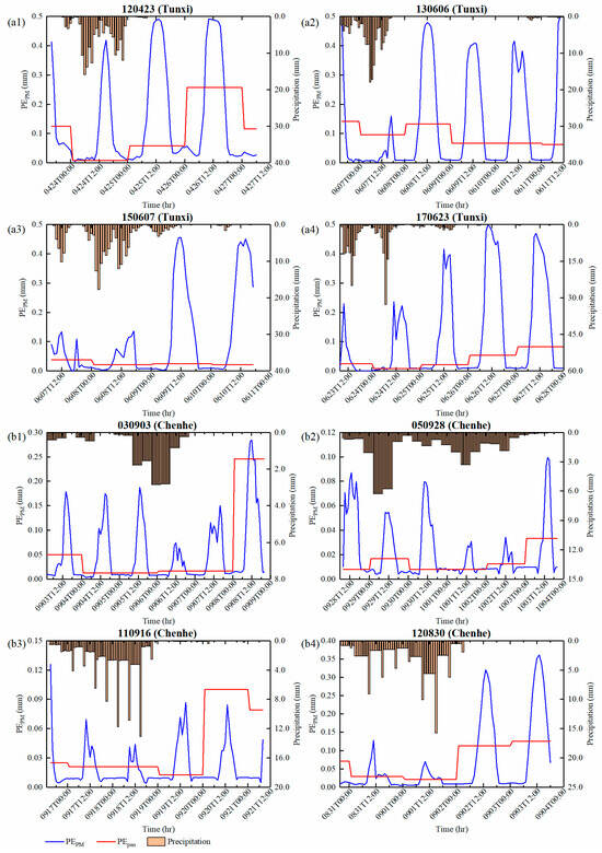
Figure 6.
The PEPM series: (a1–a4) show the hourly PEPM of events 120423, 130606, 150607, and 170623 in the Tunxi catchment, and (b1–b4) show the hourly PEPM of events 030903, 050928, 110916, and 120830 in the Chenhe catchment.
As shown in Figure 6, rainfall significantly influences PEPM. PEPM notably decreases during rainy periods in both catchments. Moreover, the influence of different climatic zones is evident in the PEPM values. The PEPM values in the Tunxi catchment are considerably higher compared to those in the Chenhe catchment. Specifically, in the Tunxi catchment, the PEPM values range from 0.0 to 0.5 mm. In the Chenhe catchment, the PEPM values range from 0.0 to 0.2 mm for events 050928 and 110916, and from 0.0 to 0.4 mm for the other two events.
PEPM exhibits distinct temporal distribution characteristics. As illustrated in Figure 6, evapotranspiration mainly occurs between 6:00 a.m. and 6:00 p.m., with the peak PEPM occurring around noon at 12:00 p.m. During the nighttime, the PEPM values approach zero.
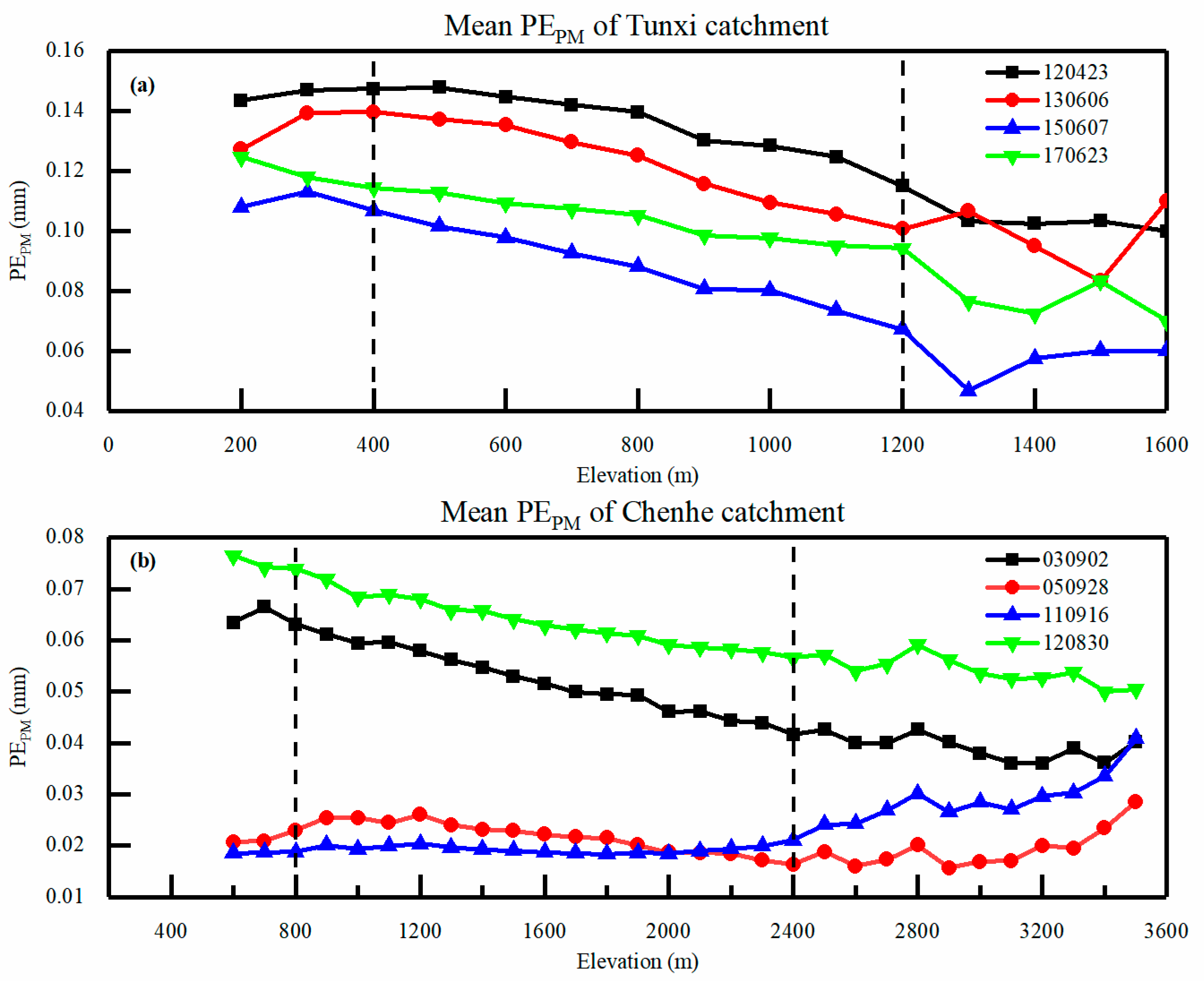
PEPM exhibits distinct spatial distribution characteristics. Figure 7 depicts the spatial distribution of the mean PEPM, where the mean PEPM refers to the average spatial distribution of PEPM over all time periods. The SE values exceed 2.0 for the Tunxi catchment and surpass 3.0 for the Chenhe catchment. Figure 8 illustrates the relationship between the mean PEPM and elevation. As shown in Figure 8, there is a relationship between PEPM and elevation: regions with higher elevations display relatively lower mean PEPM values, while areas with moderate elevations exhibit the highest mean PEPM values, and slightly lower values are observed in lower elevation areas. Here are the specifics: (1) In the lower elevation areas of the catchment, the mean PEPM is moderately high. Within the 0~400 m elevation range in the Tunxi catchment, except for event 170623, there is a slight increase in the mean PEPM with higher elevations. Similarly, within the 600~800 m elevation range in the Chenhe catchment, except for event 120830, there is also a slight increase in the mean PEPM with higher elevations. Although the mean PEPM values of event 170623 in the Tunxi catchment and event 120830 in the Chenhe catchment decreased with increasing elevation, it is worth noting that some lower elevation areas, such as rivers near the catchment outlets, exhibit a relatively low mean PEPM. (2) In the middle elevation areas of the catchment, the mean PEPM is the highest. Within the 400~1200 m elevation range of the Tunxi catchment, there is a gradual decrease in the mean PEPM as the elevation increases. Similarly, within the 800~2400 m elevation range of the Chenhe catchment, although there is a fluctuating trend in the mean PEPM with increasing elevation for event 110916, for the other three events, there is a gradual decrease in the mean PEPM with higher elevations. (3) In the high elevation areas of the catchment, the mean PEPM is the lowest. In the regions with an elevation above 2400 m in the Chenhe catchment and above 1200 m elevation in the Tunxi catchment, the mean PEPM exhibits a fluctuating pattern. For all events, as the mean PEPM decreases to a certain extent with increasing elevation, it then shows an upward trend. The possible reason for this phenomenon is that PE is mainly affected by wind speed in the middle and low elevations of the catchment, while PE is mainly affected by temperature in the high elevations of the catchment.
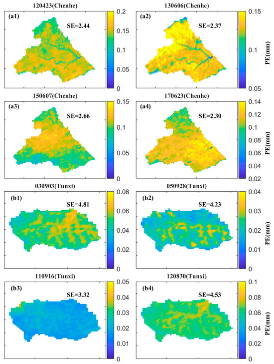
Figure 7.
The spatial distribution of PEPM: (a1–a4) show the spatial distribution of the mean PEPM for events 120423, 130606, 150607, and 170623 in the Tunxi catchment, and (b1–b4) show the spatial distribution of the mean PEPM for events 030903, 050928, 110916, and 120830 in the Chenhe catchment.
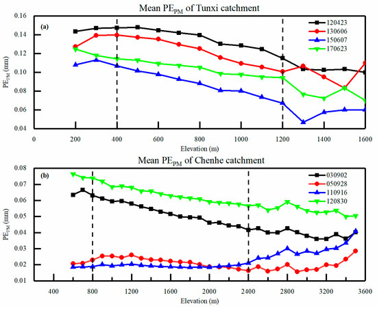
Figure 8.
The relationship between the mean PEPM and DEM in the Tunxi catchment (a) and in the Chenhe catchment (b).
4.4. Evaluation of Discharge
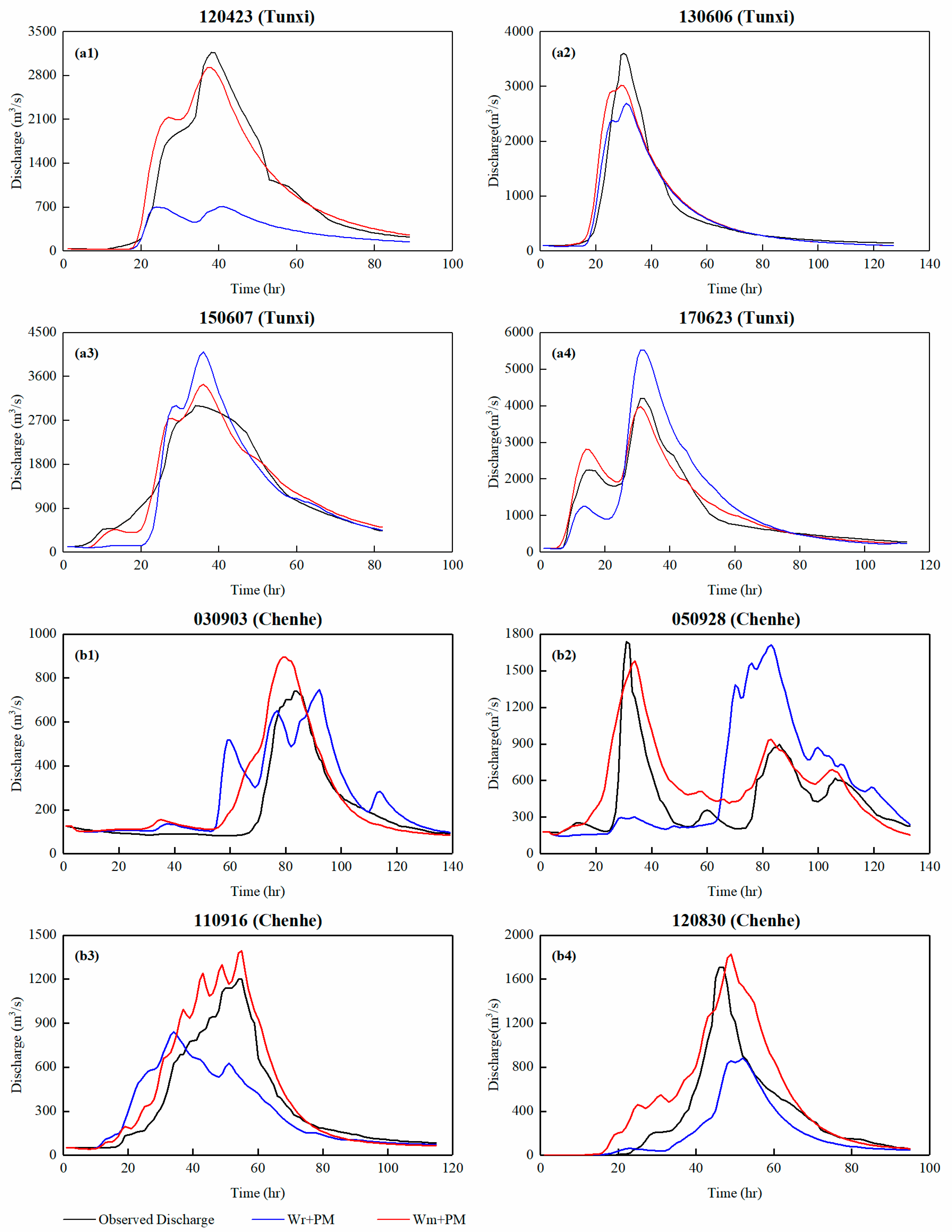
Different from the traditional Grid-AXJ model, Wr and Wm were used as input rainfall to drive the Grid-XAJ model for flood forecasting in this paper. Furthermore, we considered substituting PEpan with PEPM in the model. The results are presented in Figure 9. Table 5 shows the values of the metrics used for the simulated floods. It is evident from Figure 9 and Table 5 that directly using Wr and PEPM to simulate floods yields unsatisfactory results. However, incorporating Wm as input rainfall significantly enhances the forecasting performance.
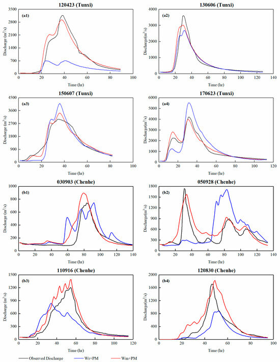
Figure 9.
The hydrograph of flood events: (a1–a4) show the flood hydrograph of events 120423, 130606, 150607, and 170623 in the Tunxi catchment, and (b1–b4) show the flood hydrograph of events 030903, 050928, 110916, and 120830 in the Chenhe catchment.

Table 5.
The evaluation metrics of the simulated floods.
To evaluate the flood forecasting capability of the WRF-driven Grid-XAJ model, Wr + PEPM and Wm + PEPM forcing scenarios were designed for the Grid-XAJ model. In the Tunxi catchment, for scenario Wr + PEPM, only one flood event exhibits an NSE value exceeding 0.90. The PB values are relatively small for events 130606 and 150607. However, for the other two events, particularly event 120423, the PB values are significantly larger. All simulated flow peaks fail to meet the qualification criteria, with all PBpf values exceeding 20%, despite having a small TEP. For scenario Wm + PEPM, all NSE values surpass 0.90. The flood volume simulation is robust, with all PB values below 5%. For flow peaks, the PBpf values for all four events are below 20%, with events 130606 and 170623 achieving PBpf values below 10%. The TEP for the four floods remain within a 3 h margin, demonstrating significant reductions compared to scenario Wr + PEPM.
In the Chenhe catchment, for scenario Wr + PEPM, the NSE values for all events remain below 0.55, indicating a suboptimal degree-of-fit between the simulation and observation. Except for event 110916, all PB values exceed 20%. Additionally, notable deficiencies are observed in peak flows. Although the PBpf values of events 030903 and 050928 meet the criteria, significant temporal discrepancies exist for the TEP (−9 h, −42 h). For events 110916 and 120830, neither the flow peaks nor the peak occurrence times align with the gauged discharges. For scenario Wr + PEPM, all four events achieve NSE values surpassing 0.5. Although event 030903 does not meet the criteria for PBpf and TEP, these deviations are relatively small. The other three events yield satisfactory results in terms of PBpf and TEP.
To further illustrate the impact of merging the method of rainfall on flood forecasting, we compared the streamflow simulations of the Grid-XAJ model under two forcing scenarios. It is clear that scenario Wm + PEPM significantly improves the degree-of-fit, flood volume, and flow peaks over scenario Wr + PEPM. In the Tunxi catchment, compared to scenario Wr + PEPM, the mean NSE value of scenario Wm + PEPM increased by 0.3, the mean PB value decreased from 21.5% to 3.5%, the QR of PBpf increased from 0 to 100%, and the TEP decreased one hour. In the Chenhe catchment, compared to scenario Wr + PEPM, the NSE value of scenario Wm + PEPM increased from −1.65~0.54 to 0.54~0.87. The PB values exhibit minor fluctuations, with reductions of 8.26% and 0.89% for events 030903 and 120830, and a slight increase of 1.6% and 2.77% for events 050928 and 110916. The QR of PBpf increased from 50% to 100% and the TEP decreased by seventeen hours.
We further compared the flood simulations of the WRF-driven Grid-XAJ model in different climatic catchments. For scenario Wr + PEPM, the mean NSE value in the Tunxi catchment is 66.4% higher than that in the Chenhe catchment, and the mean PB is 7.3% lower than that in the Chenhe catchment. Additionally, the QR of the TEP is 100% in the Tunxi catchment but 0% in the Chenhe catchment. For scenario Wr + PEPM, all NSE values exceed 0.90 in the Tunxi catchment, whereas in the Chenhe catchment, all NSE values fall below 0.90. In the Tunxi catchment, the QRs for PB, PBpf, and TEP are all 100%, while in the Chenhe catchment, the QRs for the PB, PBpf, and TEP are 50%, 75%, and 75%, respectively. These outcomes indicate that the results of the model in the semi-humid catchment can only serve as a reference.
4.5. Discussion
We built a WRF-driven Grid-XAJ model, fully considering the influence of meteorology to enhance the accuracy of flood simulations. The traditional forcing scenario of spatial interpolation rainfall and pan evaporation renders the Grid-XAJ model inapplicable in regions with limited rainfall data and neglects other meteorological variables. Additionally, their spatiotemporal accuracy may be affected by many factors. In this study, we fully considered the influence of meteorology on the Grid-XAJ model compared with Yao [24] and Meng [38], though the forcing scenarios in their studies do improve the accuracy of flood forecasting. Using the successive correction method actually enhanced the spatiotemporal accuracy of Wr distribution (Table 4), which was consistent with other studies that used this method to improve rainfall accuracy [58]. PEPM, which exhibited a reasonable spatiotemporal distribution (Figure 7 and Figure 8), was also consistent with other research that used it with NWM output for PE calculation [59].
Table 4 shows that Wr and Wm performed better in the Tunxi catchment than in the Chenhe catchment. This can be attributed to the fact that the humid catchment typically experiences more intense rainfall with shorter durations, and the WRF model performs better in short-term heavy rainfall forecasting rather than long-term light rainfall. Additionally, errors in the WRF-driven rainfall can partly reflect the performance of the WRF-driven Grid-XAJ model (Figure 3 and Figure 9). The NSE values of Wm are higher than those of Wr, suggesting that Wm may exhibit better performance in degree-of-fit for simulated floods. Errors in the peak rainfall can lead to inaccurate predictions of the peak flood. The application of Wm enhances the PBpr of Wr, which positively influences the simulation of flow peaks. An accurate estimate for the cumulative rainfall will improve the precision of simulated flood volume. The error in the cumulative rainfall of Wm is smaller than that of Wr, which indicates that Wm is more suitable to simulate flood volume than Wr. In addition, the error of each metric for Wr and Wm in the Tunxi catchment is lower than that in the Chenhe catchment, suggesting that the Grid-XAJ model may yield more accurate flood simulations in the Tunxi catchment. Figure 6 shows that PEPM exhibits a correlation with rainfall. This association can be attributed to the concurrent decrease in air temperature and increase in moisture content during rainy periods. Furthermore, PEPM in the Tunxi catchment was higher compared to that in the Chenhe catchment (Figure 6). This may be attributed to the elevated soil moisture content and a greater availability of water vapor within the humid catchment. Research has shown a strong correlation between PEPM and elevation [60], and that was proved in our study (Figure 7).
As mentioned in Section 2.2, the Grid-XAJ model adopts the saturation-excess runoff module to calculate runoff generation, which represents the main runoff generation mode in humid catchments [61]. The runoff generation mode of a semi-humid catchment is intricate and potentially encompasses various other modes of runoff generation. Thus, the Grid-XAJ model appears to be better suited for a humid watershed.
5. Conclusions
Based on gauged rainfall, WRF-driven rainfall (Wr), and meteorological data output by WRF, WRF-merged rainfall (Wm) and potential evapotranspiration calculated using the Penman–Monteith equation (PEPM) were utilized in this paper. Then, two forcing scenarios (Wr + PEPM and Wm + PEPM) were designed to drive the Grid-XAJ model in both the Tunxi and the Chenhe catchments, aiming to enhance the accuracy of flood simulations. The main conclusions are as follows.
The accuracy of Wm surpasses that of Wr in both humid and semi-humid catchments, indicating a more rational spatial distribution than Ir. Wm also incorporates rainfall centers from both Wr and Ir. PEPM demonstrates significant spatiotemporal heterogeneity, exhibiting hourly variations compared to PEpan. Additionally, PEPM can be influenced by rainfall, and its values are higher in the humid catchment than in the semi-humid catchment. The spatial distribution of PEPM exhibits a gradual decrease from moderately elevated regions towards areas characterized by both higher and lower elevations.
The WRF-driven Grid-XAJ model holds significant potential in flood forecasting. The Grid-XAJ model, when driven by scenario Wr + PEPM, shows a broad capacity to simulate floods. In contrast, under scenario Wm + PEPM, the model demonstrates a superior flood forecasting performance. Additionally, the WRF-driven Grid-XAJ model demonstrates superior flood forecasting performance in the humid catchment compared to the semi-humid catchment.
6. Study Limitations and Prospects
In this study, the rainfall inputs into the Grid-XAJ model included WRF-driven rainfall and WRF-merged rainfall, which are based on FNL data and gauged data, thereby not extending the lead time of flood forecasting. In addition, we examined the influence of meteorological factors on hydrological processes, but the feedback of hydrological factors on meteorological processes was not considered. In future studies, we will try to extend the lead time by using forecasted data (i.e., GFS data) to drive the WRF model and improve the accuracy of the WRF-forecast rainfall before it is used to drive the Grid-XAJ model. Furthermore, we will explore methods to realize the two-way coupling between the WRF model and the Grid-XAJ model.
Author Contributions
Conceptualization, J.G. (Junchao Gong), Y.H. and C.Y.; methodology, J.G. (Junchao Gong); validation, J.G. (Junchao Gong), Y.H. and C.Y.; software, J.G. (Junchao Gong), Y.H., M.S. and J.G. (Junfu Gong); formal analysis, Y.H., Y.M. and Z.S.; investigation, J.G. (Junchao Gong), Y.H. and C.Y.; resources, Y.M., M.S. and J.G. (Junfu Gong); data curation, J.G. (Junchao Gong), Y.M., M.S. and J.L.; writing—original draft preparation, J.G. (Junchao Gong); writing—review and editing, J.G. (Junchao Gong), Y.H., C.Y., Y.M., M.S. and J.G. (Junfu Gong); visualization, Y.M., M.S. and Z.S.; supervision, Y.H., C.Y. and J.L.; project administration, Y.M., J.G. (Junfu Gong) and Z.S.; funding acquisition, Y.H. and C.Y. All authors have read and agreed to the published version of the manuscript.
Funding
This work was funded by the National Key R&D Program of China (Grant No. 2021YFB3900601), the National Natural Science Foundation of China (Grant Nos. 51979070 and 52079035), the Key Science and Technology Program of Ministry of Water Resources of China (SKR-2022032), and the Natural Science Foundation of Anhui Province of China (Grant No. 2208085US06).
Data Availability Statement
Data will be made available upon request.
Acknowledgments
The authors thank Li Anqi for his guidance on the calibration of the Grid-XAJ model.
Conflicts of Interest
Author Mingkun Sun was employed by the company Yellow River Engineering Consulting Co., Ltd. The remaining authors declare that the research was conducted in the absence of any commercial or financial relationships that could be construed as a potential conflict of interest.
References
- Lei, T.J.; Wang, J.B.; Li, X.Y.; Wang, W.W.; Shao, C.L.; Liu, B.Y. Flood Disaster Monitoring and Emergency Assessment Based on Multi-Source Remote Sensing Observations. Water 2022, 14, 2207. [Google Scholar] [CrossRef]
- Bu Daher, J.; Huygue, T.; Stolf, P.; Hernandez, N. An Ontology and a reasoning approach for Evacuation in Flood Disaster Response. J. Inf. Knowl. Manag. 2023, 22, 2350042. [Google Scholar] [CrossRef]
- Cao, Y.T.; Sun, X.H. Application of Shuangchao hydrological model in Shanxi semiarid and semi-humid area. In Proceedings of the 2011 International Conference on Artificial Intelligence and Computational Intelligence (AICI 2011), Taiyuan, China, 23–25 September 2011; pp. 84–91. [Google Scholar]
- Gong, J.F.; Yao, C.; Li, Z.J.; Chen, Y.; Huang, Y.C.; Tong, B.X. Improving the flood forecasting capability of the Xinanjiang model for small-and medium-sized ungauged catchments in South China. Nat. Hazards 2021, 106, 2077–2109. [Google Scholar] [CrossRef]
- Gong, J.F.; Weerts, A.H.; Yao, C.; Li, Z.J.; Huang, Y.C.; Chen, Y.F.; Chang, Y.F.; Huang, P.N. State updating in a distributed hydrological model by ensemble Kalman filtering with error estimation. J. Hydrol. 2023, 620, 129450. [Google Scholar] [CrossRef]
- Jeziorska, J.; Niedzielski, T. Applicability of TOPMODEL in the mountainous catchments in the upper Nysa Kłodzka river basin (SW Poland). Acta Geophys. 2018, 66, 203–222. [Google Scholar] [CrossRef]
- Breinl, K. Driving a lumped hydrological model with precipitation output from weather generators of different complexity. Hydrol. Sci. J. 2016, 61, 1395–1414. [Google Scholar] [CrossRef]
- Taheri, M.; Shamsi Anboohi, M.; Nasseri, M.; Mbdolmajid, A. Developing a dynamic semi-distributed hydrological model considering interactions between soil moisture and evapotranspiration: Application of bulk transfer method. Hydrol. Sci. J. 2023, 68, 228–245. [Google Scholar] [CrossRef]
- Beven, K.; Binley, A. The future of distributed models: Model calibration and uncertainty prediction. Hydrol. Process. 1992, 6, 279–298. [Google Scholar] [CrossRef]
- Yao, C.; Li, Z.J.; Yu, Z.B.; Zhang, K. A priori parameter estimates for a distributed, grid-based Xinanjiang model using geographically based information. J. Hydrol. 2012, 468–469, 47–62. [Google Scholar] [CrossRef]
- Yao, C.; Li, Z.J.; Bao, H.J.; Yu, Z.B. Application of a developed Grid-Xinanjiang model to Chinese watersheds for flood forecasting purpose. J. Hydrol. Eng. 2009, 14, 923–934. [Google Scholar] [CrossRef]
- Liu, Q.; Wan, D.S.; Yu, Y.F.; Zhang, Y.M. Research and application of the parallel computing method for the grid-based Xin’anjiang model. Hydrol. Res. 2023, 54, 591–605. [Google Scholar] [CrossRef]
- Dembélé, M.; Hrachowitz, M.; Savenije, H.H.; Mariéthoz, G.; Schaefli, B. Improving the predictive skill of a distributed hydrological model by calibration on spatial patterns with multiple satellite data sets. Water Resour. Res. 2020, 56, e2019WR026085. [Google Scholar] [CrossRef]
- Wu, L.; Liu, X.; Yang, Z.; Yu, Y.; Ma, X.Y. Effects of single- and multi-site calibration strategies on hydrological model performance and parameter sensitivity of large-scale semi-arid and semi-humid watersheds. Hydrol. Process. 2022, 36, e14616. [Google Scholar] [CrossRef]
- Shin, M.J.; Jung, Y. Using a global sensitivity analysis to estimate the appropriate length of calibration period in the presence of high hydrological model uncertainty. J. Hydrol. 2022, 607, 127546. [Google Scholar] [CrossRef]
- Guo, W.J.; Wang, C.H.; Ma, T.F.; Zeng, X.M.; Yang, H. A distributed Grid-Xinanjiang model with integration of subgrid variability of soil storage capacity. Water Sci. Eng. 2016, 9, 97–105. [Google Scholar] [CrossRef]
- Zhang, S.T.; Zhang, J.Z.; Liu, Y.; Liu, Y.C. A mathematical spatial interpolation method for the estimation of convective rainfall distribution over small watersheds. Environ. Eng. Res. 2016, 21, 226–232. [Google Scholar] [CrossRef]
- Hu, Q.F.; Li, Z.; Wang, L.Z.; Huang, Y.; Wang, Y.T.; Li, L.J. Rainfall spatial estimations: A review from spatial interpolation to multi-source data merging. Water 2019, 11, 579. [Google Scholar] [CrossRef]
- Zhang, M.; Chen, Y. Link prediction based on graph neural networks. In Proceedings of the International Conference on Neural Information Processing, Siem Reap, Cambodia, 13–16 December 2018; pp. 5171–5181. [Google Scholar]
- Wu, Y.; Zhuang, D.; Labbe, A.; Sun, L. Inductive Graph Neural Networks for Spatiotemporal Kriging. In Proceedings of the AAAI Conference on Artificial Intelligence, Vancouver, BC, Canada, 2–9 February 2021; 35, pp. 4478–4485. [Google Scholar] [CrossRef]
- Li, J.; Shen, Y.; Chen, L.; Ng, C.W.W. Rainfall Spatial Interpolation with Graph Neural Networks. In Proceedings of the International Conference on Database Systems for Advanced Applications, Tianjin, China, 17–20 April 2023; Springer: Cham, Switzerland, 2023; pp. 175–191. [Google Scholar] [CrossRef]
- Wang, Y.; Gueye, M.; Greybush, S.J.; Greatrex, H.; Whalen, A.J.; Ssentongo, P.; Zhang, F.Q.; Jenkins, G.S.; Schiff, S.J. Verification of operational numerical weather prediction model forecasts of precipitation using satellite rainfall estimates over Africa. Meteorol. Appl. 2023, 30, e2112. [Google Scholar] [CrossRef]
- Caldwell, P.; Chin, H.N.S.; Bader, D.C.; Bala, G. Evaluation of a WRF dynamical downscaling simulation over California. Climatic Chang. 2009, 95, 499–521. [Google Scholar] [CrossRef]
- Yao, C.; Ye, J.Y.; He, Z.X.; Bastola, S.; Zhang, K.; Li, Z.J. Evaluation of flood prediction capability of the distributed Grid-Xinanjiang model driven by weather research and forecasting precipitation. J. Flood Risk Manag. 2019, 12, e12544. [Google Scholar] [CrossRef]
- Sun, M.K.; Li, Z.J.; Yao, C.; Liu, Z.Y.; Wang, J.F.; Hou, A.Z.; Zhang, K.; Huo, W.B.; Liu, M.Y. Evaluation of Flood Prediction Capability of the WRF-Hydro Model Based on Multiple Forcing Scenarios. Water 2020, 12, 874. [Google Scholar] [CrossRef]
- Tewari, M.; Chen, F.; Dudhia, J.; Ray, P.; Miao, S.G.; Nikolopoulos, E.; Treinish, L. Understanding the sensitivity of WRF hindcast of Beijing extreme rainfall of 21 July 2012 to microphysics and model initial time. Atmos. Res. 2022, 271, 106085. [Google Scholar] [CrossRef]
- Li, J.; Yuan, D.; Sun, Y.; Li, J. Comparing the performances of WRF QPF and PERSIANN-CCS QPEs in karst flood simulations and forecasting by coupling the Karst-Liuxihe model. Front. Earth Sci. 2022, 16, 381–400. [Google Scholar] [CrossRef]
- Yaremchuk, M.; Nechaev, D.; Panteleev, G. A Method of Successive Corrections of the Control Subspace in the Reduced-Order Variational Data Assimilation. Mon. Weather Rev. 2009, 137, 2966–2978. [Google Scholar] [CrossRef]
- Cui, Y.K.; Song, L.S.; Fan, W.J. Generation of spatio-temporally continuous evapotranspiration and its components by coupling a two-source energy balance model and a deep neural network over the Heihe River Basin. J. Hydrol. 2021, 597, 126176. [Google Scholar] [CrossRef]
- Jaafar, H.H.; Mourad, R.M.; Kustas, W.P.; Anderson, M.C. A Global Implementation of Single- and Dual-Source Surface Energy Balance Models for Estimating Actual Evapotranspiration at 30-m Resolution Using Google Earth Engine. Water Resour. Res. 2022, 58, e2022WR032800. [Google Scholar] [CrossRef]
- Jiang, Y.Z.; Tang, R.L.; Li, Z.L. A framework of correcting the angular effect of land surface temperature on evapotranspiration estimation in single-source energy balance models. Remote Sens. Environ. 2022, 283, 113306. [Google Scholar] [CrossRef]
- Du, J.Z.; Xu, X.L.; Liu, H.X.; Wang, L.Y.; Cui, B.S. Deriving a high-quality daily dataset of large-pan evaporation over China using a hybrid model. Water Res. 2023, 238, 120005. [Google Scholar] [CrossRef]
- Basu Roy, T.; Dutta, D.; Chakrabarty, A. Spatio-temporal variation of evapotranspiration derived from multi-temporal landsat datasets using fao-56 penman-monteith method. In Spatial Modeling in Forest Resources Management: Rural Livelihood and Sustainable Development; Shit, P.K., Pourghasemi, H.R., Eds.; Springer: Cham, Switzerland, 2021; pp. 405–423. [Google Scholar] [CrossRef]
- Ghafourian, S.; Aminnejad, B.; Ebrahimi, H. Evaluating Direct Assimilation of Satellite-Based Potential Evapotranspiration into SWAT for Improving Hydrological Modeling. J. Hydrol. Eng. 2023, 28, 05023019. [Google Scholar] [CrossRef]
- Jiang, S.; Wei, L.; Ren, L.; Xu, C.Y.; Zhong, F.; Wang, M.; Zhang, L.Q.; Yuan, F.; Liu, Y. Utility of integrated IMERG precipitation and GLEAM potential evapotranspiration products for drought monitoring over mainland China. Atmos. Res. 2021, 247, 105141. [Google Scholar] [CrossRef]
- Akar, F.; Katipoğlu, O.M.; Yeşilyurt, S.N.; Taş, M.B.H. Evaluation of tree-based machine learning and deep learning techniques in temperature-based potential evapotranspiration prediction. Polish. J. Environ. Stud. 2023, 32, 1009–1023. [Google Scholar] [CrossRef] [PubMed]
- Mostafa, R.R.; Kisi, O.; Adnan, R.M.; Sadeghifar, T.; Kuriqi, A. Modeling potential evapotranspiration by improved machine learning methods using limited climatic data. Water 2023, 15, 486. [Google Scholar] [CrossRef]
- Meng, C.; Zhou, J.; Zhong, D.; Wang, C.; Guo, J. An Improved Grid-Xinanjiang Model and Its Application in the Jinshajiang Basin, China. Water 2018, 10, 1265. [Google Scholar] [CrossRef]
- Ai, G.; Wang, S.; Zhi, H. Simulations of a Heavy Snowfall Event in Xinjiang via the WRF Model Coupled with Different Land Surface Parameterization Schemes. Atmosphere 2023, 14, 1376. [Google Scholar] [CrossRef]
- Tiwari, G.; Kumar, P. Predictive skill comparative assessment of WRF 4DVar and 3DVar data assimilation: An Indian Ocean tropical cyclone case study. Atmos. Res. 2022, 277, 106288. [Google Scholar] [CrossRef]
- Thompson, G.; Field, P.R.; Rasmussen, R.M.; Hall, W.D. Explicit forecasts of winter precipitation using an improved bulk microphysics scheme. Part II: Implementation of a new snow parameterization. Mon. Weather Rev. 2008, 136, 5095–5115. [Google Scholar] [CrossRef]
- Kain, J.S.; Fritsch, J.M. The role of the convective “trigger function” in numerical forecasts of mesoscale convective systems. Meteorl. Atmos. Phys. 1992, 49, 93–106. [Google Scholar] [CrossRef]
- Hong, S.Y.; Pan, H.L. Nonlocal boundary layer vertical diffusion in a medium-range forecast model. Mon. Weather. Rev. 1996, 124, 2322–2339. [Google Scholar] [CrossRef]
- Shin, H.H.; Hong, S.Y.; Dudhia, J.; Kim, Y.J. Orography-Induced Gravity Wave Drag Parameterization in the Global WRF: Implementation and Sensitivity to Shortwave Radiation Schemes. Adv. Meteorol. 2010, 2010, 959014. [Google Scholar] [CrossRef]
- Cressman, G.P. An operational objective analysis system. Mon. Weather Rev. 1959, 87, 367–374. [Google Scholar] [CrossRef]
- Penman, H.L. Natural Evaporation from Open Water, Bare Soil and Grass. Proc. R. Soc. A-Math. Phy. 1948, 193, 120–145. [Google Scholar] [CrossRef]
- Monteith, J.L. Principles of Environmental Physics; Edward Arnold: London, UK, 1973; p. 241. [Google Scholar]
- Smith, M.; Allen, R.; Pereira, L. Revised FAO Methodology for Crop-Water Requirements; International Atomic Energy Agency (IAEA): Vienna, Austria, 1998; pp. 51–58. [Google Scholar]
- Singer, M.B.; Asfaw, D.T.; Rosolem, R.; Cuthbert, M.O.; Miralles, D.G.; MacLeod, D.; Quichimbo, E.A.; Michaelides, K. Hourly potential evapotranspiration at 0.1 resolution for the global land surface from 1981-present. Sci. Data 2021, 8, 224. [Google Scholar] [CrossRef] [PubMed]
- Ramis, C.; Romero, R.; Alonso, S. Relative Humidity; Meteorology Group, Department of Physics, University of the Balearic Islands: Palma, Spain, 2012; Volume 7122. [Google Scholar]
- Lee Rodgers, J.; Nicewander, W.A. Thirteen ways to look at the correlation coefficient. Am. Stat. 1988, 42, 59–66. [Google Scholar] [CrossRef]
- Nash, J.E.; Sutcliffe, J.V. River flow forecasting through conceptual models. Part 1: A discussion of principles. J. Hydrol. 1970, 10, 282–290. [Google Scholar] [CrossRef]
- Moriasi, D.N.; Arnold, J.G.; Van Liew, M.W.; Bingner, R.L.; Harmel, R.D.; Veith, T.L. Model evaluation guidelines for systematic quantification of accuracy in watershed simulations. Trans. ASABE 2007, 50, 885–900. [Google Scholar] [CrossRef]
- Shannon, C.E. A mathematical theory of communication. Bell Syst. Tech. J. 1948, 27, 379–423. [Google Scholar] [CrossRef]
- GB/T22482-2008; Sun, J.; Zhang, J.; Wang, J.; Liang, J.; Zhang, S.; Chen, S.; Wang, J. Standard for Hydrological Information and Hydrological Forecasting. Ministry of Water Resources of the People’s Republic of China (MWR): Beijing, China, 2008. (In Chinese)
- De Araujo, J.M.S. WRF wind speed simulation and SAM wind energy estimation: A case study in Dili Timor Leste. IEEE Access 2019, 7, 35382–35393. [Google Scholar] [CrossRef]
- Spiridonov, V.; Ćurić, M.; Grčić, M.; Jakimovski, B.; Spasovski, M. Assessment of the WRF model in simulating a catastrophic flash flood. Acta Geophys. 2023, 71, 1347–1359. [Google Scholar] [CrossRef]
- Mateus, P.; Borma, L.S.; da Silva, R.D.; Nico, G.; Catalão, J. Assessment of two techniques to merge ground-based and TRMM rainfall measurements: A case study about Brazilian Amazon Rainforest. Gisci. Remote Sens. 2016, 53, 689–706. [Google Scholar] [CrossRef]
- Shevenell, L. Regional potential evapotranspiration in arid climates based on temperature, topography and calculated solar radiation. Hydrol. Processes. 1999, 13, 577–596. [Google Scholar] [CrossRef]
- Yang, Y.; Chen, R.; Song, Y.; Han, C.; Liu, J.; Liu, Z. Sensitivity of potential evapotranspiration to meteorological factors and their elevational gradients in the Qilian Mountains, northwestern China. J. Hydrol. 2019, 568, 147–159. [Google Scholar] [CrossRef]
- Zhao, R.J.; Liu, X.R. The Xinanjiang model. In Computer Models of Watershed Hydrology; Water Resources Publications: Nanjing, China, 1995; pp. 215–232. ISBN 9780918334916. [Google Scholar]
Disclaimer/Publisher’s Note: The statements, opinions and data contained in all publications are solely those of the individual author(s) and contributor(s) and not of MDPI and/or the editor(s). MDPI and/or the editor(s) disclaim responsibility for any injury to people or property resulting from any ideas, methods, instructions or products referred to in the content. |
© 2023 by the authors. Licensee MDPI, Basel, Switzerland. This article is an open access article distributed under the terms and conditions of the Creative Commons Attribution (CC BY) license (https://creativecommons.org/licenses/by/4.0/).


