
The Impact of Various Types of Cultivation on Stream Water Quality in Central Poland


Abstract
1. Introduction
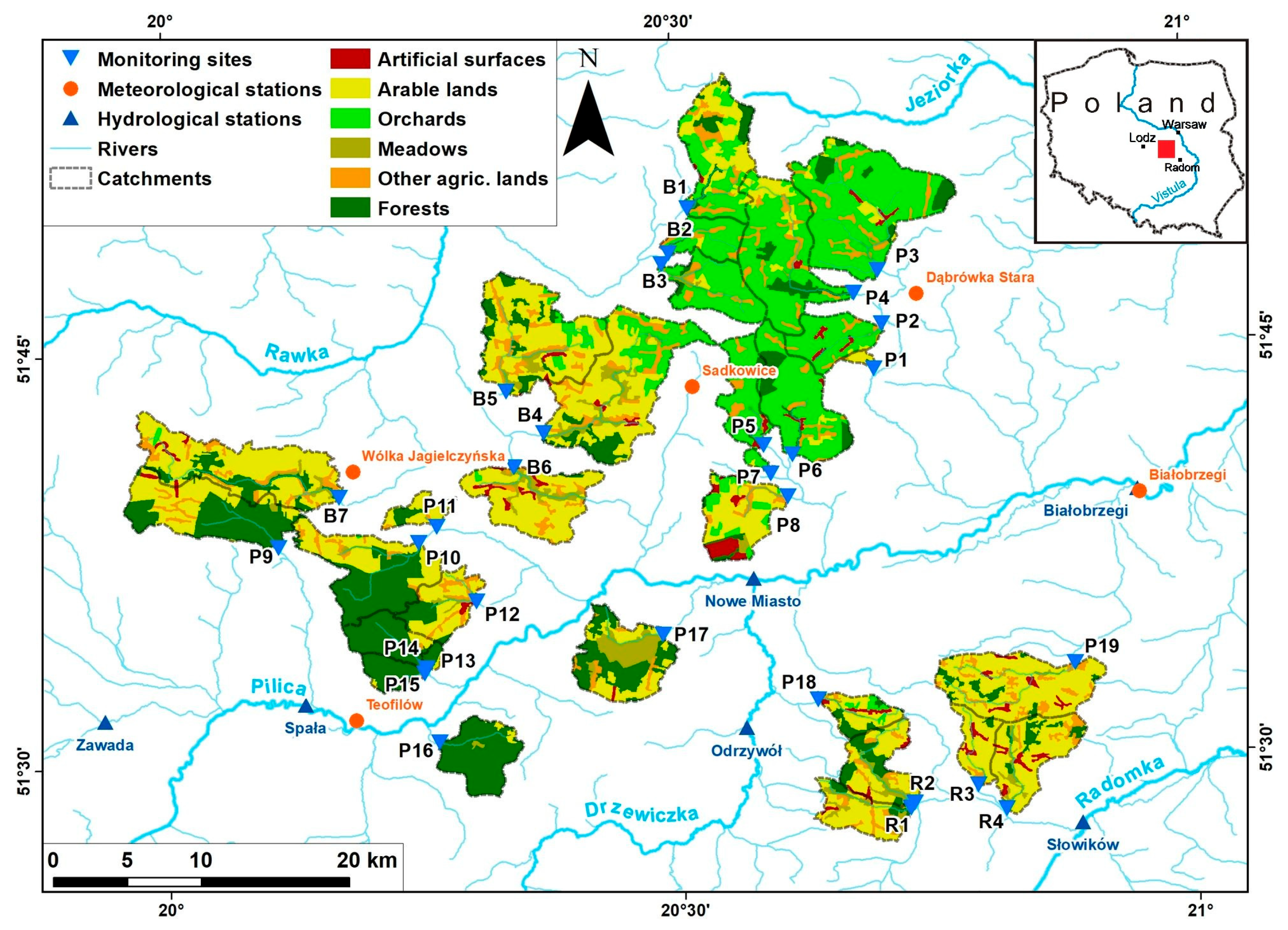
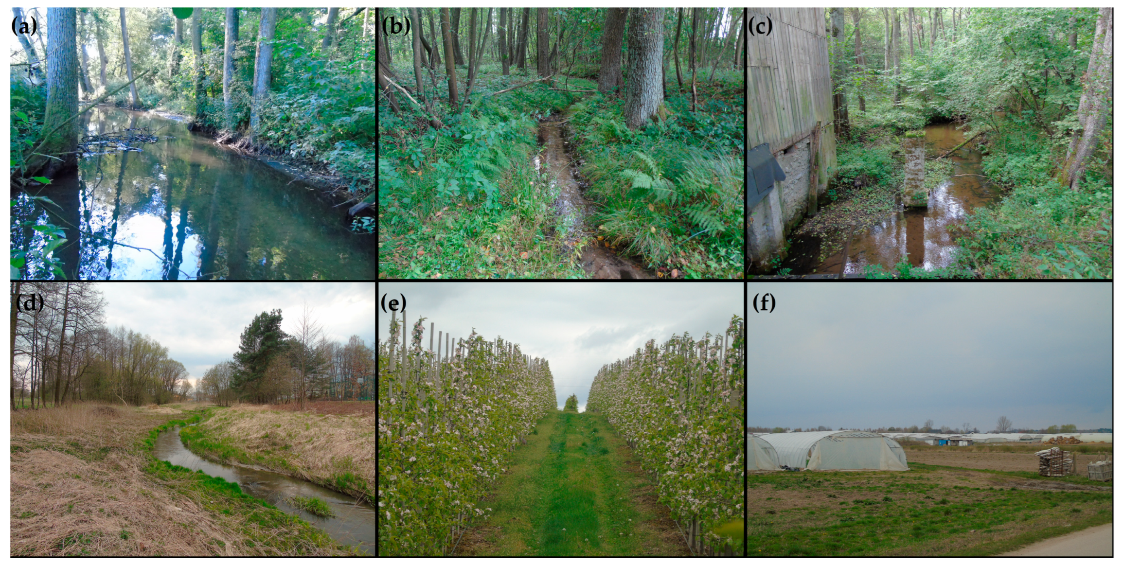
2. Study Area
3. Materials and Methods
3.1. Field and Laboratory Investigations
3.2. Land Cover Evaluation
3.3. Statistical Analysis
4. Results
4.1. Hydrometeorological Background
4.2. Land Cover Classification
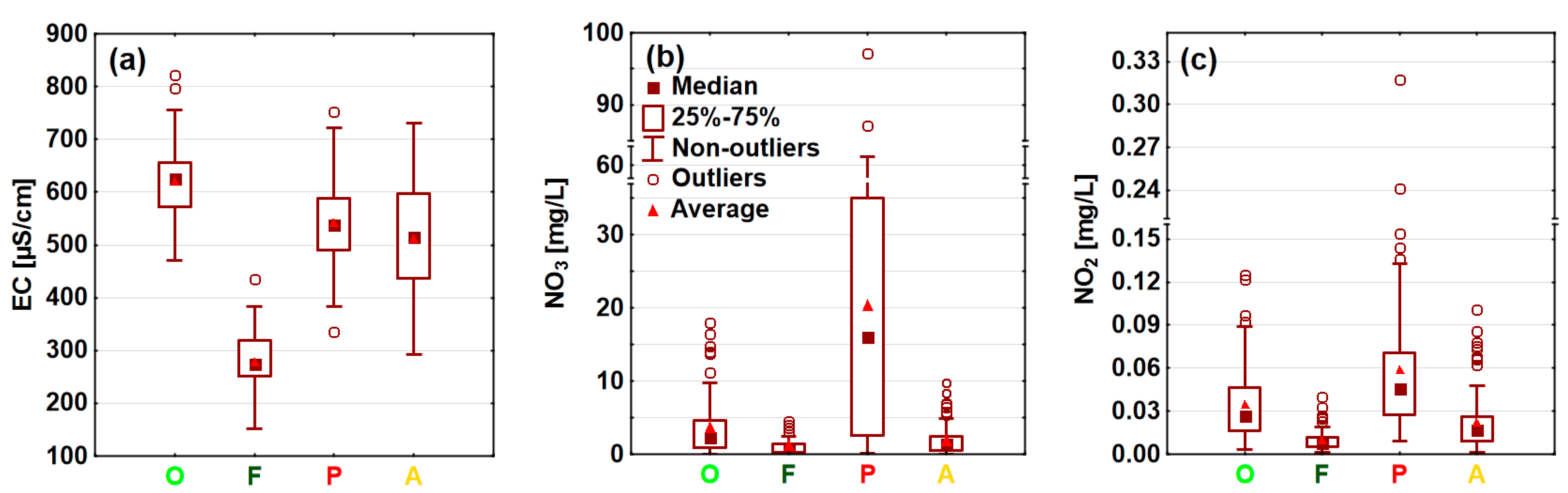
4.3. Spatial Variability of the Water Quality Parameters
4.4. Relationships between Land Use and Water Quality
5. Discussion
5.1. Spatial Variability Evaluation
5.2. The Role of Spatial Scale for Water Quality
5.3. Recommendations and Limitations
Author Contributions
Funding
Data Availability Statement
Acknowledgments
Conflicts of Interest
Appendix A

| Site | River (Alternative Name in Brackets) | Surface Water Body (Name and European Code) | Geographical Coordinates (WGS 84) | A [km2] | Land Use/Land Cover Type Share—Data from CLC 2018 [%] | |||||
|---|---|---|---|---|---|---|---|---|---|---|
| AS | AL | O | M | TAL | F | |||||
| B1 | Białka | Białka PLRW200010272669 | 51.834625 N 20.514992 E | 34.9 | 0.5 | 35.3 | 38.5 | 0 | 85.8 | 13.6 |
| B2 | Stanisławów Stream | 51.807655 N 20.495808 E | 12.1 | 0 | 2.2 | 83.8 | 0 | 97.7 | 2.3 | |
| B3 | Chodnów Stream | 51.801074 N 20.488062 E | 20.2 | 0 | 2.9 | 77.5 | 7 | 96.1 | 3.9 | |
| B4 | Rylka | Rylka PLRW200010272649 | 51.700008 N 20.370354 E | 57.2 | 1.3 | 49 | 19.7 | 9.8 | 89.2 | 9.5 |
| B5 | Regnów Stream (Ossowice-Regnów Canal) | 51.725096 N 20.333412 E | 47.7 | 1.2 | 59 | 7.9 | 4.9 | 84.7 | 14.1 | |
| B6 | Strzałki Stream (Grabice Canal) | 51.679680 N 20.340846 E | 30.5 | 5.3 | 71.2 | 0.9 | 12.8 | 93.6 | 1.1 | |
| B7 | Krzemionka | Rawka to Krzemionka PLRW2000102726199 | 51.663103 N 20.168514 E | 45 | 1.9 | 65.7 | 0.9 | 2.8 | 80.8 | 17.3 |
| P1 | Dańków Stream | Mogielanka PLRW200010254929 | 51.735027 N 20.694095 E | 1.5 | 0 | 77.3 | 3.8 | 0 | 88.8 | 11.2 |
| P2 | Huta Błędowska Stream | 51.762066 N 20.702355 E | 16.4 | 5.5 | 2 | 84.6 | 0 | 94.5 | 0 | |
| P3 | Ciechlin Stream (Machnatka) | 51.794843 N 20.700564 E | 61 | 1.3 | 3.8 | 76.7 | 1.6 | 90.5 | 8.2 | |
| P4 | Mogielanka | 51.781233 N 20.676230 E | 44.5 | 0.6 | 10.9 | 67.5 | 2.6 | 90.1 | 9.3 | |
| P5 | Trębaczew Stream | Gostomka PLRW2000102549149 | 51.690339 N 20.584836 E | 17.4 | 2.9 | 0 | 78.1 | 1.9 | 90.9 | 6.2 |
| P6 | Gostomka (Żelazna) | 51.684113 N 20.612259 E | 33.5 | 1.4 | 2.9 | 73.7 | 0 | 84 | 14.6 | |
| P7 | Władysławów Stream | 51.673083 N 20.591273 E | 1.7 | 0 | 15.5 | 84.5 | 0 | 100 | 0 | |
| P8 | Rosocha Stream | 51.658828 N 20.607247 E | 23.4 | 13.9 | 50.5 | 19 | 2.6 | 80.8 | 5.3 | |
| P9 | Gać | Gać PLRW200010254729 | 51.632941 N 20.109243 E | 36.7 | 1.3 | 38.2 | 0 | 0.7 | 43.5 | 55.2 |
| P10 | Luboczanka | Luboczanka (Lubocz) PLRW200010254769 | 51.634699 N 20.246401 E | 36.5 | 0.2 | 37.7 | 0.2 | 1.2 | 44.3 | 55.5 |
| P11 | Kanice Nowe Stream | 51.644287 N 20.264033 E | 6.8 | 0.4 | 72.7 | 0 | 0 | 78.9 | 20.7 | |
| P12 | Rzeczyca | 51.598556 N 20.301362 E | 16.7 | 2.4 | 54.1 | 0 | 5.9 | 76.3 | 21.3 | |
| P13 | Liciążna Stream (E) | Olszówka PLRW2000102547569 | 51.558735 N 20.252704 E | 1.8 | 0 | 19.5 | 0 | 0 | 19.5 | 80.5 |
| P14 | Olszówka (Struga) | 51.558061 N 20.251921 E | 13.5 | 0 | 8.2 | 0 | 0 | 11.6 | 88.4 | |
| P15 | Liciążna Stream (W) | 51.555406 N 20.250376 E | 7.3 | 0 | 2 | 0 | 0 | 5.1 | 94.9 | |
| P16 | Ceteń Stream (Cetenka) | Ceteń Stream PLRW2000102547529 | 51.513607 N 20.263300 E | 19.8 | 0 | 3.4 | 0 | 1.4 | 4.8 | 95.2 |
| P17 | Kiełcznica | Kiełcznica PLRW200015254792 | 51.576481 N 20.484243 E | 30.2 | 0.7 | 26.3 | 0 | 24.1 | 56.4 | 42.9 |
| P18 | Kozieniec Stream | Kozieniec Stream PLRW200010254889 | 51.535054 N 20.633020 E | 10.5 | 7.9 | 52.1 | 12.8 | 4.8 | 72.2 | 19.9 |
| P19 | Pierzchnianka | Pierzchnianka PLRW200010254949 | 51.554206 N 20.884437 E | 39.4 | 4.3 | 74.5 | 0 | 0.9 | 88 | 7.7 |
| R1 | Przystałowice Duże Stream | Wiązownica PLRW200010252499 | 51.468265 N 20.721298 E | 15.2 | 2.7 | 58.5 | 0 | 16.1 | 87.8 | 9.5 |
| R2 | Potworów Stream | 51.471326 N 20.724903 E | 19.6 | 3.3 | 51.6 | 0 | 12.6 | 73.7 | 23 | |
| R3 | Grabowska Wola Stream | 51.481252 N 20.787154 E | 10.4 | 8.9 | 80.3 | 0 | 3.2 | 88 | 3.1 | |
| R4 | Wrzeszczów Stream | 51.466403 N 20.814512 E | 24.4 | 5.9 | 65.8 | 0 | 8.2 | 81.8 | 12.3 | |
Appendix B
| Parameter | H | Χ2 | df | Median | p-Level | Catchment Groups | ||||
|---|---|---|---|---|---|---|---|---|---|---|
| O | F | P | A | |||||||
| EC | 223.92 | 165.06 | 3 | 531.50 | 0.00 | O | ||||
| F | ||||||||||
| P | ||||||||||
| A | ||||||||||
| NO3 | 115.56 | 76.45 | 3 | 1.62 | 0.00 | O | ||||
| F | ||||||||||
| P | ||||||||||
| A | ||||||||||
| NO2 | 141.09 | 98.89 | 3 | 0.02 | 0.00 | O | ||||
| F | ||||||||||
| P | ||||||||||
| A | ||||||||||
| NH4 | 9.75 | 6.82 | 3 | 0.23 | 0.078 | O | ||||
| F | ||||||||||
| P | ||||||||||
| A | ||||||||||
| Ca | 107.98 | 107.23 | 3 | 66.85 | 0.00 | O | ||||
| F | ||||||||||
| P | ||||||||||
| A | ||||||||||
| Mg | 183.50 | 134.81 | 3 | 10.40 | 0.00 | O | ||||
| F | ||||||||||
| P | ||||||||||
| A | ||||||||||
| K | 157.00 | 113.40 | 3 | 2.38 | 0.00 | O | ||||
| F | ||||||||||
| P | ||||||||||
| A | ||||||||||
| Na | 129.93 | 105.31 | 3 | 6.68 | 0.00 | O | ||||
| F | ||||||||||
| P | ||||||||||
| A | ||||||||||
| As | 36.27 | 26.55 | 3 | 0.06 | 0.00 | O | ||||
| F | ||||||||||
| P | ||||||||||
| A | ||||||||||
| Ba | 64.27 | 49.62 | 3 | 0.02 | 0.00 | O | ||||
| F | ||||||||||
| P | ||||||||||
| A | ||||||||||
| Sr | 83.05 | 81.08 | 3 | 0.10 | 0.00 | O | ||||
| F | ||||||||||
| P | ||||||||||
| A | ||||||||||
| V | 167.57 | 124.63 | 3 | 0.04 | 0.00 | O | ||||
| F | ||||||||||
| P | ||||||||||
| A | ||||||||||
References
- Afroz, R.; Masud, M.M.; Akhtar, R.; Duasa, J.B. Water pollution: Challenges and future direction for water resource management policies in Malaysia. Environ. Urban. ASIA 2014, 5, 63–81. [Google Scholar] [CrossRef]
- Han, D.; Currell, M.; Cao, G. Deep challenges for China’s war on water pollution. Environ. Pollut. 2016, 218, 1222–1233. [Google Scholar] [CrossRef] [PubMed]
- Khatri, N.; Tyagi, S. Influences of natural and anthropogenic factors on surface and groundwater quality in rural and urban areas. Front. Life Sci. 2014, 8, 23–39. [Google Scholar] [CrossRef]
- Akhtar, N.; Syakir Ishak, M.I.; Bhawani, S.A.; Umar, K. Various Natural and Anthropogenic Factors Responsible for Water Quality Degradation: A Review. Water 2021, 13, 2660. [Google Scholar] [CrossRef]
- Campling, P.; Joris, I.; Calliera, M.; Capri, E.; Marchis, A.; Kuczynska, A.; Vereijken, T.; Majewska, Z.; Belmans, E.; Borremans, L.; et al. A multiactor, participatory approach to identify policy and technical barriers to better farming practicies that protect our drinking wáter sources. Sci. Total Environ. 2021, 755, 142971. [Google Scholar] [CrossRef]
- Shukla, S.; Saxena, A. Sources and Leaching of Nitrate Contamination in Groundwater. Curr. Sci. 2020, 118, 883–891. [Google Scholar] [CrossRef]
- Preisner, M.; Smol, M.; Szołdrowska, D. Trends, insights and effects of the Urban Wastewater Treatment Directive (91/271/EEC) implementation in the light of the Polish coastal zone eutrophication. Environ. Manag. 2021, 67, 342–354. [Google Scholar] [CrossRef] [PubMed]
- Poikane, S.; Kelly, M.G.; Várbíró, G.; Borics, G.; Erős, T.; Hellsten, S.; Kolada, A.; Lukács, B.A.; Solheim, A.L.; López, J.P.; et al. Estimating nutrient thresholds for eutrophication management: Novel insights from understudied lake types. Sci. Total Environ. 2022, 827, 154242. [Google Scholar] [CrossRef]
- Andersen, J.H.; Carstensen, J.; Conley, D.J.; Dromph, K.; Fleming-Lehtinen, V.; Gustafsson, B.G.; Josefson, A.B.; Norkko, A.; Villnäs, A.; Murray, C. Long-Term Temporal and Spatial Trends in Eutrophication Status of the Baltic Sea. Biol. Rev. 2017, 92, 135–149. [Google Scholar] [CrossRef]
- Murray, C.J.; Muller-Karulis, B.; Carstensen, J.; Conley, D.J.; Gustafsson, B.G.; Andersen, J.H. Past, Present and Future Eutrophication Status of the Baltic Sea. Front. Mar. Sci. 2019, 6, 2. [Google Scholar] [CrossRef]
- Rönnberg, C.; Bonsdorff, E. Baltic Sea eutrophication: Area-specific ecological consequences. Hydrobiologia 2004, 514, 227–241. [Google Scholar] [CrossRef]
- Savchuk, O.P. Large-Scale Nutrient Dynamics in the Baltic Sea, 1970–2016. Front. Mar. Sci. 2018, 5, 5. [Google Scholar] [CrossRef]
- EUR-Lex Council Directive 91/676/EEC of 12 December 1991 Concerning the Protection of Waters against Pollution Caused by Nitrates from Agricultural Sources. Off. J. Eur. Communities 1991, 375, 1–8. Available online: https://eur-lex.europa.eu/LexUriServ/LexUriServ.do?uri=CELEX:31991L0676:EN:HTML (accessed on 19 November 2023).
- Van Grinsven, H.J.M.; Tiktak, A.; Rougoor, C.W. Evaluation of the Dutch implementation of the nitrates directive, the water framework directive and the national emission ceilings directive. NJAS-Wagening. J. Life Sci. 2016, 78, 69–84. [Google Scholar] [CrossRef]
- Smith, R.J.N.; Glegg, G.A.; Parkinson, R.; Richards, J.P. Evaluating the implementation of the Nitrates Directive in Denmark and England using an actor-orientated approach. Eur. Environ. 2007, 17, 124–144. [Google Scholar] [CrossRef]
- Musacchio, A.; Re, V.; Mas-Pla, J.; Sacchi, E. EU Nitrates Directive, from theory to practice: Environmental effectiveness and influence of regional governance on its performance. Ambio 2020, 49, 504–516. [Google Scholar] [CrossRef]
- Soro, M.-P.; N’goran, K.M.; Ouattara, A.A.; Yao, K.M.; Kouassi, N.L.B.; Diaco, T. Nitrogen and phosphorus spatio-temporal distribution and fluxes intensifying eutrophication in three tropical rivers of Côte d’Ivoire (West Africa). Mar. Pollut. Bull. 2023, 186, 114391. [Google Scholar] [CrossRef]
- Richards, S.; Paterson, E.; Withers, P.J.; Stutter, M. Septic tank discharges as multi-pollutant hotspots in catchments. Sci. Total Environ. 2016, 542, 854–863. [Google Scholar] [CrossRef]
- Pouye, A.; Cissé Faye, S.; Diédhiou, M.; Gaye, C.B.; Taylor, R.G. Nitrate contamination of urban groundwater and heavy rainfall: Observations from Dakar, Senegal. Vadose Zone J. 2023, 22, e20239. [Google Scholar] [CrossRef]
- Piasecki, A. Water and Sewage Management Issues in Rural Poland. Water 2019, 11, 625. [Google Scholar] [CrossRef]
- Ławniczak, A.E.; Zbierska, J.; Nowak, B.; Achtenberg, K.; Grześkowiak, A.; Kanas, K. Impact of agriculture and land use on nitrate contamination in groundwater and running waters in central-west Poland. Environ. Monit. Assess. 2016, 188, 172. [Google Scholar] [CrossRef] [PubMed]
- Jiang, R.; Hatano, R.; Zhao, Y.; Woli, K.P.; Kuramochi, K.; Shimizu, M.; Hayakawa, A. Factors controlling nitrogen and dissolved organic carbon exports across timescales in two watersheds with different land uses. Hydrol. Process. 2014, 28, 5105–5121. [Google Scholar] [CrossRef]
- Mortvedt, J.J. Heavy metal contaminants in inorganic and organic fertilizers. Fert. Res. 1995, 43, 55–61. [Google Scholar] [CrossRef]
- Alengebawy, A.; Abdelkhalek, S.T.; Qureshi, S.R.; Wang, M.-Q. Heavy Metals and Pesticides Toxicity in Agricultural Soil and Plants: Ecological Risks and Human Health Implications. Toxics 2021, 9, 42. [Google Scholar] [CrossRef] [PubMed]
- Gimeno-García, E.; Andreu, V.; Boluda, R. Heavy metals incidence in the application of inorganic fertilizers and pesticides to rice farming soils. Environ. Pollut. 1996, 92, 19–25. [Google Scholar] [CrossRef]
- Syafrudin, M.; Kristanti, R.A.; Yuniarto, A.; Hadibarata, T.; Rhee, J.; Al-onazi, W.A.; Algarni, T.S.; Almarri, A.H.; Al-Mohaimeed, A.M. Pesticides in Drinking Water—A Review. Int. J. Environ. Res. Public Health 2021, 18, 468. [Google Scholar] [CrossRef]
- Staponites, L.R.; Barták, V.; Bílý, M.; Simon, O.P. Performance of landscape composition metrics for predicting water quality in headwater catchments. Sci. Rep. 2019, 9, 14405. [Google Scholar] [CrossRef]
- Gelsey, K.; Chang, H.; Ramirez, D. Effects of landscape characteristics, anthropogenic factors, and seasonality on water quality in Portland, Oregon. Environ. Monit. Assess. 2023, 195, 219. [Google Scholar] [CrossRef]
- Yang, H.; Kong, J.; Hu, H.; Du, Y.; Gao, M.; Chen, F. A Review of Remote Sensing for Water Quality Retrieval: Progress and Challenges. Remote Sens. 2022, 14, 1770. [Google Scholar] [CrossRef]
- Hajigholizadeh, M.; Moncada, A.; Kent, S.; Melesse, A.M. Land–Lake Linkage and Remote Sensing Application in Water Quality Monitoring in Lake Okeechobee, Florida, USA. Land 2021, 10, 147. [Google Scholar] [CrossRef]
- Niu, C.; Tan, K.; Jia, X.; Wang, X. Deep learning based regression for optically inactive inland water quality parameter esti-mation using airborne hyperspectral imagery. Environ. Pollut. 2021, 286, 117534. [Google Scholar] [CrossRef]
- Matysik, M.; Absalon, D.; Ruman, M. Surface water quality in relation to land cover in agricultural catchments (Liswarta river basin case study). Pol. J. Environ. Stud. 2015, 24, 175–184. [Google Scholar] [CrossRef] [PubMed]
- Lei, C.; Wagner, P.D.; Fohrer, N. Effects of land cover, topography, and soil on stream water quality at multiple spatial and seasonal scales in a German lowland catchment. Ecol. Indic. 2021, 120, 106940. [Google Scholar] [CrossRef]
- Xu, S.; Li, S.; Zhong, J.; Li, C. Spatial Scale Effects of the Variable Relationships between Landscape Pattern and Water Quality: Example from an Agricultural Karst River Basin, Southwestern China. Agric. Ecosyst. Environ. 2020, 300, 106999. [Google Scholar] [CrossRef]
- Pak, H.; Chuah, C.; Yong, E.; Snyder, S. Effects of land use configuration, seasonality and point source on water quality in a tropical watershed: A case study of the Johor River Basin. Sci. Total Environ. 2021, 780, 146661. [Google Scholar] [CrossRef] [PubMed]
- Tahiru, A.A.; Doke, D.A.; Baatuuwie, B.N. Effect of land use and land cover changes on water quality in the Nawuni Catchment of the White Volta Basin, Northern Region, Ghana. Appl. Water Sci. 2020, 10, 198. [Google Scholar] [CrossRef]
- Łaszewski, M.; Fedorczyk, M.; Gołaszewska, S.; Kieliszek, Z.; Maciejewska, P.; Miksa, J.; Zacharkiewicz, W. Land Cover Effects on Selected Nutrient Compounds in Small Lowland Agricultural Catchments. Land 2021, 10, 182. [Google Scholar] [CrossRef]
- Poor, C.J.; McDonnell, J.J. The effects of land use on stream nitrate dynamics. J. Hydrol. 2007, 332, 54–68. [Google Scholar] [CrossRef]
- Żelazny, M.; Siwek, J. Determinants of Seasonal Changes in Streamwater Chemistry in Small Catchments with Different Land Use: Case Study from Poland’s Carpathian Foothills. Pol. J. Environ. Stud. 2012, 21, 791–804. [Google Scholar]
- Camara, M.; Jamil, N.R.; Bin Abdullah, A.F. Impact of Land Uses on Water Quality in Malaysia: A Review. Ecol. Process. 2019, 8, 10. [Google Scholar] [CrossRef]
- Solon, J.; Borzyszkowski, J.; Bidłasik, M.; Richling, A.; Badora, K.; Balon, J.; Brzezińska-Wójcik, T.; Chabudziński, Ł.; Dobrowolski, R.; Grzegorczyk, I.; et al. Physico-geographical mesoregions of Poland: Verification and adjustment of boundaries on the basis of contemporary spatial data. Geogr. Pol. 2018, 91, 143–170. [Google Scholar] [CrossRef]
- Makowska, A. Mapa Geologiczna Polski 1:200,000, Arkusz: Skierniewice; Państwowy Instytut Geologiczny: Warsaw, Poland, 1970. Available online: https://bazadata.pgi.gov.pl/data/mgp200/mapy/edycja1/mgp200A49-edycja1.jpg (accessed on 19 November 2023).
- Beck, H.E.; Zimmermann, N.E.; McVicar, T.R.; Vergopolan, N.; Berg, A.; Wood, E.F. Present and future Köppen-Geiger climate classification maps at 1-km resolution. Sci. Data 2018, 5, 180214. [Google Scholar] [CrossRef] [PubMed]
- Piniewski, M. Classification of natural flow regimes in Poland. River Res. Appl. 2017, 33, 1205–1218. [Google Scholar] [CrossRef]
- Główny Inspektorat Ochrony Środowiska (Chief Inspectorate of Environmental Protection). Ocena Stanu Jednolitych Części wód rzek i Zbiorników Zaporowych w Latach 2016–2021 na Podstawie Monitoringu. Available online: https://wody.gios.gov.pl/pjwp/api/publications/media/782 (accessed on 19 November 2023).
- Kulikowski, R. Ogrodnictwo w Polsce. Rozmieszczenie, struktura upraw i rola w produkcji rolniczej. Przegląd Geogr. 2007, 79, 79–98. [Google Scholar]
- Wójcik, M.; Traczyk, A. Changes in the Spatial Organisation of Fruit Growing at the Beginning of the 21St Century: The Case of Grójec Poviat (Mazovia Voivodeship, Poland). Quaest. Geogr. 2017, 36, 71–84. [Google Scholar] [CrossRef][Green Version]
- Lenart-Boroń, A.; Wolanin, A.; Jelonkiewicz, E.; Żelazny, M. The effect of anthropogenic pressure shown by microbiological and chemical water quality indicators on the main rivers of Podhale, southern Poland. Environ. Sci. Pollut. Res. 2017, 24, 12938–12948. [Google Scholar] [CrossRef]
- Jandová, V.; Bucková, M.; Hegrová, J.; Dostál, I.; Huzlík, J.; Effenberger, K.; Ličbinský, R. The Relationship among Precipitation, Application of Salt in Winter Road Maintenance and the Quality of Waterways and Soil around Motorway. Water 2020, 12, 2206. [Google Scholar] [CrossRef]
- Lachhab, A.; Trent, M.M.; Motsko, J. Multimetric approach in the effects of small impoundments on stream water quality: Case study of Faylor and Walker Lakes on Middle Creek, Snyder County, PA. Water Environ. J. 2021, 35, 1007–1017. [Google Scholar] [CrossRef]
- Stępniewski, K.; Łaszewski, M. Spatial and Seasonal Dynamics of Inorganic Nitrogen and Phosphorous Compounds in an Orchard-Dominated Catchment with Anthropogenic Impacts. Sustainability 2021, 13, 11337. [Google Scholar] [CrossRef]
- Moss, B. Water Pollution by Agriculture. Philos. Trans. R. Soc. B Biol. Sci. 2008, 363, 659–666. [Google Scholar] [CrossRef]
- Jiang, Y.; Xie, Z.; Zhang, H.; Xie, H.; Cao, Y. Effects of land use types on dissolved trace metal concentrations in the Le’an River Basin, China. Environ. Monit. Assess. 2017, 189, 633. [Google Scholar] [CrossRef] [PubMed]
- Andersen, C.B.; Lewis, G.P.; Sargent, K.A. Influence of wastewater-treatment effluent on concentrations and fluxes of solutes in the Bush River, South Carolina, during extreme drought conditions. Environ. Geosci. 2004, 11, 28–41. [Google Scholar] [CrossRef]
- Figueroa-Nieves, D.; McDowell, W.H.; Potter, J.D.; Martínez, G.; Ortiz-Zayas, J.R. Effects of sewage effluents on water quality in tropical streams. J. Environ. Qual. 2014, 43, 2053–2063. [Google Scholar] [CrossRef] [PubMed]
- Rosina, K.; Batista e Silva, F.; Vizcaino, P.; Herrera, M.M.; Freire, S.; Schiavina, M. Increasing the detail of European land use/cover data by combining heterogeneous data sets. Int. J. Digit. Earth 2018, 13, 602–626. [Google Scholar] [CrossRef]
- Popovici, E.A.; Bălteanu, D.; Kucsicsa, G. Assessment of changes in land-use and land-cover pattern in Romania using CORINE Land Cover Database. Carpathian J. Earth Environ. Sci. 2013, 8, 195–208. [Google Scholar]
- Śleszyński, P.; Gibas, P.; Sudra, P. The Problem of Mismatch between the CORINE Land Cover Data Classification and the Development of Settlement in Poland. Remote Sens. 2020, 12, 2253. [Google Scholar] [CrossRef]
- Kändler, M.; Blechinger, K.; Seidler, C.; Pavlů, V.; Šanda, M.; Dostál, T.; Krása, J.; Vitvar, T.; Štich, M. Impact of land use on water quality in the upper Nisa catchment in the Czech Republic and in Germany. Sci. Total Environ. 2017, 586, 1316–1325. [Google Scholar] [CrossRef]
- Gutry-Korycka, M.; Woronko, D.; Suchożebrski, J. Uwarunkowanie regionalne maksymalnych prawdopodobnych przepływów rzek polskich. Prace Stud. Geogr. 2009, 43, 25–48. [Google Scholar]
- Żelazny, M. Czasowo-Przestrzenna Zmienność cech Fizykochemicznych wód Tatrzańskiego Parku Narodowego; Instytut Geografii i Gospodarki Przestrzennej Uniwersytetu Jagiellońskiego: Kraków, Poland, 2012. [Google Scholar]
- Miranda, L.S.; Deilami, K.; Ayoko, G.A.; Egodawatta, P.; Goonetilleke, A. Influence of land use class and configuration on water-sediment partitioning of heavy metals. Sci. Total Environ. 2022, 804, 150116. [Google Scholar] [CrossRef]
- Havlíková, P.; Mrkva, L.; Chuman, T.; Janský, B. Surface water quality in the rural catchment of the Šlapanka River, Czechia: Change over time. Environ. Earth Sci. 2023, 82, 379. [Google Scholar] [CrossRef]
- Mori, G.B.; Paula, F.R.; Ferraz, S.F.B.; Camargo, A.F.M.; Martinelli, L.F. Influence of landscape properties on stream water quality in agricultural catchments in Southeastern Brazil. Ann. Limnol.-Inter. J. Lim. 2015, 51, 11–21. [Google Scholar] [CrossRef]
- Kaiser, H.F. An index of factorial simplicity. Psychometrika 1974, 39, 31–36. [Google Scholar] [CrossRef]
- Żelazny, M.; Rajwa-Kuligiewicz, A.; Bojarczuk, A.; Pęksa, Ł. Water temperature fluctuation patterns in surface waters of the Tatra Mts., Poland. J. Hydrol. 2018, 564, 824–835. [Google Scholar] [CrossRef]
- de Mello, K.D.; Valente, R.A.; Randhir, T.O.; Vettorazzi, C.A. Impacts of tropical forest cover on water quality in agricultural watersheds in southeastern Brazil. Ecol. Indic. 2018, 93, 1293–1301. [Google Scholar] [CrossRef]
- Peng, S.; Li, S. Scale relationship between landscape pattern and water quality in different pollution source areas: A case study of the Fuxian Lake watershed, China. Ecol. Indic. 2021, 121, 107136. [Google Scholar] [CrossRef]
- White, S.A.; Santos, I.R.; Hessey, S. Nitrate loads in sub-tropical headwater streams driven by intensive horticulture. Environ. Pollut. 2018, 243, 1036–1046. [Google Scholar] [CrossRef]
- Sowiński, P. Variability of the content of macroelements in soils of a young glacial river valley-A geochemical landscape approach. J. Elem. 2016, 21, 1343–1358. [Google Scholar] [CrossRef]
- Cappuyns, V.; Slabbinck, E. Occurrence of Vanadium in Belgian and European Alluvial Soils. Appl. Environ. Soil Sci. 2012, 2012, 979501. [Google Scholar] [CrossRef]
- Smedley, P.L.; Kinniburgh, D. Arsenic in Groundwater and the Environment. In Essentials of Medical Geology; Selinus, O., Ed.; Springer: Dordrecht, The Netherlands, 2013; pp. 279–310. [Google Scholar] [CrossRef]
- Musgrove, M. The occurrence and distribution of strontium in U.S. groundwater. Appl. Geochem. 2021, 126, 104867. [Google Scholar] [CrossRef]
- Traaen, T.S.; Frogner, T.; Hindar, A.; Kleiven, E.; Lande, A.; Wright, R.F. Whole-catchment liming at Tjønnstrond, Norway: An 11-year record. Water Air Soil Pollut. 1997, 94, 163–180. [Google Scholar] [CrossRef]
- Orzepowski, W.; Pulikowski, K. Magnesium, calcium, potassium and sodium content in groundwater and surface water in arable lands in the commune of Kąty Wrocławskie. J. Elementol. 2008, 13, 605–614. [Google Scholar]
- Hamilton, P.A.; Helsel, D.R. Effects of agriculture on ground-water quality in five regions of the United States. Groundwater 2010, 33, 217–226. [Google Scholar] [CrossRef]
- Simon, L. Potentially harmful elements in agricultural soils. In PHEs, Environment and Human Health: Potentially Harmful Elements in the Environment and the Impact on Human Health; Springer: Berlin/Heidelberg, Germany, 2014; pp. 85–150. [Google Scholar] [CrossRef]
- Sun, J.; Zhao, Q.; Wang, S.; Wang, J.; Li, Z.; Liu, X. Chemical behaviours of Arsenium, Chromium, Mercury, Lead, and Strontium in aqueous system. E3S Web Conf. 2021, 290, 01022. [Google Scholar] [CrossRef]
- Simon, S.; Brun, L.; Guinaudeau, J.; Sauphanor, B. Pesticide use in current and innovative apple orchard systems. Agron. Sustain. Dev. 2011, 31, 541–555. [Google Scholar] [CrossRef]
- Wieczorek, K.; Turek, A.; Wolf, W.M. Combined Effect of Climate and Anthropopressure on River Water Quality. Int. J. Environ. Res. Public Health 2023, 20, 3032. [Google Scholar] [CrossRef]
- Ahlgren, J.; Djodjic, F.; Wallin, M. Barium as a potential indicator of phosphorus in agricultural runoff. J. Environ. Qual. 2012, 41, 208–216. [Google Scholar] [CrossRef]
- Kuczyńska, A.; Jarnuszewski, G.; Nowakowska, M.; Wexler, S.K.; Wiśniowski, Z.; Burczyk, P.; Durkowski, T.; Woźnicka, M. Identifying causes of poor water quality in a Polish agricultural catchment for designing effective and targeted mitigation measures. Sci. Total Environ. 2021, 765, 144125. [Google Scholar] [CrossRef]
- Bawiec, A.; Kajewska-Szkudlarek, J.; Pulikowski, K.; Pawęska, K. Assessment of the Validity of Introducing Nitrate Vulnerable Zones in Large Areas. Sustainability 2022, 14, 6585. [Google Scholar] [CrossRef]
- Ilnicki, P. Polskie Rolnictwo a Ochrona Środowiska; Wyd. AR: Poznań, Poland, 2004. [Google Scholar]
- Anyszka, Z.; Rogowska, M.; Stępowska, A.; Ślusarski, C.; Wrzodak, R. Metodyka Integrowanej Ochrony Papryki; Instytut Ogrodnictwa: Skierniewice, Poland, 2013; Available online: https://www.inhort.pl/files/sor/metodyki_ior/Metodyka_int_ochrony_papryki_doradcy.pdf (accessed on 19 November 2023).
- Kowalczyk, W.; Wrona, D.; Przybyłko, S. Effect of Nitrogen Fertilization of Apple Orchard on Soil Mineral Nitrogen Content, Yielding of the Apple Trees and Nutritional Status of Leaves and Fruits. Agriculture 2022, 12, 2169. [Google Scholar] [CrossRef]
- Clune, J.W.; Crawford, J.K.; Chappell, W.T.; Boyer, E.W. Differential effects of land use on nutrient concentrations in streams of Pennsylvania. Environ. Res. Commun. 2020, 2, 115003. [Google Scholar] [CrossRef]
- Fernandes, A.C.P.; Martins, L.M.D.O.; Fernandes, L.F.S.; Cortes, R.M.V.; Pacheco, F.A.L. Effect of landscape metrics on water quality over three decades: A case study of the Ave River basin, Portugal. WIT Trans. Ecol. Environ. 2020, 242, 39–49. [Google Scholar] [CrossRef]
- Jachniak, E.; Jaguś, A.; Młyniuk, A.; Nycz, B. The quality problems of the dammed water in the mountain forest catchment. J. Ecol. Eng. 2019, 20, 165–171. [Google Scholar] [CrossRef] [PubMed]
- Cánovas, F.M.; Cañas, R.A.; de la Torre, F.N.; Pascual, M.B.; Castro-Rodríguez, V.; Avila, C. Nitrogen metabolism and biomass production in forest trees. Front. Plant Sci. 2018, 9, 1449. [Google Scholar] [CrossRef] [PubMed]
- Ayele, G.T.; Yu, B.; Bruere, A.; Hamilton, D. Response of streamflow and nutrient loads in a small temperate catchment subject to land use change. Environ. Monit. Assess. 2023, 195, 1418. [Google Scholar] [CrossRef]
- Hughes, A.O.; Quinn, J.M. The effect of forestry management activities on stream water quality within a headwater plantation Pinus radiata forest. For. Ecol. Manag. 2019, 439, 41–54. [Google Scholar] [CrossRef]
- Schulz, H.; Härtling, S.; Stange, C.F. Species-specific differences in nitrogen uptake and utilization by six European tree species. J. Plant Nutr. Soil Sci. 2011, 174, 28–37. [Google Scholar] [CrossRef]
- Song, M.; Jiang, Y.; Liu, Q.; Tian, Y.; Liu, Y.; Xu, X.; Kang, M. Catchment versus Riparian Buffers: Which Land Use Spatial Scales Have the Greatest Ability to Explain Water Quality Changes in a Typical Temperate Watershed? Water 2021, 13, 1758. [Google Scholar] [CrossRef]
- Weber, G.; Kubiniok, J. Spring waters as an indicator of nitrate and pesticide pollution of rural watercourses from nonpoint sources: Results of repeated monitoring campaigns since the early 2000s in the low mountain landscape of Saarland, Germany. Environ. Sci. Eur. 2022, 34, 53. [Google Scholar] [CrossRef]
- Przydatek, G. Multi-indicator analysis of the influence of old municipal landfill sites on the aquatic environment: Case study. Environ. Monit. Assess. 2019, 191, 773. [Google Scholar] [CrossRef]
- Dębska, K.; Rutkowska, B.; Szulc, W.; Gozdowski, D. Changes in Selected Water Quality Parameters in the Utrata River as a Function of Catchment Area Land Use. Water 2021, 13, 2989. [Google Scholar] [CrossRef]
- Sardans, J.; Peñuelas, J. Potassium: A neglected nutrient in global change. Glob. Ecol. Biogeogr. 2015, 24, 261–275. [Google Scholar] [CrossRef]
- Skowron, P.; Skowrońska, M.; Bronowicka-Mielniczuk, U.; Filipek, T.; Igras, J.; Kowalczyk-Juśko, A.; Krzepiło, A. Anthropogenic sources of potassium in surface water: The case study of the Bystrzyca river catchment, Poland. Agric. Ecosys. Environ. 2018, 265, 454–460. [Google Scholar] [CrossRef]
- Aalipour, M.; Antczak, E.; Dostál, T.; Amiri, B.J. Influences of Landscape Configuration on River Water Quality. Forests 2022, 13, 222. [Google Scholar] [CrossRef]
- de Mello, K.; Valente, R.A.; Ribeiro, M.P.; Randhir, T. Effects of forest cover pattern on water quality of low-order streams in an agricultural landscape in the Pirapora river basin, Brazil. Environ. Monit. Assess. 2022, 194, 189. [Google Scholar] [CrossRef] [PubMed]
- Nielsen, A.; Trolle, D.; Søndergaard, M.; Lauridsen, T.L.; Bjerring, R.; Olesen, J.E.; Jeppesen, E. Watershed land use effects on lake water quality in Denmark. Ecol. Appl. 2012, 22, 1187–1200. [Google Scholar] [CrossRef] [PubMed]
- Wu, J.; Jin, Y.; Hao, Y.; Lu, J. Identification of the control factors affecting water quality variation at multi-spatial scales in a headwater watershed. Environ. Sci. Pollut. Res. 2021, 28, 11129–11141. [Google Scholar] [CrossRef] [PubMed]
- Bhat, S.U.; Khanday, S.A.; Islam, S.T.; Sabha, I. Understanding the spatiotemporal pollution dynamics of highly fragile montane watersheds of Kashmir Himalaya, India. Environ. Pollut. 2021, 286, 117335. [Google Scholar] [CrossRef]
- Ye, L.; Cai, Q.-H.; Liu, R.-Q.; Cao, M. The influence of topography and land use on water quality of Xiangxi River in Three Gorges Reservoir region. Environ. Geol. 2009, 58, 937–942. [Google Scholar] [CrossRef]
- Burgin, A.J.; Hamilton, S.K. Have we overemphasized the role of denitrification in aquatic ecosystems? A review of nitrate removal pathways. Front. Ecol. Environ. 2007, 5, 89–96. [Google Scholar] [CrossRef]
- Sweeney, B.W.; Newbold, J.D. Streamside Forest Buffer Width Needed to Protect Stream Water Quality, Habitat, and Organisms: A Literature Review. JAWRA J. Am. Water Resour. Assoc. 2014, 50, 560–584. [Google Scholar] [CrossRef]
- Buler, Z. Przygotowanie gleby oraz zakładanie sadu. In Metodyka Integrowanej Ochrony Jabłoni; Sobiczewski, P., Ed.; Instytut Ogrodnictwa: Skierniewice, Poland, 2013; Available online: http://www.inhort.pl/files/FAPA/sadownictwo/Doradca/JABLON-DORADCA%20II%20K%20A.pdf (accessed on 19 November 2023).
- Agricultural Census. Statistics Poland. 2020. Available online: https://bdl.stat.gov.pl/bdl/dane/podgrup/temat (accessed on 19 November 2023).
- Carey, R.O.; Migliaccio, K.W. Contribution of wastewater treatment plant effluents to nutrient dynamics in aquatic systems: A review. Environ. Manag. 2009, 44, 205–217. [Google Scholar] [CrossRef] [PubMed]
- Lintern, A.; Wbb, J.A.; Ryu, D.; Liu, S.; Bende-Michl, U.; Waters, D.; Leahy, P.; Wilson, P.; Western, A.W. Key factors influencing differences in stream water quality across space. WIREs Water 2018, 5, e1260. [Google Scholar] [CrossRef]
- Sadeq, M.; Moe, C.L.; Attarassi, B.; Cherkaoui, I.; ElAouad, R.; Idrissi, L. Drinking water nitrate and prevalence of methemoglobinemia among infants and children aged 1–7 years in Moroccan areas. Int. J. Hyg. Environ. Health 2008, 211, 546–554. [Google Scholar] [CrossRef] [PubMed]
- Szlauer-Łukaszewska, A.; Ławicki, Ł.; Engel, J.; Drewniak, E.; Ciężak, K.; Marchowski, D. Quantifying a mass mortality event in freshwater wildlife within the Lower Odra River: Insights from a large European river. Sci. Total Environ. 2024, 907, 167898. [Google Scholar] [CrossRef] [PubMed]
- Sługocki, Ł.; Czerniawski, R. Water Quality of the Odra (Oder) River before and during the Ecological Disaster in 2022: A Warning to Water Management. Sustainability 2023, 15, 8594. [Google Scholar] [CrossRef]
- Tei, F.; De Neve, S.; de Haan, J.; Kristensen, H.L. Nitrogen management of vegetable crops. Agric. Water Manag. 2020, 240, 106316. [Google Scholar] [CrossRef]
- Bednarek, A.; Szklarek, S.; Zalewski, M. Nitrogen pollution removal from areas of intensive farming—Comparison of various denitrification biotechnologies. Ecohydrol. Hydrobiol. 2014, 14, 132–141. [Google Scholar] [CrossRef]
- Robertson, W.D.; Blowes, D.W.; Ptacek, C.J.; Cherry, J.A. Long-term performance of in situ reactive barriers for nitrate remediation. Groundwater 2000, 38, 689–695. [Google Scholar] [CrossRef]
- Schipper, L.A.; Cameron, S.G.; Warneke, S. Nitrate removal from three different effluents using large-scale denitrification beds. Ecol. Eng. 2010, 36, 1552–1557. [Google Scholar] [CrossRef]
- Streeter, M.T.; Schilling, K.E. Quantifying the effectiveness of a saturated buffer to reduce tile NO3-N concentrations in eastern Iowa. Environ. Monit. Assess. 2021, 193, 500. [Google Scholar] [CrossRef]
- Izydorczyk, K.; Michalska-Hejduk, D.; Jarosiewicz, P.; Bydałek, F.; Frątczak, W. Extensive grasslands as an effective measure for nitrate and phosphate reduction from highly polluted subsurface flow—Case studies from Central Poland. Agric. Water Manage. 2018, 203, 240–250. [Google Scholar] [CrossRef]
- Nakhone, L.N.; Tabatabai, M.A. Nitrogen mineralization of leguminous crops in soils. J. Plant Nutr. Soil Sci.-Z. Fur Pflanzenernahr. Und Bodenkd. 2008, 171, 231–241. [Google Scholar] [CrossRef]
- Lötjönen, S.; Ollikainen, M. Does crop rotation with legumes provide an efficient means to reduce nutrient loads and GHG emissions? Rev. Agric. Food Environ. 2017, 98, 283–312. [Google Scholar] [CrossRef]
- Koropeckyj-Cox, L.; Christianson, R.D.; Yuan, Y. Effectiveness of conservation crop rotation for water pollutant reduction from agricultural areas. Trans. ASABE 2021, 64, 691–704. [Google Scholar] [CrossRef]
- Ben Hassen, T.; El Bilali, H. Impacts of the Russia-Ukraine War on Global Food Security: Towards More Sustainable and Resilient Food Systems? Foods 2022, 11, 2301. [Google Scholar] [CrossRef]
- Górski, J.; Dragon, K.; Kaczmarek, P. Nitrate pollution in the Warta River (Poland) between 1958 and 2016: Trend and causes. Environ. Sci. Pollut. Res. 2019, 26, 2038–2046. [Google Scholar] [CrossRef]
- Pekárová, P.; Pekár, J. The impact of land use on stream water quality in Slovakia. J. Hydrol. 1996, 180, 333–350. [Google Scholar] [CrossRef]
- Langhammer, J. Water Quality Changes in the Elbe River Basin, Czech Republic, in the Context of the Post-Socialist Economic Transition. GeoJournal 2010, 75, 185–198. [Google Scholar] [CrossRef]


| Measured Parameter | PC1 | PC2 |
|---|---|---|
| EC | −0.96 | 0.02 |
| NO3 | −0.51 | −0.83 |
| NO2 | −0.62 | −0.73 |
| NH4 | −0.42 | 0.32 |
| Ca | −0.91 | 0.18 |
| Mg | −0.93 | 0.02 |
| K | −0.85 | −0.14 |
| Na | −0.84 | 0.11 |
| As | −0.77 | 0.42 |
| Ba | −0.78 | 0.15 |
| Sr | −0.80 | 0.11 |
| V | −0.91 | 0.05 |
| Eigenvalue | 7.5 | 1.6 |
| Explained variance [%] | 62.8 | 13.4 |
| Parameter | Land Cover Type | 50 | 100 | 250 | 500 | 1000 | TCA |
|---|---|---|---|---|---|---|---|
| EC | Artificial surfaces | 0.32 | 0.30 | 0.35 | 0.40 | 0.41 | 0.29 |
| Arable lands | 0.00 | 0.00 | 0.01 | −0.01 | −0.09 | −0.11 | |
| Orchards | 0.49 | 0.51 | 0.61 | 0.60 | 0.63 | 0.64 | |
| Forested areas | −0.50 | −0.52 | −0.56 | −0.64 | −0.76 | −0.75 | |
| NO3 | Artificial surfaces | 0.45 | 0.44 | 0.40 | 0.38 | 0.47 | 0.49 |
| Arable lands | 0.55 | 0.53 | 0.56 | 0.44 | 0.36 | 0.31 | |
| Orchards | 0.03 | 0.04 | 0.02 | 0.04 | 0.04 | 0.05 | |
| Forested areas | −0.46 | −0.45 | −0.44 | −0.39 | −0.34 | −0.40 | |
| NO2 | Artificial surfaces | 0.59 | 0.57 | 0.55 | 0.53 | 0.60 | 0.56 |
| Arable lands | 0.39 | 0.38 | 0.43 | 0.32 | 0.23 | 0.15 | |
| Orchards | 0.16 | 0.18 | 0.20 | 0.22 | 0.20 | 0.22 | |
| Forested areas | −0.53 | −0.53 | −0.53 | −0.51 | −0.48 | −0.51 | |
| NH4 | Artificial surfaces | 0.22 | 0.23 | 0.25 | 0.22 | 0.24 | 0.28 |
| Arable lands | −0.30 | −0.31 | −0.29 | −0.31 | −0.33 | −0.31 | |
| Orchards | 0.20 | 0.22 | 0.26 | 0.28 | 0.20 | 0.21 | |
| Forested areas | −0.14 | −0.16 | −0.19 | −0.21 | −0.25 | −0.15 | |
| Ca | Artificial surfaces | 0.23 | 0.24 | 0.30 | 0.36 | 0.37 | 0.22 |
| Arable lands | 0.03 | 0.04 | 0.07 | 0.09 | 0.03 | 0.01 | |
| Orchards | 0.44 | 0.45 | 0.55 | 0.53 | 0.57 | 0.58 | |
| Forested areas | −0.52 | −0.54 | −0.58 | −0.67 | −0.75 | −0.72 | |
| Mg | Artificial surfaces | 0.30 | 0.28 | 0.30 | 0.37 | 0.35 | 0.19 |
| Arable lands | 0.03 | 0.01 | −0.05 | −0.11 | −0.19 | −0.19 | |
| Orchards | 0.50 | 0.52 | 0.54 | 0.55 | 0.54 | 0.56 | |
| Forested areas | −0.39 | −0.41 | −0.43 | −0.52 | −0.65 | −0.68 | |
| K | Artificial surfaces | 0.58 | 0.63 | 0.69 | 0.70 | 0.75 | 0.65 |
| Arable lands | 0.36 | 0.37 | 0.42 | 0.38 | 0.32 | 0.27 | |
| Orchards | 0.16 | 0.16 | 0.23 | 0.24 | 0.21 | 0.22 | |
| Forested areas | −0.61 | −0.62 | −0.65 | −0.60 | −0.51 | −0.42 | |
| Na | Artificial surfaces | 0.39 | 0.45 | 0.53 | 0.58 | 0.62 | 0.50 |
| Arable lands | 0.26 | 0.28 | 0.28 | 0.24 | 0.17 | 0.17 | |
| Orchards | 0.32 | 0.32 | 0.39 | 0.39 | 0.37 | 0.37 | |
| Forested areas | −0.49 | −0.51 | −0.53 | −0.54 | −0.52 | −0.46 | |
| As | Artificial surfaces | 0.16 | 0.18 | 0.28 | 0.43 | 0.49 | 0.45 |
| Arable lands | 0.15 | 0.15 | 0.10 | 0.04 | 0.02 | 0.05 | |
| Orchards | 0.17 | 0.18 | 0.29 | 0.29 | 0.26 | 0.27 | |
| Forested areas | −0.27 | −0.29 | −0.30 | −0.34 | −0.50 | −0.47 | |
| Ba | Artificial surfaces | 0.14 | 0.18 | 0.30 | 0.38 | 0.44 | 0.33 |
| Arable lands | 0.11 | 0.08 | 0.08 | 0.03 | −0.04 | −0.02 | |
| Orchards | 0.44 | 0.44 | 0.47 | 0.44 | 0.44 | 0.43 | |
| Forested areas | −0.43 | −0.44 | −0.49 | −0.52 | −0.56 | −0.50 | |
| Sr | Artificial surfaces | 0.48 | 0.51 | 0.55 | 0.56 | 0.62 | 0.48 |
| Arable lands | 0.19 | 0.22 | 0.34 | 0.37 | 0.36 | 0.36 | |
| Orchards | 0.13 | 0.13 | 0.24 | 0.24 | 0.24 | 0.25 | |
| Forested areas | −0.56 | −0.58 | −0.64 | −0.66 | −0.62 | −0.52 | |
| V | Artificial surfaces | 0.24 | 0.22 | 0.25 | 0.33 | 0.33 | 0.17 |
| Arable lands | 0.02 | 0.00 | −0.03 | −0.08 | −0.15 | −0.16 | |
| Orchards | 0.47 | 0.49 | 0.55 | 0.54 | 0.55 | 0.57 | |
| Forested areas | −0.39 | −0.41 | −0.43 | −0.53 | −0.67 | −0.69 |
Disclaimer/Publisher’s Note: The statements, opinions and data contained in all publications are solely those of the individual author(s) and contributor(s) and not of MDPI and/or the editor(s). MDPI and/or the editor(s) disclaim responsibility for any injury to people or property resulting from any ideas, methods, instructions or products referred to in the content. |
© 2023 by the authors. Licensee MDPI, Basel, Switzerland. This article is an open access article distributed under the terms and conditions of the Creative Commons Attribution (CC BY) license (https://creativecommons.org/licenses/by/4.0/).
Share and Cite
Stępniewski, K.; Karger, M.; Łaszewski, M. The Impact of Various Types of Cultivation on Stream Water Quality in Central Poland. Water 2024, 16, 50. https://doi.org/10.3390/w16010050
Stępniewski K, Karger M, Łaszewski M. The Impact of Various Types of Cultivation on Stream Water Quality in Central Poland. Water. 2024; 16(1):50. https://doi.org/10.3390/w16010050
Chicago/Turabian StyleStępniewski, Krzysztof, Michał Karger, and Maksym Łaszewski. 2024. "The Impact of Various Types of Cultivation on Stream Water Quality in Central Poland" Water 16, no. 1: 50. https://doi.org/10.3390/w16010050
APA StyleStępniewski, K., Karger, M., & Łaszewski, M. (2024). The Impact of Various Types of Cultivation on Stream Water Quality in Central Poland. Water, 16(1), 50. https://doi.org/10.3390/w16010050