Predicting Sandstone Brittleness under Varying Water Conditions Using Infrared Radiation and Computational Techniques

Abstract

The brittleness index is one of the most integral parameters used in assessing rock bursts and catastrophic rock failures resulting from deep underground mining activities. Accurately predicting this parameter is crucial for effectively monitoring rock bursts, which can cause damage to miners and lead to the catastrophic failure of engineering structures. Therefore, developing a new brittleness index capable of effectively predicting rock bursts is essential for the safe and efficient execution of engineering projects. In this research study, a novel mathematical rock brittleness index is developed, utilizing factors such as crack initiation, crack damage, and peak stress for sandstones with varying water contents. Additionally, the brittleness index is compared with previous important brittleness indices (e.g., B₁, B₂, B₃, and B₄) predicted using infrared radiation (IR) characteristics, specifically the variance of infrared radiation temperature (VIRT), along with various artificial intelligent (AI) techniques such as k-nearest neighbor (KNN), extreme gradient boost (XGBoost), and random forest (RF), providing comprehensive insights for predicting rock bursts. The experimental and AI results revealed that: (1) crack initiation, elastic modulus, crack damage, and peak stress decrease with an increase in water content; (2) the brittleness indices such as B₁, B₃, and B₄ show a positive linear exponential correlation, having a coefficient of determination of R² = 0.88, while B₂ shows a negative linear exponential correlation (R² = 0.82) with water content. Furthermore, the proposed brittleness index shows a good linear correlation with B₁, B₃, and B₄, with an R² > 0.85, while it shows a poor negative linear correlation with B₂, with an R² = 0.61; (3) the RF model, developed for predicting the brittleness index, demonstrates superior performance when compared to other models, as indicated by the following performance parameters: R² = 0.999, root mean square error (RMSE) = 0.383, mean square error (MSE) = 0.007, and mean absolute error (MAE) = 0.002. Consequently, RF stands as being recommended for accurate rock brittleness prediction. These research findings offer valuable insights and guidelines for effectively developing a brittleness index to assess the rock burst risks associated with rock engineering projects under water conditions.

1. Introduction

The rock brittleness index is a critical parameter used to assess the rock dynamic response in terms of rock bursts due to various engineering activities like mining, tunneling, cavern construction, and drilling operations in deep and brittle rock mass environments. Furthermore, the tendency of rock burst or the dynamic failure of rock increases with an increase in depth due to the accumulation of a substantial amount of strain energy within the surrounding rocks. During an initiation of a rock burst event, the majority of the accumulated strain energy transforms into kinetic energy and then causes the failure. Hence, in deep mines and tunnels, rock brittleness is considered as an indicator of the likelihood of rock bursts [1,2,3,4,5,6,7,8,9,10,11,12,13,14,15,16,17].

As the shallow deposits in the world are almost depleted, most of the mining activities have proceeded toward great depth to fulfill the minerals demands of various stakeholders. Furthermore, a rapidly increasing trend in tunneling and deep underground engineering is also observed in this era. This may result in increasing the occurrences of dynamic failure or rock bursts significantly [18]. To execute the excavation of deep deposits as well as tunneling and deep engineering projects safely and efficiently, it is essential to effectively predict the brittleness index for assessing and monitoring rock bursts in a better way.

Several studies in the literature have been reported on the prediction of the rock brittleness index. In this regard, Meng et al. [19] listed several brittleness indices that have been presented since 1967 to address a variety of applications, particularly in rock mechanics. They have divided the indices into twelve groups for an easy understanding and prediction of rock bursts. Later on, due to the expansion of technology, researchers used different parameters for the development of various brittleness indices. Among these, the most important group of brittleness indices was developed based on the analysis of stress–strain curve parameters. In this regard, Liang et al. [20] proposed the ratio of peak strength to peak strain (secant modulus) indices for shale brittleness. The studies of Gong and Sun [21] revealed that brittleness is inversely proportional to elastic strain. However, it is essential to note that even though elastic strain may be relatively small, it can be accompanied by a substantial amount of irreversible strain. This observation suggests a highly ductile nature of the rock material. This index cannot accurately describe the brittleness of the rock. Wang et al. [22] proposed the ratio of crack initiation to peak stress as a brittleness index. Bishop [23] gave the concept of the ratio of peak and residual strength to peak strength. This indicator does not consider the rate at which strength diminishes from its peak value to the residual strength. It solely focuses on the magnitude of stress reduction, overlooking the degradation rate. It has been noticed from the literature that rock brittleness is a key factor in rockburst prevention. Its accurate determination is important in the field. Furthermore, the above studies primarily proposed indices in dry rock and did not consider the water content. The literature shows that the brittleness of the rock significantly decreases with an increase in water content from 5 to 17% [6,24,25,26,27,28,29,30,31,32,33] due to the reduction in the elastic modulus, strength, crack initiation, and crack damage [34].

The mechanical behavior of rocks is very different in dry conditions compared to wet conditions [35]. Deep hard-rock tunnels tend to be less prone to rock bursts when the surrounding rock contains moisture. However, the dry rock mass remains vulnerable to rock bursts [36]. In several hard-rock mines, for instance, Ortlepp [37], through the examination of rock bursts, concluded that rock masses with a higher water content experienced a lower frequency of rock bursts. According to Fowkes [38], there is a substantially smaller chance of rock burst activity in tunnels filled with water and mud. Therefore, the water content significantly influences the mechanical behavior of rock surrounding tunnels or caves. Numerous experimental studies conducted by academics worldwide have focused on investigating spalling and rock bursts in hard-rock tunnels and caverns [33,39,40,41,42,43,44,45,46,47,48]. Rock burst is directly linked with the brittleness of the rock: the higher the brittleness, the higher the rock burst, and vice versa. Therefore, it is important to propose a brittleness index under dry and different water conditions that can truly reflect the rock burst intensity and tendency. Moreover, the above literature revealed that the previous authors proposed indices based on stress–strain curve behaviors. However, the accurate determination of stress–strain behaviors of rocks in the field is difficult and may lead to inaccurate results due to the mechanical vibration of the machinery, which causes disturbance to strain gauges. This may misrepresent the actual condition of the field as well as the stress–strain behavior of rock. Therefore, it is essential to address the mentioned research gap in a better way using the latest technology, like infrared radiation and artificial intelligence.

Infrared radiation (IR) may be used to monitor rock collapse and analyze the thermal data. The rock exhibits various information when under loading [49,50,51,52]. IR radiation can be employed to capture this information and predict rock failure. The properties of IR undergo notable changes during rock deformation, sliding friction, fracture development, and dilatation under various loads, as demonstrated by a series of studies [53,54,55,56,57,58]. IR indices, such as infrared radiation variance (IRV) and average infrared radiation temperature (AIRT), may be used to indicate these variations in IR properties throughout the induced fracturing process [40,42,43,44,59,60]. Compared to IRV [61], the AIRT is less able to quantitatively describe and analyze the features of IR during rock fracture. Khan et al. [34] proposed and predicted the early warning rock failure precursor using the techniques of artificial intelligence (AI) and infrared radiation (IR), and Ma et al. [62] proposed and predicted a dilatancy point indicator using artificial intelligence techniques and IR. Besides the IR technology, various AI-based algorithms have been developed and successfully applied in different complex problems related to rock engineering [63,64]. It has been revealed from the mentioned literature that IR and AI technologies have not yet been applied in the development and prediction of the rock brittleness index under different water and loading conditions. Therefore, it is essential to develop a brittleness index based on the IR characteristics and AI techniques with different water conditions under loading to assess and monitor the rock burst activities in a better way for a safe and efficient execution of rock engineering projects in deep rock mass environments.

In this research, the IR characteristics under loading on sandstone samples with various water concentrations were studied. The experimental findings led to the introduction of a new mathematical brittleness index based on fracture initiation, dilatancy stress, elastic modulus, and peak stress under different water contents. The significance of the proposed brittleness index was evaluated based on the four different brittleness indices selected from the literature, represented as B₁, B₂, B_3, and B₄. To predict the rock brittleness index, AI-based techniques such as random forest regression (RFR), k-nearest neighbor (KNN), and extreme gradient boost (XGBoost) were also used. The efficacy of these models was assessed using four different performance parameters, like coefficient of determination (R²), root mean square error (RMSE), mean square error (MSE), and mean absolute error (MAE). By combining the use of infrared (IR) technology and artificial intelligence (AI), it becomes possible to forecast rock brittleness efficiently. This integration of IR and AI holds significant potential in enhancing the prediction and prevention of rock-related disasters in rock engineering projects. The findings of this study can contribute to the establishment of a theoretical and practical framework for effectively monitoring and providing early warnings of rock engineering catastrophes.

2. Materials and Methods

2.1. Sample Preparation

Sandstone samples, in the form of boulders, were gathered from a coal mine located in Shandong Province, China. To ensure the preservation of geometrical integrity, rectangular testing specimens with dimensions of 70 × 70 × 140 mm were prepared. The specimen face was carefully polished to minimize non-parallelism, with a tolerance of 0.2 mm. For convenience in the testing process, the samples were divided into groups labeled K, L, M, and N. The group A rock samples were dried out in advance of the experiment by being kept at a constant temperature (25 °C) in an oven for two days. Whereas the samples of L, M, and N groups were submerged in the water tank for varied intervals of time, the samples in group K were kept dry. Group K samples were wrapped with plastic film to avoid water liquidity, while other samples were left in water until the experiment began. Cao et al. [50] provide a complete explanation of the water saturation curve by using the findings of their experiments. The curve may be broken down into three stages: rapidly increasing (between 1 and 28 h), moderately rising (between 28 and 91 h), and approaching steady (between 91 and 140 h). After 118 h, there was no change in the water saturation value, which indicated that the rock had reached its saturation point with a value of 3.113%. The curve also displays the percentage of water present at 0 h (0%), 5 h (0.991%), 20 h (2.136%), and 140 h (3.109%), respectively. In order to bring the data closer together, the experimental values taken from each group but not representative of the average were removed [50].

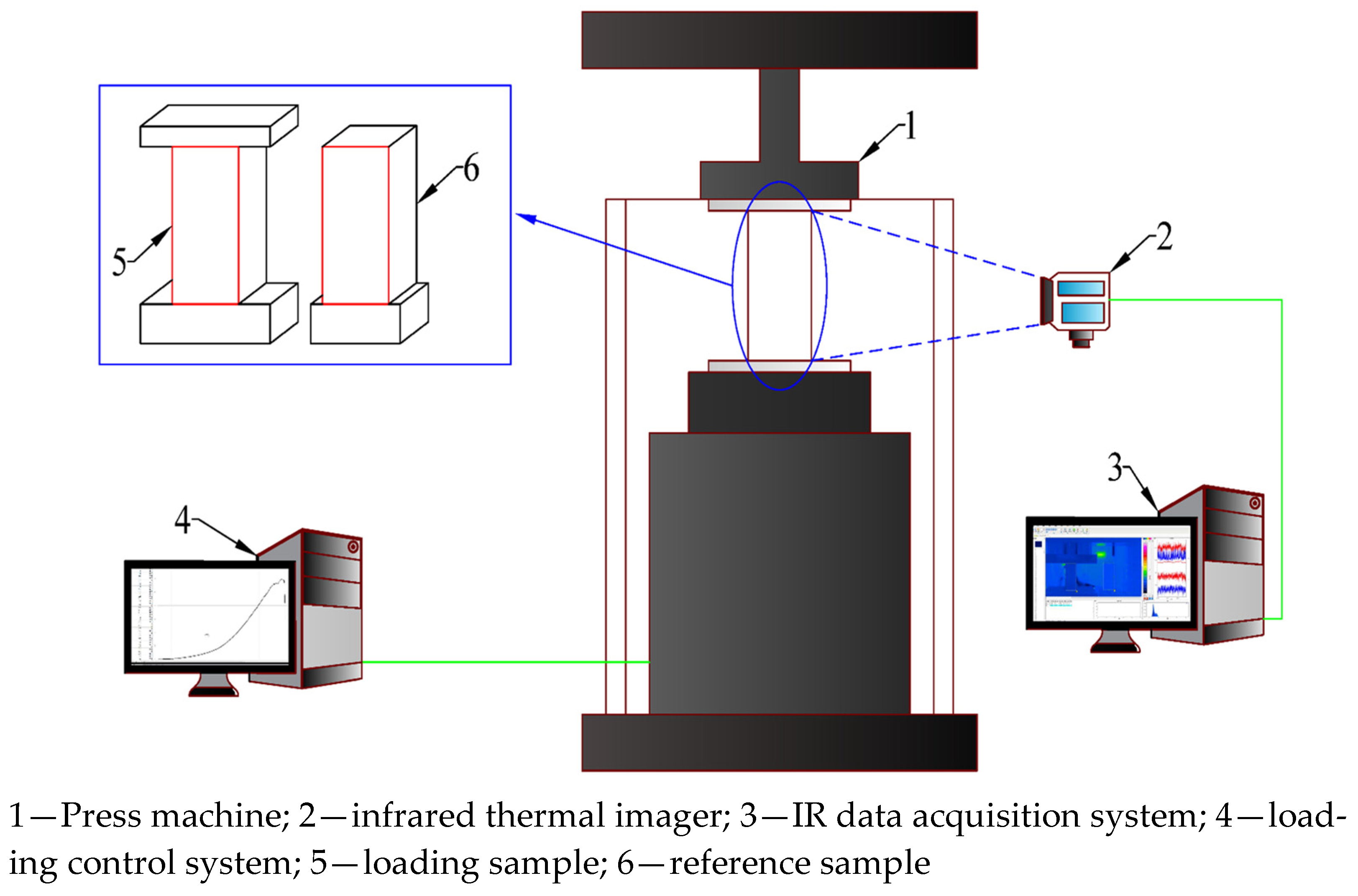
2.2. Experimental Equipment

Infrared (IR) cameras (Model FLIR A615 IR) were placed one meter away from the rock samples, as shown in Figure 1. The IR camera can capture images at a resolution of 640 × 480 pixels and a wavelength of 7.5~14 μm. Prior to being placed in the loading machine, the rock samples’ ends were wrapped in plastic to prevent any end effects or heat conductions. The loading rate of 0.1 mm/min and the fps IR imager capture rate of 25 were kept constant throughout the studies.

2.3. Mechanical Parameters

Elasticity Modulus

The intact rock elastic modulus (E) is the primary mechanical characteristic that influences rock deformation and determines the slope of the stress–strain curve. Three techniques may be used to compute it: average, tangent, and secant modulus [65]. In this research, assuming that stress is a function of strain, the average modulus (E) was employed. Equation (1) can be used to calculate the value of E.

$$\mathrm{E}=\frac{\mathrm{Z}\left({\mathrm{\epsilon }}_2\right)-\mathrm{Z}\left({\mathrm{\epsilon }}_1\right)}{{\mathrm{\epsilon }}_2-{\mathrm{\epsilon }}_1}$$

(1)

where Z(ε₂) is peak stress, Z(ε₁) is stress at the beginning of the elastic deformation stage, ε₂ is the strain at the peak stress point, and ε₁ is the strain at the beginning of the elastic deformation stage.

2.4. Index

2.4.1. Brittleness Index Base on Stress–Strain Curve

The stress–strain curves collected during the loading of rocks give a clear representation of their characteristics, making them very easy to analyze due to their intuitive nature. Therefore, numerous brittleness indices have been developed, all of which are based on the analysis of the structure and behavior of uniaxial and triaxial compressive stress–strain curves. These indices aim to quantify the brittleness characteristics of rock materials and provide valuable insights into their mechanical response under different loading conditions. These curves provide beneficial insights into the behavior of rocks under various loading scenarios and serve as a foundation for understanding the mechanical properties of rocks. Therefore, the stress–strain curves acquired from rock loading play an essential part in the construction of brittleness indices and provide an in-depth knowledge of rock characteristics. These curves may be created by loading rocks with a variety of loads [8]. Indeed, stress–strain curves resulting from loading rocks are the most direct and intuitive representations of rock properties. When considering uniaxial or triaxial compressive stress conditions, various deformation, stress, and energy values extracted or derived from pre- or post-peak stress–strain curves are frequently employed as indicators of rock brittleness. These indicators provide valuable information about how rocks respond to loading and can aid in assessing their propensity for brittle behavior. One of the most famous brittleness indices was calculated by using ultimate strength and its corresponding strain value as given in Equation (2) [21].

$${{\displaystyle B}}_1=\frac{{\mathrm{\sigma }}_p}{{\mathrm{\epsilon }}_p}$$

(2)

where σ_p is peak stress and ε_p is peak strain.

Wang [66] conducted theoretical analysis and made preliminary calculations to establish a fundamental connection between the initial stress of brittle rock and brittleness indices. These indices were based on the ratio between the rock’s compressive strength and its tensile strength. Instead of factoring in the corresponding strain of the initial stress, they simply used the initial stress value from the stress–strain curve to define brittleness (B₂–B₄). However, this approach has led to conflicting outcomes compared to calculations-based elastic modulus and energy consideration. Furthermore, the results obtained are inconsistent and lack a smooth, continuous pattern. These indices are calculated by using Equations (3)–(5).

$${{\displaystyle B}}_2=\frac{{{\displaystyle 8\mathrm{\sigma }}}_p}{{\mathrm{\sigma }}_i}$$

(3)

$${{\displaystyle B}}_3=\frac{{{\displaystyle {\mathrm{\sigma }}_i\mathrm{\sigma }}}_p}{16}$$

(4)

$${{\displaystyle B}}_4=\sqrt{\frac{{{\displaystyle {\mathrm{\sigma }}_i\mathrm{\sigma }}}_p}{16}}$$

(5)

where σ_i is crack initiation and σ_p is peak stress.

2.4.2. Infrared Radiation Variance (IRV)

The IR index means that IRV is frequently employed in the loading process for rock fracture detection. This works out the spread of the IR temperature on the sample’s surface. Changes in surface temperature can be depicted by variance when the sample deforms and damage. The IR image sequence matrix is determined using Equation (6).

$$IR{V}_x=\frac{1}{R}\frac{I}{C}{\sum }_{t=1}^C{\sum }_{s=1}^R[f_k(s,t)-AIR{T}_x{]}^2$$

(6)

where $x$ represents the image (IR) sequence frame number index, $s$ represents row, and $t$ represents the thermograph matrix’s column. AIRT_x in Equation (6) is represented as Equation (7).

$$AIR{T}_x=\frac{1}{R}\frac{I}{C}{\sum }_{t=1}^C{\sum }_{s=1}^R{f}_x(s,t)$$

(7)

where $C$ and $R$ are the maximum columns and rows.

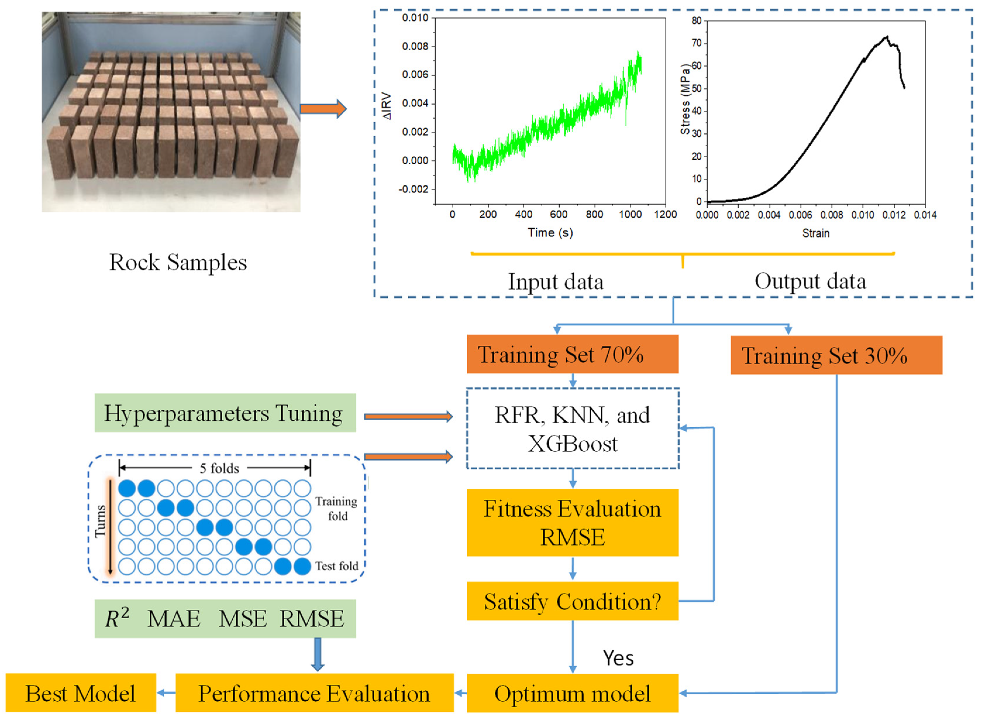
2.5. Artificial Intelligent Techniques

2.5.1. Random Forest Algorithm

The standard Python package known as Scikit-learn (sometimes spelled sk-learn) is used to build the random forest algorithm (RFR), also known as the random forest learning algorithm. In the field of machine learning, RFR is categorized as an ensemble approach that was first presented by [66]. Classification and regression analysis are two of the applications that make use of this tree-based method. RFR generates trees by randomly picking and replacing subsets of variables from the initial dataset. In this way, it successfully incorporates both category and numerical information to handle difficulties relating to prediction. Random forests include a feature called built-in cross-validation that allows for ranking the relevance of the explanatory variables, which indicates the strength of correlation that each component has with the outcome variable [67]. RFR is a method that is often used in the discipline of rock engineering, specifically for predicting ground movement, rock pillar stability, and landslides [13,48,68,69,70].

The request for proposal (RFP) typically incorporates two key components: the decision tree (DT) approach and the bagging technique. The DT approach is versatile and can be utilized to address both classification and regression problems. However, the choice of application depends on the characteristics of the dataset at hand. In order to prepare the feature space for the DT method, it is first subdivided into several smaller parts. Iteratively, the splitting is carried out up to the point when the stop threshold is reached [66].

DT is made up of three different parts: the internal, the external, and the branch. The internal nodes are inextricably tied to decision-making skills to establish which node should be contacted next. The terminals or leaf nodes are another name for the output nodes that can no longer be split. In diverse geotechnical engineering scenarios, the DT technique may be helpful and provide positive results. On the other hand, the RF method is superior in terms of efficiency and precision to using a single tree in various data processing applications. By outfitting control and averaging the DT, the reliability of the model may be enhanced [71]. The regression model known as RF may be written down as [72].

$$\mathit{P}=\frac{\mathbf{1}}{\mathit{s}}{\displaystyle {\sum }_{\mathit{i}=\mathbf{1}}^{\mathit{s}}}{\mathit{F}}_{\mathit{i}}(\mathit{Q})$$

(8)

The input feature factor is denoted by Q, the prediction outcome is denoted by P, and the number of regression trees generated is denoted by S. Figure 2 illustrates the fundamental components that make up RF. In this context, “n” represents the total number of trees constructed in an RF and “Result-1,” “Result-2,” up to “Result-n” represent the outcomes of each individual decision tree (DT).

2.5.2. KNN

The nearest neighbor machine learning methods make predictions based on the closest data points in the training set. K-nearest neighbor (KNN) algorithm is a specific variant that selects the k-closest neighbors to an input point and uses their labels or values to make predictions. This algorithm is particularly efficient when dealing with large datasets and low-dimensional feature spaces. However, it can become computationally expensive in high-dimensional spaces due to the curse of dimensionality. KNN can be adapted to different machine learning problems by adjusting the output function or distance metric used to measure the similarity between data points. For instance, multi-label classification can be accomplished by changing the KNN output function to assign labels based on the most common labels among the K neighbors. Regression can be achieved by taking the average or weighted average of the K nearest values. Semi-supervised learning can be implemented using KNN to propagate labels from labeled to unlabeled data points based on their proximity in the feature space [73].

The KNN approach is simple, effective, and easy to use. This technique is similar to ANN and RFR for classification and regression [74]. The major aim of this technique is to find a group of “k” samples close to the unidentified samples in the dataset (using distance functions). Moreover, in KNN, unidentified samples are categorized by averaging their responses and interpreting the outcomes using the “k” samples [75]. The efficiency of KNN is heavily reliant on the value of k. When addressing regression problems, Equations (9)–(11) employ three distance functions to calculate the separation between neighboring points.

$$\mathit{F}\left(\mathit{a}\right)=\sqrt{{\displaystyle {\sum }_{\mathit{i}=\mathbf{0}}^{\mathit{f}}}{\left({\mathit{k}}_{\mathit{i}}-{\mathit{l}}_{\mathit{i}}\right)}^{\mathbf{2}}}$$

(9)

$$\mathit{F}\left(\mathit{m}\mathit{b}\right)=\sqrt{{\displaystyle {\sum }_{\mathit{i}=\mathbf{0}}^{\mathit{f}}}\left|{\mathit{k}}_{\mathit{i}}-{\mathit{l}}_{\mathit{i}}\right|}$$

(10)

$$\mathit{F}\left(\mathit{m}\mathit{c}\right)={\left(\sqrt{{\displaystyle {\sum }_{\mathit{i}=\mathbf{0}}^{\mathit{f}}}{\left(\left|{\mathit{k}}_{\mathit{i}}-{\mathit{l}}_{\mathit{i}}\right|\right)}^{\mathit{t}}}\right)}^{\frac{\mathbf{1}}{\mathit{t}}}$$

(11)

In the given context, the notation can be interpreted as follows:

• $F\left(a\right)$ represents the Euclidean function, which calculates the distance between two points using the Euclidean distance metric.
• $F\left(mb\right)$ represents the Manhattan function, which calculates the distance between two points using the Manhattan distance metric.
• $F\left(mc\right)$ represents the Minkowski function, which calculates the distance between two points using the Minkowski distance metric. The specific value of t indicates the order or power used in the Minkowski distance calculation.
• $k_i$ and l_i represent the respective coordinates or values of the ith dimension for points k and l.
• $t$ represents the order or power used in the Minkowski distance calculation.

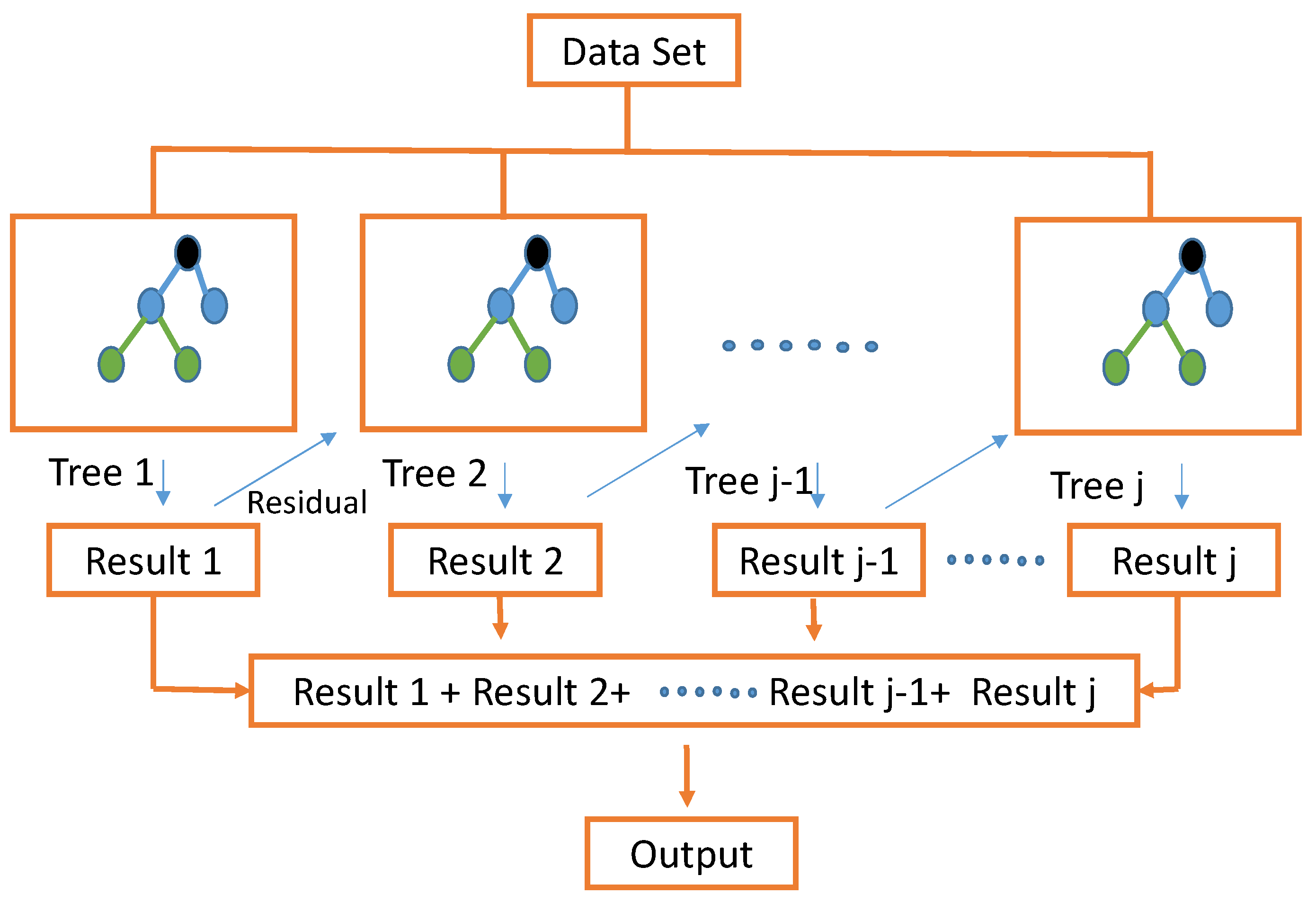
2.5.3. Extreme Gradient Boosting

Extreme gradient boosting, or XGBoost, is an effective, adaptable, scalable, gradient-boosted decision tree (GBDT) deep learning package. It was developed by Tianqi Chen and Guestrin [76]. The XGBoost model’s structural details are shown in Figure 3.

It is better for the classification of large datasets according to their complexity or priority required to attain a solution until the last step for obtaining the result. This method provides a sequential manner for placing the tree in an algorithmic way, which gives the advantage of reducing the overfitting of the data. This algorithm arranges the datasets in such a way that each problem is ranked accordingly, and its associated tasks are shown as a tree in parallel. A possible use of the XGBoost algorithm is to incorporate it into machine learning because of its capability to take care of large datasets efficiently and help recover the missing data as well. The main problems are classified accordingly. It is based on the fact that when the best possible next model is combined with the previous method, the prediction of the model to be analyzed at the end of the algorithm should have minimum error. The machine learning concept employed in this algorithm is to set the target outcomes for the next model in order to minimize the error. This method is carried out from top to bottom until the combined result from each tree gives the correct outcome efficiently [77].

3. Results and Discussion

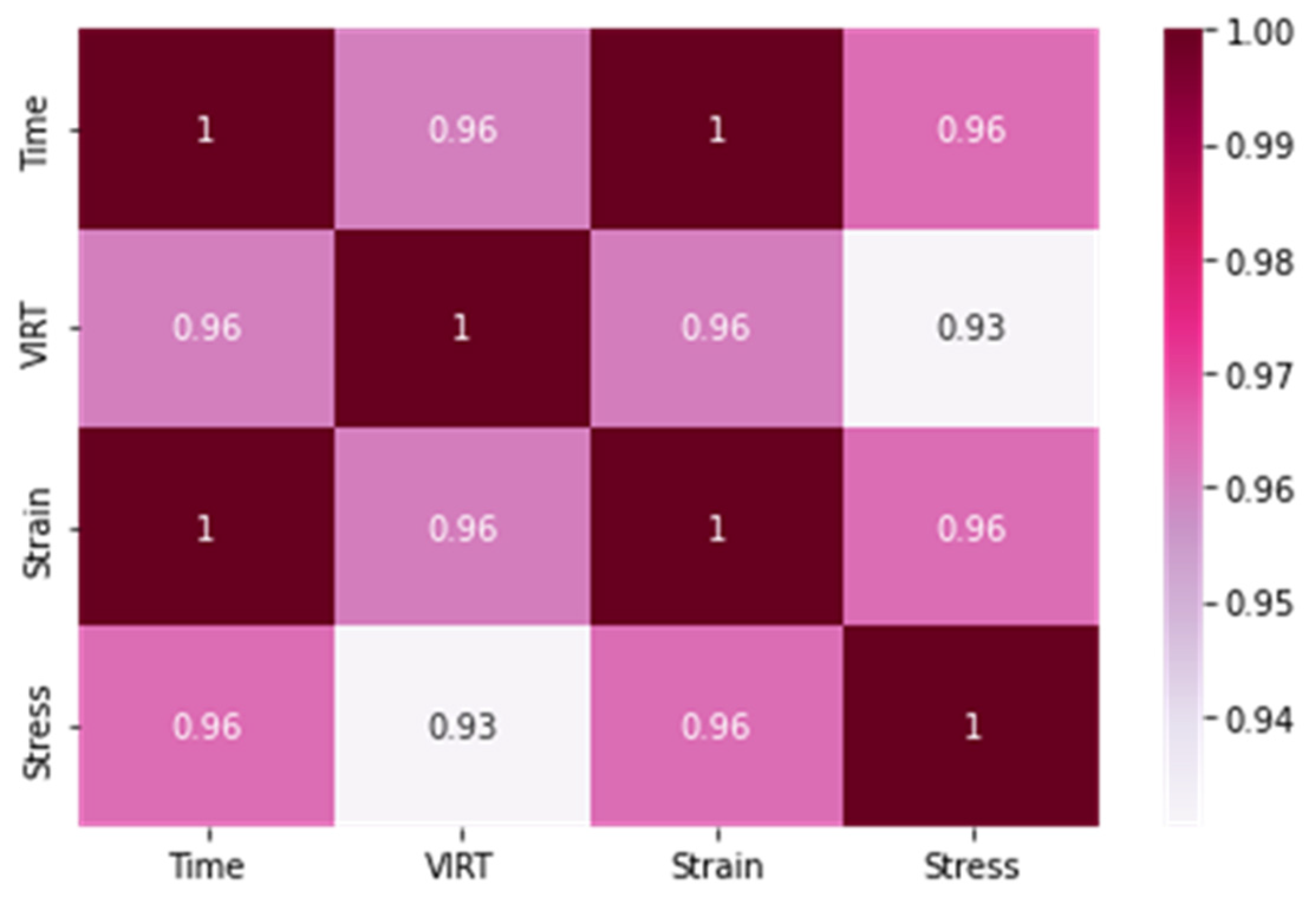
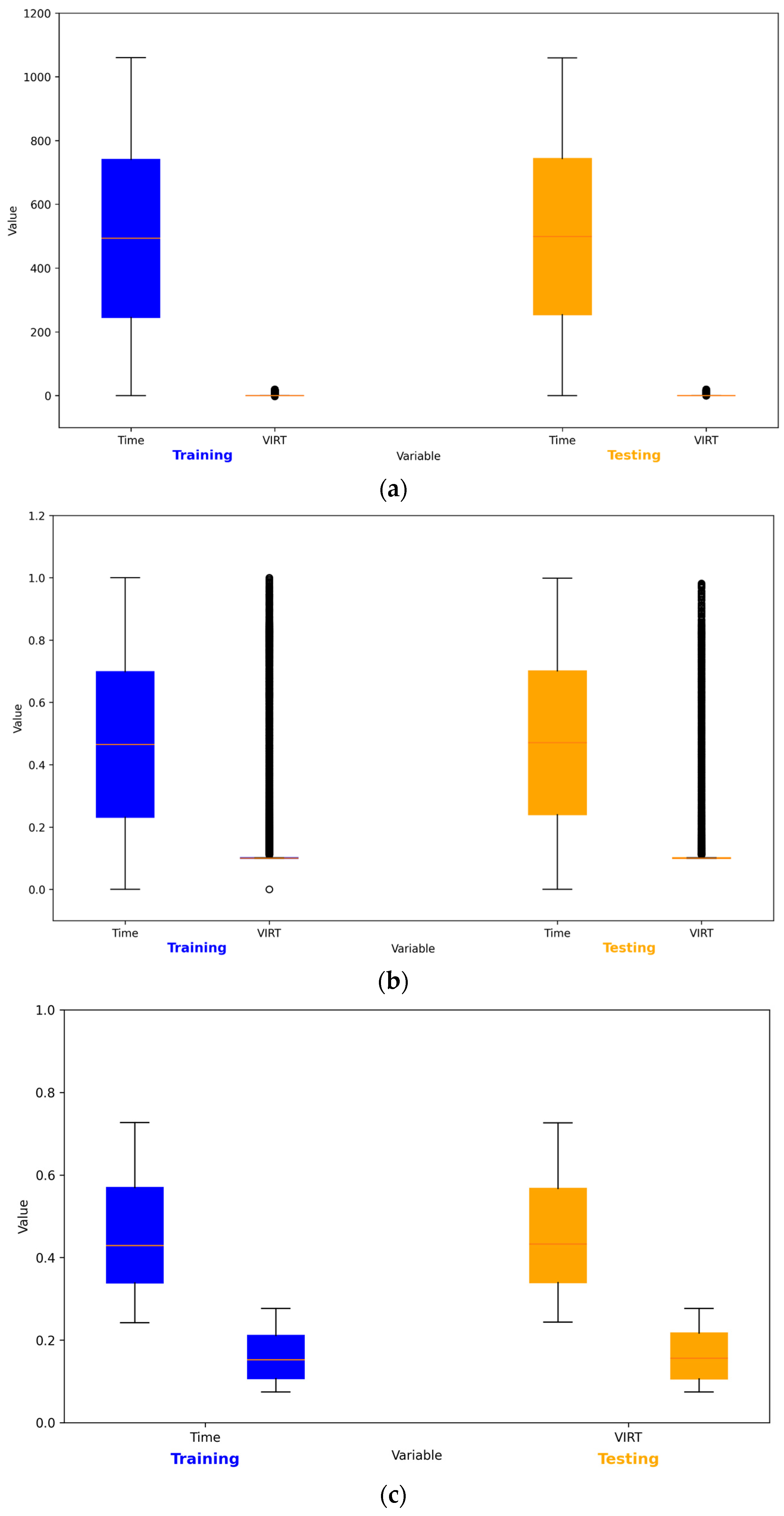
3.1. Data Statistical Analysis

In the current study, the parameters for the machine learning techniques include variables consisting of time, IR, stress, and strain. The inputs, time, and variance of IR are taken into consideration for the forecasting of stress and strain. The results of the statistical analysis of the data for various water contents are represented in

Table 1. Statistical analysis of variables.

Parameters	Mean	Standard Deviation	Minimum	Median	Maximum
Time	473.200	273.130	0.200	473.200	946.200
IR	0.010	0.008	0.000	0.008	0.028
Strain	0.010	0.000	0.000	0.010	0.010
Stress	20.430	18.163	0.005	15.518	55.053

.

Figure 4 shows the heat diagram, which indicates that the independent variable strongly correlates with the dependent variable. It also reveals that the independent variables also have a very good correlation with each other, revealing that both the independent variables are good at predicting the stress–strain curve.

In this study, the data were split into 70% for training and 30% for testing. To analyze the distribution of each indicator, the data were scaled and normalized to a range of (0,1). This normalization process allows for a fair comparison of the data across different indicators. The resulting boxplot in Figure 5 displays the distribution of each indicator. By observing the boxplots, it becomes evident that the data distributions vary across different indicators, confirming their independence. This highlights the importance of considering all input indicators collectively to enhance the accuracy of the analysis. Furthermore, it is worth noting that the distributions of the training and test sets for each input indicator exhibit similarities. This similarity indirectly validates the random partitioning of the data, further ensuring the reliability of the analysis. Figure 5a elucidates the data without normalization, which shows that the data are dispersed in VIRT. Figure 5b replicates the normalized data, which also reveals that the data consist of an outlier. Figure 5c shows the normalized data without the outlier. The outlier in Figure 5c is removed and now the data almost show a normal distribution.

3.2. Effect of Water on Stress–Strain

The presence of water in rock masses substantially influences their susceptibility to damage, resulting in a decrease in their mechanical properties [78]. This occurs due to various factors, such as the weakening of interparticle bonds, chemical reactions, increased pore pressure, and the promotion of microcrack growth. Consequently, the mechanical qualities of the rock are negatively impacted, rendering it more vulnerable to deformation and failure. As a direct result of this, the saturated rock that is subjected to stress evidences a reduction in the amount of dissipation strain energy that is available for fracture processes of water, whereas the crack closure and the unstable crack propagation stages increase. Khan et al. [79] provide a description of the mechanical characteristics of stress–strain curves in various water contents. They show that the peak stress, elastic modulus, crack damage stress, and crack initiation stress are inversely proportional to the content of water due to the lubricating effect of water, which accelerates the weakening effect of rock and speeds up the pace at which tension is released.

Table 2. Mechanical properties of different water-bearing sandstone specimens.

Samples No.	Water Content (%)	E (GPa)	σp (MPa)	ϵp 10−2	σi (MPa)	σd (MPa)
K-1	0.0000	10.1310	73.1210	1.2510	41.8100	63.3810
K-2	0.0000	9.8710	74.5810	0.9940	37.2300	62.2900
K-2	0.0000	9.4620	69.5520	0.8820	37.7410	57.1330
L-1	0.9710	8.7510	57.7910	1.0330	26.8200	44.1020
L-2	1.1350	8.9800	60.7720	1.1300	31.7500	42.4010
L-3	0.9910	9.3700	64.5310	1.2600	31.6000	49.6900
M-1	2.0750	7.2500	51.9230	1.1740	24.3320	38.4420
M-2	2.1360	7.9910	49.8420	1.2520	22.5500	34.9020
M-3	1.9540	7.8820	48.8930	1.1930	21.5600	33.7000
N-1	3.1090	5.8810	41.9710	1.1810	17.7910	28.1510
N-2	3.0040	5.4320	38.0320	1.2420	15.8500	28.1020
N-3	3.1130	4.8830	36.5710	1.2310	16.1800	26.3900

Note: E: elastic modulus, σ_p: peak stress; ϵ_p: peak strain, σ_i: crack initiation stress, σ_d: crack damage.

presents the important mechanical properties of sandstone for a range of different water concentrations. The result is consistent with [79].

Initiation of Crack and Crack Damage Stress

To determine the stresses related to rock crack closure, crack initiation, and dilatancy, the strain–stress and stiffness–stress curves were analyzed at different water concentrations. By examining these curves, the stresses associated with each phenomenon can be calculated and assessed. Samples with different water contents were subjected to uniaxial loading, resulting in the generation of strain–stress and stiffness–stress curves. Figure 6 and Figure 7 illustrate these curves, providing a visual representation of the response of the samples under varying water content conditions [79]. These figures show strain–stress and stiffness–stress curves, respectively. Point O is the origin of the initial loading point in the loading process. These curves will grow to the point of intersection, known as the crack closure stage (point A). The spot on the stiffness–stress curve where it reaches its maximum curvature is referred to as the crack initiation point (B). This point is determined as a function of loading time. The stage from A to B is known as the elastic deformation stage.

Point C on the stress–stiffness curve represents the maximum point where the curve rises to its peak. At this point, there is a sharp decline in the curve, indicating the dilatancy point. The stress level at this instance is referred to as the dilatancy stress.

The section from B to C represents the progressive growth stage of the crack. As the loading continues, the curve reaches point D, which represents the maximum allowable stress that the sample can withstand before failure.

At the CD stage, while the crack is still growing unstably, the sample may be heard clearly. As the sound waves travel through the material, the tiny cracks grow, spread, and eventually collide. Macrocracks appear; however, the loaded samples are still intact.

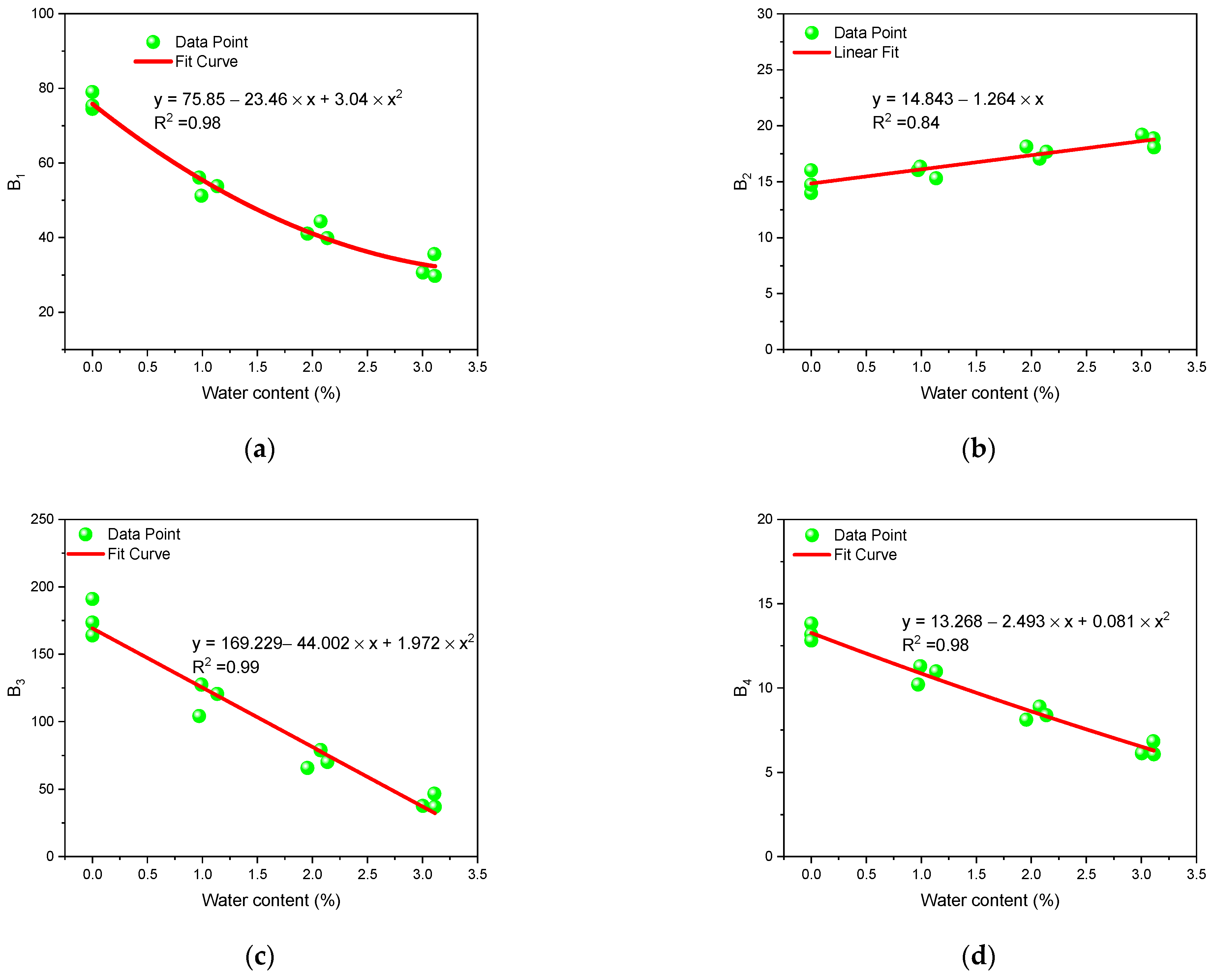
3.3. Effect of Water Content on Rock Behaviors

Water is a significant factor in geological disasters that affect rock engineering because it tends to collect in the small cracks and spaces within rocks. When water interacts with rocks, it can lead to a range of physical, chemical, and mechanical changes that alter the original internal structure of the rock [80]. As a result of water exposure, rocks may exhibit varying degrees of reduced brittleness and strength compared to their dry state. The extent of these changes can depend on factors that vary with rock type and the duration and amount of water exposure [81]. Figure 8a shows the water content and brittleness (B₁) relationship. It reveals that there is a quadratic correlation between B₁ and water content. This relationship is inversely proportional, having a coefficient of determination of R² = 0.98. Figure 8b reveals a linear correlation between B₂ and water content. The relation is positive, which means that, with an increase in water content, the B₂ value increases. This means that the intensity of brittleness decreases when the B₂ increases above 10. Figure 8c shows a quadratic correlation between B₃ and water content. This relationship is inversely proportional, having a coefficient of determination of R² = 0.99. Similarly, B₄ shows a quadratic correlation between B₃ and water content, having a coefficient of determination of R² = 0.98 as shown in Figure 8d. Mathematically, all relationships of B₁, B₂, B₃, and B₄ with water can be calculated using Equations (12)–(15), respectively.

$${\mathrm{B}}_1=75.85 - 23.46 \mathrm{x}+3.04{ \mathrm{x}}^2\hspace{1em}{R}^2=0.98$$

(12)

$${\mathrm{B}}_2=14.843 - 1.264 \mathrm{x}\hspace{1em}{R}^2=0.84$$

(13)

$${\mathrm{B}}_3=169.229- 44.002 \mathrm{x}+1.972{ \mathrm{x}}^2 \hspace{1em}{R}^2=0.99$$

(14)

$${\mathrm{B}}_4=13.268 - 2.493 \mathrm{x}+0.081{ \mathrm{x}}^2\hspace{1em}{R}^2=0.98$$

(15)

where x is water content.

Figure 9a shows the elastic modulus and brittleness (B_1, B₂, B₃, and B₄) relationship. This reveals that there is a positive exponential linear correlation between B₁ and elastic modulus, having a coefficient of determination of R² = 0.86. Figure 9b reveals a negative exponential linear correlation between B₂ and elastic modulus, having a coefficient of determination of R² = 0.86. The relation is inverse, which means that with an increase in water content, the B₂ value decreases. This means that the intensity of brittleness decreases when B₂ increases above 10. Figure 9c shows a positive exponential linear correlation between B₃ and elastic modulus, having a coefficient of determination of R² = 0.97. Similarly, B₄ shows a positive exponential linear correlation between B₃ and elastic modulus, having a coefficient of determination of R² = 0.97 as shown in Figure 9d. Mathematically, all relationships of B₁, B₂, B₃, and B₄ with elastic modulus under different water contents can be calculated using Equations (16)–(19), respectively.

$${\mathrm{B}}_1{=\mathrm{e}}^{\frac{E}{2.252}} -0.721\mathrm{E}+28.676\hspace{1em}{R}^2=0.86$$

(16)

$${\mathrm{B}}_2=12.882+5.889{\mathrm{e}}^{\frac{-2{(E-5.845)}^2}{30.969}}\hspace{1em}{R}^2=0.86$$

(17)

$${\mathrm{B}}_3=0.881{\mathrm{e}}^{\frac{E}{1.912}}-1.326\mathrm{E}+32.916 R^2=0.97$$

(18)

$${\mathrm{B}}_4=0.103{\mathrm{e}}^{\frac{E}{2.336}}-0.172\mathrm{E}+4.389 R^2=0.97$$

(19)

Figure 10a shows the crack initiation stress and brittleness (B_1, B₂, B₃, and B₄) relationship. This reveals that there is a positive exponential linear correlation between B₁ and crack initiation stress, having a coefficient of determination of R² = 0.92. Figure 10b reveals a negative exponential linear correlation between B₂ and crack initiation stress, having a coefficient of determination of R² = 0.90. The relation is inverse to brittleness intensity, which means that, with an increase in water content, the B₂ value increases. This means that the intensity of brittleness decreases when the B₂ increases above 10. Figure 10c shows a positive exponential linear correlation between B₃ and crack initiation stress, having a coefficient of determination of R² = 0.99. Similarly, B₄ shows a positive exponential linear correlation between B₃ and elastic modulus, having a coefficient of determination of R² = 0.99 as shown in Figure 10d. Mathematically, all relationships of B₁, B₂, B₃, and B₄ with crack initiation stress under different water contents can be calculated using Equations (20)–(23), respectively.

$$\begin{array}{l}{\mathrm{B}}_1=4850.054 -4850.447\times {\mathrm{e}}^{-3.927{\mathrm{\sigma }}_i}{ \mathrm{R}}^2=0.92 \\ \end{array}$$

(20)

$$\begin{array}{l}{\mathrm{B}}_2=4.235{\mathrm{e}}^{-\frac{{\mathrm{\sigma }}_i}{18.298}}-0.123{\mathrm{\sigma }}_i+19.060{ \mathrm{R}}^2=0.90\\ \end{array}$$

(21)

$$\begin{array}{l}{\mathrm{B}}_3=4768.010{\mathrm{e}}^{\frac{{\mathrm{\sigma }}_i}{120.674}}-1.979{\mathrm{\sigma }}_i-808.706{ \mathrm{R}}^2=0.99\\ \end{array}$$

(22)

$$\begin{array}{l}{\mathrm{B}}_4=-0.581{\mathrm{e}}^{\frac{{\mathrm{\sigma }}_i}{20.465}}+0.424{\mathrm{\sigma }}_i+0.610{ \mathrm{R}}^2=0.99\end{array}$$

(23)

Figure 11a shows the crack damage stress and brittleness (B_1, B₂, B₃, and B₄) relationship. This reveals that there is a positive exponential linear correlation between B₁ and crack initiation stress, having a coefficient of determination of R² = 0.94. Figure 11b reveals a negative exponential linear correlation between B₂ and crack initiation stress, having a coefficient of determination of R² = 0.82. The relation is inverse, which means that, with an increase in water content, the B₂ value increases. This means that the intensity of brittleness decreases when B₂ increases above 15. Figure 11c shows a positive exponential linear correlation between B₃ and crack initiation stress, having a coefficient of determination of R² = 0.98. Similarly, B₄ shows a positive exponential linear correlation between B₃ and elastic modulus, having a coefficient of determination of R² = 0.98 as shown in Figure 11d. Mathematically, all relationships of B₁, B₂, B₃, and B₄ with crack initiation stress under different water contents can be calculated using Equations (24)–(27), respectively.

$$B_1=0.230e^{\frac{{\mathrm{\sigma }}_c}{1.845}}+1.274{\mathrm{\sigma }}_c-3.382 R^2=0.94$$

(24)

$$B_2=645.163e^{-\frac{{\mathrm{\sigma }}_c}{1.845}}+1.503{\mathrm{\sigma }}_c-619.251 R^2=0.82$$

(25)

$$B_3=2.365e^{\frac{{\mathrm{\sigma }}_c}{5.637}}+4.055{\mathrm{\sigma }}_c-72.840 R^2=0.98$$

(26)

$$B_4=0.852e^{\frac{{\mathrm{\sigma }}_c}{1.166}}+0.203{\mathrm{\sigma }}_c-0.252 R^2=0.98$$

(27)

The above relationships between brittleness and indices and crack initiation, crack damage, and elastic modulus show a high coefficient of determination, with an average above 0.82. The presence of water directly affects the brittleness (reduces the brittleness by 41% (average)) of rocks, as well as their mechanical properties, such as strength, elastic modulus, crack initiation, and damage. Inverse relationships exist between the water content and these mechanical properties. It can be concluded that rocks with a higher water content exhibit lower brittleness compared to dry conditions, resulting in a decreased rock strength and elastic modulus.

Furthermore, the stages of rock loading play a significant role in rock brittleness. Higher rock brittleness corresponds to less crack closure and a stable crack propagation stage, while elastic and unstable crack propagation stages become more prominent. Conversely, lower rock brittleness is associated with increased crack closure and stable crack propagation. These relationships are illustrated in Figure 5.

3.4. Proposed Brittleness Index under Stress–Strain Condition

The content of water has a considerable impact on the proportional strain and stress at several stress–strain curve phases, including elastic deformation, crack closure, and stable and unstable crack prorogations. This water content leads to a proportional increase in strain and decrease in stress at different stages. Different authors used different brittleness indices for different materials and conditions, as summarized by Meng, Wong, and Zhou [19]. In this study, the authors proposed an index considering crack initial stress, crack damage stress, and peak stress. In water content conditions, crack initiation and damage and peak stress are reduced with water content. Moreover, this is not proportionally decreased with water content. Therefore, a brittleness index that can consider these three kinds of stresses under different conditions of water content and reflect the brittleness of rock under water content conditions is important for avoiding rock burst in deep underground mining. The brittleness of rock under water conditions is reduced, and its impact is less pronounced compared to dry conditions. Consequently, in highly brittle rock formations, increased water content diminishes the rock’s brittleness and concurrently mitigates the occurrence of rockburst phenomena. Previous studies have not adequately accounted for the influence of water content on the effectiveness of brittleness. The proposed brittleness index takes into account all three stress (crack initial stress, crack damage stress, and peak stress) affected by varying water contents. It can be calculated by using Equation (28).

$$B_{IDP}=\frac{1}{1000{\mathrm{\sigma }}_i}\times E{\mathrm{\sigma }}_p{\mathrm{\sigma }}_d$$

(28)

where B_IDP is the brittleness index, σ_d is crack damage stress, σ_i represents crack initiation stress, and peak stress is represented by σ_p.

Figure 12 shows the proposed brittleness (B_IDP) and previous brittleness (B₁, B₂, B₃, and B₄) relationship, which reveals a strong linear correlation (R² = 0.87) with B₁, B₃, and B₄ and weak negative linear correlation (R² = 0.61) with B₂. The coefficient of determination of the proposed B_IDP and previous brittleness indices B₁, B₃, and B₄ is greater than 0.80, so this can be used in engineering [82]. The details of the intensity of brittleness for the proposed index are given in

Table 3. Brittleness intensity range for proposed index.

Indices	Intensity of Brittleness
	Extreme	High	Intermediate High	Middle	Low
BIDP	>100	90–100	80–90	70–80	<70

.

Table 4. Intensity comparison of proposed and existing brittleness indices.

Samples	Water Content	Previous Brittleness Indices						Proposed Brittleness Indices
No.		B1	Grade	B2	B3	B4	Grade	BIDP	Grade
K-1	0.0000	58.4960	Extremely	13.9911	191.0743	13.8230	Moderate	110.8463	Extremely
K-2	0.0000	75.3330	Extremely	16.0260	173.5407	13.1735	Moderate	124.7824	Extremely
K-2	0.0000	79.0340	Extremely	14.7430	164.0601	12.8086	Moderate	105.2891	Extremely
L-1	0.9710	56.1070	Extremely	16.0419	104.0960	10.2027	Moderate	88.4351	Moderate
L-2	1.1350	53.7790	Extremely	15.3126	120.5944	10.9815	Moderate	81.1589	Moderate
L-3	0.9910	51.2140	Extremely	16.3370	127.4487	11.2893	Moderate	99.4308	High
M-1	2.0750	44.3760	Extremely	17.0715	78.9619	8.8861	Brittle	82.0329	Moderate
M-2	2.1360	39.8720	High	17.6823	70.2461	8.3813	Brittle	77.1435	Low
M-3	1.9540	41.0840	Extremely	18.1421	65.8833	8.1169	Brittle	76.4237	Low
N-1	3.1090	35.5680	Extremely	18.8729	46.6691	6.8315	Brittle	66.4114	Low
N-2	3.0040	30.6690	Extrmely	19.1960	37.6755	6.1380	Brittle	67.4306	Low
N-3	3.1130	29.7310	Brittle	18.0821	36.9824	6.0813	Brittle	59.6483	Low

reveals the intensity of different brittleness indices with the proposed index. It shows that the existing index B₁ gives a brittleness intensity grade that is extremely high in water content, which does not reflect the true picture of the brittleness of rock in the current study. Similarly, B₂, B₃, and B₄ do not reflect the actual condition of the rock brittleness under loading in different water contents, whereas these indices represent some brittleness better than B₁. The difference in the actual and calculated brittleness is due to a leak of some parameters that are strongly affected by water content that are missing in B₁, B₂, B₃, and B₄ indices. In the proposed brittleness B_IDP, the overall mechanical parameter is considered, which truly reflects the actual brittleness condition.

3.5. Brittleness Index Using IRV under Different Water Conditions

Figure 13 reveals the relationship between brittleness and ∆IRV. It shows that the brittleness and ∆IRV have a negative quadratic relationship with R² = 0.90 in different water contents. The fitting function for brittleness and ∆IRV is as follows:

$$\Delta IRV=92.58 -1.27 \mathrm{B}$$

(29)

where $\mathrm{B}$ is brittleness.

The generalized equation between brittleness and IRV is

$$\Delta IRV=\mathrm{c} - \mathrm{aB}$$

(30)

where c and a are constant

$$\mathrm{B}=\frac{-\Delta IRV}{a}+\frac{c}{a}$$

(31)

where 1/a represents the brittleness infrared radiation coefficient (BIRC) and $\frac{c}{a}$ is the brittleness constant. The rock brittleness is inversely proportional to the BIRC and directly proportional to the brittleness constant.

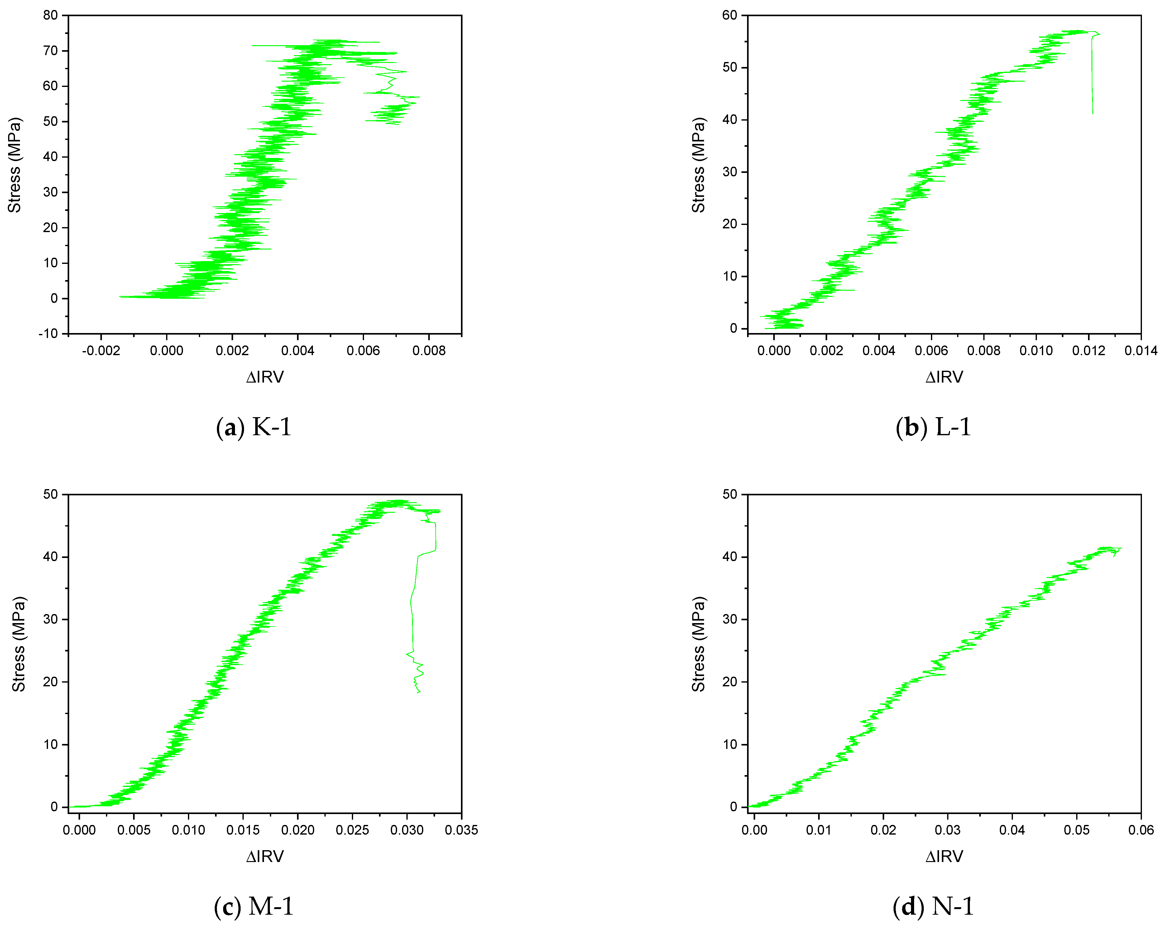
3.6. IRV Characteristic under Stress–Strain Curve Stages

Ma et al. [62] explain the behavior of IRV with stress, as shown in Figure 14. It was found that the IRV characteristic changed depending on the amount of water present at various fracture stages. At fracture closure and during deformation, stable, and unstable crack propagations, the rate of IRV is determined. In dry conditions, their respective values are 0.0018, 0.0034, 0.0035, and 0.0048, with the latter being the lowest of the four. Similarly, these values are 0.01265, 0.01433, 0.02223, and 0.02846 under water content conditions. Additionally, Figure 14 illustrates a clear linear association between stress and IRV. This relationship appears to be more pronounced in water-saturated conditions compared to dry conditions. The presence of water enhances the IRV due to an increased water content. The authors also inferred that an increase in water content leads to a reduction in rock brittleness. This implies a negative linear correlation between IRV and brittleness, where higher rock brittleness corresponds to lower IRV, and vice versa.

According to Khan, Ma, Cao, Hussain, Liu, Xu, Yuan, and Gu [79], stress decreases as water content rises. They explained that whereas the matching IRV has a positive quadratic association with water, the stress at fracture initiation and damage exhibits a negative linear relationship (decreasing). This behavior is brought about via water lubrication, which also causes an increase in fracture damage stress while reducing the rate of crack initiation stress.

3.7. Prediction Models

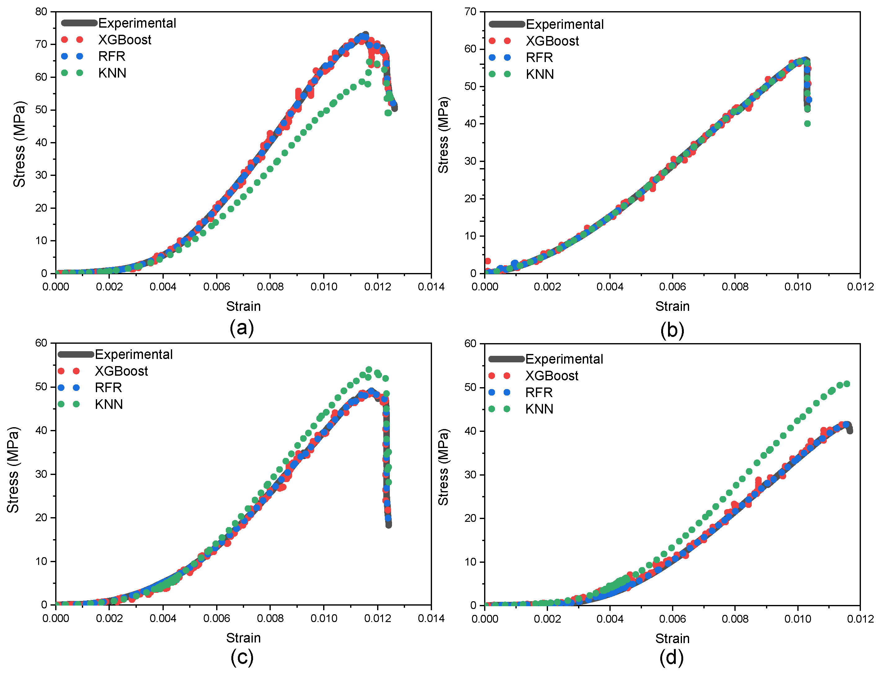
3.7.1. Regression Models

In this study, machine learning algorithms such as KNN, RFR, and XGBoost were employed using the Python Scikit-Learn package. The data were preprocessed by normalizing it to a standard scale before being divided into training and testing sets in a 70–30 split, as shown in Figure 15. During the testing phase, the hyperparameters of each model were adjusted to identify the optimal settings. For RFR and XGBoost, the hyperparameters “n_estimators” (representing the number of decision trees in the model) and “max_depth” (representing the maximum depth of each decision tree) were fine-tuned. In the case of KNN, the “number of neighbors” hyperparameter was adjusted to determine the optimal number of neighbors for the averaging process during forecasting. To find the optimal hyperparameters, a grid search method was utilized, aiming to achieve the highest accuracy while minimizing computational cost [83].

In the grid search method, prospective values for each hyperparameter are exhaustively investigated throughout a broad range, and then the optimal combination of those values is chosen as the method for achieving the desired results. When dealing with large datasets, the computational cost of exploring a wide range of hyperparameter settings can be substantial. However, the primary focus is to enhance the reliability of the results. To identify a feasible range of hyperparameter values, each parameter varies at different levels while keeping the other parameters constant. The optimal values for the hyperparameters of each model are presented in

Table 5. Optimized hyperparameters of all techniques.

Output	Model	Parameters
Stress, Strain	RF	n_estimator = 30, max_depth = 13, random state = 42
	KNN	n_neighbors = 3, metric = Minkowski
	XG Boost	n_estimator = 100, reg_ lambda = 1, max_depth = 3, random state = 10

, which was compiled using grid search. In Figure 16, a comparison is provided between the actual stress–strain data and the predicted stress–strain derived from the model trained with the optimal parameters. This allows for an evaluation of the model’s performance in capturing the observed behavior of the stress–strain relationship.

3.7.2. Performance of Models

The performance of each model was assessed using four different performance indicators: coefficient of determination (R²), root mean square error (RMSE), mean square error (MSE), and mean absolute error (MAE). The optimum word for the model is used when the R² and RMSE values are maximum and minimum, respectively. The details of each model during the training and testing properties phase are described in

Table 6. Model efficiency during training and testing.

S.no	Models	Accuracy (Training)				Accuracy (Testing)
		R2	MAE	MSE	RMSE	R2	MAE	MSE	RMSE
1	XGBoost Regressor	0.998	0.193	0.146	0.382	0.999	0.193	0.147	0.383
2	RF	0.999	0.142	0.078	0.279	0.999	0.164	0.069	0.262
3	KNN	0.853	6.195	60.961	7.807	0.853	6.201	61.017	7.811

. Based on the optimum value of R² and RMSE, the models were reflected through a radar plot as shown in Figure 17, whereas the proposed brittleness index’s actual and predicted values are shown in Figure 18. It can be seen from Figure 18 that the RF and XGBoost predicted values coincide with the actual value, while KNN is near to the actual values but does not coincide with actual values. Between RF and XGBoost, RF is more efficient in the prediction of the brittleness index compared to XGBoost. The models were ranked based on performance indicators as RF > XGBoost > KNN.

RF and XGBoost exhibited notably higher accuracy compared to KNN due to several factors. Firstly, RF and XGBoost are ensemble methods that leverage multiple decision trees. They handle complex relationships within the data more effectively by constructing numerous trees and combining their predictions, resulting in superior predictive power. This ensemble nature allows them to capture intricate patterns and nuances present in the dataset, contributing to their higher accuracy. Additionally, RF and XGBoost are less sensitive to noise and outliers compared to KNN, which can be influenced by irrelevant or redundant features. Moreover, both RF and XGBoost have mechanisms to reduce overfitting by using methods like bagging and boosting, respectively, while KNN can be prone to overfitting due to its reliance on nearby data points. KNN, on the other hand, relies on the proximity of data points for predictions, making it more susceptible to noisy or irrelevant features. It performs well with smaller datasets but struggles when faced with larger datasets or those containing less relevant information. Furthermore, KNN’s prediction accuracy heavily depends on the chosen value of ‘k’ (the number of nearest neighbors), which might not always be optimal for the dataset, leading to reduced accuracy in certain scenarios. The performance indicators were calculated using Equations (32)–(35).

$${\mathrm{R}}^2=\frac{{\displaystyle {\sum }_{\mathrm{i}=1}^{\mathrm{n}}{{(\mathrm{k}}_{\mathrm{i}})}^2-{\displaystyle {\sum }_{\mathrm{i}=1}^{\mathrm{n}}{{(\mathrm{k}}_{\mathrm{i}}{-\mathrm{l}}_{\mathrm{i}}^{\prime })}^2}}}{{\displaystyle {\sum }_{\mathrm{i}=1}^{\mathrm{n}}{{(\mathrm{k}}_{\mathrm{i}})}^2}}$$

(32)

$$\mathrm{RMSE}=\sqrt{\frac{{\displaystyle {\sum }_{\mathrm{i}=1}^{\mathrm{n}}{(\mathrm{k}}_{\mathrm{i}}{-\mathrm{l}}_{\mathrm{i}}^{\prime })}}{\mathrm{n}}}$$

(33)

$$\mathrm{MSE}=\frac{{\displaystyle {\sum }_{\mathrm{i}=1}^{\mathrm{n}}{(\mathrm{k}}_{\mathrm{i}}{-\mathrm{l}}_{\mathrm{i}}^{\prime })}}{\mathrm{n}}$$

(34)

$$\mathrm{MAE}=\frac{{\displaystyle {\sum }_{\mathrm{i}=1}^{\mathrm{n}}\left|{(\mathrm{k}}_{\mathrm{i}}{-\mathrm{l}}_{\mathrm{i}}^{\prime })\right|}}{\mathrm{n}}$$

(35)

The value of the actual data point is represented by k, the value of the predicted data point is represented by l′, and n shows the total number of points.

The RF model emerges as a robust predictor of the brittleness index, showcasing superior efficiency by closely aligning with actual values and securing the highest rank based on performance indicators. Its capacity to handle large datasets while minimizing overfitting underscores its strength, although computational demands and interpretability challenges persist. KNN demonstrates simplicity and adaptability for smaller datasets, approximating actual values moderately well; however, sensitivity to the k-value and susceptibility to irrelevant features pose limitations. Gradient boosting (XGboost) secures a noteworthy position in performance but demands meticulous tuning, risks overfitting, and may not be optimal for real-time applications or extensive datasets. These models exhibit varying strengths and limitations in predicting the brittleness index, warranting consideration of their trade-offs in different analytical contexts.

3.7.3. Models Strength and Limitation

Random forest (RF) showcases robustness in handling vast datasets and features, minimizing overfitting through ensemble learning from multiple decision trees. Its ability to estimate feature importance aids in effective variable selection. However, RF might demand substantial computational resources during training and inference, particularly with extensive trees, and could falter when confronted with noisy data or outliers, thereby compromising result interpretability due to its ensemble nature.

K-nearest neighbor (KNN) offers simplicity and adaptability, making it suitable for smaller datasets without a training phase. However, KNN’s reliance on relevant features poses a challenge, as it might be sensitive to redundant or irrelevant inputs. Additionally, the choice of the k-value significantly impacts performance, and its computational expense escalates with larger datasets during prediction phases.

Gradient boosting (GBoost) exhibits superior predictive prowess by sequentially training weak learners, effectively capturing complex data relationships. Yet, GBoost demands meticulous hyperparameter tuning and can overfit with excessive iterations. Its complexity can hinder interpretability while requiring substantial computational resources for optimization, posing challenges in real-time applications.

3.8. Significance of the Research Study

Rock burst and its intensity depends upon the brittleness of elastic strain energy. A higher elastic strain energy contributes greatly to rock bursts. The literature revealed various methods that were adopted for rock burst relieving, i.e., rock drilling, blasting, and water injection. Water content is one of the most reliable and successful methods that are used to reduce brittleness and, ultimately, rock burst. Water significantly influences the mechanical properties of sandstone through multiple mechanisms. It alters the rock’s porosity and permeability by infiltrating pores, potentially changing its volume, density, and compressibility. Additionally, water weakens intergranular bonds and cements within the rock, especially those composed of minerals like clay or calcite, reducing cohesive forces between grains and compromising overall strength. Pore fluid pressure induced by water acts as a lubricant between grains, modifying stress distribution and potentially impacting the rock’s strength and deformation behavior. Moreover, water serves as a primary agent of physical weathering, initiating processes like freeze–thaw cycles that lead to microfractures and the eventual breakdown of sandstone. Chemically, water can induce the dissolution of certain minerals in the rock, altering its composition and further affecting its mechanical properties. Understanding these complex interactions between water and sandstone is pivotal for comprehending how moisture content directly influences the rock’s mechanical behavior, encompassing its strength, deformability, and susceptibility to weathering and degradation [79].

Previously, brittleness was determined by different authors in different ways. In the stress–strain curve, the most successful index used widely is the ratio of strength and strain at the ultimate strength point [23]. This ratio is successful in dry conditions but it is not reliable in dry conditions. In water content conditions, the loading stages affect and ultimately reduce the crack initiation and dilatancy point (crack damage) stress. This also reduces the rock brittleness and, eventually, the rock burst intensity. Therefore, it is essential to consider a brittleness index that considers the ratio of dilatancy and crack initiation stress.

In situ stress is an essential characteristic that may lead to rock slack, rock bursts, and rock deformation, which are critical in applications of rock mechanics and underground engineering construction [84]. It is possible to evaluate the in situ stresses through field measurements or numerical modeling simulations. Several methods, such as hydraulic fracturing, stress relief, flat jacking, borehole breakout, drilling-induced tensile fracture, acoustic emission, strain recover, differential strain curve analysis, and geophysical methods, have been developed in order to determine in situ stresses in a variety of geological conditions at a particular location [84]. These methods can be used to determine in situ stresses. In borehole projects, the methods of hydraulic fracturing and stress relief with over-coring are the most common approaches that are used for in situ stress measurement. Rocks that surround deeply underground tunnels may be significantly damaged or deformed due to the presence of in situ stress, which can have a substantial influence. It not only impacts the steadiness of the rock masses that surround the tunnel but it also functions as a load that can potentially cause deformation and damage to the tunnel itself. As a result, determining the regional in situ stress characteristics is required in order to conduct an analysis of the rock mass stability in the surrounding area, construct underground projects, and make judgments based on scientific evidence [85].

The previously mentioned methods are intact methods of in situ stress. These methods sometimes give errors and lead to misleading results. This error is due to disturbance caused by blasting or machine vibration onsite. To avoid this error, a new instrument is introduced that is known as infrared radiation technology. The benefit of this technology is non-contact and reliable results under mechanical vibration. The infrared radiation (IR) technology is under a trial version and extends from the laboratory to real-time monitoring on the field side.

This paper introduces a novel stress–strain-curve-dependent brittleness index concept. By employing AI techniques that utilize the IR index (VIRT data as input), it is possible to predict the stress–strain curve. These data allow for an estimation of brittleness that exhibits a strong correlation (over 95%) with stress–strain curves obtained through laboratory testing [50]. Practically, the applications of this study are as follows: (1) Predictive Analysis: Engineers and researchers in fields related to rock engineering can utilize this approach to forecast stress–strain behavior without extensive laboratory testing. This predictive capability enables better planning and design of structures. (2) Risk Assessment: In industries involving mining, underground construction, or infrastructure development in rock, the ability to estimate brittleness through predictive models allows for proactive risk assessment. It helps in identifying potential failure points or weaknesses in materials, thereby enhancing safety measures. (3) Efficient Resource Utilization: The predictive nature of the model aids in optimizing resources by reducing the need for expensive and time-consuming laboratory experiments. This efficiency translates into cost savings and faster decision-making processes. (4) Structural Design: Engineers can use this approach in designing materials and structures that require specific brittleness characteristics, tailoring them for optimal performance under varying conditions. (5) Real-time Monitoring: If integrated into monitoring systems, these predictive models could offer real-time insights into material behavior. This application is particularly useful in scenarios where the continuous monitoring of structural integrity is crucial [17,86,87,88,89].

This study, conducted on sandstone with varying water content, formulated a brittleness index tailored to this specific condition. In the future, research will extend to different kinds of rocks, e.g., silt, granite, marble, mudstone, etc., subjected to different loading conditions, varying water content, high temperature, and freeze–thaw cycles. Potential avenues for future exploration include refining predictive models for enhanced accuracy, investigating long-term material behavior prediction, developing real-time monitoring systems, incorporating environmental factors into brittleness assessment, validating and standardizing the developed methodologies, fostering interdisciplinary collaborations, and exploring new measurement techniques. Addressing these research paths aims to advance material characterization, predictive modeling, and structural safety while broadening the applicability of these findings across different materials and conditions.

4. Conclusions

This research study examined the impact of varying water content on sandstone when subjected to uniaxial loading while incorporating infrared (IR) technology. The study assessed how water content influenced the brittleness of the rock and introduced a novel brittleness index tailored for situations where high stress and water interaction are prevalent, such as in deep underground coal mining. This newly proposed index underwent a comparison with existing brittleness indices, and it was further predicted using various AI algorithms. The key findings of this study are as follows:

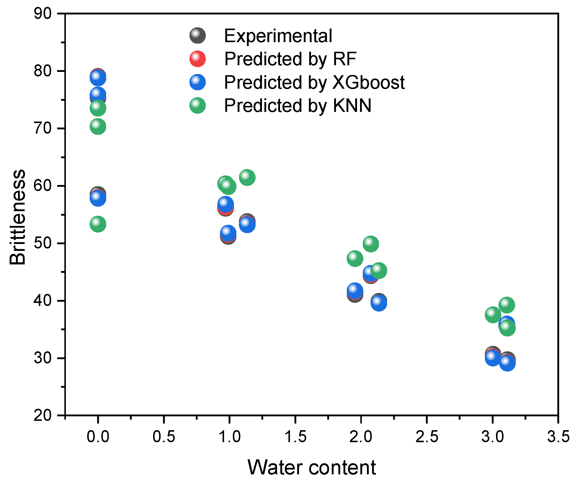
• Water content significantly influences the mechanical properties and brittleness of rocks. Studies indicate that, upon exposure to water, rocks experience a 41% reduction in brittleness, which lowers the likelihood of rock burst incidents. However, this interaction also compromises rock strength, increasing the risk of rock failure due to decreased overall strength.
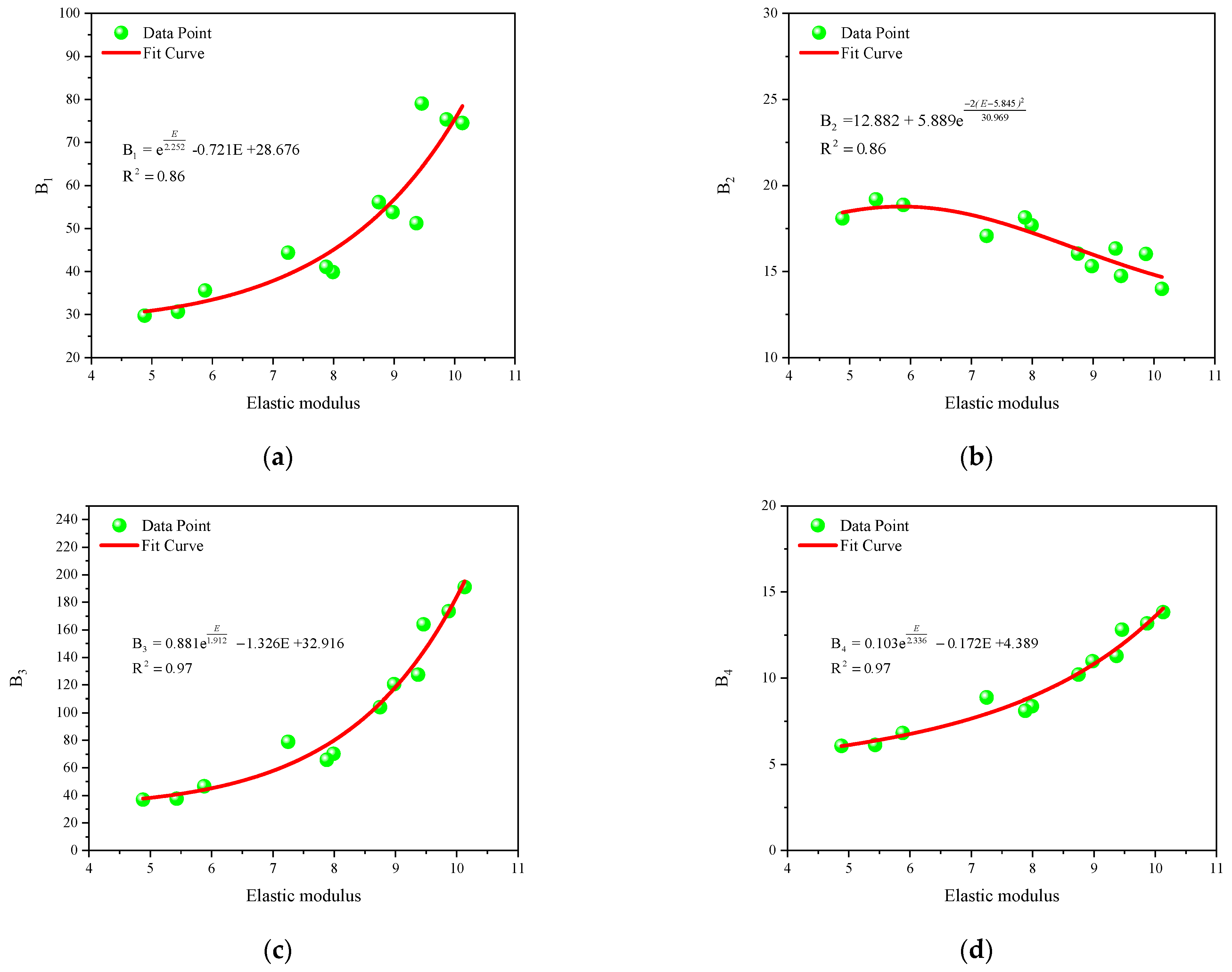
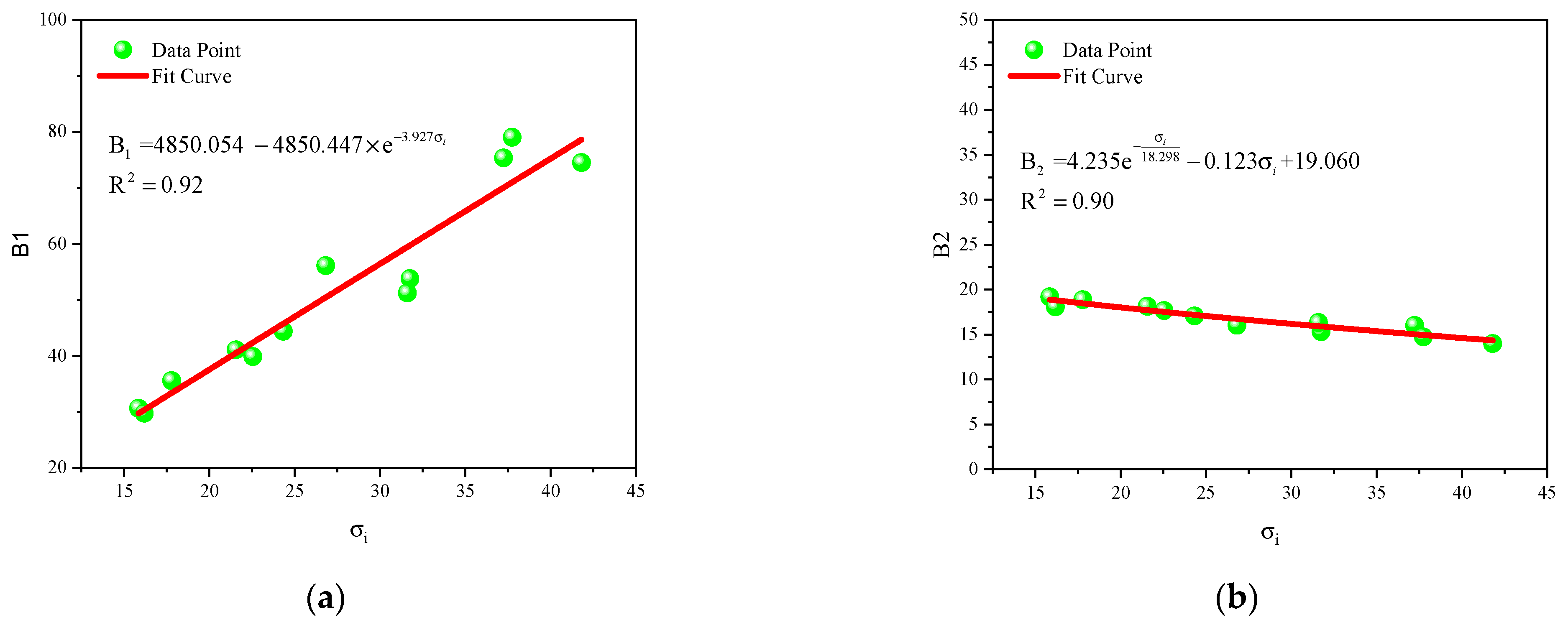
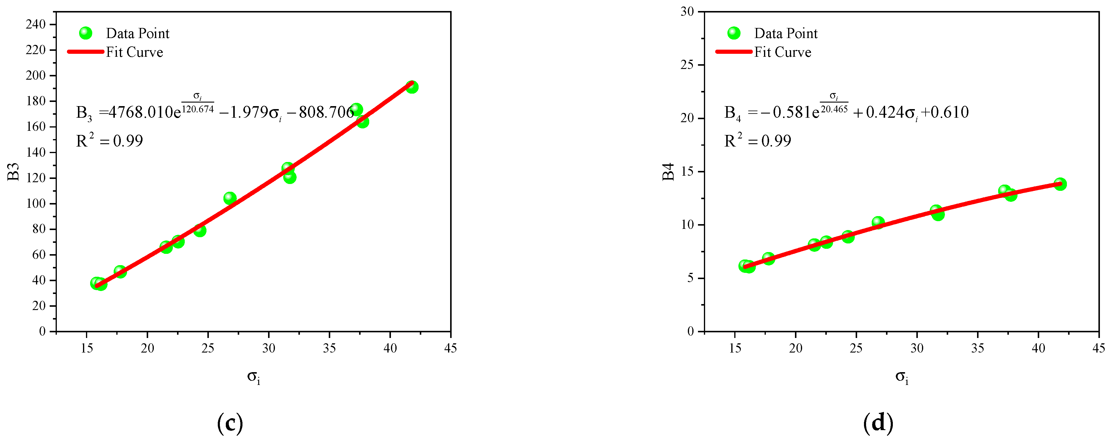
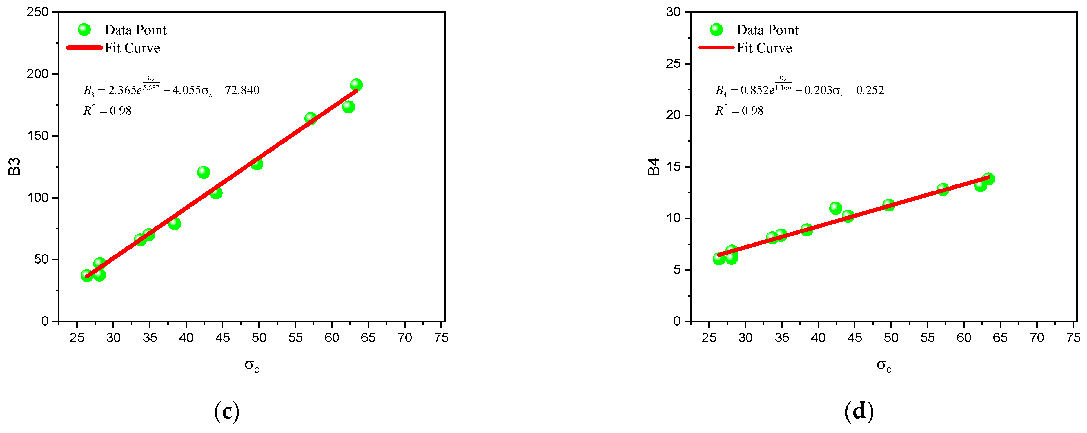
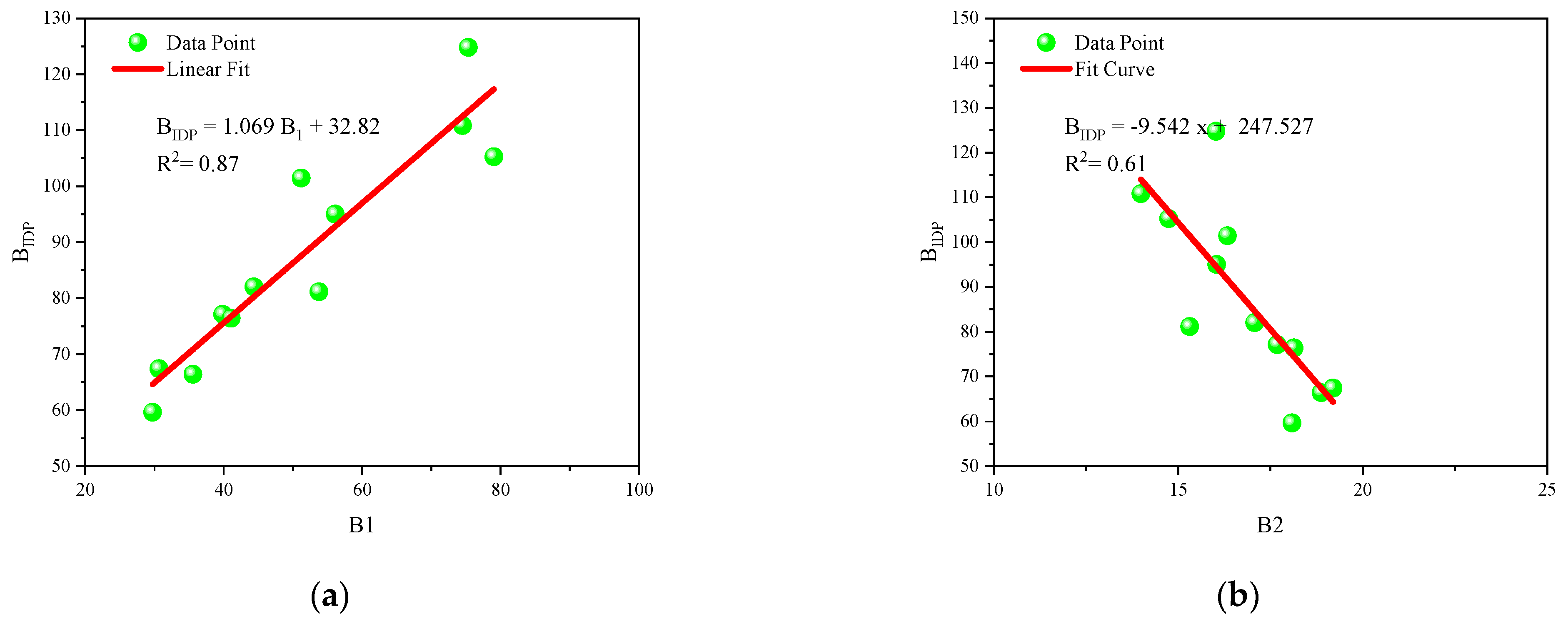
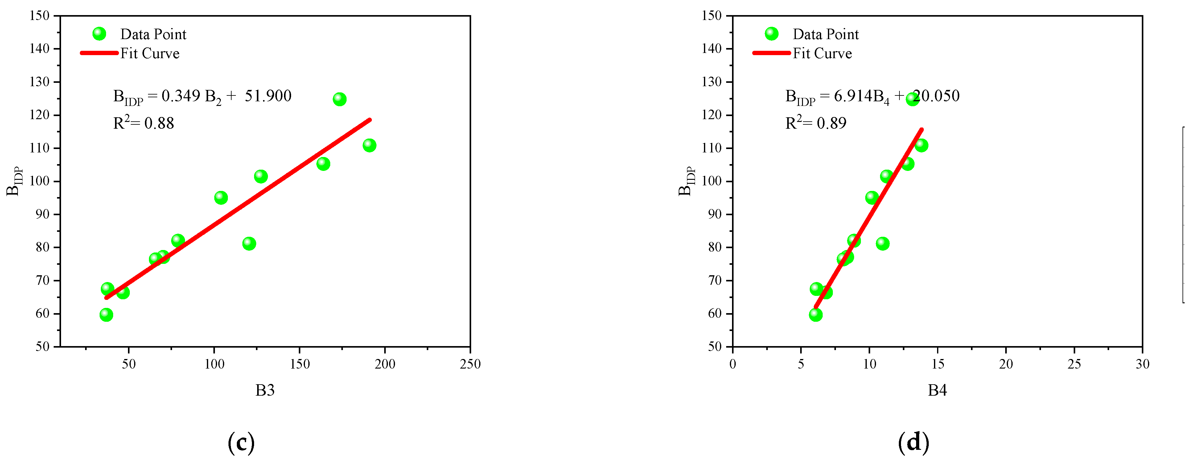
• The brittleness indices such as B₁, B₂, and B₄ show a positive linear exponential correlation, whereas B₂ shows a poor negative linear exponential correlation with crack initiation, elastic modulus, and crack damage stress. The proposed brittleness index B_IDP has a high linear correlation (R² > 0.88) with B₁, B₂, and B₄ and a poor negative linear correlation (R² > 0.88) with B₂. Therefore, the proposed index has high significance.
• The proposed brittleness considered elastic modulus, crack initiation, crack damage, and peak stress under different water contents, which truly reflected the brittleness intensity. The intensity decreases linearly exponentially (R² > 0.90) in the presence of water content.
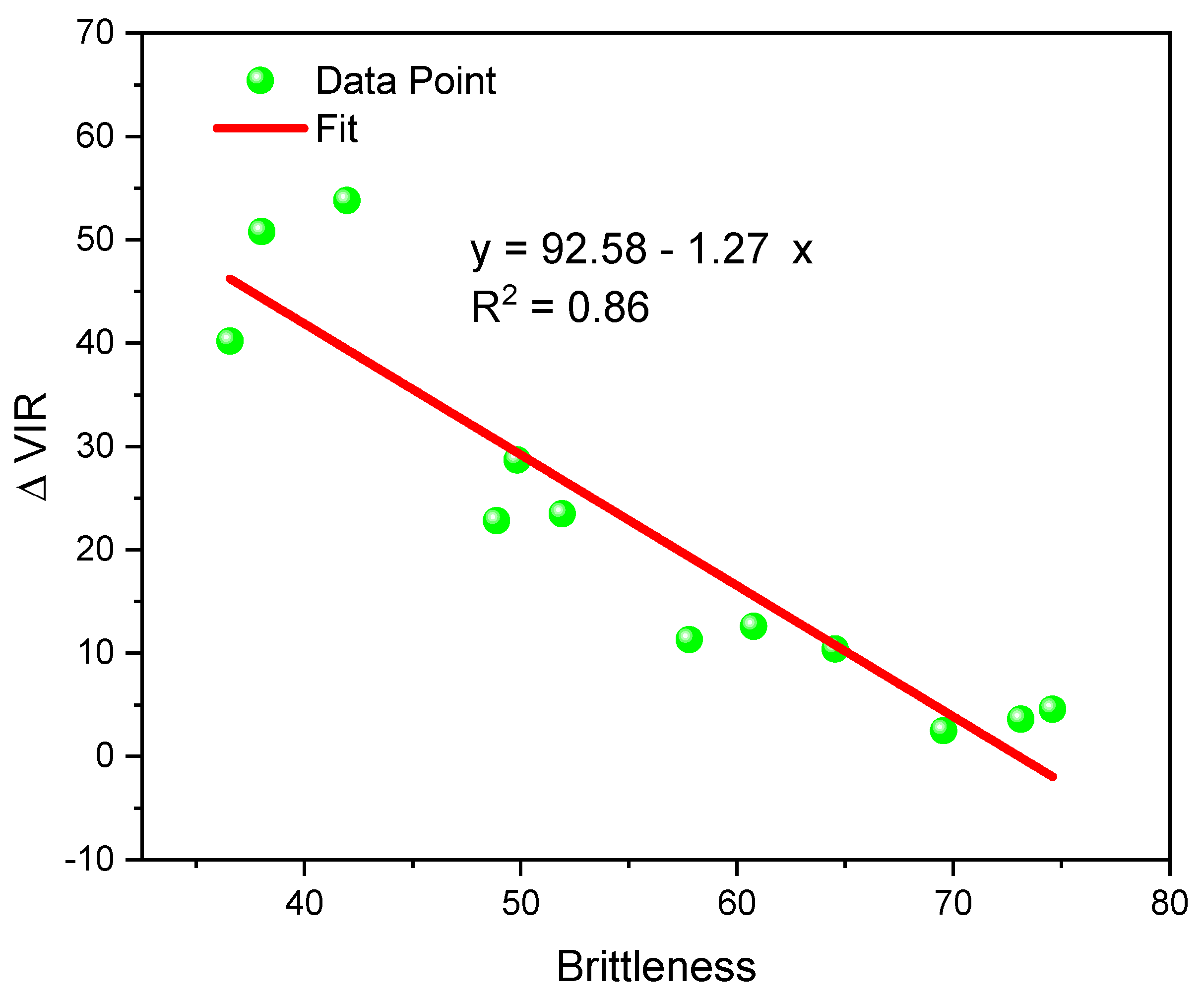
• During the peak stress phase, the rate of IRV rises in the presence of water but declines when the rock’s brittleness decreases. This implies that water presence impacts the IRV rate, while the rock’s brittleness affects its overall performance.
• To predict the proposed index, three different models, namely XGBoost, RF, and KNN, were utilized. By comparing their performance, it was found that both RF and XGBoost exhibit high prediction accuracy. Specifically, the RF model achieved an impressive R² value of 0.999, along with low values for RMSE (0.383), MSE (0.007), and MAE (0.002). Therefore, the RF model is recommended to be used effectively in the prediction of rock brittleness.
• These research findings establish a solid theoretical foundation for evaluating rock brittleness and predicting rock burst susceptibility. The incorporation of water conditions and the proposed index offer valuable insights for effectively assessing and mitigating the risks associated with rock burst incidents. These findings open up new avenues for further discussions and exploration in this field, paving the way for innovative approaches to rock burst prevention and management.

References

1. Meng, F.; Zhou, H.; Zhang, C.; Xu, R.; Lu, J. Evaluation methodology of brittleness of rock based on post-peak stress–strain curves. Rock Mech. Rock Eng. 2015, 48, 1787–1805. [Google Scholar] [CrossRef]
2. Zhao, Z.; Ali, E.; Wu, G.; Wang, X. Assessment of strain energy storage and rock brittleness indices of rockburst potential from microfabric characterizations. Am. J. Earth Sci. 2015, 2, 8. [Google Scholar]
3. Zhang, C.; Lu, J.; Chen, J.; Zhou, H.; Yang, F. Discussion on rock burst proneness indexes and their relation. Rock Soil Mech. 2017, 38, 1397–1404. [Google Scholar]
4. Zhang, L.; Cong, Y.; Meng, F.; Wang, Z.; Zhang, P.; Gao, S. Energy evolution analysis and failure criteria for rock under different stress paths. Acta Geotech. 2021, 16, 569–580. [Google Scholar] [CrossRef]
5. Gong, F.; Yan, J.; Li, X.; Luo, S. A peak-strength strain energy storage index for rock burst proneness of rock materials. Int. J. Rock Mech. Sci. 2019, 117, 76–89. [Google Scholar] [CrossRef]
6. Song, S.; Ren, T.; Dou, L.; Sun, J.; Yang, X.; Tan, L. Fracture features of brittle coal under uniaxial and cyclic compression loads. Int. J. Coal Sci. Technol. 2023, 10, 9. [Google Scholar] [CrossRef]
7. Ali, Z.; Karakus, M.; Nguyen, G.D.; Amrouch, K. Effect of loading rate and time delay on the tangent modulus method (TMM) in coal and coal measured rocks. Int. J. Coal Sci. Technol. 2022, 9, 81. [Google Scholar] [CrossRef]
8. Bai, Q.; Zhang, C.; Paul Young, R. Using true-triaxial stress path to simulate excavation-induced rock damage: A case study. Int. J. Coal Sci. Technol. 2022, 9, 49. [Google Scholar] [CrossRef]
9. Chen, Y.; Zuo, J.; Liu, D.; Li, Y.; Wang, Z. Experimental and numerical study of coal-rock bimaterial composite bodies under triaxial compression. Int. J. Coal Sci. Technol. 2021, 8, 908–924. [Google Scholar] [CrossRef]
10. Chi, X.; Yang, K.; Wei, Z. Breaking and mining-induced stress evolution of overlying strata in the working face of a steeply dipping coal seam. Int. J. Coal Sci. Technol. 2021, 8, 614–625. [Google Scholar] [CrossRef]
11. Feng, F.; Chen, S.; Zhao, X.; Li, D.; Wang, X.; Cui, J. Effects of external dynamic disturbances and structural plane on rock fracturing around deep underground cavern. Int. J. Coal Sci. Technol. 2022, 9, 15. [Google Scholar] [CrossRef]
12. He, S.; Qin, M.; Qiu, L.; Song, D.; Zhang, X. Early warning of coal dynamic disaster by precursor of AE and EMR “quiet period”. Int. J. Coal Sci. Technol. 2022, 9, 46. [Google Scholar] [CrossRef]
13. Huang, F.; Xiong, H.; Chen, S.; Lv, Z.; Huang, J.; Chang, Z.; Catani, F. Slope stability prediction based on a long short-term memory neural network: Comparisons with convolutional neural networks, support vector machines and random forest models. Int. J. Coal Sci. Technol. 2023, 10, 18. [Google Scholar] [CrossRef]
14. Li, Y.; Mitri, H.S. Determination of mining-induced stresses using diametral rock core deformations. Int. J. Coal Sci. Technol. 2022, 9, 80. [Google Scholar] [CrossRef]
15. Zhao, Y.; He, X.; Jiang, L.; Wang, Z.; Ning, J.; Sainoki, A. Influence analysis of complex crack geometric parameters on mechanical properties of soft rock. Int. J. Coal Sci. Technol. 2023, 10, 78. [Google Scholar] [CrossRef]
16. Xu, L.; Fan, C.; Luo, M.; Li, S.; Han, J.; Fu, X.; Xiao, B. Elimination mechanism of coal and gas outburst based on geo-dynamic system with stress–damage–seepage interactions. Int. J. Coal Sci. Technol. 2023, 10, 74. [Google Scholar] [CrossRef]
17. Soleimani, F.; Si, G.; Roshan, H.; Zhang, J. Numerical modelling of gas outburst from coal: A review from control parameters to the initiation process. Int. J. Coal Sci. Technol. 2023, 10, 81. [Google Scholar] [CrossRef]
18. Munoz, H.; Taheri, A.; Chanda, E. Rock drilling performance evaluation by an energy dissipation based rock brittleness index. Rock Mech. Rock Eng. 2016, 49, 3343–3355. [Google Scholar] [CrossRef]
19. Meng, F.; Wong, L.N.Y.; Zhou, H. Rock brittleness indices and their applications to different fields of rock engineering: A review. J. Rock Mech. Geotech. Eng. 2021, 13, 221–247. [Google Scholar] [CrossRef]
20. Liang, L.; Liu, X.; Xiong, J.; Wu, T.; Ding, Y. New model to evaluate the Brittleness in shale formation. In International Geophysical Conference, Qingdao, China, 17–20 April 2017; SEG Global Meeting Abstracts; Society of Exploration Geophysicists and Chinese Petroleum Society: Houston, TX, USA, 2017; pp. 1248–1251. [Google Scholar]
21. Gong, X.; Sun, C.C. A new tablet brittleness index. Eur. J. Pharm. Biopharm. 2015, 93, 260–266. [Google Scholar] [CrossRef]
22. Wang, Y.; Li, X.; Wu, Y.; Ben, Y.; Li, S.; He, J.; Zhang, B. Research on relationship between crack initiation stress level and brittleness indices for brittle rocks. Chin. J. Rock Mech. Eng. 2014, 33, 264–275. [Google Scholar]
23. Bishop, A. Progressive failure-with special reference to the mechanism causing it. In Proceedings of the Geotechnical Conference Oslo 1967 on Shear Strength Properties of Natural Soils and Rocks; Norwegian Geotechnical Institute: Oslo, Norway, 1967; pp. 142–150. [Google Scholar]
24. Baud, P.; Zhu, W.; Wong, T.F. Failure mode and weakening effect of water on sandstone. J. Geophys. Res. Solid Earth 2000, 105, 16371–16389. [Google Scholar] [CrossRef]
25. Liu, X.; Yang, C.; Yu, J. The influence of moisture content on the time-dependent characteristics of rock material and its application to the construction of a tunnel portal. Adv. Mater. Sci. Eng. 2015, 2015, 725162. [Google Scholar] [CrossRef]
26. Nicolas, A.; Fortin, J.; Regnet, J.; Dimanov, A.; Guéguen, Y. Brittle and semi-brittle behaviours of a carbonate rock: Influence of water and temperature. Geophys. J. Int. 2016, 206, 438–456. [Google Scholar] [CrossRef]
27. Li, Y.; Yang, R.; Fang, S.; Lin, H.; Lu, S.; Zhu, Y.; Wang, M. Failure analysis and control measures of deep roadway with composite roof: A case study. Int. J. Coal Sci. Technol. 2022, 9, 2. [Google Scholar] [CrossRef]
28. Liu, B.; Zhao, Y.; Zhang, C.; Zhou, J.; Li, Y.; Sun, Z. Characteristic strength and acoustic emission properties of weakly cemented sandstone at different depths under uniaxial compression. Int. J. Coal Sci. Technol. 2021, 8, 1288–1301. [Google Scholar] [CrossRef]
29. Liu, T.; Lin, B.; Fu, X.; Liu, A. Mechanical criterion for coal and gas outburst: A perspective from multiphysics coupling. Int. J. Coal Sci. Technol. 2021, 8, 1423–1435. [Google Scholar] [CrossRef]
30. Małkowski, P.; Niedbalski, Z.; Balarabe, T. A statistical analysis of geomechanical data and its effect on rock mass numerical modeling: A case study. Int. J. Coal Sci. Technol. 2021, 8, 312–323. [Google Scholar] [CrossRef]
31. Pang, Y.; Wang, H.; Lou, J.; Chai, H. Longwall face roof disaster prediction algorithm based on data model driving. Int. J. Coal Sci. Technol. 2022, 9, 11. [Google Scholar] [CrossRef]
32. Wang, G.; Ren, H.; Zhao, G.; Zhang, D.; Wen, Z.; Meng, L.; Gong, S. Research and practice of intelligent coal mine technology systems in China. Int. J. Coal Sci. Technol. 2022, 9, 24. [Google Scholar] [CrossRef]
33. Wei, C.; Zhang, C.; Canbulat, I.; Song, Z.; Dai, L. A review of investigations on ground support requirements in coal burst-prone mines. Int. J. Coal Sci. Technol. 2022, 9, 13. [Google Scholar] [CrossRef]
34. Khan, N.M.; Ma, L.; Cao, K.; Hussain, S.; Liu, W.; Xu, Y.; Yuan, Q.; Gu, J. Prediction of an early failure point using infrared radiation characteristics and energy evolution for sandstone with different water contents. Bull. Eng. Geol. Environ. 2021, 80, 6913–6936. [Google Scholar] [CrossRef]
35. Song, Z.; Zhang, J.; Wu, S. Energy Dissipation and Fracture Mechanism of Layered Sandstones under Coupled Hydro-Mechanical Unloading. Processes 2023, 11, 2041. [Google Scholar] [CrossRef]
36. Wasantha, P.L.P.; Ranjith, P.G. Water-weakening behavior of Hawkesbury sandstone in brittle regime. Eng. Geol. 2014, 178, 91–101. [Google Scholar] [CrossRef]
37. Ortlepp, W.D. Rock Fracture and Rockbursts: An Illustrative Study; South African Institute of Mining and Metallurgy: Johannesburg, South Africa, 1997; Volume 9. [Google Scholar]
38. Fowkes, N. Rockbursts mud and plastic. In Proceedings of the 19th International Congress on Modelling and Simulation, Modelling and Simulation Society of Australia and New Zealand, Perth, Australia, 12–16 December 2011; pp. 12–16. [Google Scholar]
39. Gong, Q.M.; Yin, L.J.; Wu, S.Y.; Zhao, J.; Ting, Y. Rock burst and slabbing failure and its influence on TBM excavation at headrace tunnels in Jinping II hydropower station. Eng. Geol. 2012, 124, 98–108. [Google Scholar] [CrossRef]
40. Wu, H.; Chen, Y.; Lv, H.; Xie, Q.; Chen, Y.; Gu, J. Stability analysis of rib pillars in highwall mining under dynamic and static loads in open-pit coal mine. Int. J. Coal Sci. Technol. 2022, 9, 38. [Google Scholar] [CrossRef]
41. Wu, H.; Ju, Y.; Han, X.; Ren, Z.; Sun, Y.; Zhang, Y.; Han, T. Size effects in the uniaxial compressive properties of 3D printed models of rocks: An experimental investigation. Int. J. Coal Sci. Technol. 2022, 9, 83. [Google Scholar] [CrossRef]
42. Wu, R.; Zhang, P.; Kulatilake, P.H.S.W.; Luo, H.; He, Q. Stress and deformation analysis of gob-side pre-backfill driving procedure of longwall mining: A case study. Int. J. Coal Sci. Technol. 2021, 8, 1351–1370. [Google Scholar] [CrossRef]
43. Xie, J.; Ge, F.; Cui, T.; Wang, X. A virtual test and evaluation method for fully mechanized mining production system with different smart levels. Int. J. Coal Sci. Technol. 2022, 9, 41. [Google Scholar] [CrossRef]
44. Xue, D.; Lu, L.; Zhou, J.; Lu, L.; Liu, Y. Cluster modeling of the short-range correlation of acoustically emitted scattering signals. Int. J. Coal Sci. Technol. 2021, 8, 575–589. [Google Scholar] [CrossRef]
45. Yang, D.; Ning, Z.; Li, Y.; Lv, Z.; Qiao, Y. In situ stress measurement and analysis of the stress accumulation levels in coal mines in the northern Ordos Basin, China. Int. J. Coal Sci. Technol. 2021, 8, 1316–1335. [Google Scholar] [CrossRef]
46. Yuan, Y.; Wang, S.; Wang, W.; Zhu, C. Numerical simulation of coal wall cutting and lump coal formation in a fully mechanized mining face. Int. J. Coal Sci. Technol. 2021, 8, 1371–1383. [Google Scholar] [CrossRef]
47. Zhang, S.; Lu, L.; Wang, Z.; Wang, S. A physical model study of surrounding rock failure near a fault under the influence of footwall coal mining. Int. J. Coal Sci. Technol. 2021, 8, 626–640. [Google Scholar] [CrossRef]
48. Zhou, J.; Lin, H.; Jin, H.; Li, S.; Yan, Z.; Huang, S. Cooperative prediction method of gas emission from mining face based on feature selection and machine learning. Int. J. Coal Sci. Technol. 2022, 9, 51. [Google Scholar] [CrossRef]
49. Pappalardo, G.; Mineo, S.; Zampelli, S.P.; Cubito, A.; Calcaterra, D. InfraRed Thermography proposed for the estimation of the Cooling Rate Index in the remote survey of rock masses. Int. J. Rock Mech. Min. Sci. 2016, 83, 182–196. [Google Scholar] [CrossRef]
50. Cao, K.; Ma, L.; Wu, Y.; Khan, N.; Yang, J. Using the characteristics of infrared radiation during the process of strain energy evolution in saturated rock as a precursor for violent failure. Infrared Phys. Technol. 2020, 109, 103406. [Google Scholar] [CrossRef]
51. Sun, X.; Xu, H.; He, M.; Zhang, F. Experimental investigation of the occurrence of rockburst in a rock specimen through infrared thermography and acoustic emission. Int. J. Rock Mech. Min. Sci. 2017, 93, 9. [Google Scholar] [CrossRef]
52. Ma, L.; Sun, H.; Zhang, Y.; Zhou, T.; Li, K.; Guo, J. Characteristics of infrared radiation of coal specimens under uniaxial loading. Rock Mech. Rock Eng. 2016, 49, 1567–1572. [Google Scholar] [CrossRef]
53. Hou, L.; Ma, L.; Cao, K.; Muhammad Khan, N.; Feng, X.; Zhang, Z.; Cao, A.; Wang, D.; Wang, X. Analysis of fracture characteristics of saturated sandstone based on infrared radiation variance. Phys. Chem. Earth Parts A/B/C 2024, 133, 103517. [Google Scholar] [CrossRef]
54. Cao, K.; Dong, F.; Liu, W.; Khan, N.M.; Cui, R.; Li, X.; Hussain, S.; Alarifi, S.S.; Niu, D.J.I.P. Infrared radiation denoising model of “sub-region-Gaussian kernel function” in the process of sandstone loading and fracture. Infrared Phys. Technol. 2023, 129, 104583. [Google Scholar] [CrossRef]
55. Hou, L.; Cao, K.; Muhammad Khan, N.; Jahed Armaghani, D.; SAlarifi, S.; Hussain, S.; Ali, M. Precursory Analysis of Water-Bearing Rock Fracture Based on The Proportion of Dissipated Energy. Sustainability 2023, 15, 1769. [Google Scholar] [CrossRef]
56. Muhammad Khan, N.; Ma, L.; Feroze, T.; Wang, D.; Cao, K.; Gao, Q.; Wang, H.; Hussain, S.; Zhang, Z.; Alarifi, S.S. Investigating average infrared radiation temperature characteristics during shear and tensile cracks in sandstone under different water contents. Infrared Phys. Technol. 2023, 135, 104968. [Google Scholar] [CrossRef]
57. Cao, K.; Dong, F.; Ma, L.; Khan, N.M.; Alarifi, S.S.; Hussain, S.; Armaghani, D.J. Infrared radiation constitutive model of sandstone during loading fracture. Infrared Phys. Technol. 2023, 133, 104755. [Google Scholar] [CrossRef]
58. Cao, K.; Dong, F.; Yu, Y.; Khan, N.M.; Hussain, S.; Alarifi, S.S. Infrared radiation response mechanism of sandstone during loading and fracture process. Theor. Appl. Fract. Mech. 2023, 126, 103974. [Google Scholar] [CrossRef]
59. Wu, L.; Liu, S.; Wu, Y.; Wang, C. Precursors for rock fracturing and failure—Part II: IRR T-Curve abnormalities. Int. J. Rock Mech. Min. Sci. 2006, 43, 483–493. [Google Scholar] [CrossRef]
60. Liu, S.; Wu, L.; Wu, Y. Infrared radiation of rock at failure. Int. J. Rock Mech. Min. Sci. 2006, 43, 972–979. [Google Scholar] [CrossRef]
61. Ma, L.; Zhang, Y. An Experimental Study on Infrared Radiation Characteristics of Sandstone Samples Under Uniaxial Loading. Rock Mech. Rock Eng. 2019, 52, 3493–3500. [Google Scholar] [CrossRef]
62. Ma, L.; Khan, N.M.; Cao, K.; Rehman, H.; Salman, S.; Rehman, F.U. Prediction of Sandstone Dilatancy Point in Different Water Contents Using Infrared Radiation Characteristic: Experimental and Machine Learning Approaches. Lithosphere 2022, 2021, 3243070. [Google Scholar] [CrossRef]
63. Wei, Y.; Li, Z.; Kong, X.; Zhang, Z.; Cheng, F.; Zheng, X.; Wang, C. The precursory information of acoustic emission during sandstone loading based on critical slowing down theory. J. Geophys. Eng. 2018, 15, 2150–2158. [Google Scholar] [CrossRef]
64. Sharma, L.K.; Singh, T.N. Regression-based models for the prediction of unconfined compressive strength of artificially structured soil. Eng. Comput. 2018, 34, 175–186. [Google Scholar] [CrossRef]
65. Huang, B.; Liu, J. The effect of loading rate on the behavior of samples composed of coal and rock. Int. J. Rock Mech. Min. Sci. 2013, 61, 23–30. [Google Scholar] [CrossRef]
66. Breiman, L. Random forests. Mach. Learn. 2001, 45, 5–32. [Google Scholar] [CrossRef]
67. Ogunkunle, T.F.; Okoro, E.E.; Rotimi, O.J.; Igbinedion, P.; Olatunji, D.I. Artificial intelligence model for predicting geomechanical characteristics using easy-to-acquire offset logs without deploying logging tools. Petroleum 2022, 8, 192–203. [Google Scholar] [CrossRef]
68. Qi, C.; Fourie, A.; Du, X.; Tang, X. Prediction of open stope hangingwall stability using random forests. Nat. Hazards 2018, 92, 1179–1197. [Google Scholar] [CrossRef]
69. Zhou, J.; Li, X.; Mitri, H.S. Comparative performance of six supervised learning methods for the development of models of hard rock pillar stability prediction. Nat. Hazards 2015, 79, 291–316. [Google Scholar] [CrossRef]
70. Qi, Q.; Yue, X.; Duo, X.; Xu, Z.; Li, Z. Spatial prediction of soil organic carbon in coal mining subsidence areas based on RBF neural network. Int. J. Coal Sci. Technol. 2023, 10, 30. [Google Scholar] [CrossRef]
71. Khan, N.M.; Cao, K.; Yuan, Q.; Bin Mohd Hashim, M.H.; Rehman, H.; Hussain, S.; Emad, M.Z.; Ullah, B.; Shah, K.S.; Khan, S. Application of machine learning and multivariate statistics to predict uniaxial compressive strength and static Young’s modulus using physical properties under different thermal conditions. Sustainability 2022, 14, 9901. [Google Scholar] [CrossRef]
72. Yang, Z.; Wu, Y.; Zhou, Y.; Tang, H.; Fu, S. Assessment of Machine Learning Models for the Prediction of Rate-Dependent Compressive Strength of Rocks. Minerals 2022, 12, 731. [Google Scholar] [CrossRef]
73. Wu, X.; Kumar, V.; Ross Quinlan, J.; Ghosh, J.; Yang, Q.; Motoda, H.; McLachlan, G.J.; Ng, A.; Liu, B.; Yu, P.S.; et al. Top 10 algorithms in data mining. Knowl. Inf. Syst. 2008, 14, 1–37. [Google Scholar] [CrossRef]
74. Akbulut, Y.; Sengur, A.; Guo, Y.; Smarandache, F. NS-k-NN: Neutrosophic Set-Based k-Nearest Neighbors Classifier. Symmetry 2017, 9, 179. [Google Scholar] [CrossRef]
75. Qian, Y.; Zhou, W.; Yan, J.; Li, W.; Han, L. Comparing Machine Learning Classifiers for Object-Based Land Cover Classification Using Very High Resolution Imagery. Remote Sens. 2015, 7, 153–168. [Google Scholar] [CrossRef]
76. Chen, T.; Guestrin, C. Xgboost: A scalable tree boosting system. In Proceedings of the 22nd ACM SIGKDD International Conference on Knowledge Discovery and Data Mining, San Francisco, CA, USA, 13–17 August 2016; pp. 785–794. [Google Scholar]
77. Zhu, X.; Chu, J.; Wang, K.; Wu, S.; Yan, W.; Chiam, K. Prediction of rockhead using a hybrid N-XGBoost machine learning framework. J. Rock Mech. Geotech. Eng. 2021, 13, 1231–1245. [Google Scholar] [CrossRef]
78. Liu, X.; Chen, H.; Liu, B.; Wang, S.; Liu, Q.; Luo, Y.; Luo, J. Experimental and numerical investigation on failure characteristics and mechanism of coal with different water contents. Int. J. Coal Sci. Technol. 2023, 10, 49. [Google Scholar] [CrossRef]
79. Ma, L.; Muhammad Khan, N.; Feroze, T.; Sazid, M.; Cao, K.; Hussain, S.; Gao, Q.; Alarifi, S.S.; Wang, H. Prediction of rock loading stages using average infrared radiation temperature under shear and uniaxial loading. Infrared Phys. Technol. 2024, 136, 105084. [Google Scholar] [CrossRef]
80. Zhao, Y.; Zhang, L.; Wang, W.; Tang, J.; Lin, H.; Wan, W. Transient pulse test and morphological analysis of single rock fractures. Int. J. Rock Mech. Min. Sci. 2017, 91, 139–154. [Google Scholar] [CrossRef]
81. Liu, X.; Fu, Y.; Zheng, Y.; Liang, N. A review on deterioration of rock caused by water-rock interaction. Chin. J. Undergr. Space Eng. 2012, 8, 77–82. [Google Scholar]
82. Cao, K.; Ma, L.; Zhang, D.; Lai, X.; Zhang, Z.; Khan, N.M. An experimental study of infrared radiation characteristics of sandstone in dilatancy process. Int. J. Rock Mech. Min. Sci. 2020, 136, 104503. [Google Scholar] [CrossRef]
83. Liashchynskyi, P.; Liashchynskyi, P. Grid search, random search, genetic algorithm: A big comparison for NAS. arXiv 2019, arXiv:1912.06059. [Google Scholar]
84. Yang, H.Q.; Zeng, Y.Y.; Lan, Y.F.; Zhou, X.P. Analysis of the excavation damaged zone around a tunnel accounting for geostress and unloading. Int. J. Rock Mech. Min. Sci. 2014, 69, 59–66. [Google Scholar] [CrossRef]
85. Chai, C.; Ling, S.; Wu, X.; Hu, T.; Sun, D. Characteristics of the In Situ Stress Field and Engineering Effect along the Lijiang to Shangri-La Railway on the Southeastern Tibetan Plateau, China. Adv. Civ. Eng. 2021, 2021, 6652790. [Google Scholar] [CrossRef]
86. Deng, D.; Wang, H.; Xie, L.; Wang, Z.; Song, J. Experimental study on the interrelation of multiple mechanical parameters in overburden rock caving process during coal mining in longwall panel. Int. J. Coal Sci. Technol. 2023, 10, 47. [Google Scholar] [CrossRef]
87. Tan, Y.; Ma, Q.; Liu, X.; Liu, X.; Elsworth, D.; Qian, R.; Shang, J. Study on the disaster caused by the linkage failure of the residual coal pillar and rock stratum during multiple coal seam mining: Mechanism of progressive and dynamic failure. Int. J. Coal Sci. Technol. 2023, 10, 45. [Google Scholar] [CrossRef]
88. Leśniak, G.; Brunner, D.J.; Topór, T.; Słota-Valim, M.; Cicha-Szot, R.; Jura, B.; Skiba, J.; Przystolik, A.; Lyddall, B.; Plonka, G. Correction to: Application of long-reach directional drilling boreholes for gas drainage of adjacent seams in coal mines with severe geological conditions. Int. J. Coal Sci. Technol. 2023, 10, 39. [Google Scholar] [CrossRef]
89. Luo, J.; Li, Y.; Meng, X.; Guo, Q.; Zhao, G. Influence of coupling mechanism of loose layer and fault on multi-physical fields in mining areas. Int. J. Coal Sci. Technol. 2023, 10, 86. [Google Scholar] [CrossRef]
Figure 1. Experimental system for infrared radiation observation of sandstone under different loading rates.
Water 16 00143 g001
Figure 2. Basic Structure of RFR.
Water 16 00143 g002
Figure 3. XGBoost model’s general structure.
Water 16 00143 g003
Figure 4. Heat map of dependent and independent variable.
Water 16 00143 g004
Figure 5. Box plot of input dataset: (a) the data without being normalized, (b) normalized data, (c) the normalized data without outlier.
Water 16 00143 g005
Figure 6. Stress–strain curve: (a) different water content; (b) loading stages.
Water 16 00143 g006
Figure 7. Stiffness–stress and stress–strain curve of sandstone.
Water 16 00143 g007
Figure 8. Relationship of different brittleness indices and water content: (a) B1; (b) B2; (c) B3; and (d) B4.
Water 16 00143 g008
Figure 9. Relationship of different brittleness indices and elastic modulus: (a) B1; (b) B2; (c) B3; and (d) B4.
Water 16 00143 g009
Figure 10. Relationship of different brittleness indices and crack initiation stress: (a) B1; (b) B2; (c) B3; and (d) B4.
Water 16 00143 g010aWater 16 00143 g010b
Figure 11. Relationship of different brittleness indices and crack damage stress: (a) B1; (b) B2; (c) B3; and (d) B4.
Water 16 00143 g011aWater 16 00143 g011b
Figure 12. Relationship between proposed and existing brittleness index. (a) B1; (b) B2; (c) B3; and (d) B4.
Water 16 00143 g012aWater 16 00143 g012b
Figure 13. Relation between proposed brittleness index and VIR.
Water 16 00143 g013
Figure 14. IRV and stress for different water content: (a) dry; (bd) saturated.
Water 16 00143 g014
Figure 15. Flowchart of proposed model for brittleness index.
Water 16 00143 g015
Figure 16. Actual and predicted stress–strain curve in different water content conditions: (a) dry; (b) 0.971%; (c) 2.075%; (d) 3.109%.
Water 16 00143 g016
Figure 17. Radar plot for comparison of XGBoost, RF, and KNN.
Water 16 00143 g017
Figure 18. Actual and predicted values of brittleness for different models.
Water 16 00143 g018