Spatiotemporal Evolution and Attribution Analysis of Water Yield in the Xiangjiang River Basin (XRB) Based on the InVEST Model

Abstract

As a result of climate change and human activities, water resources in the Xiangjiang River Basin (XRB) are subject to seasonal and regional shortages. However, previous studies have lacked assessment of the spatiotemporal evolution of water yield in the XRB at seasonal and monthly scales and quantitative analysis of the driving forces of climate change and land use on water-yield change. Quantitative evaluation of water yield in the XRB is of great significance for optimizing water-resource planning and allocation and maintaining ecological balance in the basin. In this paper, the seasonal water-yield InVEST model and modified Morris sensitivity analysis were combined to study the characteristics of monthly water yield in the XRB. Seventeen attributes were identified using the Budyko framework. The results show that: (1) the water yield of the XRB showed an increase trend from northeast to southwest from 2006 to 2020; (2) the transfer-in of unused land, grassland, woodland and farmland as well as the transfer-out of water and construction land have positive effects on the increase in water yield, and the change to construction land has the greatest impact on water yield; (3) water yield is positively correlated with NDVI and precipitation and negatively correlated with potential evapotranspiration; (4) climate change and land-use change contributed to water-yield changes of 67.08% and 32.92%, respectively.

1. Introduction

Water resources are not only indispensable resources for human survival, but also important conditions for maintaining and ensuring the sustainable development of regional economies and ecosystems [1,2]. The spatial distribution of various regional economic elements (population, agriculture, industry, etc.) is limited by the distribution of water resources to a certain extent. Due to the human needs of living and production increasing with the acceleration of urbanization, the demand for water resources is increasing rapidly and accordingly. At the same time, due to the serious water pollution and water waste caused by human activities, the problem of water shortage has arisen in some areas [3,4,5]. Therefore, studying the spatiotemporal distribution of and variation in water yield and probing the driving factors is of great importance for the rational development and utilization of regional water resources [6]. Water yield, affected by various factors, such as precipitation, soil texture, soil depth, evapotranspiration, land use [7] and plant root depth, is therefore a complex issue.

Currently, many hydrological models are used to study water yield, including the ARIES model, the InVEST model [8] and the MIMES model, etc. Among them, the InVEST model has been successfully studied by many scholars, such as Polasky [9], Mansoor [10] and Marquèsa [11], to evaluate water-yield and ecosystem services in domestic and foreign contexts. With the continuous improvement of the application of the InVEST model, it can be found from the existing research results that scholars can not only evaluate water yield, but also conduct comprehensive, dynamic and visual evaluations of water yield in different scenarios. For example, Gao simulated spatiotemporal changes in water yield in the basin of the Guishui River based on different land-use scenarios, and the relationships between different ecosystem services were analyzed [12]. Wang JX [13] analyzed the degree to which land use influenced water yield based on different scenarios for ten river basins in China in the future. Wei JP et al. [14] designed three future scenarios based on climate change and land-use change and discussed their impacts on water yield in the Shule River Basin. We can not only use the InVEST model to evaluate spatiotemporal variation characteristics, but also the impact of different influencing factors on water yield in combination with other technical means [15,16]. For example, Tian Hu et al. discussed the relationship between soil erosion control (SEC) and water yield (WY), summarizing that SEC and WY presented a positive linear correlation on a watershed scale over time [17]. Zhang et al. analyzed the Yangtze River Basin and concluded that the water yield in the Yangtze River Basin was closely related to the average annual precipitation and the urban area in particular [18].

Although the InVEST water-yield model is widely used at present, research on spatiotemporal patterns of water yield is mostly limited to the annual scale, and there is a lack of research at the seasonal and monthly scales. In addition, research on the factors influencing water yield mostly lacks quantitative analysis [19], frequently being limited to qualitative analysis. The XRB, as one of the largest economic and cultural regions in Hunan Province, is in urgent need of ecological environmental protection. In recent years, the water resources of the Xiangjiang River have been in short supply during the dry season, resulting in low river water levels, and the ecological problems have become more and more serious. On the other hand, droughts and floods often occur in the XRB, where water resources are unevenly distributed in time and space [20]. The main purpose of this study is to (1) extend the time scale of water-yield assessment from annual to monthly and seasonal scales and (2) quantitatively analyze the extent to which the two factors of climate change and land-use change affect water yield using attribution analysis. The research results can provide scientific support for regional water-resource planning and management and reservoir construction and are of great significance for improving and regulating water-resource conservation capacities and maintaining regional sustainable development.

2. Materials and Methods

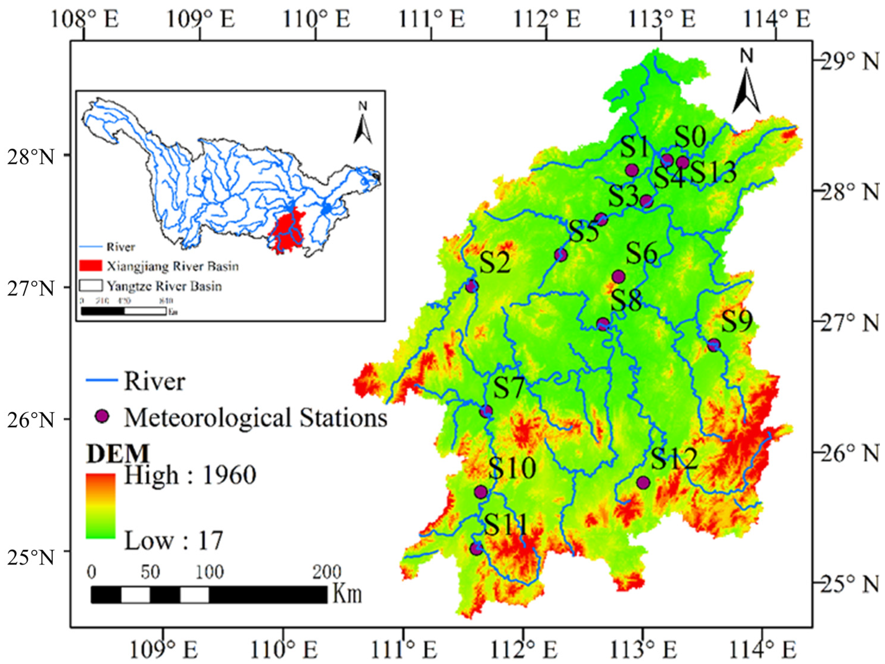
2.1. Research Area

The Xiangjiang River, a tributary of the Yangtze River, is also the river with the widest basin area in the Dongting Lake system (Figure 1). The total length of the Xiangjiang River from its source to the Haohe Estuary is 856 km, with a watershed area of 94,300 km², 85,383 km² of which is in Hunan Province, accounting for 90% of the total basin and about 40% of the total area of Hunan Province [21].

2.2. Data Sources

Meteorological data, elevation (DEM) data, land-use data, soil data, normalized vegetation index (NDVI) and actual surface-water yield are shown in

Table 1. Data information and sources.

Data	Data Brief	Data Sources
Meteorological data	Precipitation, maximum temperature, minimum temperature, atmospheric radiation, rainfall days	China Meteorological Science Data Network
Elevation (DEM) data	30 m resolution	Geospatial Data Cloud
Land-use data	30 m resolution	Landsat Remote Sensing Image Data
Soil data	Soil texture, soil type	Cold and Arid Region Scientific Data Center
Normalized vegetation index (NDVI)	1 km resolution	Resource and Environmental Science and Data Center, Chinese Academy of Sciences
Actual surface-water yield	2006–2020 year	Hunan Province Water Resources Bulletin

.

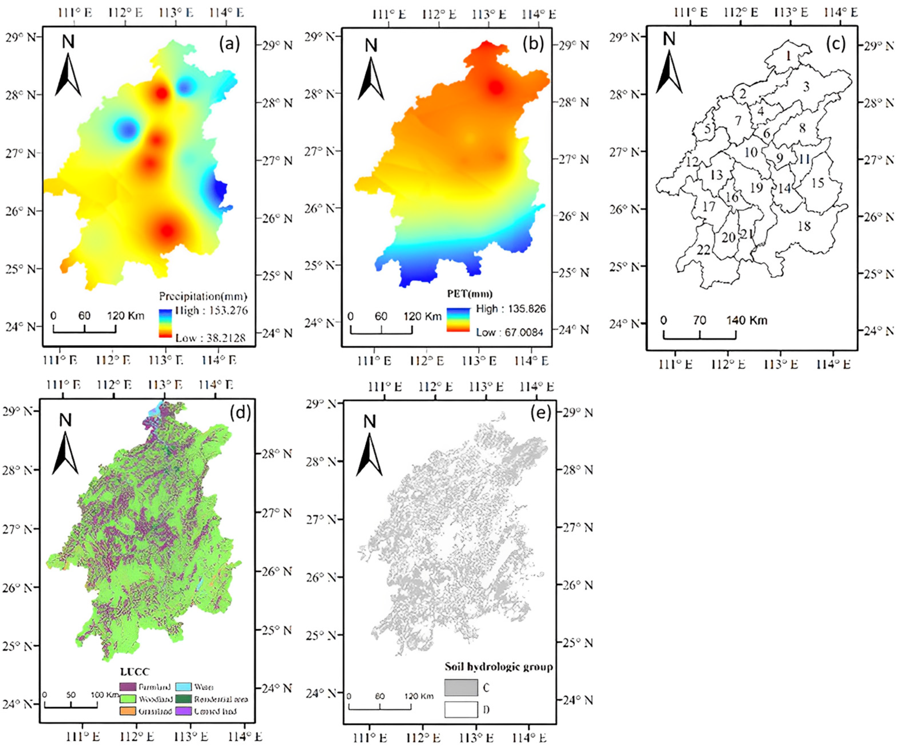
2.2.1. Meteorological Data

We collected daily rainfall data from 2006 to 2020 from 14 meteorological stations within the XRB and processed them into monthly rainfall data through accumulation. These station data were then converted into raster-based rainfall data using the Kriging interpolation method and ArcGIS software. Figure 2a shows rainfall in the XRB in January of 2006 as an example.

Potential evapotranspiration generally is determined by the Penman–Monteith (PM) formula, but due to the many parameters needed, its use is limited by data [22,23]. Therefore, the Modified Hargreaves method recommended by the InVEST model was used for the calculation of potential evapotranspiration in this study. The Modified Hargreaves calculations were based on daily rainfall data, maximum temperature data, minimum temperature data and solar radiation data obtained from 14 meteorological stations around the XRB from 2006 to 2020, and monthly potential evapotranspiration results were obtained through cumulative processing. After processing, the meteorological station distribution map was established in ArcGIS, and the spatial distribution grid map of monthly potential evapotranspiration from January to December between 2006 and 2020 was obtained by spatial interpolation using Kriging interpolation. An example of potential evapotranspiration (for January 2006) is shown in Figure 2b. The Modified Hargreaves formula is:

$$E{T}_0=0.0013\times 0.408\times RA\times \left(T_{av}+17\right)\times {\left(TD-0.0123P\right)}^{0.76}$$

(1)

where $E{T}_0$ is potential evapotranspiration (mm), $T_{av}$ is the average of the day’s maximum and minimum temperatures (°C), TD is the gap between the highest temperature and the lowest temperature of the day (°C), RA is solar radiation ($MJ/\left(m^2·d\right)$)—the heliopause radiation is calculated by dividing the mean total solar radiation at the weather station by 0.5—and P is the monthly rainfall (mm).

2.2.2. Remote Sensing Imagery and DEM

According to the elevation (DEM) data for the XRB with a resolution of 30 m, with the help of Arc Hydro, the hydrological analysis processes for such features as sub-basin filling and flow-direction confluence were completed. Then, the river network nodes were extracted to generate sub-basins, which were divided into 22 sub-basins, as in Figure 2c.

Landsat series remote sensing data from the United States Geological Survey (https://glovis.usgs.gov (accessed on 23 June 2022)) were selected to obtain remote sensing monitoring data for land-use status in the XRB in China from 2006 to 2020 with a resolution of 30 m. ArcGIS software was used to reclassify the data into six categories. Figure 2d shows a map of the land-use types in the XRB in 2006 as an example.

2.2.3. Hydrological Soil Grouping

The hydrological soil grouping reflects the strength of soil infiltration capacity by estimating the runoff potential. Referring to the standards introduced by the US Soil Conservation Service, we made a division of four soil groups [24]. Infiltration capacity gradually weakens with increase in grade. According to the method described in the $\mathrm{Soil} \mathrm{Survey} \mathrm{Manual}$, soil saturated hydraulic conductivity (Ks) is determined as the index used to divide the hydrological soil groups [25]. Ks can be calculated using Formula (2); the specific hydrological soil grouping can be determined by referring to

Table 2. Classification standard for hydrological soil grouping.

$\mathbf{Soil} \mathbf{Saturated} \mathbf{Hydraulic} \mathbf{Conductivity} \left({\mathit{K}}_{\mathit{s}}\right)$	>180	18–180	1.8–18	<1.8
Hydrological soil grouping	A	B	C	D

.

$$K_S=0.056\times C+0.016\times S+0.231\times O_m-0.693$$

(2)

where K_s is the saturated hydraulic conductivity (mm/min) and C, S, and O_m represent the contents of clay, sand, and organic matter in the soil (%).

As shown in Figure 2e, the hydrological soil grouping types in the XRB are mainly C and D.

2.3. Methods

2.3.1. Invest Model and Settings

The InVEST seasonal water-yield model is constructed based on the principle of water balance; the water balance relationship is:

$$Q{F}_i=P_i-AE{T}_i-L_i$$

(3)

where: $P_i$ is the annual precipitation, which is obtained by adding the monthly precipitation; $AE{T}_i$ is the annual actual evapotranspiration, which is obtained by adding the monthly actual evapotranspiration; $Q{F}_i$ is the annual runoff, which is obtained by adding the monthly rapid runoff; and $L_i$ is potential base flow.

Before the model construction, all data were transferred to the WGS1984 unified coordinate system using ArcGIS software before being inputted into the model and resampled to 1 km.

(1) Biophysical parameter table

This parameter table represents the biophysical properties of different land-use types in the region. The table contains evapotranspiration coefficients and runoff curve numbers, the two most critical biophysical parameters required for the model. The evapotranspiration coefficient is related to the different land-cover attributes; runoff curve number is determined according to different land-use types and the hydrological soil groups found in the area in question [26].

(2) ${\alpha }_m$, ${\beta }_i$ and γ parameters

${\alpha }_m$ is defined as the proportion of annual potential baseflow available to upslope cells in month m. ${\beta }_i$ is the available fraction of potential baseflow for upslope cells for downslope cell evapotranspiration. γ is defined as the proportion of recharge available to descending cells. The value ranges of ${\alpha }_m$, ${\beta }_i$ and γ are [0, 1], and the model default values of ${\alpha }_m$, ${\beta }_i$ and γ are 1/12, 1 and 1, respectively. The model parameter input results are shown in

Table 3. Model Input Parameter Table.

Land Use	CN_A	CN_B	CN_C	CN_D	${\mathit{K}}_{\mathit{c}}$
Farmland	68	78	84	86	0.65
Woodland	47	75	80	84	1
Grassland	72	80	87	90	0.65
Water	98	98	98	98	1.1
Construction land	97	97	97	97	0.3
Unused land	97	97	97	97	0.5

.

2.3.2. Modified Morris Sensitivity Analysis

Parameter sensitivity analysis can determine the degrees of influence of different parameters on output values. In this study, the modified Morris screening method was used for parameter sensitivity analysis. The Morris screening method, as a method of local parameter sensitivity analysis, has been widely used in parameter sensitivity analysis with various hydrological models. The calculation formula for the Morris screening method is as follows [27]:

$$e_i=\left(y-y_0\right)/\Delta i$$

(4)

where $e_i$ is the Morris coefficient, $y$ is the model output value after changing parameters, $y_0$ is the model output value before changing parameters and $\mathsf{\Delta }i$ is the amount of change in parameter $i$.

The modified Morris screening method selects fixed parameters to make them change at a certain percentage of step size, and the average rate of change in model output results represents the sensitivity of this parameter [28].

$$SN={\displaystyle \sum }_{i=0}^{n-1}\frac{\left(Y_{i+1}-Y_i\right)/Y_0}{\left(P_{i+1}-P_i\right)/100}$$

(5)

where SN is parameter sensitivity, $Y_i$ is the output value of the model at time $i$, $Y_{i+1}$ is the output value of the model at time i + 1, $Y_0$ is the model initial value, $P_i$ is the percentage change in the model relative to the initial parameter at time $i$, $P_{i+1}$ is the percentage change in the parameters of the model relative to the initial parameters at time i + 1 and n is the model run time.

The sensitivity of parameters can be divided into four categories [29], as shown in

Table 4. Sensitivity classification.

Classification	Sensitivity Interval	Sensitivity
Ⅰ	$\left|SN\right|<0.05$	Not sensitive
Ⅱ	$0.05\le \left|SN\right|<0.2$	Generally sensitive
Ⅲ	$0.2\le \left|SN\right|<1.0$	Sensitive
Ⅳ	$\left|SN\right|\ge 1.0$	Very sensitive

.

The parameters required for sensitivity analysis in this study are CN_A, CN_B, CN_C, CN_D, Kc,${\alpha }_m, {\beta }_i$ and γ. The value ranges and initial values are shown in

Table 5. Model value ranges and initial values.

Parameters	CN_A	CN_B	CN_C	CN_D	Kc	${\mathit{\alpha }}_{\mathit{m}}$	${\mathit{\beta }}_{\mathit{i}}$	γ
Value range	[0, 100]	[0, 100]	[0, 100]	[0, 100]	[0, 1.5]	[0, 1]	[0, 1]	[0, 1]
Initial value	50	50	50	50	0.75	0.5	0.5	0.5

; we used 10% as a fixed step to perturb each parameter and took the perturbation range as ±10%, ±20%, ±30%.

2.3.3. Timing Analysis

Cross wavelet is a tool used to analyze the significant cycles and periods, phase relationships and lag times of two different sets of time series based on continuous wavelets. The basic principle is that the cross-wavelet spectrum (XWT) consists of two sets of time series, $X_n$ and $Y_n$ [30,31], defined as $W^{XY}=W^X{W}^Y$; among them, the corresponding cross-wavelet spectrum is $W^{XY}$.

$$D\left(\frac{W_n^X\left(S\right)W_n^{Y^{*}}\left(S\right)}{\delta X\delta Y}<p\right)=\frac{Z_v\left(p\right)}{v}\sqrt{P_X^k{P}_Y^k}$$

(6)

$$R^2\left(\alpha ,\beta \right)=\frac{{\left|S\left({\alpha }^{-1}{W}_{XY}\left(\alpha ,\beta \right)\right)\right|}^2}{S({\alpha }^{-1}{\left|W_X\left(\alpha ,\beta \right)\right|}^2)S({\alpha }^{-1}{\left|W_Y\left(\alpha ,\beta \right)\right|}^2)}$$

(7)

where ${\left|S\left({\alpha }^{-1}{W}_{XY}\left(\alpha ,\beta \right)\right)\right|}^2$ is the cross product of two time periods at a certain amplitude; $S({\alpha }^{-1}{\left|W_X\left(\alpha ,\beta \right)\right|}^2$), $S({\alpha }^{-1}{\left|W_Y\left(\alpha ,\beta \right)\right|}^2)$ is the amplitude of vibrational waves; and S is the smoothing operator. This study used the cross-wavelet method to analyze the relationships between rainfall, potential evapotranspiration, NDVI and water yield.

2.3.4. Attribution Analysis

The factors influencing change in water yield, in the attribution analysis, were grouped into two categories, climate-change factors and land-use-change factors, whose expressions are as follows [32,33,34]:

$$RC=CC+LC$$

(8)

$$R{C}_1=\left|CC\right|+\left|LC\right|$$

(9)

$$CC=\frac{\left(S2-S1\right)+\left(S4-S3\right)}{2}$$

(10)

$$LC=\frac{\left(S3-S1\right)+\left(S4-S2\right)}{2}$$

(11)

where RC is the absolute variation in water yield under the influence of each influence factor, RC₁ is the relative variation in water yield under the influence of each influence factor, CC is the variation in water yield due to climate change and LC is the change in water yield influenced by land-use variation.

The contribution rates of different factors influencing water-yield change are as follows:

$${\eta }_{CC}=\left|\frac{CC}{R{C}_1}\right|\times 100\%$$

(12)

$${\eta }_{LC}=\left|\frac{LC}{R{C}_1}\right|\times 100\%$$

(13)

We divided the study period into two periods: 2006–2009 as the calibration period and 2010–2020 as the verification period. Four different scenarios affecting water yield were set, namely, a baseline scenario, a climate change scenario, a land-use change scenario and a comprehensive scenario [35], as shown in

Table 6. Multifactor Attribution Scenario Settings.

Number	Scenario Settings	Climate	Land Use
S1	Baseline scenario	N	N
S2	Climate change scenario	Y	N
S3	Land-use change scenario	N	Y
S4	Comprehensive scenario	Y	Y

. The baseline scenario was set such that the meteorological conditions and land-use types were kept unchanged and the same as in the base period. In the climate change scenario, the meteorological conditions during the change period were inputted into the model, and the land-use types were unchanged, while the opposite was the case in the land-use type change scenario. In the comprehensive scenario, the land-use types and meteorological conditions of the change period were inputted.

2.3.5. Contribution Rate Model Based on the Budyko Assumption

The result calculated according to the Budyko assumption was used to verify the accuracy of the InVEST model. The relationships between precipitation, evapotranspiration, underlying surface and water yield were established based on the contribution rate model assumed by Budyko, and the expression is as follows [36]:

$$R=P-E+\Delta W$$

(14)

$$P=1+\frac{E_0}{P}-{[1+{(\frac{E_0}{P})}^n]}^{1/W}$$

(15)

$$R={[P^{\omega }+E_0^{\omega }]}^{1/\omega }-E_0$$

(16)

The model concept method can distinguish the influence of different factors on water yield, calculus can be applied to obtain partial derivatives, and the sensitivity coefficients of water yield to rainfall, evapotranspiration and land-use changes can be obtained [37]:

$$\frac{\partial R}{\partial E_0}={[{(\frac{P}{E_O})}^v+1]}^{\left(1/w-1\right)}-1$$

(17)

$$\frac{\partial R}{\partial P}={[{(\frac{E_O}{P})}^w+1]}^{\left(1/w-1\right)}$$

(18)

$$\frac{\partial R}{\partial w}=[P^w+E_0^w{]}^{1/w}·[(-\frac{1}{w^2})·\ln \left(P^w+E_0^w\right)+\frac{1}{w}·\frac{1}{P^w+E_0^w}·\left(\ln P·P^w+\ln E_0·E_0^w\right)]$$

(19)

The water-yield change and the contribution rate of the water-yield change caused by each factor can be approximated as:

$$\mathsf{\Delta }R=\mathsf{\Delta }P\times \frac{\partial R}{\partial P}+\mathsf{\Delta }E\times \frac{\partial R}{\partial E}+\mathsf{\Delta }w\times \frac{\partial R}{\partial w}$$

(20)

$${\eta }_P=\frac{\mathsf{\Delta }P}{\mathsf{\Delta }R}\times \frac{\partial R}{\partial P}$$

(21)

$${\eta }_E=\frac{\mathsf{\Delta }E}{\mathsf{\Delta }R}\times \frac{\partial R}{\partial E}$$

(22)

$${\eta }_w=\frac{\mathsf{\Delta }w}{\mathsf{\Delta }R}\times \frac{\partial R}{\partial w}$$

(23)

where $\mathsf{\Delta }R$ is the variation in water yield; $\mathsf{\Delta }P\times \frac{\partial R}{\partial P}$, ${\eta }_P$ represent the contribution and contribution rate of rainfall change to water-yield change, respectively; $\mathsf{\Delta }E\times \frac{\partial R}{\partial E}$, ${\eta }_E$ represent the contribution and contribution rate of evapotranspiration change to water-yield change, respectively; and $\mathsf{\Delta }w\times \frac{\partial R}{\partial w}$, ${\eta }_w$ represent the contribution and contribution rate of underlying surface change to water-yield change, respectively.

3. Results

3.1. Parameter Sensitivity Analysis and Validation

3.1.1. Parameter Sensitivity Analysis

It can be seen from Figure 3 that the CN_C values for farmland, woodland and grassland are highly sensitive parameters of the model. The CN_C values for water, construction land, unused land and the CN_D of woodland are the medially sensitive parameters of the model. The CN_D values for construction land, unused land, farmland, grassland and water and the Kc values for farmland and woodland are non-sensitive parameters of the model.

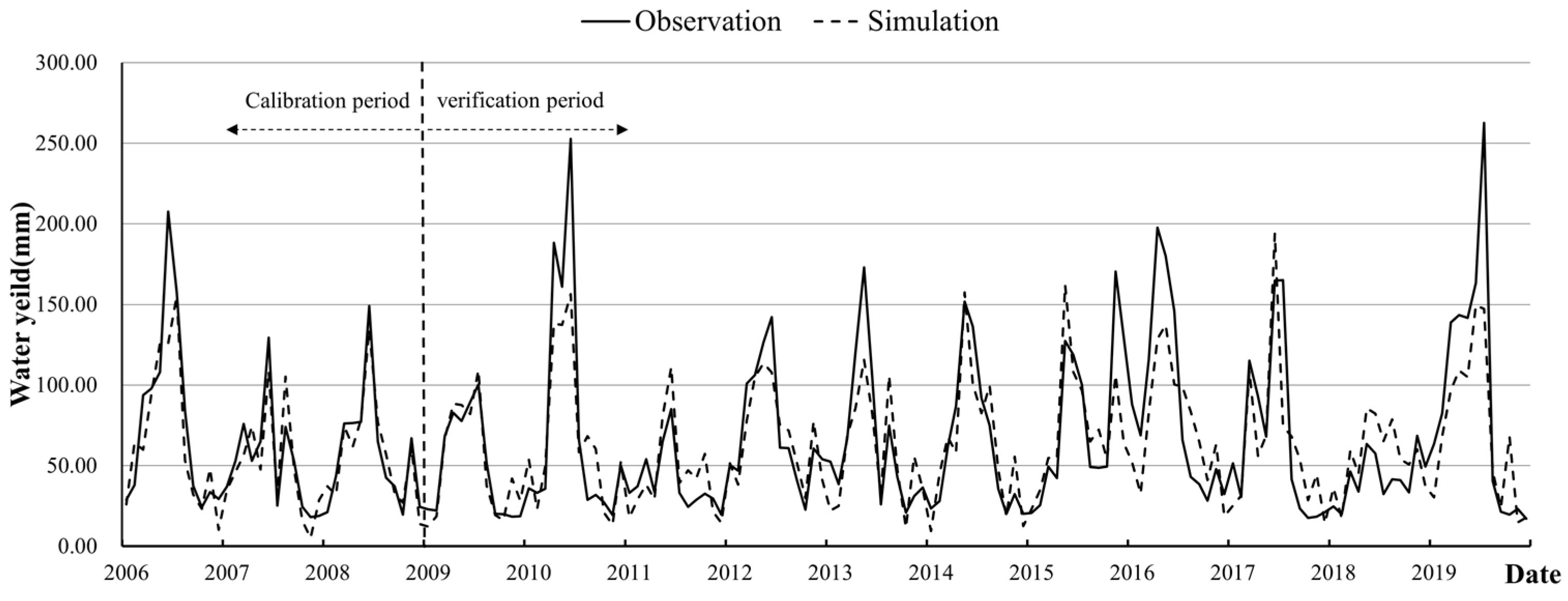
3.1.2. Parameter Validation

The evaluation of the simulation effect of water yield is shown in

Table 7. Evaluation of the Simulation Effect of Water yield in the XRB.

Study Period	NSE	R2
Calibration period	0.80	0.81
Verification period	0.71	0.72

; the calibration period NSE = 0.80, R² = 0.81, and the verification period NSE = 0.71, R² = 0.72. The seasonal water-yield InVEST model for the XRB established in this study has a good simulation effect and can be further studied.

3.2. Spatiotemporal Evolution of Water Yield

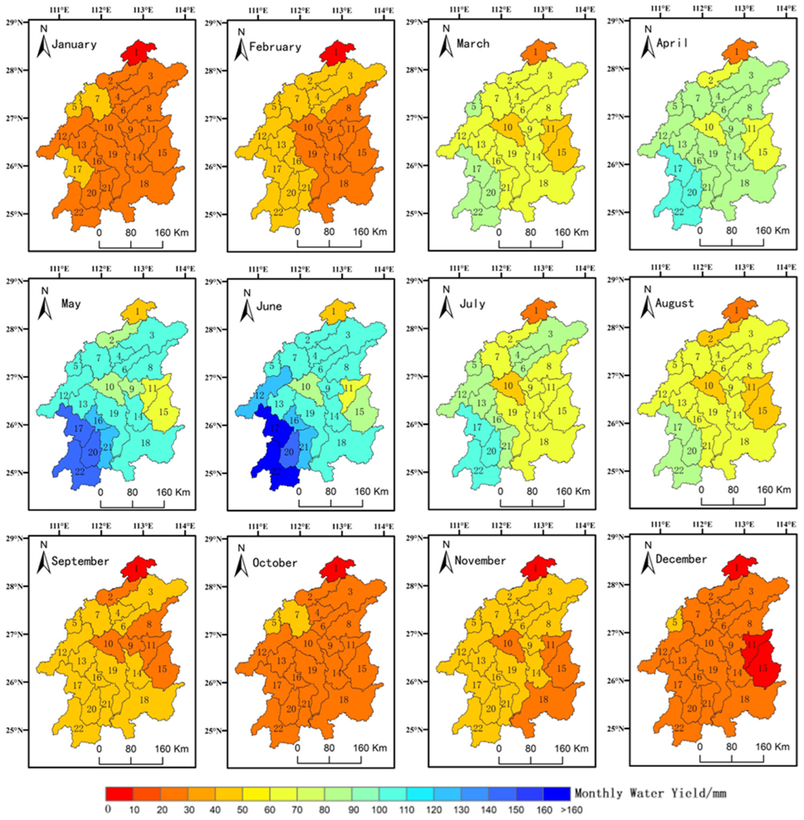
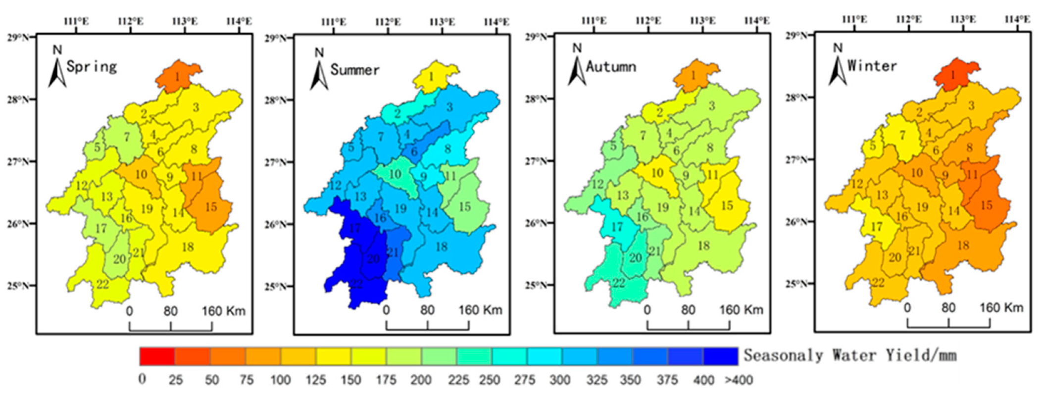
3.2.1. Spatiotemporal Evolution Characteristics

We selected 2006–2009 as the calibration period and 2010–2020 as the validation period. Figure 4 shows the simulated water-yield results for the XRB. The simulated results and the actual data showed a high degree of fit.

The spatial variation characteristics of the multi-year monthly average water yield and the spatial variation characteristics of the multi-year quarterly average water yield are shown in Figure 5 and Figure 6, in which the monthly and quarterly water yields are the average values for the study period (2006–2020). On the monthly scale, the characteristics of the average monthly water yields for many years are as follows: the water yield from January to June presents a gradual upward trend, while there is a shift to a downward trend from June to October, which rises again slightly from October to November and then converts to a decreasing trend from November to December. On the seasonal scale, the annual average seasonal water yield is characterized by a gradual increase from spring to summer and a gradual decrease from summer to winter. In general, the spatial variation in water production showed an increasing trend from northeast to southwest. The northern watershed 1, the central watershed 10, and the eastern watersheds 11 and 15 are areas with low water yields, and the southwestern watersheds 17, 20 and 22 are areas with high water yields.

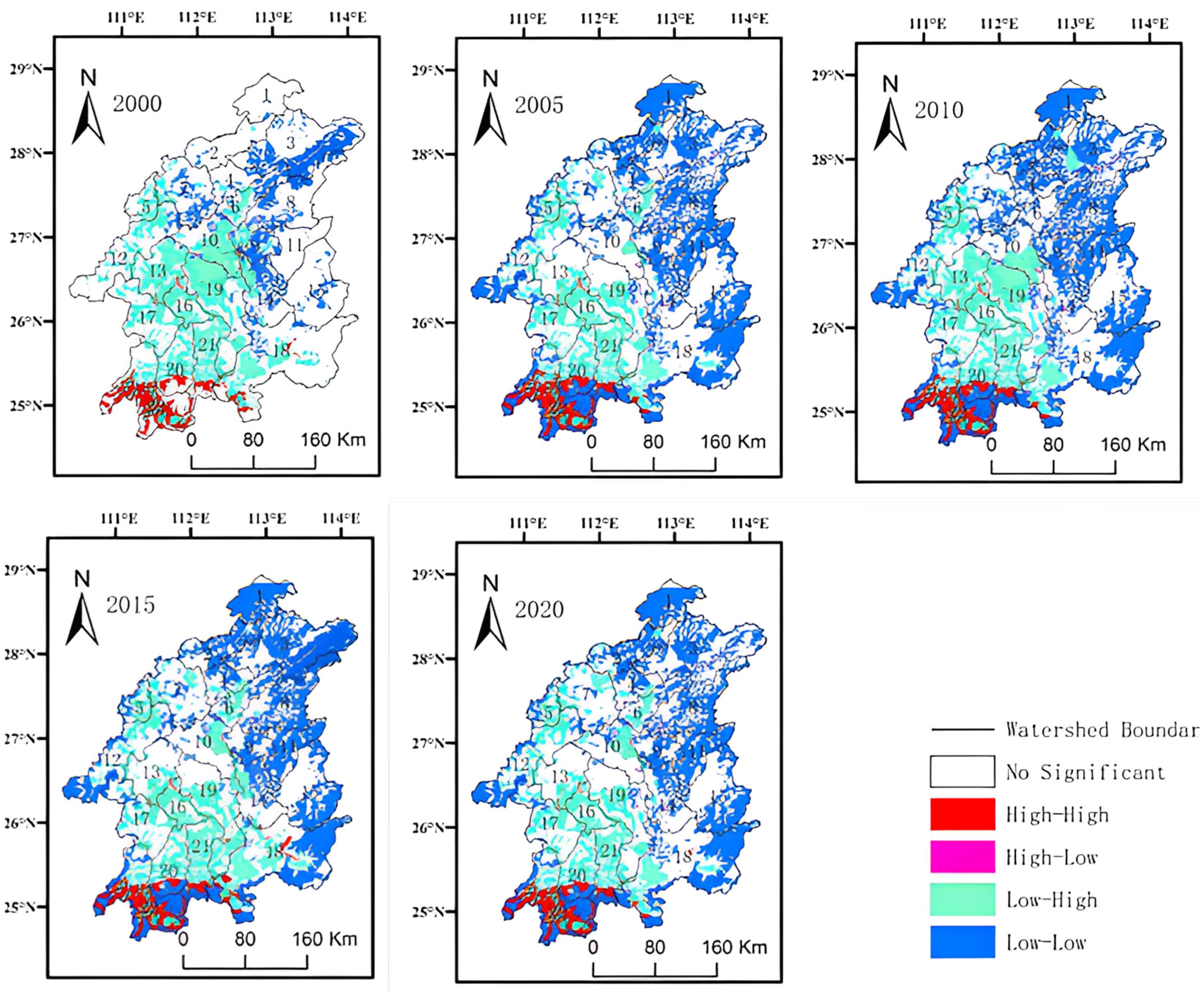
3.2.2. Spatial Autocorrelation Analysis

It can be seen from Figure 7 that, from 2006 to 2020, the XRB was dominated by low–high aggregation sub-basins and low–low aggregation sub-basins. The low–high aggregation sub-basins were mainly distributed in the central, western and southern areas, including watersheds 5, 6, 10, 12, 13, 16, 17, 18, 14, 19, 20 and 21, while the low–low aggregation sub-basins were the most widely distributed, including watersheds 1, 2, 3, 4, 7, 8, 11, 14, 15, 18, 12 and 22. The high–high aggregation sub-basins were less widely distributed and were concentrated in basin 22 in the southern area of the XRB. In general, from 2006 to 2020, basins 1, 2 and 3 in the north and basins 8, 9, 11, 15 and 18 in the east were the main distribution areas of the low–low aggregation sub-basins, that is, the areas with low water-yield values. Basin 22 in the south of the XRB was the main distribution area of the high–high aggregation sub-basin, that is, the high-value area.

3.3. Impact of Climate Change and Land-Use Change on Water Yield

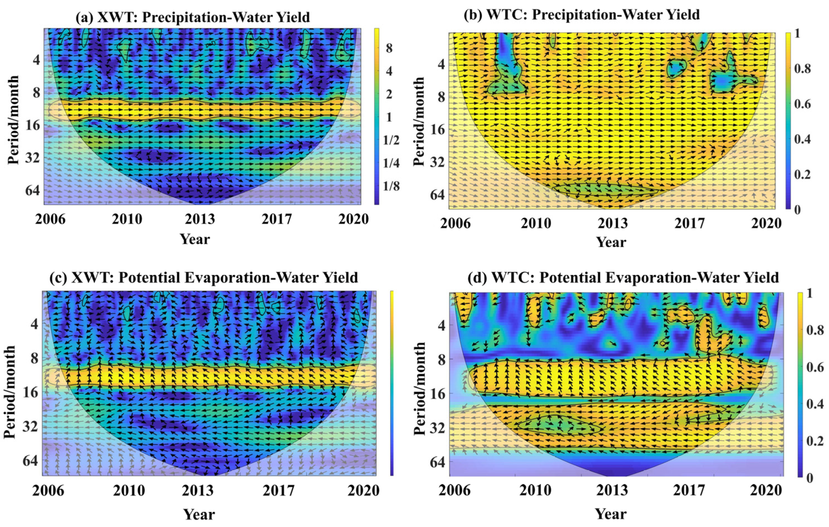
3.3.1. Impact of Climate Change on Water Yield

Figure 8 shows the cross-wavelet results for monthly rainfall, potential evapotranspiration and water yield. There was a resonance period of 10–15 months between rainfall and water yield from 2006 to 2019. The phase difference arrows of the two were horizontal to the right, indicating that they were positively correlated. Potential evapotranspiration and water yield also had a resonance period of 10–15 months from 2006 to 2019, and the phase difference arrow between the two also reflected that the change in potential evapotranspiration was 3 to 4.5 months earlier than that for water yield. In the low-energy region, potential evapotranspiration and water yield had 8–16- and 18–48-month cycles between 2004 and 2016, in addition to intermittent oscillations of 1–8 months, with the phase difference arrow horizontal to the left, indicating that they were negatively correlated.

As shown in

Table 8. The correlation analysis and statistics for water yield, precipitation and potential evapotranspiration.

Climate Factor	R	R2	Sig.
Precipitation Potential evapotranspiration	0.994 −0.454	0.987 0.206	0.0001 0.0001

, SPSS was used to perform a correlation analysis of rainfall, potential evapotranspiration and water yield. In terms of correlation, water yield was significantly positively correlated with rainfall, with a correlation coefficient of 0.994; however, it was negatively correlated with potential evapotranspiration, with a correlation coefficient of −0.454. This can also prove that rainfall is the decisive factor affecting water yield and that potential evapotranspiration is an important factor.

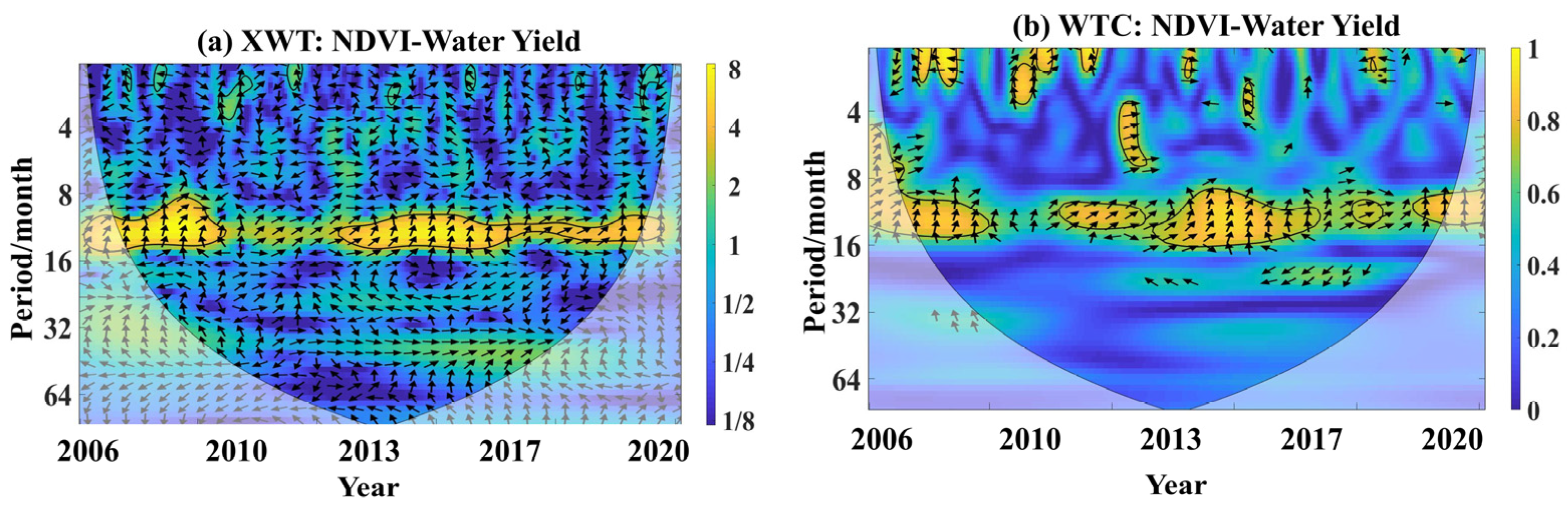
3.3.2. Impact of Land-Use Change on Water Yield

As shown in

Table 9. Correlation analysis results for land use and water yield.

Land Use	R	R2	Sig.
Farmland	−0.138	0.028	0.236
Woodland	−0.132	0.015	0.296
Grassland	−0.078	0.006	0.369
Water	0.078	0.006	0.369
Construction land	0.166	0.019	0.275
Unused land	−0.128	0.016	0.290

, the correlations between each of the land-use types and water yield were analyzed using SPSS. From a correlational point of view, a slight negative correlation was found to exist between water yield and farmland, and the correlation coefficient was −0.138. Water yield was both weakly and negatively correlated with woodland and grassland, with correlation coefficients of −0.132 and −0.078, respectively. On the contrary, water yield was both weakly and positively correlated with water and construction land, with correlation coefficients of 0.078 and 0.166, respectively. Finally, water yield was weakly and negatively correlated with unused land, and the correlation coefficient was −0.128. Therefore, according to the correlations, the order of the impacts of each of the land-use types on water yield was: construction land > farmland > woodland > unused land > water = grassland.

Figure 9 shows the cross-wavelet results for monthly normalized vegetation index (NDVI) and water yield. During 2006 to 2009, there was a resonance period of 8–14 months between NDVI and water yield, and during 2012 to 2018, there was a resonance period of 12–15 months. The phase difference arrow direction in the figure indicates that the change in NDVI was 3 months ahead of the change in water yield. In the low-energy region, NDVI and water yield showed intermittent fluctuations of 8–16 months and small-scale intermittent fluctuations of 1–4 months. The arrow direction of phase difference between the two shows that the change in NDVI occurred 3 months earlier than the change in water yield and that they were positively correlated.

3.3.3. Attribution Quantitative Identification

The attribution analysis results for 2006 to 2020 are shown in

Table 10. Attribution Analysis of Water yield in the XRB.

Change Factors	Contribution/mm	Contribution Rate/%
Climate change	64.86	67.08
Land use	−31.83	32.92

; climate change was found to be the dominant factor causing water-yield changes [38,39,40], its contribution rate being as high as 67.08%, causing an increase in water yield of 64.86 mm. The impacts of land-use changes were less than those of climate change, whose contribution rate was only 32.92%, leading to a reduction of 31.83 mm in water yield.

4. Discussion

4.1. Comparison with Others

The water-yield spatial distribution pattern in the XRB was generally consistent with that for precipitation, but there was a special situation that appeared in the central region, namely, relatively low average water yield with relatively high average precipitation. The impact of terrain factors on water yield needs to be considered [41,42]. During the period of 2010 to 2020, the spatial aggregation benefits of water yield were more obvious in the southwest of the XRB than in the previous decade. The water-yield aggregation area is the key area of human activities, which confirms that the policy and economic drive led to the expansion of construction land, and changes in the spatial pattern of land caused by human activities will have impacts on water yield [43]. Therefore, towns should promote the planning and construction of green spaces to reduce the impact of urban heat islands and prevent flood risks. Farmland and grassland should be rationally laid out, and agricultural development on steep slopes should be strictly controlled. Improved water conservancy facilities and enhanced agricultural water resources are needed to implement the green recycling utilization of ecological water resources [44]. From 2006 to 2009, the XRB underwent a process of rapid urbanization, with a substantial increase in construction land and industrial and mining land. Although such expansion would lead to water yield increasing, it was difficult for precipitation to be recycled after reaching the artificial surface, which resulted in adverse effects, such as reduced groundwater recharge and increased flood risk. Therefore, in the planning process, the hydrological and ecological effects caused by land-use changes should be considered and the scale and speed of development of towns should be controlled. Moreover, ecological development should also be considered [45,46]. Through this study, it was found that climate change is the main factor affecting water-yield change in the XRB, while land use has less of an effect. This result is consistent with relevant research conclusions on the impacts of water yield in the Weihe River Basin [47] and Miyaluo Forest Farm [48], and the quantitative attribution analysis results are consistent with relevant research conclusions regarding the Shule River Basin [14] and the Southwest Karst Basin [49]. Climate change will significantly affect water yield in the long term, while land use will also have a certain impact on water yield in the short term [18]. Land-use changes, in turn, will affect local climate and thus affect water-yield changes [50]. For example, forests can affect climate through water recycling and the redistribution of precipitation, and urbanization leads to urban heat-island effects that cause significant changes to local climates. Therefore, the mechanism governing how land use impacts the water-yield functions of ecosystems still needs to be further studied.

Although the water-yield results in this study are consistent with the results of the study of Yang Dong [51], the study in this paper is based on the existing climate and land-use conditions. We should carry out predictive research on water yield, combining climate-change prediction and land-use prediction based on the Global Climate Model (GCM) and the PLUS model in the future. This research focuses on describing the natural water cycle, while water yield is also greatly affected by human activities, mainly reflected in land-use change in this paper. In the future, studies on the impacts of human activities, such as water conservancy projects, soil- and water-conservation measures, and artificial water withdrawal, on water yield in the basin should be carried out.

4.2. Contribution Rate Based on the Budyko Assumption

Based on the annual data for the XRB from 2006 to 2009, during the study period, the average annual water yield (R) = 843.83 mm, the annual average rainfall (P) = 1457.96 mm and the annual average potential evapotranspiration (E₀) = 2132.63 mm. The value of the characteristic parameter w of the underlying surface of the XRB in the base period could be obtained by least squares analysis, and it was 1.390. The values for water yield and meteorological changes in the characteristic parameters of the underlying surface of the watershed are shown in

Table 11. Changes in water yield, meteorology and characteristic parameters of the underlying surface of the basin during the base period and the change period.

Research Period	R/mm	P/mm	E/mm	$\mathit{w}$
Calibration period	843.83	1457.96	2132.63	1.390
Verification period	862.22	1504.94	2076.75	1.414

[52].

The contribution amounts and contribution rates of rainfall change, evapotranspiration change and underlying surface change to water-yield change were calculated at the annual scale, as shown in

Table 12. Attribution Analysis of the Contribution Rate Model.

Changing Factors	Contribution/mm	Contribution Rate/%
Land use	−24.34	36.29
Climate change	42.73	63.71
Evapotranspiration	7.15	10.66
Precipitation	35.58	53.05

. From Table 12, it can be seen that the contribution rate of rainfall change was the highest, indicating that change in rainfall had the greatest impact on water yield. Change in land use (underlying surface) followed. The contribution rate for evapotranspiration change was the lowest. If precipitation and evapotranspiration are classified as climate change, the contribution rate of climate change to water-yield change was 63.71% and that of land-use change was 36.29%.

Comparing the water-yield simulation results of the InVEST seasonal water-yield model and those obtained according to the Budyko assumption, the former are better [53]. The contribution rate of climate change obtained with the InVEST seasonal water-yield model was higher than that obtained according to the Budyko assumption, while the contribution rate of land use was lower.

5. Conclusions

With the acceleration of urbanization, the ecosystem of the XRB has undergone significant changes. Clarifying the temporal and spatial water-yield evolution characteristics in the XRB and identifying the influencing factors play a vital role in the sustainable development of the XRB. That is the reason why we studied these two aspects in this study. The results are expected to provide scientific assistance and a reference that will be beneficial for optimizing the allocation of water resources and protecting and rationally developing water resources in the basin to achieve the sustainable development of the ecosystem. The main conclusions of this study are as follows:

(1) Temporal and spatial evolution of water yield in the XRB. The average monthly water yield in the XRB over the years is as follows: it gradually increases from January to June, gradually decreases from June to October, slightly increases from October to November and tends to decrease from November to December. The multi-year seasonal average water yield is characterized by a gradual increase from spring to summer and a gradual decrease from summer to winter. The spatial variation in water yield in the XRB showed an increasing trend from north to south and from east to west. The spatial autocorrelation analysis method was used to analyze water yield in the XRB. The results showed that Basin Nos. 1, 2 and 3 in the north of the XRB and Basin Nos. 8, 9, 11, 15 and 18 in the east of the XRB had low water yields and that Basin No. 22 in the south had a high water yield.

(2) Analysis of the influence of climate-change factors on water production. According to the cross-wavelet analysis results for rainfall, potential evapotranspiration and water yield and rainfall and water yield are positively correlated, while potential evapotranspiration and water yield are negatively correlated, and the change in potential evapotranspiration does not cause a change in water yield until 3 to 4.5 months after the change in potential evapotranspiration.

(3) Analysis of the influence of land-use-change factors on water yield. From 2006 to 2020, the decreases in unused land, grassland, woodland and farmland as well as the increases in water and construction land all had a positive impact on the increase in farmland water yield in the XRB. Among these changes, the change in construction land had the greatest influence on the increase in water yield. According to the cross-wavelet analysis results for NDVI and water yield, there was a positive correlation between NDVI and water yield, and the change in water yield was not caused until 3 months after the change in NDVI.

(4) Attribution analysis of water-yield evolution. Compared with the InVEST model, the simulation accuracy of the seasonal water-yield module based on the Budyko hypothesis was lower, but the attribution results were similar. Climate change was the main factor that caused the change in water yield in the XRB from 2006 to 2020, with the contribution rate ranging from 63.71%~67.08%. Land-use change was a secondary factor in water-yield change in the XRB, and the contribution rate was 32.92%~36.29%.

References

1. Lang, Y.Q.; Song, W.; Zhang, Y. Responses of the water-yield ecosystem service to climate and land use change in Sancha River Basin, China. Phys. Chem. Earth 2017, 101, 102–111. [Google Scholar] [CrossRef]
2. Wang, J.H.; Shang, Y.Z.; Wang, H.; Zhao, Y.; Yin, Y. Beijing’s Water Resources: Challenges and Solutions. J. Am. Water Resour. Assoc. 2015, 51, 614–623. [Google Scholar] [CrossRef]
3. Deng, X.Z.; Zhao, C.H. Identification of Water Scarcity and Providing Solutions for Adapting to Climate Changes in the Heihe River Basin of China. Adv. Meteorol. 2015, 2015, 279173. [Google Scholar] [CrossRef] [Green Version]
4. Shomar, B.; Dare, A. Ten key research issues for integrated and sustainable wastewater reuse in the Middle East. Environ. Sci. Pollut. Res. 2015, 22, 5699–5710. [Google Scholar] [CrossRef]
5. Ako, A.A.; Eyong, G.E.T.; Nkeng, G.E. Water Resources Management and Integrated Water Resources Management (IWRM) in Cameroon. Water Resour. Manag. 2010, 24, 871–888. [Google Scholar] [CrossRef]
6. Lu, H.T.; Yan, Y.; Zhu, J.Y.; Jin, T.T.; Liu, G.H.; Wu, G.; Stringer, L.C.; Dallimer, M. Spatiotemporal Water Yield Variations and Influencing Factors in the Lhasa River Basin, Tibetan Plateau. Water 2020, 12, 1498. [Google Scholar] [CrossRef]
7. Li, G.Y.; Jiang, C.H.; Zhang, Y.H.; Jiang, G.H. Whether land greening in different geomorphic units are beneficial to water yield in the Yellow River Basin? Ecol. Indic. 2021, 120, 106926. [Google Scholar] [CrossRef]
8. Niu, P.T.; Zhang, E.C.; Feng, Y.; Peng, P.H. Spatial-Temporal Pattern Analysis of Land Use and Water Yield in Water Source Region of Middle Route of South-to-North Water Transfer Project Based on Google Earth Engine. Water 2022, 14, 2535. [Google Scholar] [CrossRef]
9. Polasky, S.; Nelson, E.; Pennington, D.; Johnson, K.A. The Impact of Land-Use Change on Ecosystem Services, Biodiversity and Returns to Landowners: A Case Study in the State of Minnesota. Environ. Resour. Econ. 2011, 48, 219–242. [Google Scholar] [CrossRef]
10. Leh, M.D.K.; Matlock, M.D.; Cummings, E.C.; Nalley, L.L. Quantifying and mapping multiple ecosystem services change in West Africa. Agric. Ecosyst. Environ. 2013, 165, 6–18, Erratum in Agric. Ecosyst. Environ. 2016, 221, 285. [Google Scholar] [CrossRef]
11. Marques, M.; Bangash, R.F.; Kumar, V.; Sharp, R.; Schuhmacher, M. The impact of climate change on water provision under a low flow regime: A case study of the ecosystems services in the Francoli river basin. J. Hazard. Mater. 2013, 263, 224–232. [Google Scholar] [CrossRef] [PubMed]
12. Gao, J.; Li, F.; Gao, H.; Zhou, C.B.; Zhang, X.L. The impact of land-use change on water-related ecosystem services: A study of the Guishui River Basin, Beijing, China. J. Clean Prod. 2017, 163, S148–S155. [Google Scholar] [CrossRef]
13. Wang, J.X.; Huang, J.K.; Yan, T.T. Impacts of Climate Change on Water and Agricultural Production in Ten Large River Basins in China. J. Integr. Agric. 2013, 12, 1267–1278. [Google Scholar] [CrossRef]
14. Wei, P.J.; Chen, S.Y.; Wu, M.H.; Deng, Y.F.; Xu, H.J.; Jia, Y.L.; Liu, F. Using the InVEST Model to Assess the Impacts of Climate and Land Use Changes on Water Yield in the Upstream Regions of the Shule River Basin. Water 2021, 13, 1250. [Google Scholar] [CrossRef]
15. Yin, G.D.; Wang, X.; Zhang, X.; Fu, Y.S.; Hao, F.H.; Hu, Q.H. InVEST Model-Based Estimation of Water Yield in North China and Its Sensitivities to Climate Variables. Water 2020, 12, 1692. [Google Scholar] [CrossRef]
16. Villamizar, S.R.; Pineda, S.M.; Carrillo, G.A. The Effects of Land Use and Climate Change on the Water Yield of a Watershed in Colombia. Water 2019, 11, 285. [Google Scholar] [CrossRef] [Green Version]
17. Hu, T.; Wu, J.S.; Li, W.F. Assessing relationships of ecosystem services on multi-scale: A case study of soil erosion control and water yield in the Pearl River Delta. Ecol. Indic. 2019, 99, 193–202. [Google Scholar] [CrossRef]
18. Zhang, X.; Zhang, G.S.; Long, X.; Zhang, Q.; Liu, D.S.; Wu, H.J.; Li, S. Identifying the drivers of water yield ecosystem service: A case study in the Yangtze River Basin, China. Ecol. Indic. 2021, 132, 108304. [Google Scholar] [CrossRef]
19. Goshime, D.W.; Haile, A.T.; Absi, R.; Ledésert, B. Impact of water resource development plan on water abstraction and water balance of Lake Ziway, Ethiopia. Sustain. Water Resour. Manag. 2021, 7, 36. [Google Scholar] [CrossRef]
20. Wang, G.; Zhang, J.; Xu, Y.; Bao, Z.; Yang, X. Estimation of future water resources of Xiangjiang River Basin with VIC model under multiple climate scenarios. Water Sci. Eng. 2017, 10, 87–96. [Google Scholar] [CrossRef]
21. Xu, X.; Sheng, D.; Li, G.; Chen, X.; Wang, X.; Xiao, C.; Gao, X.; Hu, C. Comprehensive Assessment of the Water Ecological Security of the Xiangjiang River Basin Based on Physico-Chemistry and Organism Indices. Appl. Ecol. Environ. Res. 2019, 17, 4547–4574. [Google Scholar] [CrossRef]
22. Rey, J.M. Modelling potential evapotranspiration of potential vegetation. Ecol. Model. 1999, 123, 141–159. [Google Scholar] [CrossRef]
23. Fu, B.; Xu, P.; Wang, Y.; Peng, Y.; Ren, J. Spatial Pattern of Water Retetnion in Dujiangyan County. Acta Ecol. Sin. 2013, 33, 789–797. [Google Scholar] [CrossRef]
24. Khzr, B.O.; Ibrahim, G.R.F.; Hamid, A.A.; Ail, S.A. Runoff estimation using SCS-CN and GIS techniques in the Sulaymaniyah sub-basin of the Kurdistan region of Iraq. Environ. Dev. Sustain. 2022, 24, 2640–2655. [Google Scholar] [CrossRef]
25. Auerswald, K.; Gu, Q.L. Reassessment of the hydrologic soil group for runoff modelling. Soil Tillage Res. 2021, 212, 105034. [Google Scholar] [CrossRef]
26. Stewart, D.; Canfield, E.; Hawkins, R. Curve Number Determination Methods and Uncertainty in Hydrologic Soil Groups from Semiarid Watershed Data. J. Hydrol. Eng. 2012, 17, 1180–1187. [Google Scholar] [CrossRef]
27. Feng, K.X.; Lu, Z.Z.; Yang, C.Q. Enhanced Morris method for global sensitivity analysis: Good proxy of Sobol’ index. Struct. Multidiscip. Optim. 2019, 59, 373–387. [Google Scholar] [CrossRef]
28. Gao, Y.; Sha, X.; Xiangyang, X.U.; Yin, Y.; Peng, L.I. Sensitivity analysis of SWMM model parameters based on Morris method. J. Water Resour. Water Eng. 2016, 27, 87–90. [Google Scholar] [CrossRef]
29. Huo, A.D.; Huang, Z.K.; Cheng, Y.X.; Van Liew, M.W. Comparison of two different approaches for sensitivity analysis in Heihe River basin (China). Water Supply 2020, 20, 319–327. [Google Scholar] [CrossRef]
30. Torrence, C.; Compo, G.P. A practical guide to wavelet analysis. Bull. Amer. Meteorol. Soc. 1998, 79, 61–78. [Google Scholar] [CrossRef]
31. Grinsted, A.; Moore, J.C.; Jevrejeva, S. Application of the cross wavelet transform and wavelet coherence to geophysical time series. Nonlinear Process. Geophys. 2004, 11, 561–566. [Google Scholar] [CrossRef]
32. Gui, Y.P.; Wang, Q.M.; Zhao, Y.; Dong, Y.Y.; Li, H.H.; Jiang, S.; He, X.; Liu, K. Attribution analyses of reference evapotranspiration changes in China incorporating surface resistance change response to elevated CO2. J. Hydrol. 2021, 599, 126387. [Google Scholar] [CrossRef]
33. Sun, X.Y.; Wang, Y.D. Attribution Analysis of Annual Precipitation Simulation Differences and Its Correction of CMIP5 Climate Models on the Chinese Mainland. Atmosphere 2022, 13, 382. [Google Scholar] [CrossRef]
34. Tabari, H.; Asr, N.M.; Willems, P. Developing a framework for attribution analysis of urban pluvial flooding to human-induced climate impacts. J. Hydrol. 2021, 598, 126352. [Google Scholar] [CrossRef]
35. Lian, X.H.; Qi, Y.; Wang, H.W.; Zhang, J.L.; Yang, R. Assessing Changes of Water Yield in Qinghai Lake Watershed of China. Water 2020, 12, 11. [Google Scholar] [CrossRef] [Green Version]
36. Guo, A.J.; Chang, J.X.; Wang, Y.M.; Huang, Q.; Guo, Z.H.; Li, Y.Y. Uncertainty analysis of water availability assessment through the Budyko framework. J. Hydrol. 2019, 576, 396–407. [Google Scholar] [CrossRef]
37. Gan, G.J.; Liu, Y.B.; Sun, G. Understanding interactions among climate, water, and vegetation with the Budyko framework. Earth-Sci. Rev. 2021, 212, 103451. [Google Scholar] [CrossRef]
38. Gou, J.J.; Miao, C.Y.; Duan, Q.Y.; Tang, Q.H.; Di, Z.H.; Liao, W.H.; Wu, J.W.; Zhou, R. Sensitivity Analysis-Based Automatic Parameter Calibration of the VIC Model for Streamflow Simulations Over China. Water Resour. Res. 2020, 56, e2019WR025968. [Google Scholar] [CrossRef] [Green Version]
39. Sun, L.; Li, Z.J.; Zhang, K.; Jiang, T.T. Impacts of precipitation and topographic conditions on the model simulation in the north of China. Water Supply 2021, 21, 1025–1035. [Google Scholar] [CrossRef]
40. Chen, X.Y.; Quan, Q.; Zhang, K.; Wei, J.H. Spatiotemporal characteristics and attribution of dry/wet conditions in the Weihe River Basin within a typical monsoon transition zone of East Asia over the recent 547 years. Environ. Modell. Softw. 2021, 143, 105116. [Google Scholar] [CrossRef]
41. Liu, N.; Sun, P.S.; Caldwell, P.V.; Harper, R.; Liu, S.R.; Sun, G. Trade-off between watershed water yield and ecosystem productivity along elevation gradients on a complex terrain in southwestern China. J. Hydrol. 2020, 590, 125449. [Google Scholar] [CrossRef]
42. Ma, S.; Li, Y.; Zhang, Y.H.; Wang, L.J.; Jiang, J.; Zhang, J.C. Distinguishing the relative contributions of climate and land use/cover changes to ecosystem services from a geospatial perspective. Ecol. Indic. 2022, 136, 108645. [Google Scholar] [CrossRef]
43. Rohatyn, S.; Rotenberg, E.; Ramati, E.; Tatarinov, F.; Tas, E.; Yakir, D. Differential Impacts of Land Use and Precipitation on “Ecosystem Water Yield”. Water Resour. Res. 2018, 54, 5457–5470. [Google Scholar] [CrossRef]
44. Li, J.H.; Zhou, K.C.; Xie, B.G.; Xiao, J.Y. Impact of landscape pattern change on water-related ecosystem services: Comprehensive analysis based on heterogeneity perspective. Ecol. Indic. 2021, 133, 108372. [Google Scholar] [CrossRef]
45. Han, Z.L.; Cui, S.X.; Yan, X.L.; Liu, C.H.; Li, X.Y.; Zhong, J.Q.; Wang, X.Z. Guiding sustainable urban development via a multi-level ecological framework integrating natural and social indicators. Ecol. Indic. 2022, 141, 109142. [Google Scholar] [CrossRef]
46. Liu, J.; Li, J.; Qin, K.; Zhou, Z.; Yang, X.; Li, T. Changes in land-uses and ecosystem services under multi-scenarios simulation. Sci. Total Environ. 2017, 586, 522–526. [Google Scholar] [CrossRef]
47. Wu, C.X.; Qiu, D.X.; Gao, P.; Mu, X.M.; Zhao, G.J. Application of the InVEST model for assessing water yield and its response to precipitation and land use in the Weihe River Basin, China. J. Arid. Land 2022, 14, 426–440. [Google Scholar] [CrossRef]
48. Zhang, Y.D.; Liu, S.R.; Wei, X.H.; Liu, J.T.; Zhang, G.B. Potential Impact of Afforestation on Water Yield in the Subalpine Region of Southwestern China. J. Am. Water Resour. Assoc. 2008, 44, 1144–1153. [Google Scholar] [CrossRef]
49. Wu, L.H.; Wang, S.J.; Bai, X.Y.; Luo, W.J.; Tian, Y.C.; Zeng, C.; Luo, G.J.; He, S.Y. Quantitative assessment of the impacts of climate change and human activities on runoff change in a typical karst watershed, SW China. Sci. Total Environ. 2017, 601, 1449–1465. [Google Scholar] [CrossRef]
50. Ghimire, U.; Shrestha, S.; Neupane, S.; Mohanasundaram, S.; Lorphensri, O. Climate and land-use change impacts on spatiotemporal variations in groundwater recharge: A case study of the Bangkok Area, Thailand. Sci. Total Environ. 2021, 792, 148370. [Google Scholar] [CrossRef]
51. Yang, D.; Liu, W.; Tang, L.Y.; Chen, L.; Li, X.Z.; Xu, X.L. Estimation of water provision service for monsoon catchments of South China: Applicability of the InVEST model. Landsc. Urban Plan. 2019, 182, 133–143. [Google Scholar] [CrossRef]
52. Yang, H.; Xu, H.; Huntingford, C.; Ciais, P.; Piao, S. Strong direct and indirect influences of climate change on water yield confirmed by the Budyko framework. Geogr. Sustain. 2021, 2, 281–287. [Google Scholar] [CrossRef]
53. Li, H.J.; Shi, C.X.; Zhang, Y.S.; Ning, T.T.; Sun, P.C.; Liu, X.F.; Ma, X.Q.; Liu, W.; Collins, A.L. Using the Budyko hypothesis for detecting and attributing changes in runoff to climate and vegetation change in the soft sandstone area of the middle Yellow River basin, China. Sci. Total Environ. 2020, 703, 135588. [Google Scholar] [CrossRef] [PubMed]
Figure 1. Geographical location of the study area and distribution map of meteorological stations.
Water 15 00514 g001
Figure 2. (a) Rainfall for January 2006. (b) Potential evapotranspiration for January 2006. (c) Sub-watershed. (d) Land-use map of the XRB in 2006. (e) Grouping charts for hydrological soils.
Water 15 00514 g002
Figure 3. Model parameter sensitivity analysis results.
Water 15 00514 g003
Figure 4. Simulation results for monthly water yield in the XRB (2006–2020).
Water 15 00514 g004
Figure 5. Spatial variation in monthly average water yield.
Water 15 00514 g005
Figure 6. Spatial variation in seasonal average water yield.
Water 15 00514 g006
Figure 7. LISA cluster map of water yields in the XRB from 2006 to 2020.
Water 15 00514 g007
Figure 8. Cross-Wavelet Results for Precipitation, Potential Evapotranspiration and Water Yield in the XRB.
Water 15 00514 g008
Figure 9. Cross-wavelet results for NDVI and water yield.
Water 15 00514 g009