Statistical Methods and Models for Pollutant Control in Municipal Surface Waters

Abstract

This paper aims to systematize a series of statistical methods of analysis and control and proposes some forecast models for surface water pollution both in and near a large city. The monitoring data of heavy metals, nitrites, and phosphates collected for three years are processed using different statistical tools. It is demonstrated that they are under statistical control, and appropriate mathematical models are formulated to allow for forecasting and understanding of the causes of the appearance and perpetuation of certain phenomena. A comparative analysis is made, and the generalization of some methods is considered as an analysis and control tool.

1. Introduction

Statistical tools are considered important elements in water quality analysis. Multivariate statistical techniques (MSTs) represent a very interesting approach as many works prove, followed by concrete case studies like in Wang et al. [1], where discriminant analysis, principal component analysis, and factor analysis have been involved. Among the multivariate statistical methods, factor analysis and cluster analysis are applied by Ismail et al. [2] to identify the principal factors and pollution sources that affect the water quality of the Danube River and to evaluate the spatial and temporal similarities or dissimilarities among the sites for sampling and monitoring periods. The quality of water can be evaluated by analyzing its physical, chemical, and biological characteristics. The use of cluster analysis, multivariate statistical methods, principal component analysis, and factor analysis for the interpretation and analysis of water quality data have been presented in [3]. To identify the sources of pollution and to obtain a better understanding of changes in the quality of surface water, these statistical techniques are useful. The use of multivariate statistical methods in the monitoring data gives information about the chemical structure of water bodies. Also, in Hue et al. [4], the assessment of spatial variability and the determination of the main contamination in surface water quality using multivariate statistical analysis techniques, considering principal component analysis and cluster analysis, has been performed.

Water management, involving monitoring techniques that accurately assess the water quality and determine the effects of pollution using multivariate statistical methods and water quality, is proposed to evaluate the processes controlling water chemical composition and the overall water quality status in da Silva et al. [5], where a holistic approach for the water quality conditions and related effects has been performed. Once again, the multivariate statistical techniques to assess the quality of surface waters are used by Dawood et al. [6] by studying the temporal and spatial water quality variability to reveal the characteristics and pollution indicators. Water evaluation via multivariate statistical techniques was also proposed in [7,8,9,10,11,12] followed by study cases that, actually, justify the statistical approaches, and it is sustained using these mathematical approaches.

Multivariate statistical techniques combined with water quality identification index represent one of the most useful combinations that realize accurate monitoring and the assessment of water quality, i.e., the spatiotemporal analysis of water quality, as in works by [13,14,15] for surface water quality and also for groundwater in the case of [15]. MSTs have also been successfully applied to solve similar issues in [16,17,18].

However, not only MSTs represent the statistical studies for waters, especially surface waters. Many other statistical methods and models can be remarkably cited in this kind of analysis, as in the papers of Mohammed et al. [19], Bărbulescu et al. [20], Schreiber et al. [21], Kovrov et al. [22], Antonopoulos et al. [23], Majerek et al. [24], Stričević et al. [25], Khouri et al. [26], Bhat et al. [27], and Le et al. [28].

Statistical tools in the analysis of water quality to process the collected data have been used and capitalized in papers, as that of Andrejiová et al. [29] and Wang et al. [30], book chapters by Fu et al. [31], and more extended works, as that of Helsel and Hirsch [32], Bal [33], and Hajigholizadeh [34].

The author of this work used statistical methods in environmental monitoring, especially for atmospheric evaluation in [35,36,37,38,39,40,41] and control of water pollutants, in [42,43,44]. As specific methods applied in cited works, we can highlight the demonstrations that the analyzed data are under statistical control and use the most involved model of time series, with a lot of important properties of this powerful instrument. Statistical control can be used for monitoring the degree of water pollution in a considered zone. The aim of the usage of the time series properties is to understand the driving forces and internal structures that produce the observed data, to organize the data into a model, and to involve them in forecasting, monitoring, or even feedback and feedforward control. The most important difference between modeling data via time series methods and using the process monitoring methods is that, in time series analysis, the data collected over time may present internal structure such as autocorrelation, trend, or seasonal variation.

In this paper, data, methods, and models from previous papers [42,43,44] are analyzed and discussed in order to deepen and systematize appropriate instruments and procedures to control the pollution of surface waters in or near a big town. The data collected for certain pollutants in two periods of time and analyzed in the above three cited papers, together with the statistical methods used there, have been discussed and compared in order to highlight mathematical models that can govern such phenomena, to capitalize on some statistical instruments that can be used to control such processes. Also, the approach in this study is able to be replicated, so it can be adapted accordingly in similar situations, other data representing a new study, and, therefore, the methods and models used here can be in a certain way generalized and exemplified.

2. Materials and Methods Analysis

The monitored pollutants for surface waters in and near Bucharest are heavy metals such as lead, monitored between March 2007 and November 2009; mercury, for which the concentration of Hg²⁺ ions within the analyzed lakes was monitored daily during the same period, except for winter time, when the lakes were dried or frozen; and concentration of ions NO₂⁻, NO₃⁻, and PO₄³⁻ in surface waters from Bucharest during the period 2013–2016. The concentrations of these last ions are an important indicator for the eutrophication degree of lakes.

The monitored lakes are presented in the following:

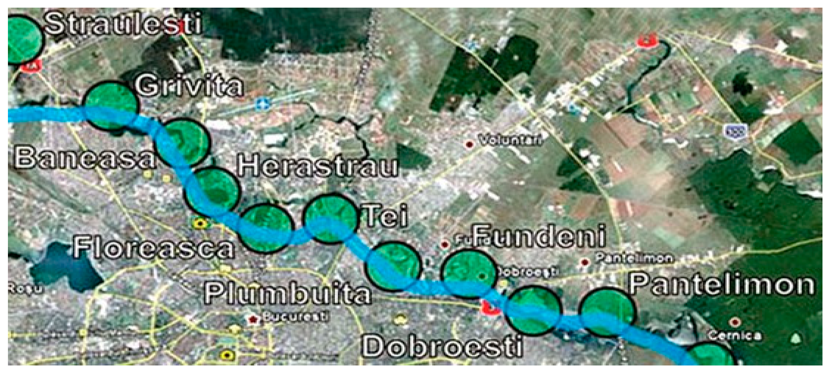
• Lakes over the Colentina River: Străuleşti, Griviţa, Băneasa, Herăstrău, Floreasca, Tei, Colentina, and Pantelimon;
• Lakes inside some parks: Tineretului, Circului, Cişmigiu, and Titan;
• Morii Lake, organized on Dâmboviţa River, having the purpose to regularize its flow.

The location of these lakes on the map of Bucharest is illustrated in Figure 1, while their important characteristics are displayed in

Table 1. Main characteristics of monitored lakes [45].

No	Lake	Surface Area, ha	Volume, mil m3	Depth, m
1	Străuleşti	33.0	0.70	1–5
2	Griviţa	53.0	l.00	1–4
3	Băneasa	40.0	0.60	1–3
4	Herăstrău	74.0	l.50	1–5
5	Floreasca	70.0	1.60	1–5
6	Tei	80.0	1.70	1–5
7	Pantelimon II	260.0	3.20	1–6
8	Tineretului	13.0	0.20	1–6
9	Lacul Titan I	1.8	0.04	1–3
10	Lacul Circului	1.0	0.02	1–4
11	Lacul Cişmigiu	2.9	0.04	1–2
12	Lacul Morii	246.0	14.70	10

.

The riverbed of the Dâmboviţa and Colentina Rivers is formed with sand and gravel, and the banks of the river are covered with concrete slabs, while the lakes from parks are arranged on swampy zones.

The climate in Bucharest is temperate continental, and topoclimate is lacustrine. The monthly and annual averages of temperature in Bucharest, at Filaret station, are presented in

Table 2. Monthly average temperature of the air in Bucharest, calculated during the period 1901–2000 [46].

Month	I	II	III	IV	V	VI	VII	VIII	IX	X	XI	XII	$\overline{\mathit{T}}$
T [°C]	−2.2	−0.2	5.3	11.6	16.9	20.7	22.9	22.4	17.7	11.8	5.5	0.4	11.0

.

The values for the monthly averages of rainfall in the lake areas measured in two meteorological stations, at Băneasa and Dragomireşti Vale, are presented in

Table 3. Monthly and annual average rainfall, mm/m².

Station/Month	I	II	III	IV	V	VI	VII	VIII	IX	X	XI	XII	Mean
Băneasa	29.4	26	32.2	40.8	63.5	92.4	69.2	49.8	39	39.3	42.5	31.0	555.3
Dragomireşti Vale	31.7	22.1	37.9	40.5	64.9	85.5	57.7	49.7	48.1	38.5	36.5	32.0	545

.

The analyzed lakes are artificial, and they are the result of water stream barrage. They appeared from regularization needs or in recreation areas. The industrial pollution has been significantly reduced since most of industrial units in this area are closed. So, an increasing pollution source is provided by buildings, usually chaotically placed or organized in chains of residential districts, with rather precarious systematization and sewage. The lake areas still remain frequent waste deposit sites, from small productive units or from population. The lakes from the parks are less exposed to pollution.

2.1. Heavy Metals Data

The main pollution source with Pb²⁺ and Hg²⁺ is represented by particulate matter (PM) from the atmosphere, which falls on the free surface of water [47,48,49,50]. As a result, the quality of waters in Bucharest area, Colentina River, and surrounding lakes, is inadequate, due to the wastewater discharge upstream the river from industrial units and domestic sewage. The main pollution trend is represented by high organic content and heavy metals.

The analyses for the concentration of Pb²⁺ and Hg²⁺ ions in surface waters of Bucharest area and the identification of their pollution sources are presented in the following:

The concentration of ions of Pb²⁺ and Hg²⁺ in the lakes analyzed has been daily monitored during the period March 2007–November 2009, except for wintertime, when they were dried or frozen.

The water sampling for each lake has been performed as follows (according to standard procedures):

• Daily at one meter far from the bank, in at least 5 places in the same spatial-temporal conditions;
• In half liter recipients of single-use, made of P polyethylene, specially produced for water sampling;
• The samples were analyzed daily in specialized laboratory by using AAnalyst 700 Atomic Absorption Spectrometer, Perkin Elmer, Waltham, USA and a Direct Mercury analyzer, DMA 80, Milestone, Shelton, USA for lead and mercury, respectively.

2.2. Nitrates and Phosphates Data

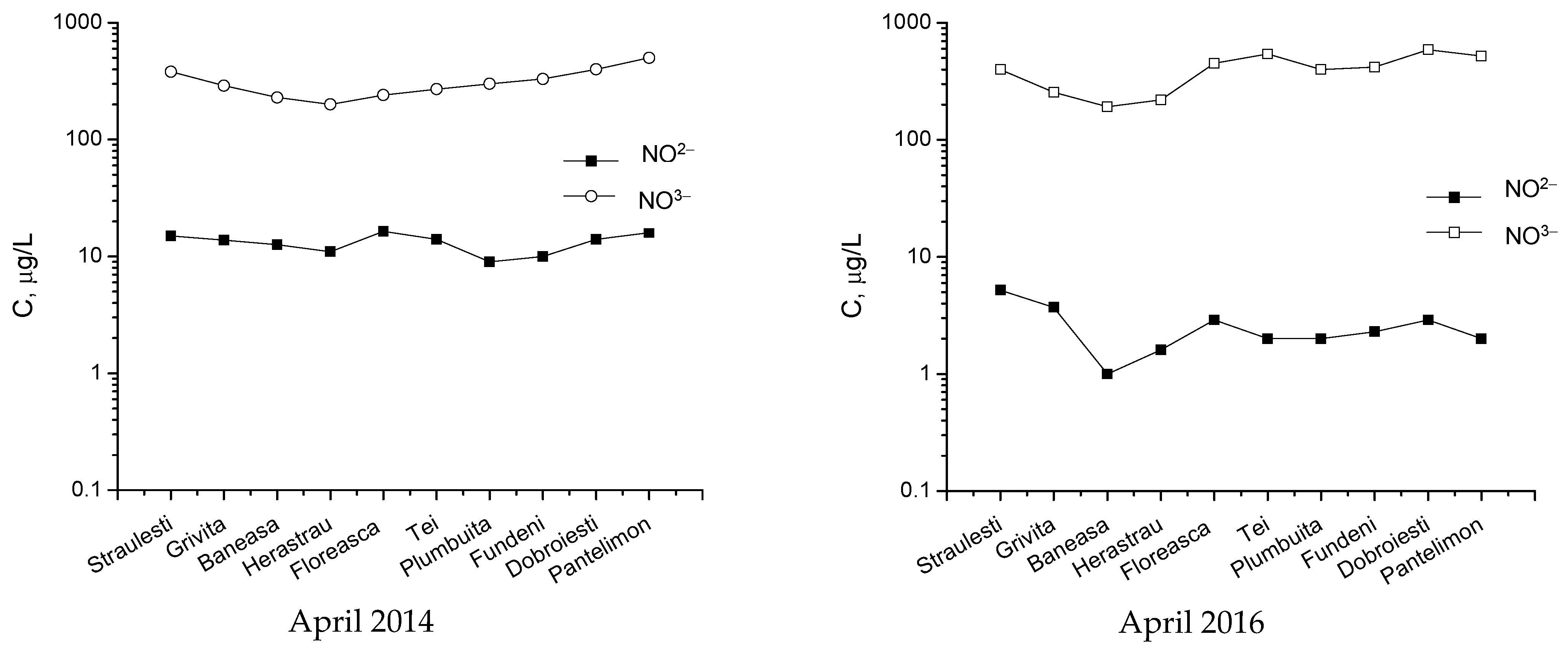
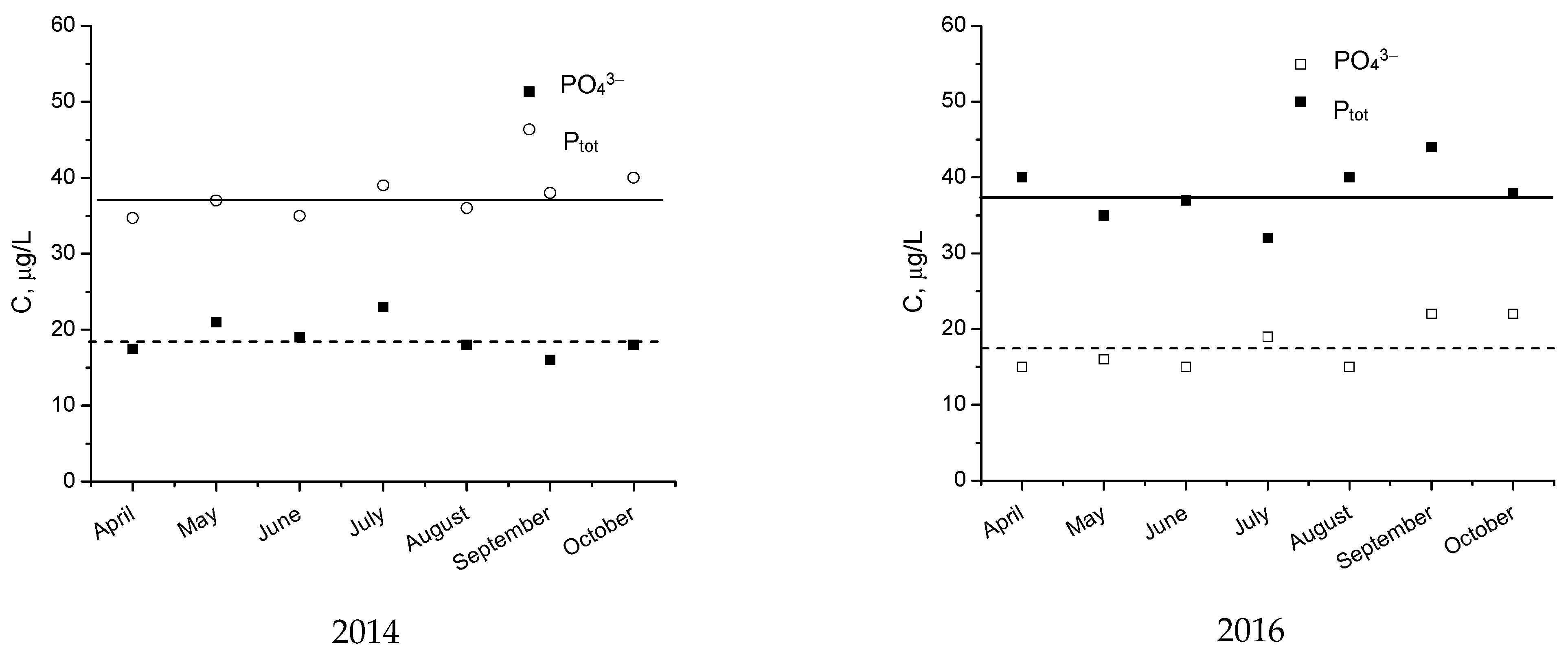
Data resulting from concentration monitoring of ions NO₂⁻, NO₃⁻, PO₄³ ⁻, and P_tot in surface waters from Bucharest during the 2013–2016 period are presented and analyzed.

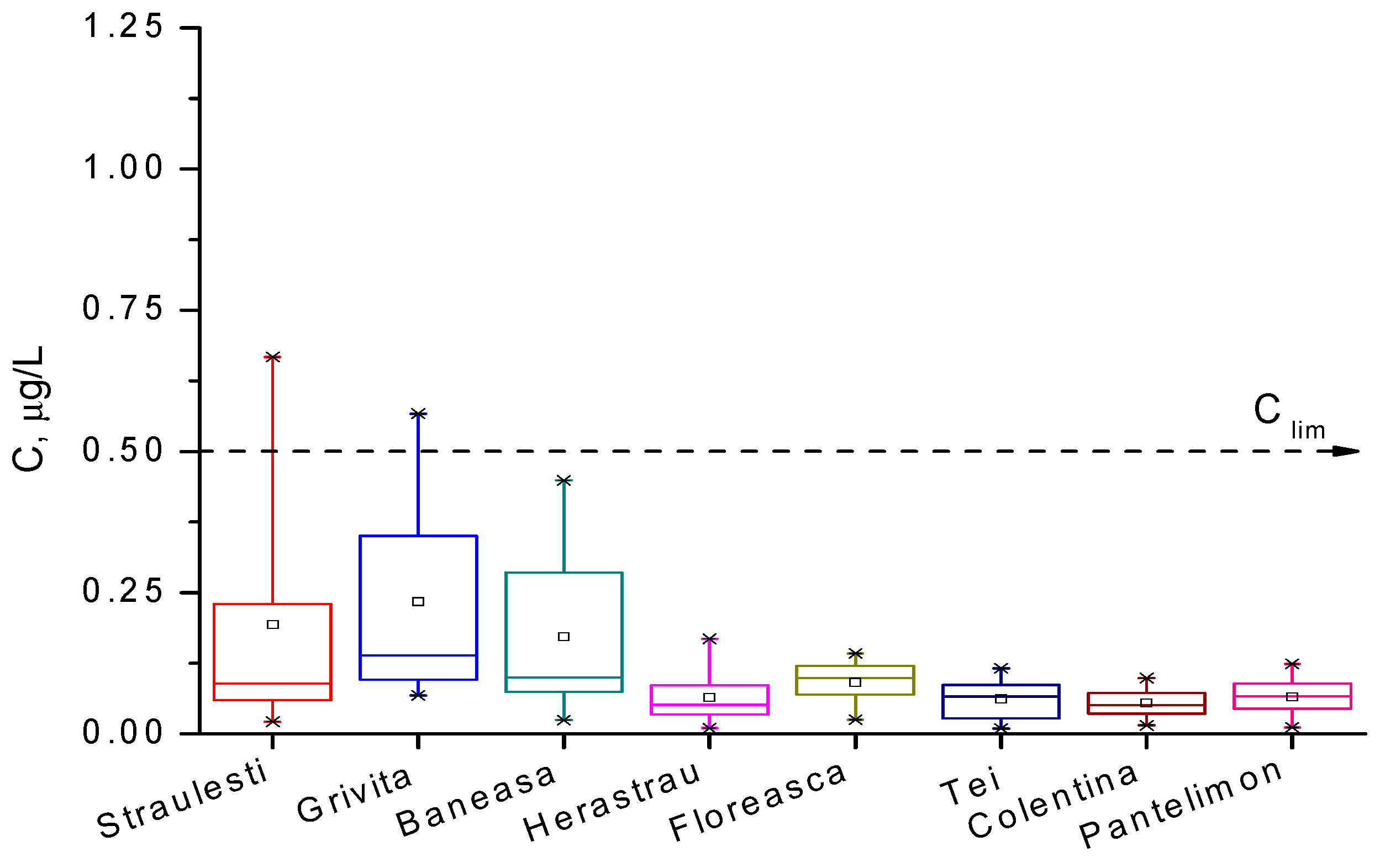
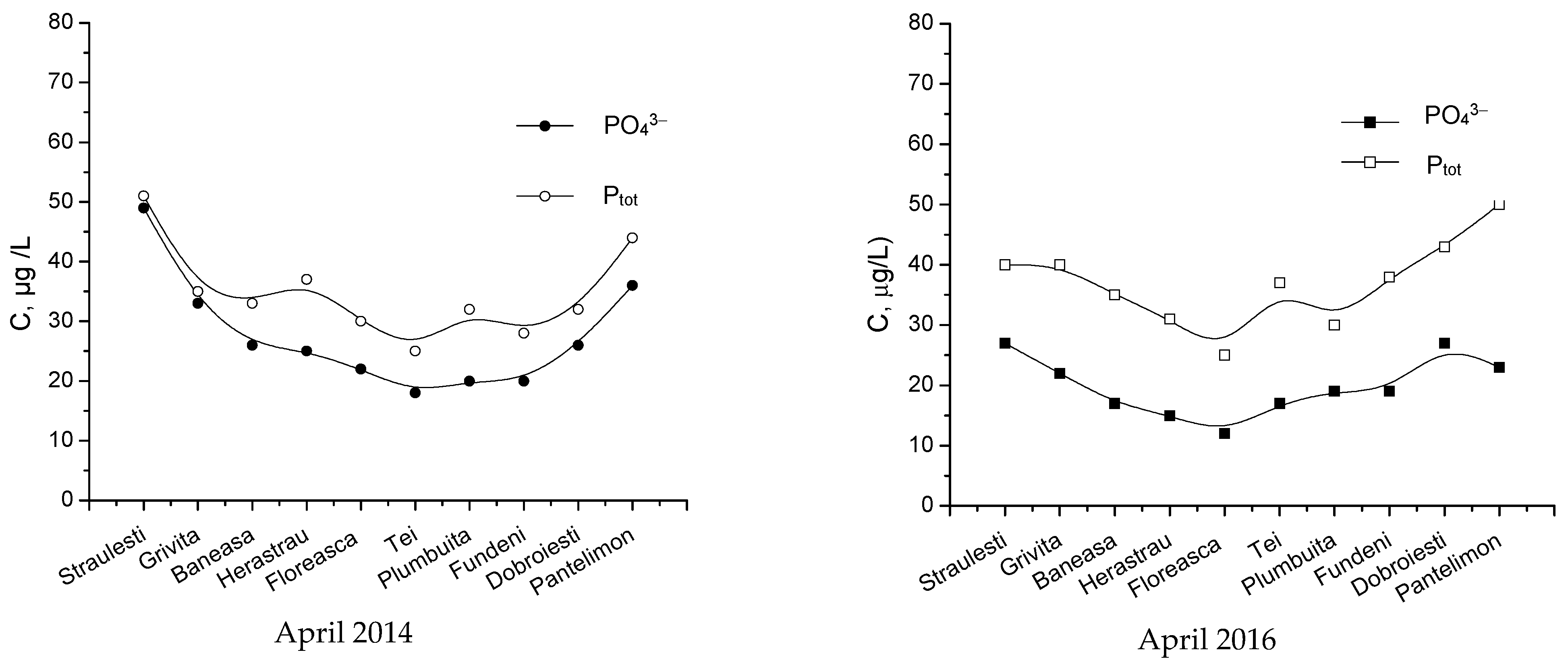
A measure of the degree of the eutrophication of the lakes is represented by the concentrations of these ions. The surface waters which are monitored are that of 10 lakes resulting from Colentina River systematizing (Figure 2). The sources of pollution with nitrates and phosphates are coming from economic activities around lakes, urban transport, and the initial pollution of Colentina River.

A direction of data analysis aims to establish whether there is a significant statistical difference between concentrations of these pollutants in surface waters analyzed.

3. On the Results

In this section, the statistical results and their interpretation are presented, together with the experimental conclusions that can be drawn.

3.1. Lead Pollution Data Analysis

The concentrations of Pb²⁺ ions within the analyzed waters are presented and compared in the box diagrams in Figure 3 and Figure 4 and quantified in

Table 4. Maximal concentration of lead in 2007–2009 period within the monitored lakes.

Lake No.	1	2	3	4	5	6	7	8	9	10	11	12
cPb, μg/L	1.22	1.29	1.01	0.96	0.57	0.67	0.72	0.69	0.91	0.57	0.56	1.27

. One can remark that the lead pollution is not a serious problem in most of the waters around Bucharest, except for the lakes numbered with 1, 2, 3, and 12 in the Table 1, where the concentrations are accidentally above 1 µg/L. The content of pollutants in the water of the Colentina River is rather high upstream of the entrance to Bucharest, and it is diminished via natural dilution in the surroundings lakes denoted with 4, 5, 6, 7, and 9. As expected, the lakes inside parks, such as 8, 10, and 11, present a smaller content of lead, while lakes 1, 2, and 12 are the most polluted. The distribution of Pb²⁺ concentration in all cases is not symmetrical, suggesting that this concentration shows a periodic character.

These results lead to the conclusion that the main pollution source with Pb²⁺ in the Bucharest area is due to particulate matter from air that is deposited on the water surface of lakes [50].

One can observe that other pollution sources remained, although leaded petrol has no longer been commercialized since August 2005. These sources are emission gasses from fossil fuel combustion used in thermal or electrical power plants and from vehicles. Another important source is represented by the numerous demolitions and rehabilitations of degraded buildings, which produce an important quantity of dust with lead content. Furthermore, the waste of these works is chaotically disposed into lake water, causing significant pollution.

The statistical analysis of the experimental data, which are sampled from one of the most polluted lakes, number 2, Griviţa, is illustrated in the Shewhard monitoring diagram in Figure 5. The central line of the diagram, CL, is the arithmetic average of the measured values, and the upper attention limit, UAL, was calculated with the rule 3σ. The diagram points out that UAL is systematically higher; in some cases, the maximum admitted limit is also overcome. In this case, it is obvious that the process is not controllable by statistical methods.

The CUSUM diagram in Figure 6, for the data analyzed in Figure 5, proves that the general trend of data is decreasing, and it oscillates periodically. Consequently, the trend of data is calculated, and this is represented in Figure 7. As one may observe, the data have an insignificant decreasing trend, demonstrating that the target value within the CUSUM diagram has been not correctly established.

The periodic character illustrated by the oscillating trend shown in Figure 6 is proven using the correlation of data with sine wave model, presented in Figure 8. The equation of this model, obtained via nonlinear regression, has the form:

$$c=0.295+0.68\cdot \sin \left(\frac{2\cdot \mathsf{\pi }\cdot t}{7}+5.51\right)$$

(1)

The relation (1) demonstrates the periodic character of lead concentration change, with a 7-day period. The weekly variation of lead content shows that it is related to the intensity of road traffic: more intensive during the week and lower at weekend. The position of the motorway near the Griviţa and Morii Lakes proves that the main lead pollution source is provided by vehicles using diesel oil, while the lakes inside the parks are less polluted.

3.2. Mercury Pollution Data Analysis

For the analyzed water samples, the concentrations of Hg²⁺ ions are presented in box diagrams in Figure 9 and Figure 10, comparatively, and they are quantified in

Table 5. Statistical parameters for the concentration of mercury ions in Griviţa lake during the period March–July 2009.

Statistical Parameter	Value
Mean	0.245
Standard error	0.011
Median	0.212
Standard deviation	0.140
Kurtosis	0.663
Skewness	1.010
Range	0.705
Confidence level (95.0%)	0.022

. We observe that mercury ion pollution is not a serious problem in most waters around Bucharest, except for the Străuleşti and Griviţa Lakes, where the concentrations are accidentally above 0.5 µg/L. The content of the pollutant in the water of the Colentina River is rather high upstream of the entrance to Bucharest, and it is diminished in the surrounding lakes via natural dilution. Lakes inside parks, such as Cişmigiu, Circului, Titan, and Tineretului, exhibit a lower metal content, as expected, while Morii Lake is among the most polluted surface waters in the Bucharest zone. The distribution of the concentration of Hg²⁺ ions is, in all cases, asymmetrical, suggesting that the time evolution of this indicator presents a periodic character. These findings lead to the conclusion that in the Bucharest territory, the main source of pollution with Hg²⁺ is represented by particulate matter from air that is deposited on the surfaces of lakes. The principal sources of PM in air are the gases emitted from fossil fuels combustion in thermal or electrical power plants and vehicles. The numerous demolitions and rehabilitations of old buildings produce a huge source of dust with heavy metal content; these are another important source of mercury pollution. Unfortunately, the wastes from these works are chaotically disposed near or into lake water, causing them a significant degradation. Also, the rainfall over agriculture lands treated with organomercury compounds provides other pollution causes in the areas of the Străulesţi and Griviţa Lakes.

Figure 11 shows the result of a statistical analysis for the experimental data sampled from Griviţa Lake, which is one of the most polluted surface waters in Bucharest, where the Shewhard monitoring diagram is illustrated. The central line of the diagram (CL) is the mean of the values measured, and the upper attention limit (UAL) has been computed with the rule 3σ. The diagram highlights that UAL is higher than the limit concentration and this implies that the process is out of statistical control, as is proven also via the value of process capability index, $C_p$, defined using [51,52]

$$C_p=\frac{C_{lim}-CL}{UAL-CL}=0.62<1,$$

which should be higher than unity for a process under statistical control.

At the same time, one can notice that the concentration of Hg²⁺ ions within Griviţa Lake is periodically higher than the upper admitted limit, $C_{lim}$.

It can be demonstrated that the Hg²⁺ monitored concentrations form a nonstationary time series, since they exhibit an increasing trend and periodicity [53,54], as illustrated in Figure 12 and Figure 13. If the trend and the periodicity are removed from the initial data, a novel time series based on fluctuations only is formed [35,37]. The box diagram from Figure 14 reveals that fluctuations have a symmetrical distribution for which the median and mean values are the same [36]. As a result, the fluctuation distribution can be approximated with a normal distribution.

The X and R diagrams in Figure 15 and Figure 16 prove that, from the fluctuation point of view, the monitored process is under statistical control [42].

3.3. Nitrates and Phosphates Data Analysis

This data analysis searches to establish if there is a significant statistical difference between the concentrations of these pollutants in analyzed surface waters. For this reason, the t test applied for two samples, considering different variances, using Excel program, was performed, and the results displayed in

Table 6. t test with different variances to test the equality of the monthly means for dimensionless concentration of PO₄³⁻ in surface waters from Bucharest—April 2014.

t-Test: Unequal Variances for April 2014 Data
Lakes	1–2		1–3		1–4		1–5		1–6
Mean	0.31	0.44	0.31	0.34	0.31	0.33	0.31	0.53	0.31	0.57
Variance	0.22	0.14	0.22	0.15	0.22	0.24	0.22	0.14	0.22	0.16
Observations	4.00	4.00	4.00	4.00	4.00	4.00	4.00	4.00	4.00	4.00
Hypothesized Mean Difference	0.00		0.00		0.00		0.00		0.00
df	6.00		6.00		6.00		6.00		6.00
t Stat	−0.43		0.81		0.80		−0.41		−0.81
t Critical two-tail	2.45		2.45		2.45		2.45		2.45
Lakes	1–7		1–8		1–9		1–10
Mean	0.31	0.35	0.31	0.31	0.31	0.45	0.31	0.43
Variance	0.22	0.15	0.22	0.17	0.22	0.24	0.22	0.17
Observations	4.00	4.00	4.00	4.00	3.00	5.00	3.00	5.00
Hypothesized Mean Difference	0.00		0.00		0.00		0.00
df	4.00		4.00		4.00		4.00
t Stat	0.22		0.53		0.44		0.17
t Critical two-tail	2.45		2.45		2.45		2.45

and

Table 7. t test—unequal variances of monthly mean of dimensionless concentration of PO₄³⁻ in surface waters from Bucharest—April 2016.

t-Test: Unequal Variances for April 2016 Data
Lakes	1–2		1–3		1–4		1–5		1–6
Mean	0.37	0.42	0.37	0.58	0.37	0.33	0.37	0.53	0.37	0.57
Variance	0.21	0.14	0.21	0.22	0.21	0.24	0.21	0.14	0.21	0.16
Observations	5.00	5.00	5.00	5.00	5.00	5.00	5.00	5.00	5.00	5.00
Hypothesized Mean Difference	0.00		0.00		0.00		0.00		0.00
t Stat	−0.18		0.08		−0.63		0.10		−1.03
t Critical two-tail	2.31		2.31		2.31		2.31		2.31
Lakes	1–7		1–8		1–9		1–10
Mean	0.37	0.35	0.37	0.31	0.37	0.45	0.37	0.43
Variance	0.21	0.15	0.21	0.17	0.21	0.24	0.21	0.17
Observations	5.00	5.00	5.00	5.00	5.00	5.00	5.00	5.00
Hypothesized Mean Difference	0.00		0.00		0.00		0.00
t Stat	0.04		0.05		−0.77		−0.78
t Critical two-tail	2.31		2.31		2.31		2.31

prove that the pollution degree of the lakes are similar in April 2014 and April 2016, respectively. The statistical analysis demonstrates that, for the lake water coming from the same river, i.e., Colentina River, there is no other significant source of pollution with these two kinds of pollutants.

The data represented in Figure 17 and Figure 18 present the concentration variations for monitored pollutants within the considered lakes around Bucharest in April 2014 and 2016, respectively. Although these data show some variations from one lake to another, statistical tests have proven that these differences are insignificant. However, in all the presented cases, the first lake (Străuleşti) and last lake (Pantelimon) have higher concentrations of nitrates and phosphates due to nutrients used in the agricultural activity in those zones.

The data presented in Figure 19 form a stationary time series since they have been collected at a regular interval (monthly), and the statistical properties are independent of time. This means, in particular, that the data have constant mean and variability constant over time for the time series. The time series has a horizontal pattern shifting to a new level if additional sources of pollutants appear. The data pattern is an important factor to understand how the time series has behaved in the past. If such behavior can be expected to continue in the future, the past pattern can be used to select an appropriate forecasting method. The data from Figure 19 show a time series with a horizontal pattern, since the data fluctuate around the constant mean and present random variability. The average values or means for this time series are 18.8 and 37.5 mg/L for PO₄³⁻ and P_tot, respectively, in 2014, and 17.9 and 37.2 mg/L for PO₄³⁻ and P_tot, respectively, in 2016.

Forecasts for the time series from this paper involve an approach that uses the most recent value as the forecast for the next month—the simplest forecasting method. The forecasts obtained for the historical data are shown in

Table 8. The forecasts obtained for the historical data.

2014
	Experimental Data		Forecast Data		Forecast Error, %
	PO43−	Ptot	PO43−	Ptot	PO43−	Ptot
April	17.5	34.7	-	-	-	-
May	21.0	37	17.5	34.7	16.67	6.22
June	19.0	35	21	37	10.53	5.71
July	23.1	39	19	35	17.39	10.26
August	18.2	36	23	39	27.78	8.33
September	16.1	38	18	36	12.50	5.26
October	18.0	40	16	38	11.11	5.00
Mean forecast error					16.00	6.80
2016
April	15	40
May	16	35	15	40	6.25	14.29
June	15	37	16	35	6.67	5.41
July	19	32	15	37	21.05	15.63
August	15	40	19	32	26.67	20.00
September	22	44	15	40	31.82	9.09
October	22	38	22	44	0.00	15.79
Mean forecast error					15.41	13.37

in the column Forecast Data, and the measurements of the accuracy of this forecasting method are able to reproduce the time series data with a mean forecast error greater than 10%.

The second forecasting method for the time series uses the average of all the historical data available as the forecast for the next period. This starts by developing a forecast for the second month. Because it is only one historical value available before the second month, the forecast for the second month is only the time series value for the first month. To calculate the forecast for the third month, it takes the average values for the first two months. Thus, for every measure, the average of past values provides more accurate forecasts than those from the first method. In general, if the representative time series is stationary, the average of all the historical data always provides the best results. These are presented in

Table 9. The forecasts obtained with the mean of the historical data.

2014
	Experimental Data		Forecast Data		Forecast Error
	PO43−	Ptot	PO43−	Ptot	PO43−	Ptot
April	17.5	34.7	17.50	34.7	0.00	0.00
May	21	37	19.25	35.85	3.11	3.11
June	19	35	19.17	35.57	1.62	1.62
July	23	39	20.13	36.43	6.60	6.60
August	18	36	19.70	36.34	0.94	0.94
September	16	38	19.08	36.62	3.64	3.64
October	18	40	18.93	37.10	7.25	7.25
Mean forecast error					3.31	3.31
2016
April	15	40	15	40	0.00	0.00
May	16	35	15.50	37.50	3.13	7.14
June	15	37	15.33	37.33	2.22	0.90
July	19	32	19.50	38.50	2.63	20.31
August	15	40	16.00	36.80	6.67	8.00
September	22	44	17.00	38.00	22.73	13.64
October	22	38	17.71	38.00	19.48	0.00
Mean forecast error					8.12	7.14

. In this second case, the mean forecast error is less than 10%.

Important factors in comparing different forecasting methods are represented by the measures of forecast accuracy, but we have to be careful not to rely upon them too much. To select a forecasting method, good judgment and knowledge about environmental conditions that might also affect the prevision should be carefully taken into account. The historical forecast error is not the single condition, particularly when the time series is likely to change in the future.

4. Discussion

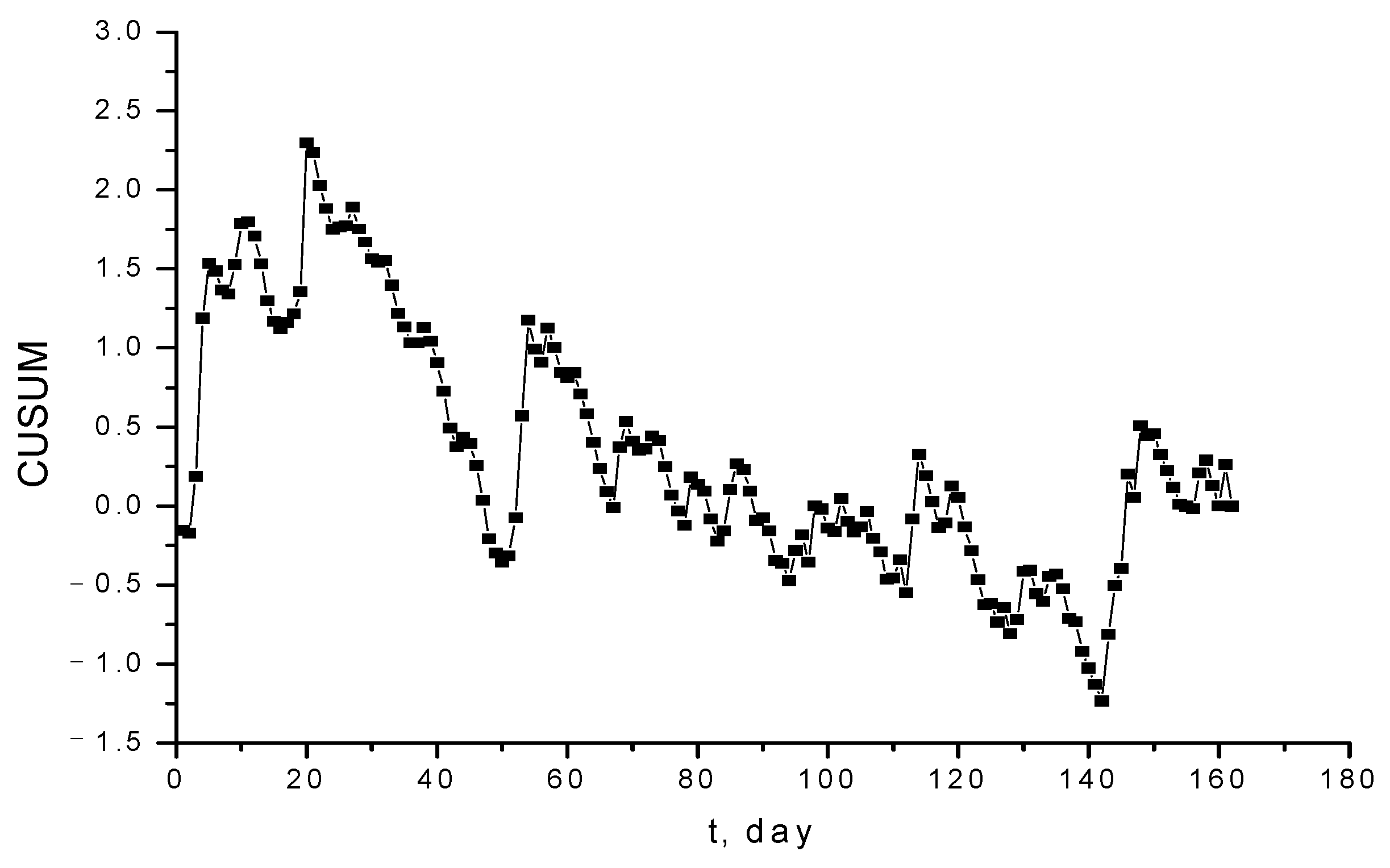
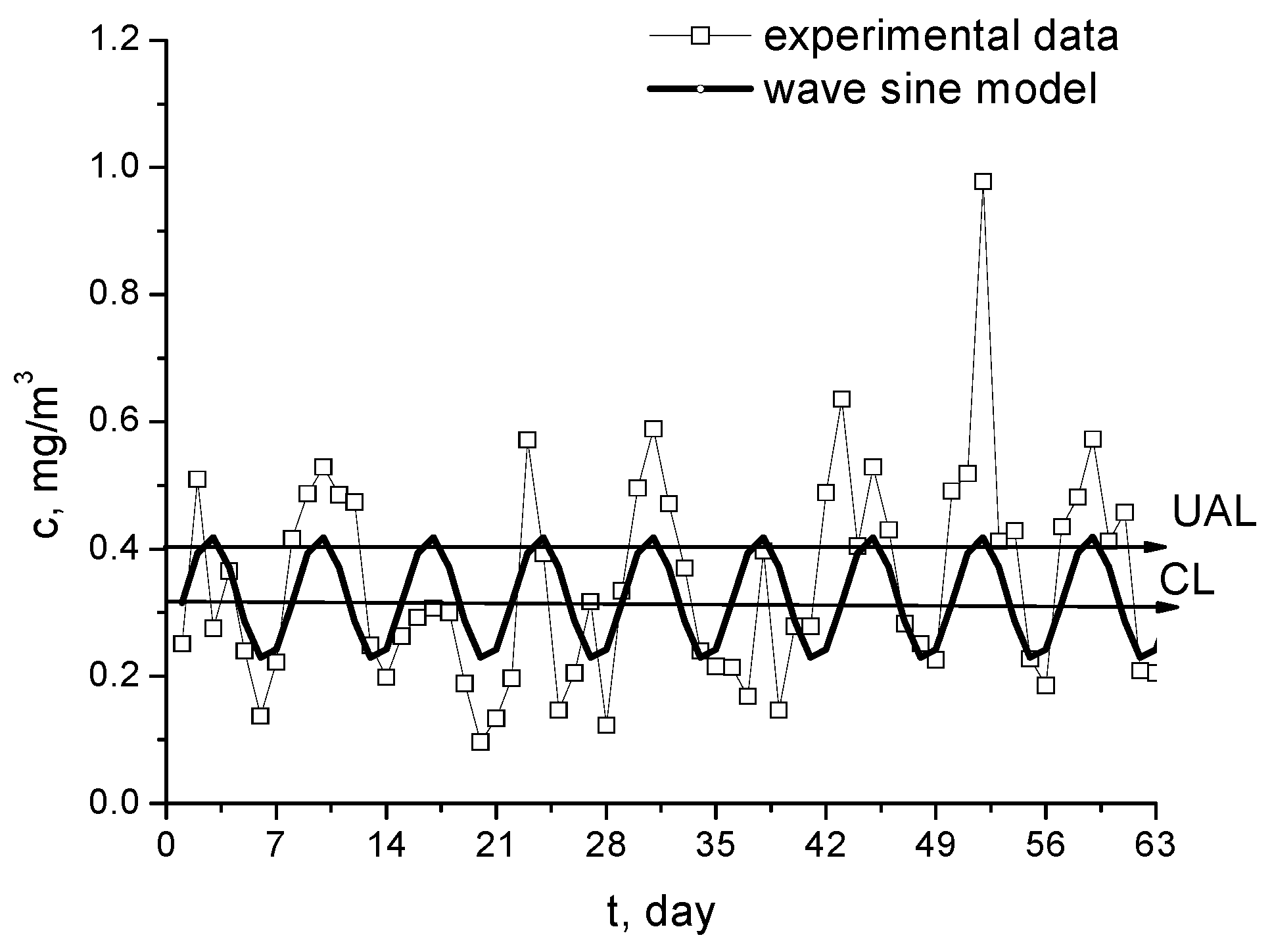
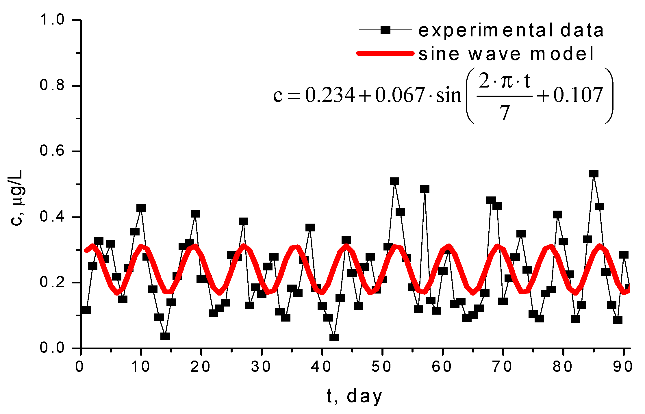
The daily registration of concentrations for lead and mercury in surface waters forms a univariate time series that consists of observations that have been recorded sequentially over equal time intervals. Such time series have periodicity that represents sinusoidal fluctuations over entire weeks and seasonality over the year. The seasonal pattern is consistent with a wave sine model. The autocorrelation function has been used to obtain the autocorrelation structure property of the series.

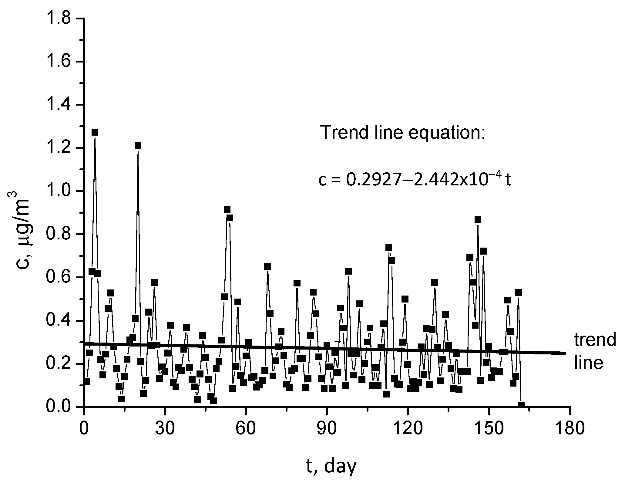
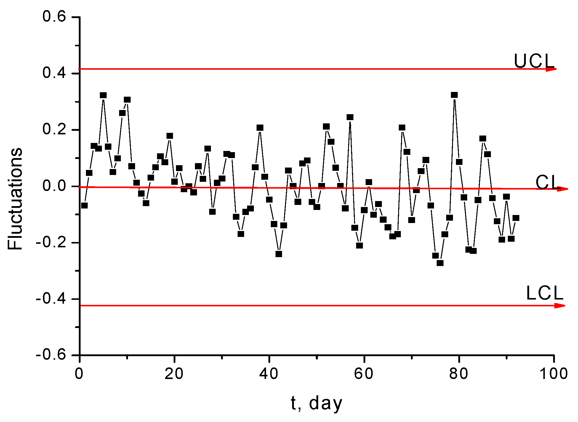
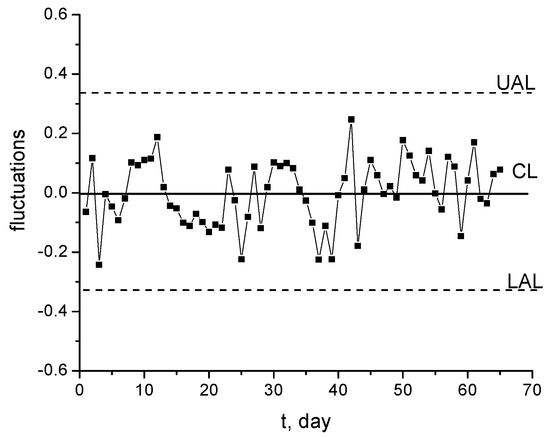
In the case of the first set of data (lead emissions), which shows a trend and periodicity, monitoring diagrams are built based only on concentration fluctuations obtained after the removal of trend and periodicity from the initial data [35].

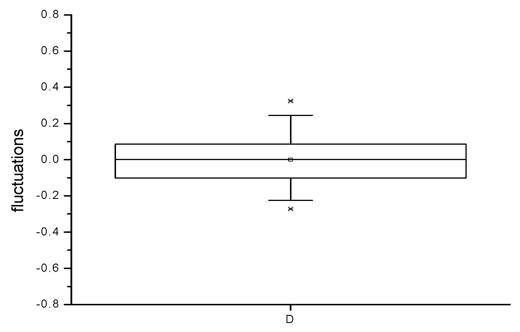
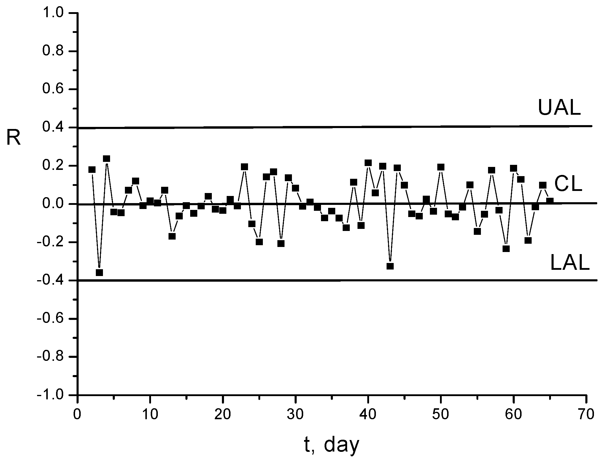
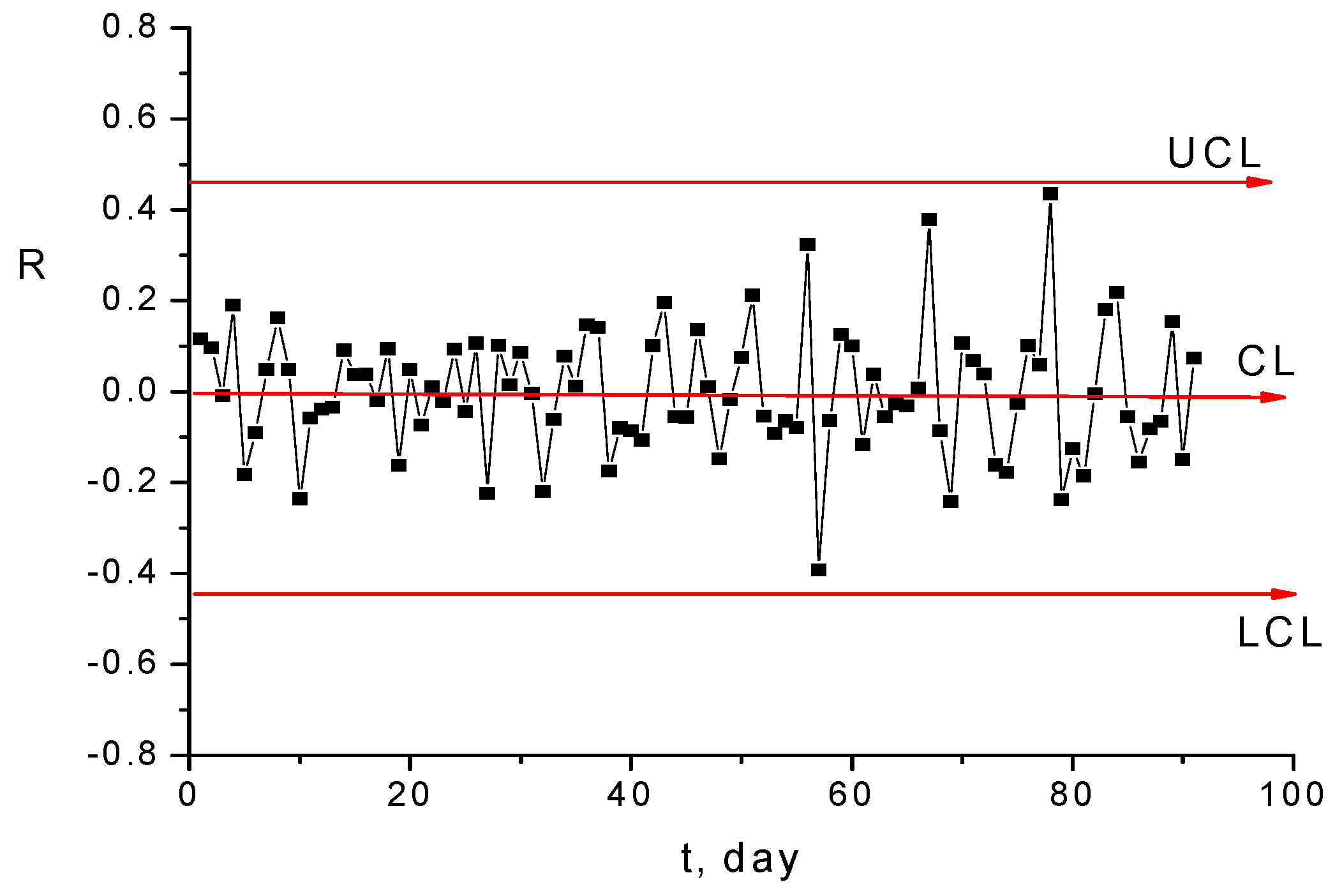
The results represented in Figure 20 and also the range diagram from Figure 21 prove that the experimental measurements can be statistically monitored with a diagram of Shewhart type. The diagram R of the range (amplitudes) of fluctuation variations confirms that these are within the limits of statistical control of the process.

Monitoring and statistics for the concentrations of lead ions in surface waters from Bucharest zone showed the following aspects:

• The maximum admitted limit of Pb²⁺ concentration is sometimes overcome in several lakes exposed to traffic pollution or waste disposal;
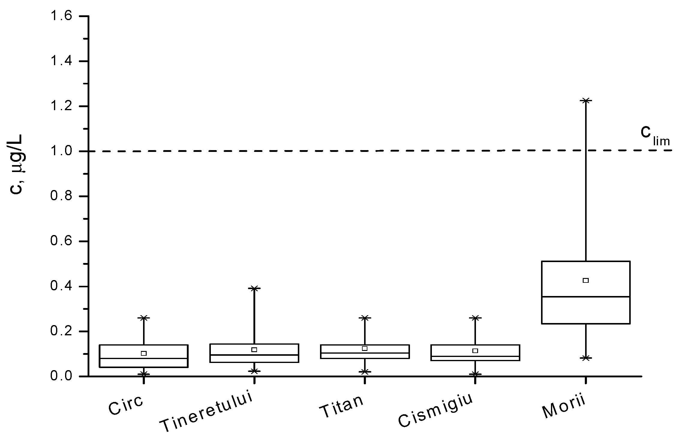
• The lakes situated inside the parks are less polluted;
• The daily Pb²⁺ concentrations present a decreasing trend for all the studied cases, and they have a weekly periodic character;
• Shewhart type monitoring diagrams X and R can be involved to monitor these data, but only for concentration fluctuations prepared by removing trend and periodicity from the initial data;
• The surface water pollution with lead in the Bucharest area is quite small and caused mainly via PM from air as the result of the combustion processes, demolition, and rehabilitation of degraded buildings.

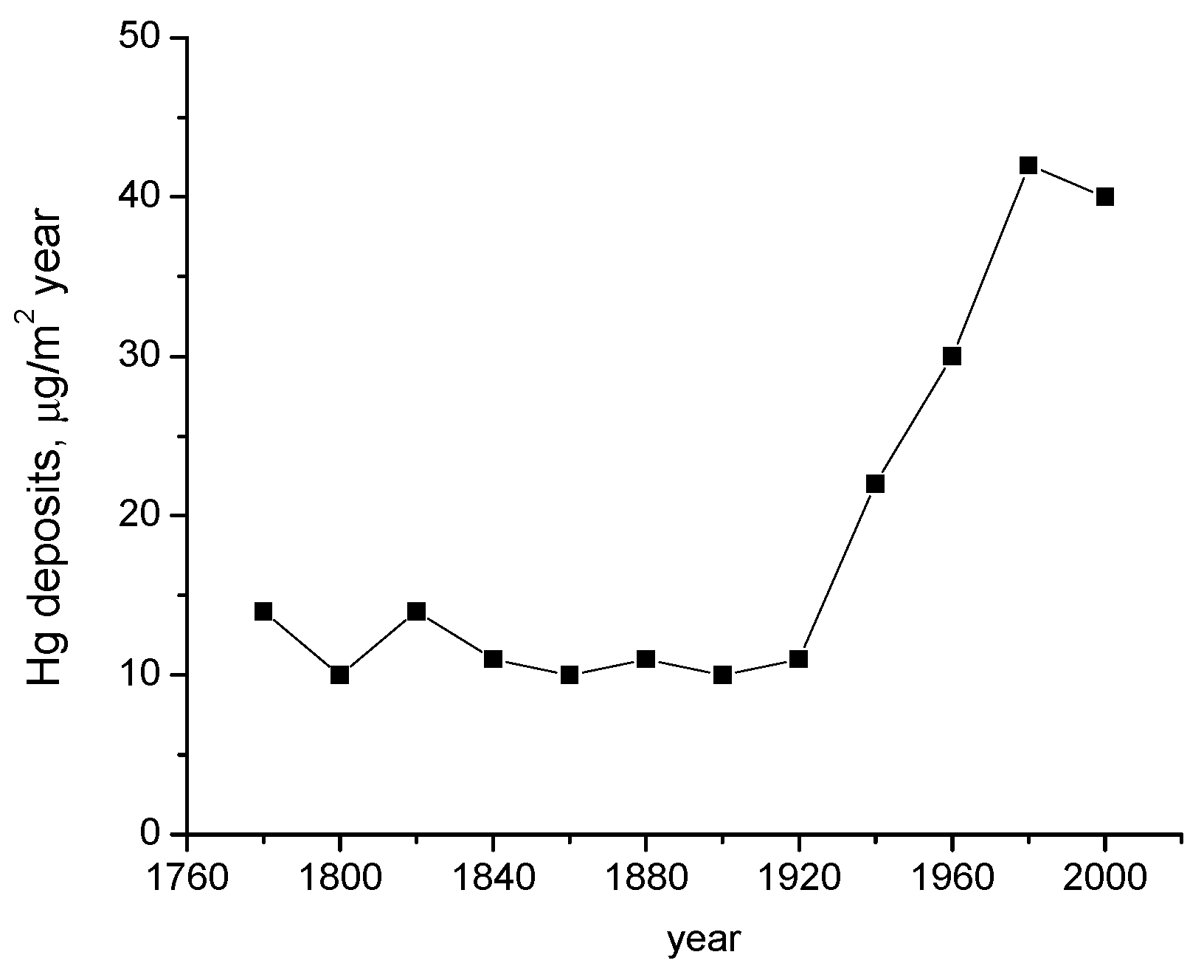
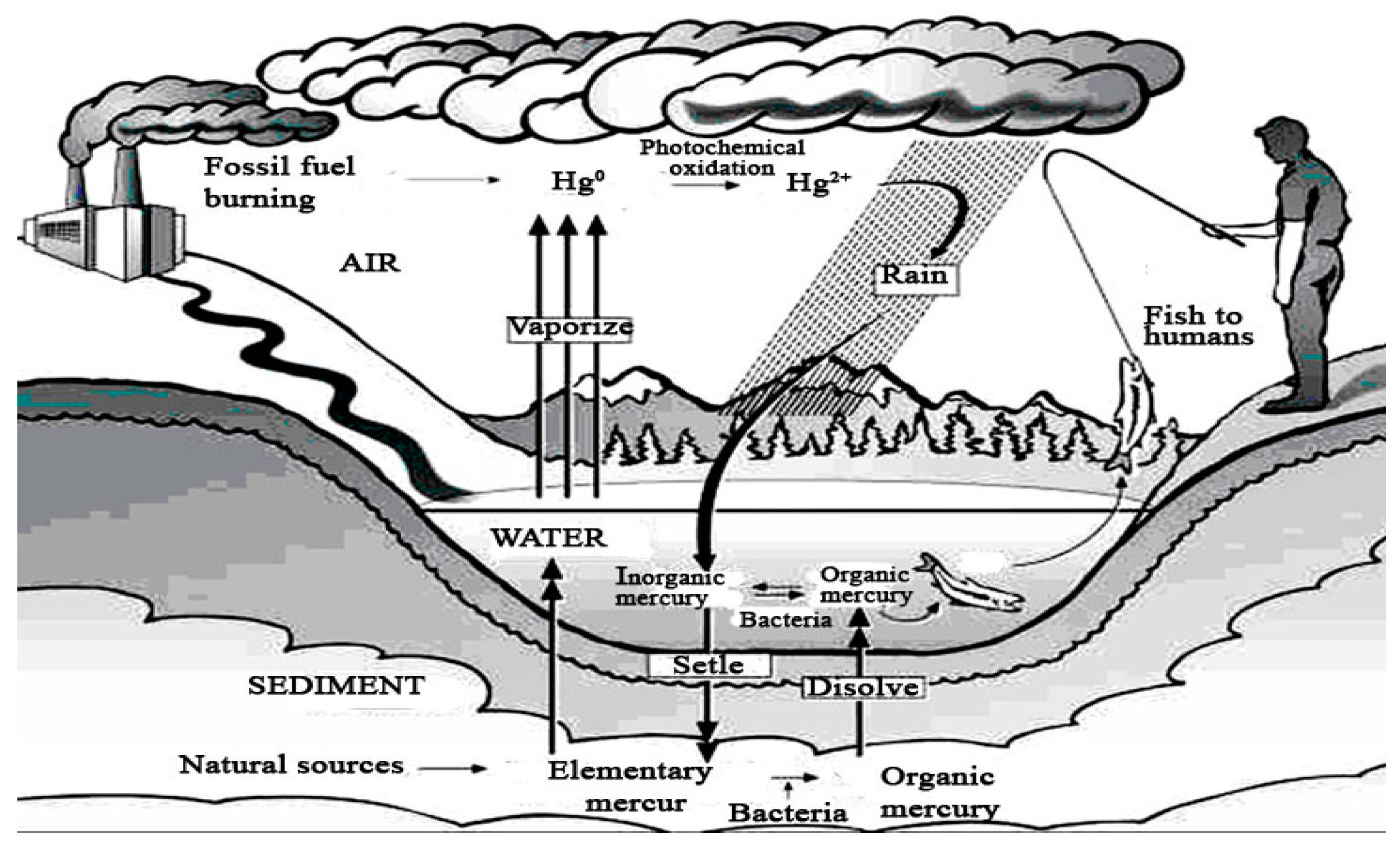
At present time, the reported level of global mercury contamination is growing, having various harmful effects on the atmosphere, aquatic, and terrestrial environment. From Figure 22 results the increasing amount of mercury in the environment that follows the trend of industrial development. A big part of mercury compounds provided via anthropogenic activity is released into the atmosphere, whence they are transported and transferred on water surface and soil. The mercury present under various chemical forms is highly accumulated in sediments and living organisms in the aquatic medium, as it is illustrated in the image of mercury circuit around environmental factors in Figure 23. 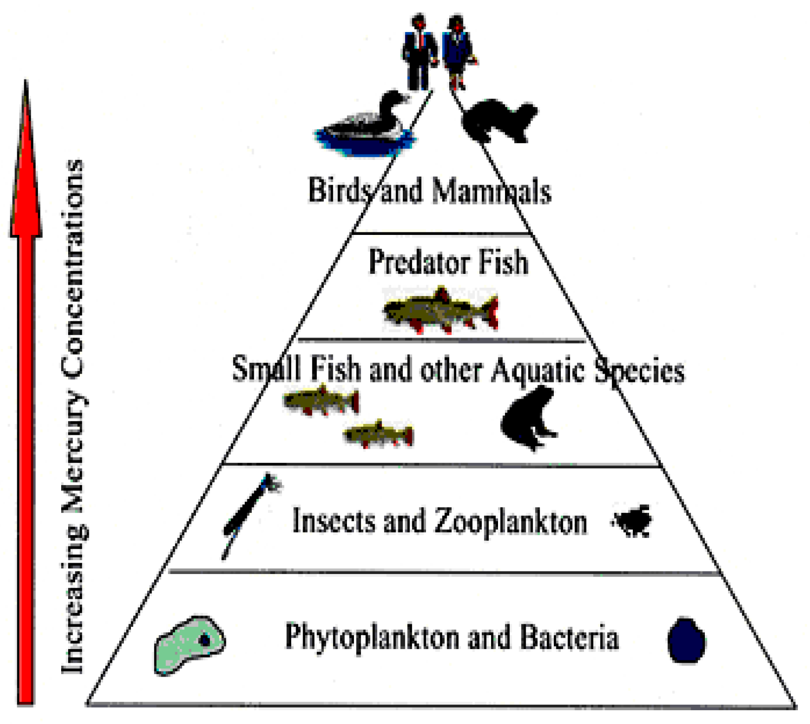In accordance with EPA studies [55], mercury is bio-accumulated from the aquatic medium into food, and then it is bio-concentrated into human body (Figure 24).

The main source of mercury uptake in the human body is represented by contaminated food, especially fish. Methylmercury can bio-concentrate to 1 part per million, a level found in some top predators like tuna, swordfish, and shark, that means a million-fold increase, in water containing 1 to 10 parts of mercury per trillion parts of water.

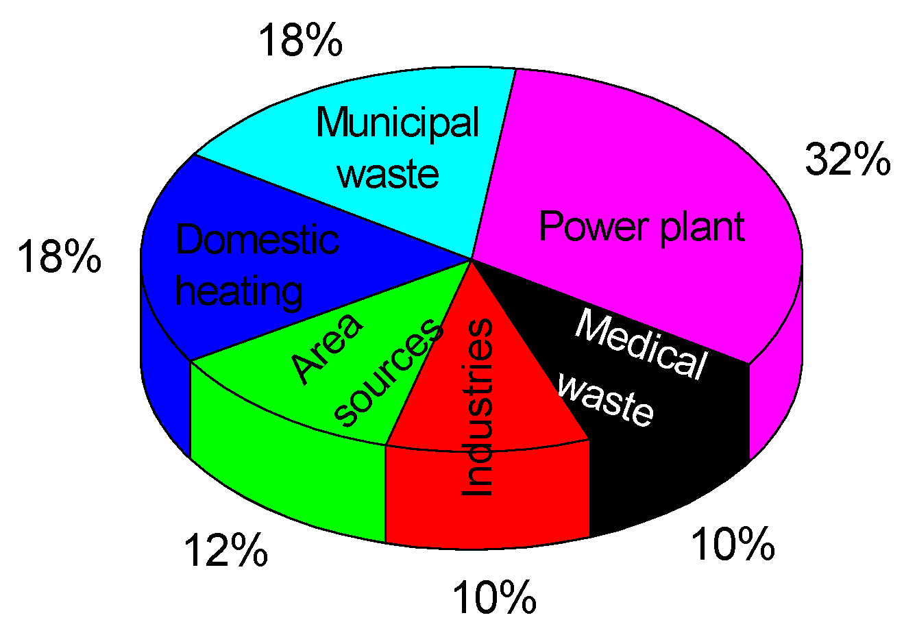
From the pie diagram shown in Figure 25, the main pollution source with mercury of the atmosphere, and implicitly of surface water and soil, is represented by gases released from fuel combustion in thermal power plants and building heating, as can be seen.

In the chemical industry, in the fabrication of caustic soda, dyes, paper, some pesticides and fungicides, pharmaceutic products and disinfectants, etc., mercury is frequently used. These industries are potential pollution sources with mercury, both by means of their wastes and of the products used in other industries. The inappropriate use of organomercury fungicides in the various phases of agriculture works could cause the poisoning of birds and animals, the contamination of soil, and transfer into the aquifer.

Vehicles using petrol or diesel oil release burning gases containing heavy metals such as lead, mercury, and cadmium (this last heavy metal has been also sampled and analyzed in the laboratory, but, the obtained concentration values being too small, the continuation of its study did not show any importance). It is considered that the mercury generated by road traffic represents cca 3% of the total amount released into the atmosphere from various sources; it is included in the sector of ‘Area sources’ in Figure 25.

Severe measures have been taken to limit the use of organic mercury compounds in the paper industry and agriculture, by restricting the discharge of waste or banning fishing in some polluted areas, as a result of the awareness of the potential dangers caused via the mercury pollution of the ecosystem.

The weekly doses temporarily admitted are 0.3 mg total Hg per person, out of which less than 0.2 mg can be methylmercury, CH₃Hg⁺ (expressed in mercury), which corresponds to 0.005 mg and 0.0033 mg/kg body, in accordance with the recommendations of the Expert Committee on Food Additives of FAO/OMS. A concentration of approx. 0.02 µg/g methylmercury in blood and 0.04 µg/g in erythrocytes is accepted for a safety coefficient equal to 10. When these doses are overpassed, a series of harmful effects on human organisms are manifested: nervous system diseases, the diminishing abilities of learning, memory losses, DNA alterations, allergies, etc.

Mercury, together with other heavy metals as lead and cadmium, is a toxic pollutant able to cause irreversible damage to the human body.

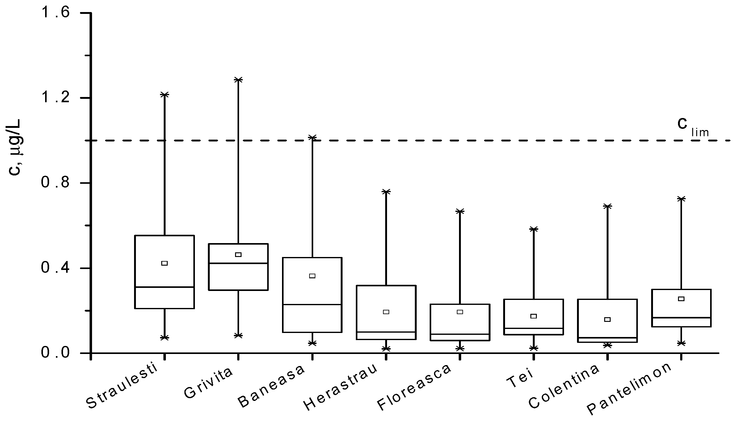
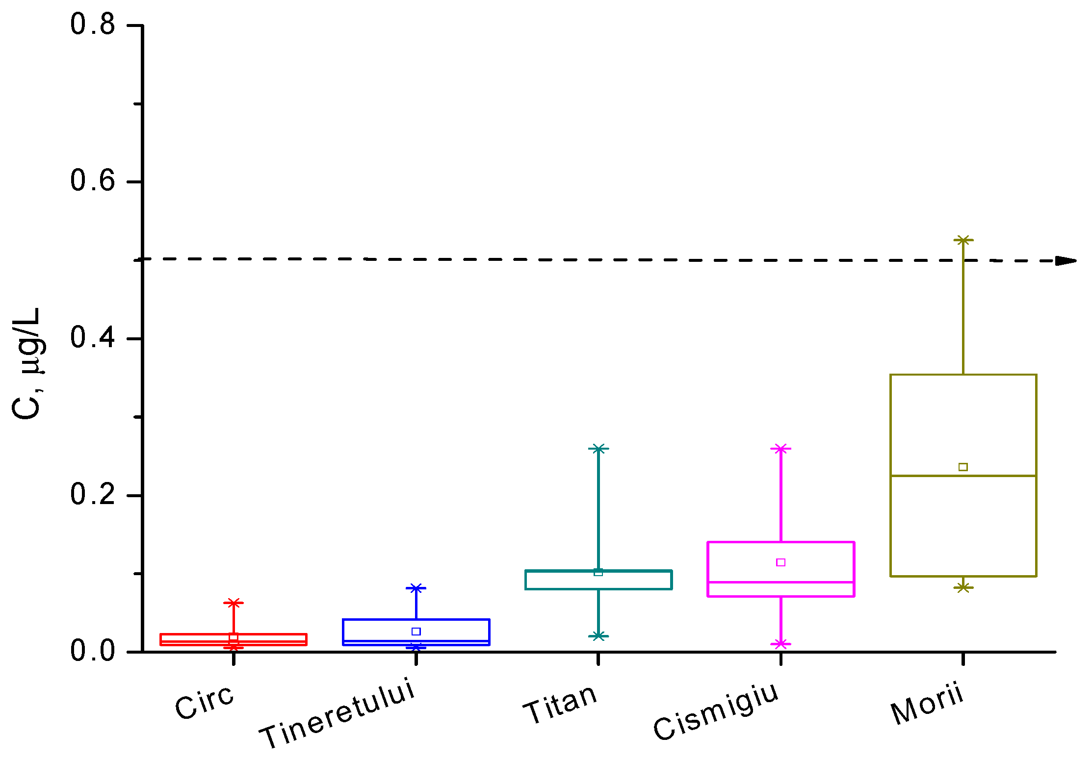
The maximum admitted limit of mercury is not attained in most of the surface waters around the Bucharest area, except the Morii, Griviţa, Străuleşti, and Băneasa Lakes, where this limit is accidentally overpassed.

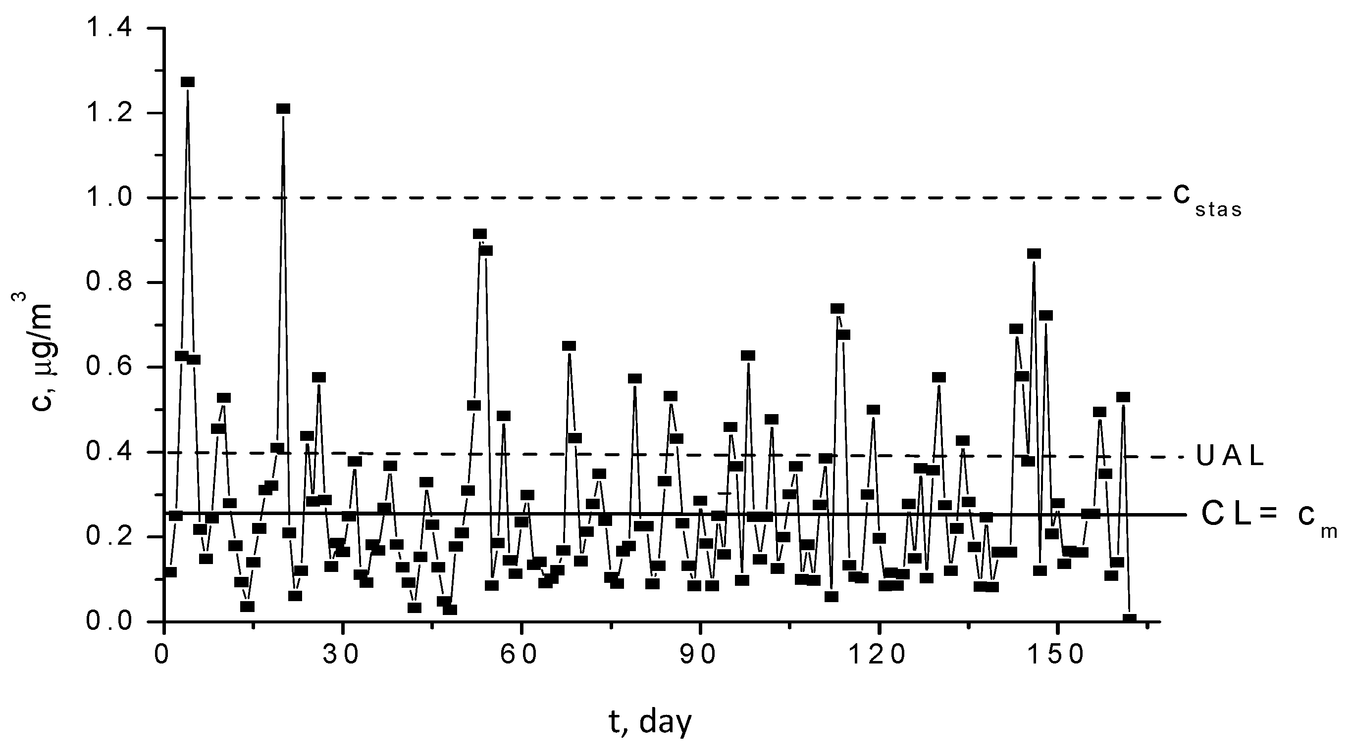
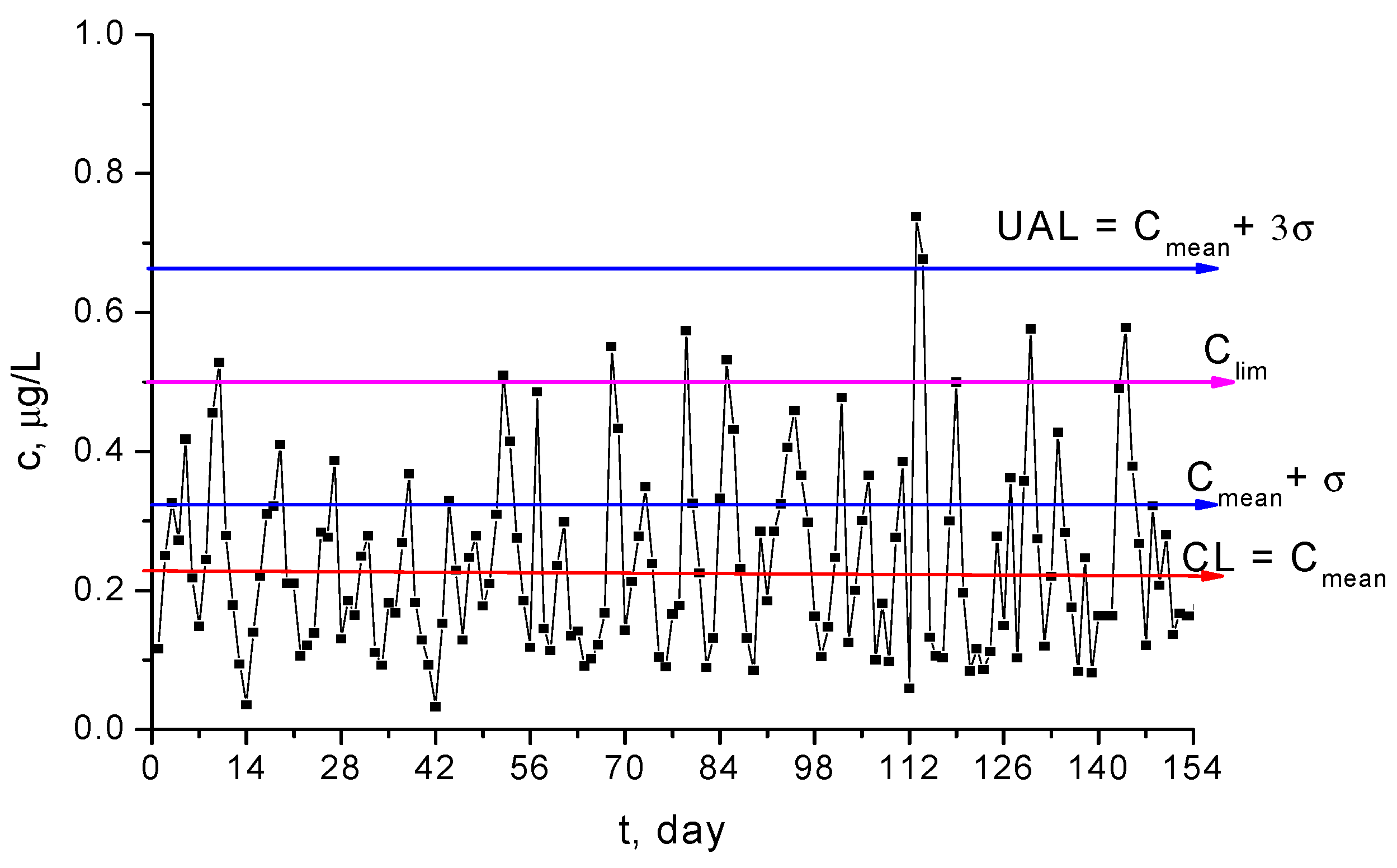
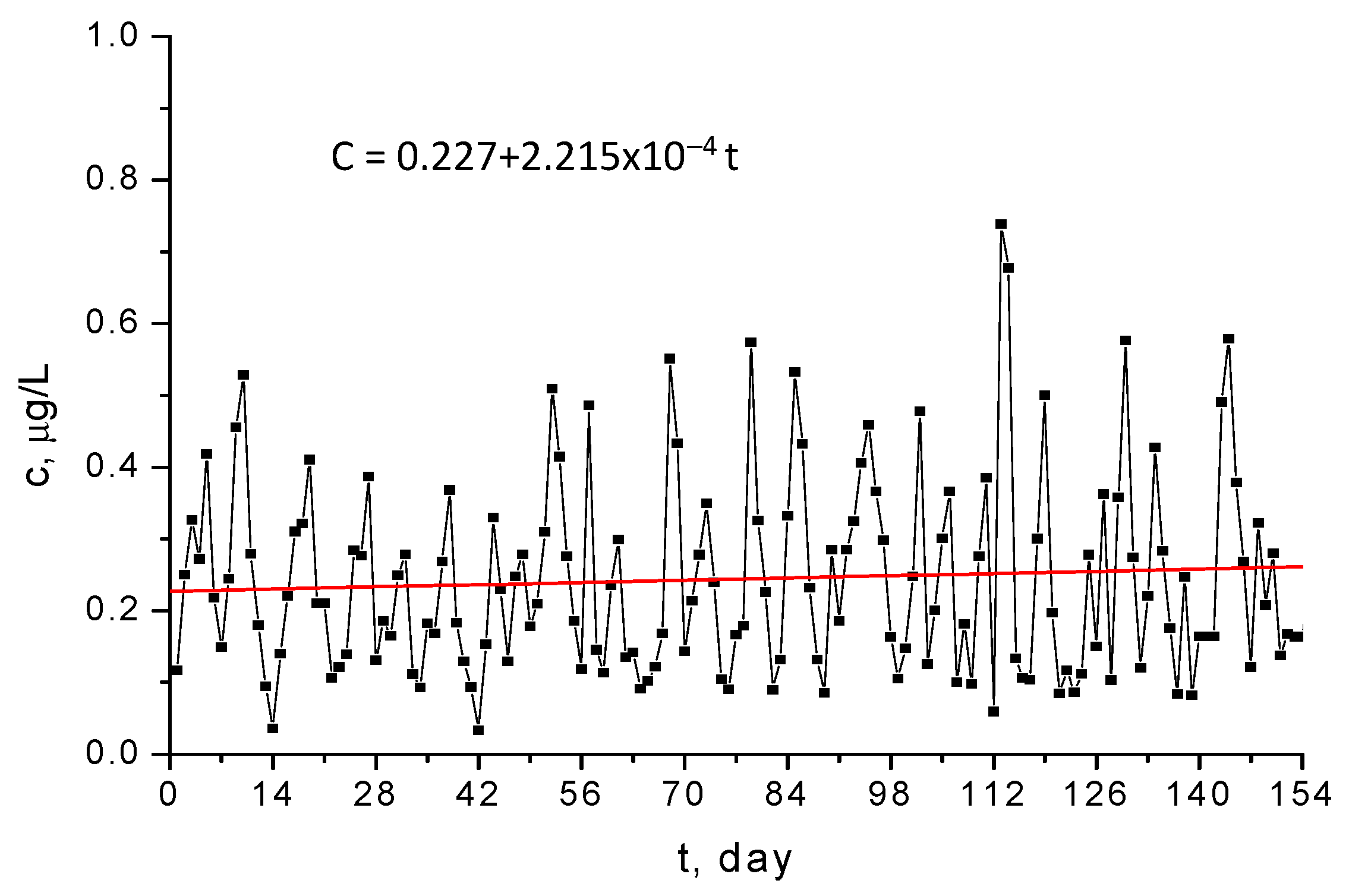
The monitored data on mercury concentration form a time series, which is not under statistic control since it is not stationary, having trend and periodicity. The distribution law is asymmetrical and the capability index, C_p, is less than 1.

Another time series based on concentration fluctuations was built, after the removal of trend and periodicity from the initial data, in order to obtain the statistical control. The novel time series is under statistical control because its distribution law is symmetrical and near the normal distribution, and, as a result, the 3σ rule is applied. The initial series of constitutive elements is recomposed, and then trend, periodicity, and fluctuations are changed to draw valuable conclusions on monitoring mercury concentrations in surface waters.

The highest mercury concentrations can be correlated with the intensity of road traffic, since the time variation is cyclic with a 7-day period, with smaller values during weekend and bigger values during the working days.

Eutrophication is the enrichment of water with nutrients. This process induces the growth of the biomass load and consequently may result in the depletion of oxygen in the water. The discharge of phosphate-containing fertilizers and sewage into aquatic systems is the main cause of eutrophication [57]. The phosphate-containing detergents were an important source of eutrophication and, since the end of the last century, gradually were replaced with environmentally-friendly detergents. The existence of phosphorus compounds causes a severe reduction of the quality of surface waters. Phosphorus is a necessary nutrient for plants and is the limiting factor for plant growth in many freshwater ecosystems. In agriculture, phosphate fertilizers adhere tightly to soil and so are transported by the erosion of lakes. The extraction of phosphate into water is slow, hence the difficulty of reversing the effects of eutrophication. Mainly due to the use of agricultural fertilizer, the rate of phosphorus cycling on Earth has increased by four times. As a result, the primary limiting factor for eutrophication is phosphate. In eutrophication management, the main component is the control of phosphorus sources.

The nutrients contained in organic matter are converted into inorganic forms by microorganisms in water systems when plants die. This process is oxygen-consuming, and it reduces the concentration of oxygen dissolved in water. The depleted oxygen levels lead to a range of effects reducing biodiversity. Nutrients can be concentrated in an anoxic zone and may only be made available again in conditions of turbulent flow, mainly generated by human activity. The enhanced growth of aquatic vegetation perturbs the normal functioning of the ecosystem, producing a variety of problems such as the lack of oxygen necessary for biotope survival. The value and aesthetic enjoyment of lakes decrease, since the water becomes muddy. The rate at which nutrients enter ecosystems can be accelerated by human activities. Although eutrophication is commonly caused by human activities, it can also be a natural process in lakes. Climate change is critical in regulating the natural productivity of nutrients in lakes. The main difference between natural and anthropogenic eutrophication is that the natural process is very slow, occurring on geological time scales.

Nitrogen is another typically limiting nutrient, because the chemical forms of this chemical element are related to eutrophication. The additions of nitrogen compounds stimulate the growth of plants since they have high nitrogen requirements. The ecosystems that receive more nitrogen than the plants require can contribute to water eutrophication. High levels of atmospheric compounds of nitrogen, mainly due to the traffic intensities, can increase nitrogen availability in surface waters.

Anyway, phosphorus fertilizers are generally much less soluble than nitrogen fertilizers. They are leached from the soil at a much slower rate than nitrogen. Therefore, phosphorus is much more important as a limiting nutrient in aquatic systems. The trophic state of lakes is related to phosphorus levels in water [58,59].

This article presents studies conducted between 2014 and 2016, regarding the eutrophication possibility of some lakes around Bucharest. The results prove that if current environmental conditions are maintained, there is no danger of eutrophication of these lakes. The obtained experimental data form a stationary time series with a uniform pattern. Two forecast methods have been applied that have yielded satisfactory results.

5. Conclusions

The aim of this paper is to highlight, compare, and discuss specific statistical methods and mathematical models to draw conclusions and to understand the causes and effects of surface waters pollution with heavy metals and the precursors of eutrophication. The methods and models are used to solve the concrete problems of three case studies, and they can be generalized and adapted for other similar problems.

This paper highlights some of the time series techniques for modeling and analysis of the daily heavy metal monitoring data measured in some important lakes around Bucharest between the months of March and November during the period 2007–2009. The daily registration of lead and mercury concentrations in surface waters form a univariate time series that consists of single scalar observations has been recorded sequentially over equal time intervals. This time series display periodicity that represents sinusoidal fluctuations over entire week and seasonality over the year. The seasonal pattern was consistent with a wave sine model. The highest mercury concentrations can be correlated with the intensity of road traffic, which is added to other existing sources.

In this work are also presented and analyzed data resulting from the monitoring of ions concentration for NO₂⁻, NO₃⁻ and PO₄³⁻ in surface waters from Bucharest during the 2013–2016 period. The statistical analysis of monitoring concentrations of these ions showed that they form a time series. The main properties of these time series have been determined. Time series data show the linear trend and seasonality for all these lakes. A method for modeling the time series was proposed to forecast the evolution of the pollution of those surface waters based on the obtained data.

Another direction of data analysis aims to establish whether there is a significant statistical difference between the concentrations of these pollutants in the surface waters analyzed. In this regard, the t test for two samples, assuming equal variances has been performed using Excel, and the results highlight that the pollution degrees of the lakes are similar, except for water surfaces from the beginning and the end of the lake chain. For these lakes, in addition to the mentioned sources, agricultural activity also contributes to their pollution.

6. Future Prospects

Mathematical methods, models, and statistical instruments used in pollution monitoring represent an important current scientific concern for the author, and the present paper is a step towards new research in water pollution evaluation.

Such statistical methods will be a starting point in the simulation and modeling of processes involving the use of microemulsions for the removal of pharmaceutical pollutants from water sources. Also, statistical instruments stay at the base of other research, where firstly a data base is needed.

It can be also emphasized that for the mine wastewater treatment, rare metals can be extracted, and there is no mathematical model devoted to simulating physical–chemical phenomena encountered in microemulsion processes, and particularly for those involved in the extraction and pre-concentration of heavy metals in order to be reused.

References

1. Wang, X.; Wang, G.; Tian, W.; Li, C.; Yang, Y. Characterizing Long-Term Water Quality Variation with Multivariate Statistical Methods: A Case Study in the Two Tributaries of Yellow River, China. Environ. Eng. Manag. J. 2022, 21, 1117–1125. [Google Scholar] [CrossRef]
2. Ismail, A.; Robescu, D. Application of Multivariate Statistical Techniques in Water Quality Assessment of Danube River, Romania. Environ. Eng. Manag. J. 2019, 18, 719–726. [Google Scholar] [CrossRef]
3. Sharma, V.; Sharma, M.; Pandita, S.; Kumar, V.; Kour, J.; Sharma, N. Assessment of water quality using different pollution indices and multivariate statistical techniques. In Heavy Metals in the Environment. Impact, Assessment, and Remediation; Elsevier: Amsterdam, The Netherlands, 2021; pp. 165–178. [Google Scholar]
4. Hue, N.H.; Thanh, N.H. Assessment of Surface Water Quality by Using Multivariate Statistical Analysis Techniques: A Case Study of Nhue River, Vietnam. Int. J. Environ. Sci. Dev. 2020, 11, 488–492. [Google Scholar] [CrossRef]
5. Da Silva, D.F.M.; Silva, L.M.L.; Gamier, J.; Araújo, D.F.; da Silva, L.A.; Mulholland, D.S. Linking Multivariate Statistical Methods and Water Quality Indices to Evaluate the Natural and Anthropogenic Geochemical Processes Controlling the Water Quality of a Tropical Watershed. Environ. Monit. Assess. 2023, 195, 1240. [Google Scholar] [CrossRef] [PubMed]
6. Dawood, A.S.; Faroon, M.A.; Yousif, Y.T. The use of multivariate statistical techniques in the assessment of river water quality. Anbar J. Eng. Sci. 2020, 11, 102–112. [Google Scholar] [CrossRef]
7. Abed, S.A.; Ewaid, S.H.; Al-Ansari, N. Evaluation of Water quality in the Tigris River within Baghdad, Iraq using Multivariate Statistical Techniques. J. Phys. Conf. Ser. 2019, 1294, 072025. [Google Scholar] [CrossRef]
8. Wang, Y.; Zhu, G.; Yu, R. Assessment of Surface Water Quality using Multivariate Statistical Techniques: A Case Study in China. Irrig. Drain. Syst. Eng. 2018, 7, 1000214. [Google Scholar]
9. Nguyen, H.Q.; Vuong, Q.P.; Pham-Thi, N.A.; Tran-Thi, T.T.; Ho, T.P.; Lam, S.H.T. Assessment of Surface Water Quality Using Multivariate Statistical Techniques: A Case Study of Saigon River. ChemRxiv 2020. [Google Scholar] [CrossRef]
10. Wang, Z.; Jia, D.; Song, S.; Sun, J. Assessments of surface water quality through the use of multivariate statistical techniques: A case study for the watershed of the Yuqiao Reservoir, China. Front. Environ. Sci. 2023, 11, 1107591. [Google Scholar] [CrossRef]
11. Liu, J.; Zhang, D.; Tang, Q.; Xu, H.; Huang, S.; Shang, D.; Liu, R. Water quality assessment and source identification of the Shuangji River (China) using multivariate statistical methods. PLoS ONE 2021, 16, e0245525. [Google Scholar] [CrossRef] [PubMed]
12. Özdemir, Ö. Application of Multivariate Statistical Methods for Water Quality Assessment of Karasu-Sarmisakli Creeks and Kizilirmak River in Kayseri, Turkey. Pol. J. Environ. Stud. 2016, 25, 1149–1160. [Google Scholar] [CrossRef]
13. Ma, X.; Wang, L.; Yang, H.; Li, N.; Gong, C. Spatiotemporal Analysis of Water Quality Using Multivariate Statistical Techniques and the Water Quality Identification Index for the Qinhuai River Basin, East China. Water 2020, 12, 2764. [Google Scholar] [CrossRef]
14. Gyimah, R.A.A.; Gyamfi, C.; Anornu, G.K.; Karikari, A.Y.; Tsyawo, F.W. Multivariate statistical analysis of water quality of the Densu River, Ghana. Int. J. River Basin Manag. 2020, 19, 189–199. [Google Scholar] [CrossRef]
15. Dawood, A.S.; Jabbar, M.T.; Al-Temeemi, H.H.; Baer, E.M. Application of Water Quality Index and Multivariate Statistical Techniques to Assess and Predict of Groundwater Quality with Aid of Geographic Information System. J. Ecol. Eng. 2022, 23, 189–204. [Google Scholar] [CrossRef]
16. Koklu, R.; Sengorur, B.; Topal, B. Water Quality Assessment Using Multivariate Statistical Methods—A Case Study: Melen River System (Turkey). Water Resour. Manag. 2010, 24, 959–978. [Google Scholar] [CrossRef]
17. Leventeli, Y.; Yalcin, F. Data analysis of heavy metal content in riverwater: Multivariate statistical analysis and inequality expressions. J. Inequalities Appl. 2021, 2021, 14. [Google Scholar] [CrossRef]
18. Gholikandi, G.B.; Orumieh, H.R.; Haddadi, S.; Mojir, N. Application of multivariate statistical techniques for surface water quality assessment: Case study of Karaj River, Iran. Water Resour. Manag. VI 2011, 145, 361–370. [Google Scholar]
19. Mohammed, A.; Samara, F.; Alzaatreh, A.; Knuteson, S.L. Statistical Analysis for Water Quality Assessment: A Case Study of Al Wasit Nature Reserve. Water 2022, 14, 3121. [Google Scholar] [CrossRef]
20. Bărbulescu, A.; Dumitriu, C.Ş. Assessing Water Quality by Statistical Methods. Water 2021, 13, 1026. [Google Scholar] [CrossRef]
21. Schreiber, S.G.; Schreiber, S.; Tanna, R.N.; Roberts, D.R.; Arciszewski, T.J. Statistical tools for water quality assessment and monitoring in river ecosystems—A scoping review and recommendations for data analysis. Water Qual. Res. 2022, 57, 40. [Google Scholar] [CrossRef]
22. Kovrov, O.; Kulikova, D.; Pavlychenko, A. Statistical analysis of Samara River pollution impact on the population morbidity rate in Western Donbas (Ukraine). IOP Conf. Ser. Earth Environ. Sci. 1156, 2023, 012025. [Google Scholar] [CrossRef]
23. Antonopoulos, V.Z.; Papamichail, D.M.; Mitsiou, K.A. Statistical and trend analysis of water quality and quantity data for the Strymon River in Greece. Hydrol. Earth Syst. Sci. 2001, 5, 679–691. [Google Scholar] [CrossRef]
24. Majerek, D.; Duda, S.; Babko, R.; Widomski, M.K. Statistical analysis of the water pollution indicators pertaining to treated municipal sewage introduced to the river. In Proceedings of the MATEC Web of Conferences 2019, Sibiu, Romania, 5–7 June 2019; Volume 252, p. 09009. [Google Scholar]
25. Stričević, L.; Pavlović, M.; Filipović, I.; Radivojević, A.; Bursać, N.M.; Gocić, M. Statistical analysis of water quality parameters in the basin of the Nišava River (Serbia) in the period 2009–2018. Geografie 2021, 126, 55–73. [Google Scholar] [CrossRef]
26. Khouri, L.; Al-Muft, M.B. Assessment of surface water quality using statistical analysis methods: Orontes River (Case study). Baghdad Sci. J. 2022, 19, 981–989. [Google Scholar] [CrossRef]
27. Bhat, S.A.; Meraj, G.; Yaseen, S.; Pandit, A.K. Statistical Assessment of Water Quality Parameters for Pollution Source Identification in Sukhnag Stream: An Inflow Stream of Lake Wular (Ramsar Site), Kashmir Himalaya. J. Ecosyst. 2014, 2014, 898054. [Google Scholar] [CrossRef]
28. Le, R.K.; Rackauckas, C.V.; Ross, A.S.; Ulloa, N. Assessment of Statistical Methods for Water Quality Monitoring in Maryland’s Tidal Waterways REU Site: Interdisciplinary Program in High Performance Computing. 2012. Available online: www.umbc.edu/hpcreu (accessed on 3 September 2023).
29. Andrejiová, M.; Kimáková, Z.; Knežo, D. Analysis of Water Pollution Indicators with the Use of Selected Statistical Methods. Acta Mech. Slovaca 2011, 15, 52–61. [Google Scholar] [CrossRef]
30. Wang, H.; Wang, S.; Wen, J.; Wang, S.; Zhu, M. Monitoring and statistical methods of irrigation water consumption of Wanyao Irrigation Area. IOP Conf. Ser. Earth Environ. Sci. 2020, 510, 032025. [Google Scholar] [CrossRef]
31. Fu, L.; Wang, Y.G. Statistical Tools for Analyzing Water Quality Data. In Water Quality Monitoring and Assessment; Voudouris, K., Voutsa, D., Eds.; IntechOpen: London, UK, 2012; pp. 143–168. [Google Scholar]
32. Helsel, D.R.; Hirsch, R.M. Statistical Methods in Water Resources. In Techniques of Water-Resources Investigations of the United States Geological Survey; Book 4, Hydrologic Analysis and Interpretation, USGS Science for A Changing World, Chapter A3; Elsevier: Amsterdam, The Netherlands, 2002. [Google Scholar]
33. Bal, K.J. Statistical Analysis for the Quality of Water. Master’s Thesis, Johannes Kepler University, Linz, Austria, 2023. [Google Scholar]
34. Hajigholizadeh, M. Water Quality Modelling Using Multivariate Statistical Analysis and Remote Sensing in South Florida. Ph.D. Thesis, Florida International University, Miami, FL, USA, 2016. [Google Scholar]
35. Meghea, I.; Mihai, M.; Lăcătuşu, I.; Iosub, I. Evaluation of Monitoring of Lead Emissions in Bucharest by Statistical Processing. J. Environ. Prot. Ecol. 2012, 13, 746–755. [Google Scholar]
36. Meghea, I.; Mihai, M.; Lăcătuşu, I.; Apostol, T. Time Series Model Applied to Environmental Monitoring Data Analyses. J. Environ. Prot. Ecol. 2012, 13, 426–434. [Google Scholar]
37. Meghea, I.; Mihai, M.; Lăcătuşu, I.; Apostol, T. Environmental monitoring of CO emissions: Statistical character of acquired data. Environ. Eng. Manag. J. 2009, 8, 575–582. [Google Scholar] [CrossRef]
38. Meghea, I.; Mihai, M. Statistical analysis of air monitoring data in Bucharest. In Proceedings of the 16th International Scientific GeoConference SGEM 2016, Albena Resort, Bulgaria, 28 June–7 July 2016; Book 4, Volume II, Energy and Clean Technologies. pp. 727–734. [Google Scholar]
39. Meghea, I.; Mihai, M. Air pollution with SO2 in Bucharest area. In Proceedings of the 15th International Scientific GeoConference SGEM 2015, Albena Resort, Bulgaria, 16–25 June 2015; Book 4, Vol. II, Air Pollution and Climate Change. pp. 1081–1088. [Google Scholar]
40. Meghea, I.; Mihai, M.; Demeter, T. Gauss dispersion model applied to multiple punctual sources from an industrial platform. In Proceedings of the 13th International Scientific GeoConference SGEM 2013, Albena Resort, Bulgaria, 16–22 June 2013; Volume I, pp. 497–504. [Google Scholar]
41. Mihai, M.; Meghea, I. Box Jenkins methodology applied to the evaluation of air quality in Bucharest. In Proceedings of the International Multidisciplinary 12th Scientific Geo Conference, SGEM 2012, Conference Proceedings, Albena Resort, Bulgaria, 17–23 June 2012; Volume V, Ecology and Environmental Protection. Environmental Legislation. Multilateral Relations and Funding Opportunities. pp. 125–132. [Google Scholar]
42. Meghea, I.; Mihai, M.; Crăciun, E. Statistical Control of Mercury in Surface Water of Bucharest. J. Environ. Prot. Ecol. 2012, 13, 1243–1252. [Google Scholar]
43. Meghea, I.; Mihai, M. Statistical study on pollution of surface waters in Bucharest. In Proceedings of the 17th International Scientific GeoConference SGEM 2017, Varna city, Bulgaria, 27 June–6 July 2017; Ecology, Economics, Education and Legislation. Volume 17, pp. 843–850. [Google Scholar]
44. Meghea, I.; Mihai, M.; Crăciun, E. Monitoring and statistics of heavy metals daily data in surface water. In Proceedings of the 10th International Scientific Geo Conference SGEM 2010, Albena resort, Bulgaria, 20–25 June 2010; Volume II, pp. 677–684. [Google Scholar]
45. Lista Lacurilor din București—Wikipedia. Available online: https://ro.wikipedia.org/wiki/Lista_lacurilor_din_Bucure%C8%99ti (accessed on 3 September 2023).
46. Anuarul Statistic al României. Available online: https://insse.ro/cms/sites/default/files/field/publicatii/anuarul_statistic_al_romaniei_carte-ed.2022.pdf (accessed on 3 September 2023).
47. Harrison, R.M. Pollution: Causes, Effects and Control, 4th ed.; The University of Birmingham: Birmingham, UK; The Royal Society of Chemistry: London, UK, 2001; pp. 51+67–68+354–355+513–515. [Google Scholar]
48. Salvato, J.A.; Nemerow, N.L.; Agardy, F.J. Environmental Engineering, 5th ed.; John Wiley & Sons: Hoboken, NJ, USA, 2003; pp. 116–119. [Google Scholar]
49. NABEL—La Pollution de l’air en 2010. OFEV, Berne 2011, Métaux Lourds dans les Poussières en Suspension et les Retombées de Poussières. pp. 65–70. Available online: https://www.bafu.admin.ch/dam/bafu/fr/dokumente/luft/uz-umwelt-zustand/nabel_luftbelastung2010.pdf.download.pdf/nabel_la_pollutiondelairen2010.pdf (accessed on 3 September 2023).
50. Lengyel, Z.; Lukacs, A.; Szabo, A.; Nagymajtenyi, L. General toxicity and neurotoxicity of lead and mercury in combination with dimethoate in rats after subchronic oral exposure. Trace Elem. Electrolytes 2006, 23, 242–246. [Google Scholar] [CrossRef]
51. Montgomery, D.C.; Runger, G. Applied Statistics and Probability for Engineers, 3rd ed.; John Wiley & Sons Inc.: Hoboken, NJ, USA, 2003. [Google Scholar]
52. Ryan, T. Modern Engineering Statistics; John Wiley & Sons Inc.: Hoboken, NJ, USA, 2007. [Google Scholar]
53. Walpole, R.; Myers, S.; Ye, K. Probability and Statistics for Engineers and Scientists; Pearson Prentice Hall: Hoboken, NJ, USA, 2007. [Google Scholar]
54. Marques de Sá, J. Applied Statistics Using SPSS, STATISTICA, MATLAB and R; Springer: Berlin/Heidelberg, Germany, 2007. [Google Scholar]
55. Williams, G. Mercury Pollution Prevention in Healthcare; National Wildlife Federation—Great Lakes Field Office: North Chicago, IL, USA, 1997. [Google Scholar]
56. Available online: http://people.uwec.edu/piercech/Hg/Pictures/merccycle.jpg (accessed on 3 September 2023).
57. Huang, J.; Xu, C.-C.; Ridoutt, B.G.; Wang, X.-C.; Rea, P.-A. Nitrogen and phosphorus losses and eutrophication potential associated with fertilizer application to cropland in China. J. Clean. Prod. 2017, 159, 171–179. [Google Scholar] [CrossRef]
58. Zhang, W.; Jin, X.; Liu, D.; Lang, C.; Shan, B. Temporal and spatial variation of nitrogen and phosphorus and eutrophication assessment for a typical arid river—Fuyang River in northern China. J. Environ. Sci. 2017, 55, 41–48. [Google Scholar] [CrossRef] [PubMed]
59. Yang, L.-K.; Peng, S.; Zhao, X.-H.; Li, X. Development of a two-dimensional eutrophication model in an urban lake (China) and the application of uncertainty analysis. Ecol. Model. 2017, 345, 63–74. [Google Scholar]
Figure 1. Location of lakes under monitoring, on Bucharest map (the numbers represent the six districts of Bucharest) [45].
Water 15 04178 g001
Figure 2. The ten lakes monitored—the result of the Colentina River systematizing [45].
Water 15 04178 g002
Figure 3. Box diagram for Pb2+ concentration in the lakes supplying Colentina River during March 2007–November 2009 period.
Water 15 04178 g003
Figure 4. Box diagram for Pb2+ concentration in lakes of the parks and Morii Lake during March 2007–November 2009 period.
Water 15 04178 g004
Figure 5. Shewhart diagram for Pb2+ concentration in Griviţa Lake during the period March–July 2009.
Water 15 04178 g005
Figure 6. CUSUM diagram for Pb2+ concentration in Griviţa Lake during the period March–July 2009.
Water 15 04178 g006
Figure 7. Trend of Pb2+ concentration in Griviţa Lake during March–July 2009 period.
Water 15 04178 g007
Figure 8. Weekly periodic character of Pb2+ concentration in Morii Lake during the period April–May 2009.
Water 15 04178 g008
Figure 9. Box diagram for the concentration of mercury ions in the lakes supplying the Colentina River during the period March 2007–November 2009.
Water 15 04178 g009
Figure 10. Box diagram for mercury ions concentration in the lakes of the parks and the Morii Lake during the period March 2007–November 2009.
Water 15 04178 g010
Figure 11. The Shewhart diagram for Hg2+ concentration in the Griviţa Lake during the period March–July 2009.
Water 15 04178 g011
Figure 12. Trend of the concentration of ions of mercury in the Griviţa Lake during the period March–July 2009.
Water 15 04178 g012
Figure 13. Weekly cyclicity of Hg2+ concentration in the Griviţa Lake during the period March–July 2009.
Water 15 04178 g013
Figure 14. Box diagram for fluctuations of Hg2+ concentration in the Floreasca Lake during the period March–May 2009.
Water 15 04178 g014
Figure 15. X diagram for concentration fluctuations presented in Figure 11.
Water 15 04178 g015
Figure 16. Range diagram R for diagram presented in Figure 14.
Water 15 04178 g016
Figure 17. Monthly concentrations of PO43− and Ptot, in the monitored lakes.
Water 15 04178 g017
Figure 18. Monthly concentrations of NO3− and NO2− in the monitored lakes.
Water 15 04178 g018
Figure 19. The time series of monthly mean concentration of PO43− and Ptot in the surface waters analyzed.
Water 15 04178 g019
Figure 20. Shewhart diagram for concentration fluctuations presented in Figure 5.
Water 15 04178 g020
Figure 21. Range diagram (R) for fluctuations of concentrations displayed in Figure 5.
Water 15 04178 g021
Figure 22. Annual mercury amounts deposited during the last two centuries [55].
Water 15 04178 g022
Figure 23. Mercury cycle in environment [56].
Water 15 04178 g023
Figure 24. Accumulation of mercury in food chain (EPA source) [55].
Water 15 04178 g024
Figure 25. Major sources of mercury in environment [55].
Water 15 04178 g025