


Data-Driven Models for Evaluating Coastal Eutrophication: A Case Study for Cyprus

 , , ,
, , ,  and
and 
Abstract
:1. Introduction
2. Materials and Methods
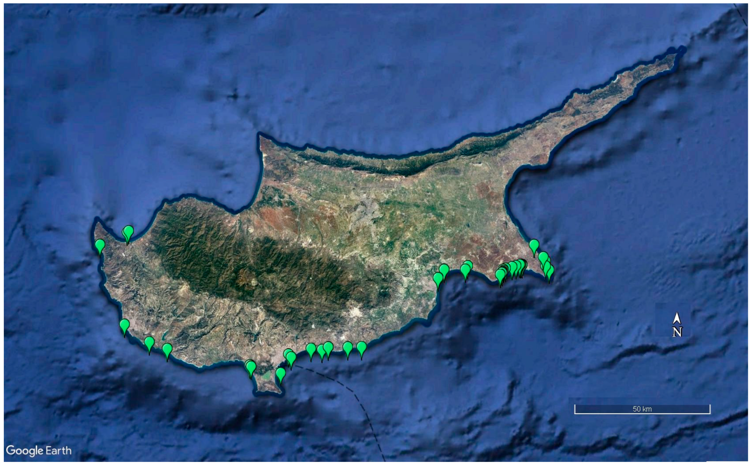
2.1. Study Area and Data Acquisition
2.2. Multilayer Feed-Forward ANNs
2.3. Self-Organizing Map (SOM)
- Initialize the weight vector with random values.
- Utilize a distance measure (e.g., the Euclidean distance) to calculate the best-matching unit (BMU).
- Move closer to the input vector by updating the weight vector of the BMU and the neighboring neurons.
3. Results
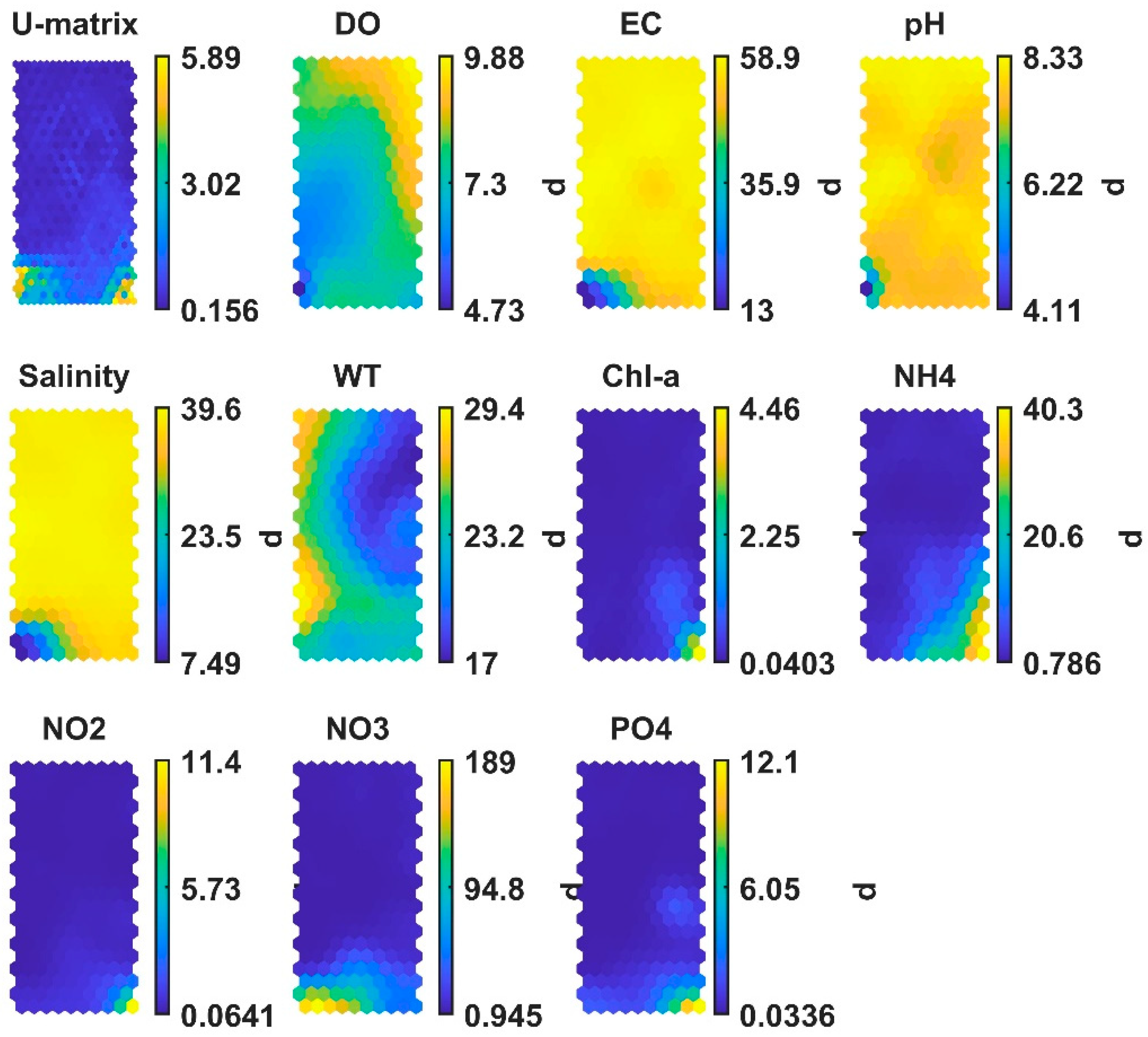
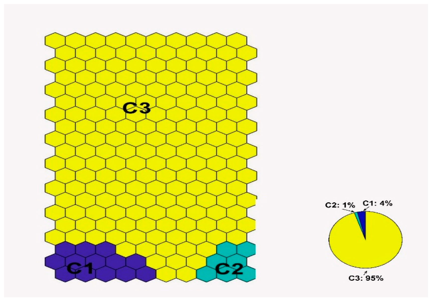
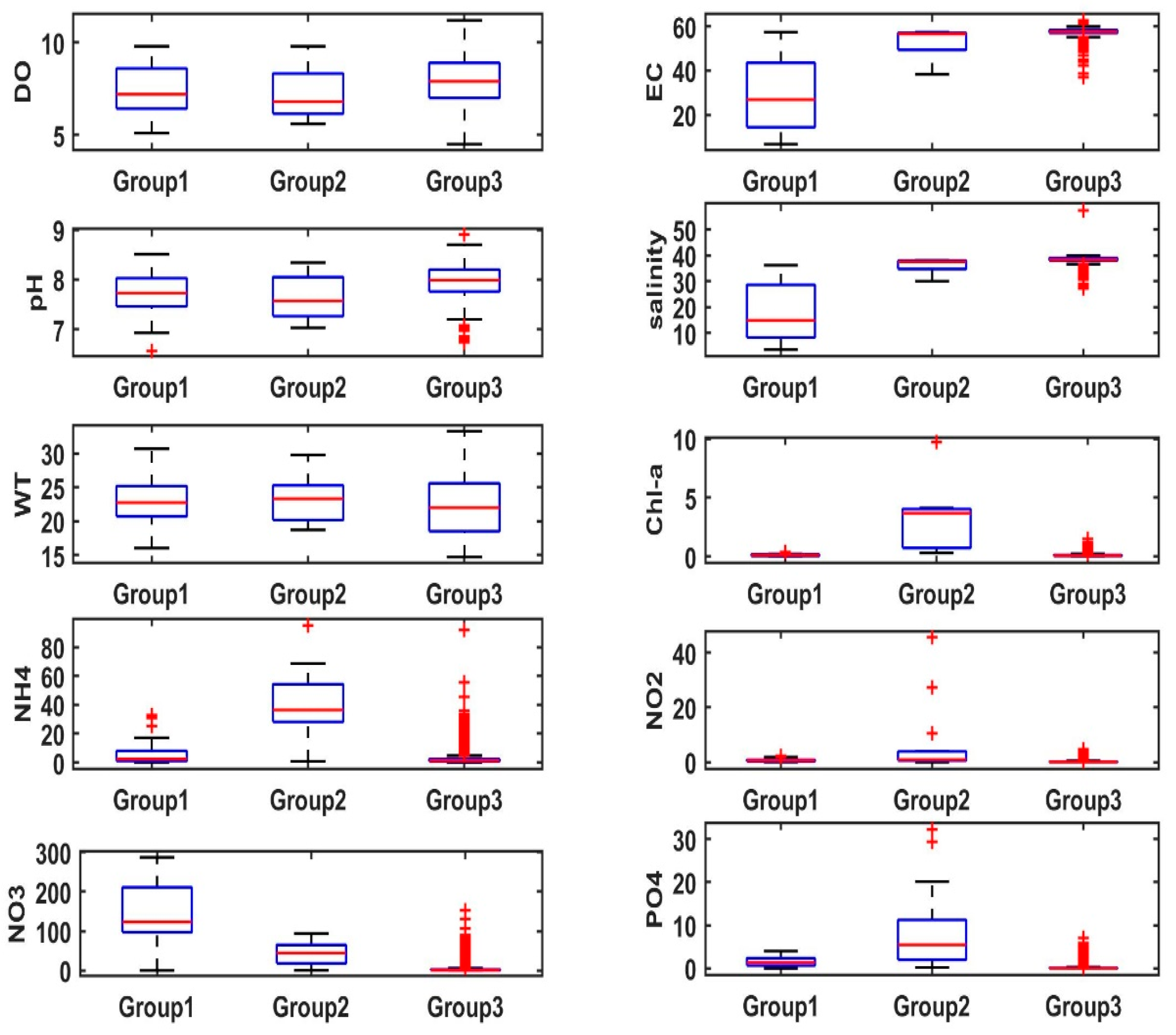
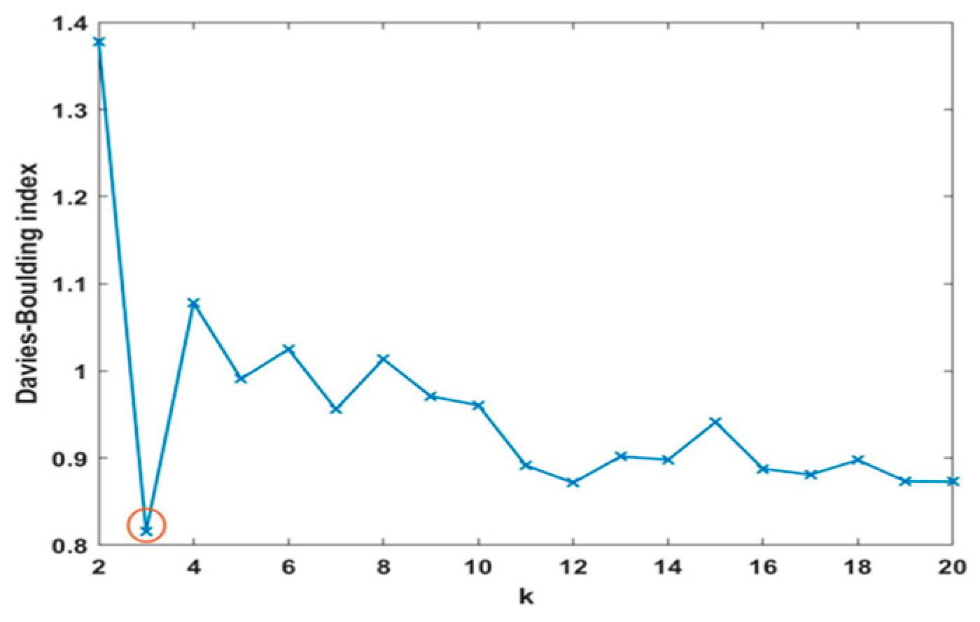
3.1. SOM’s Results
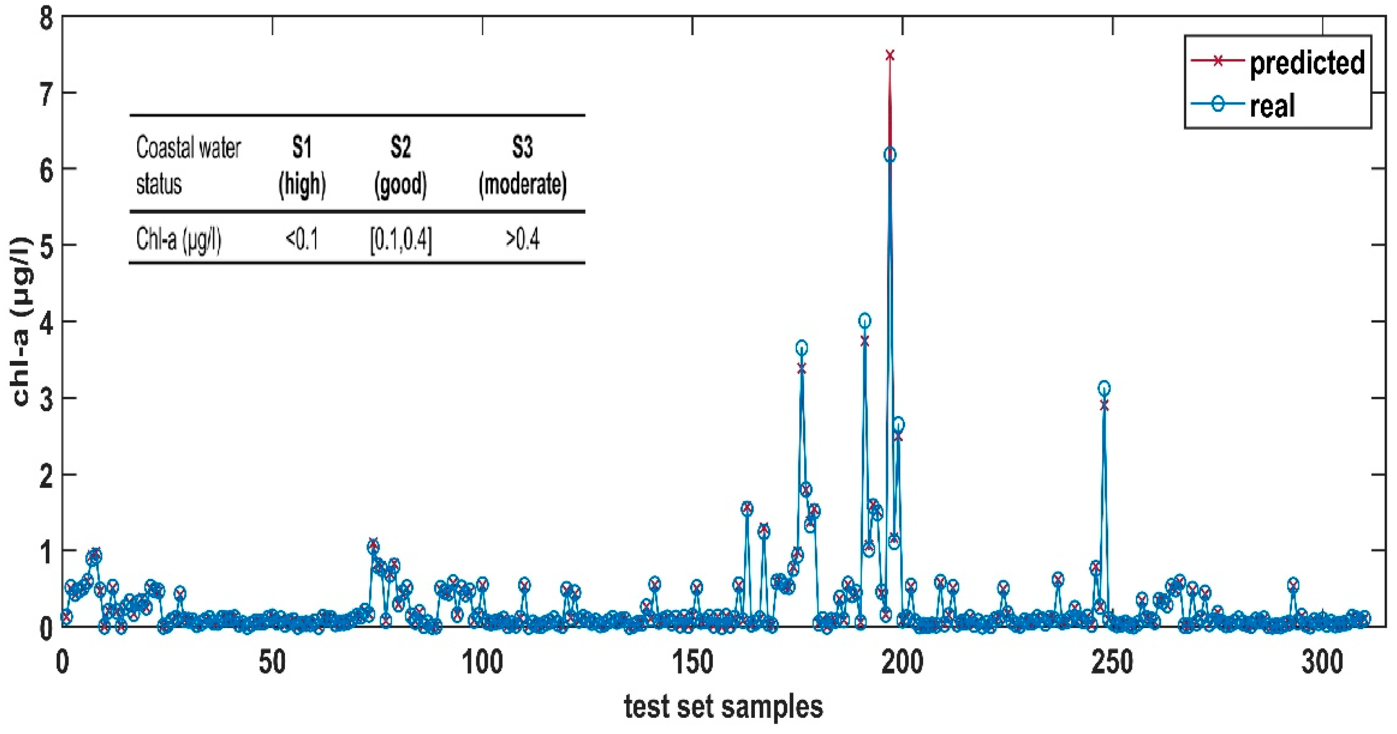
3.2. Feed-Forward ANN’s Results
4. Discussion
5. Conclusions
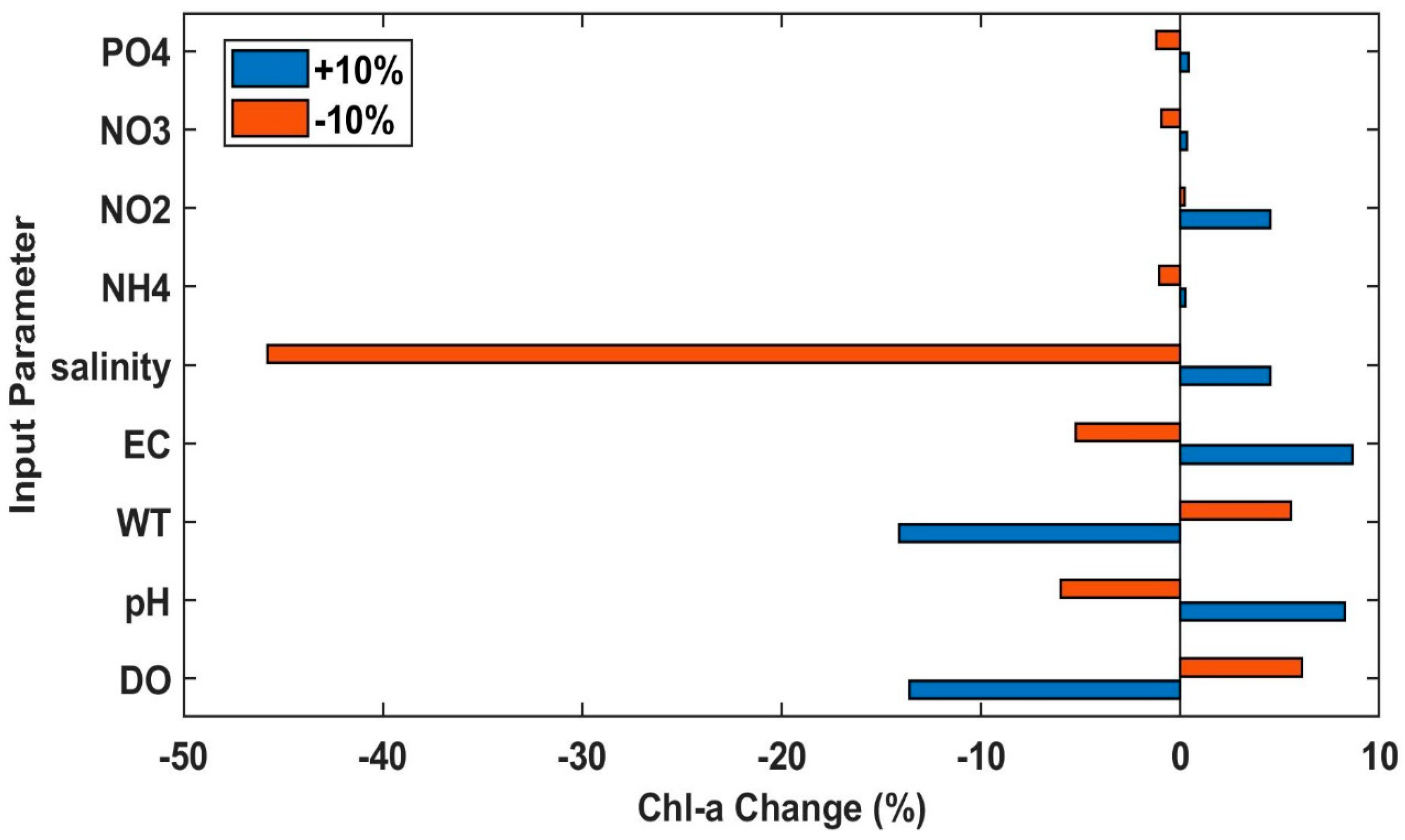
- The feed-forward ANN, based on the sensitivity analysis results, revealed that the winter upwelling seems to have an important role in the eutrophication phenomenon, while the cooler WT measurements are associated with higher Chl-a levels.
- Based on the SOM clustering results, the water quality of Cypriot coastal waters is classified as good and only few data samples (1.4%) are classified as not good.
Author Contributions
Funding
Data Availability Statement
Conflicts of Interest
References
- Visbeck, M. Ocean science research is key for a sustainable future. Nat. Commun. 2018, 9, 690. [Google Scholar] [CrossRef]
- Islam, S.; Tanaka, M. Impacts of pollution on coastal and marine ecosystems including coastal and marine fisheries and approach for management: A review and synthesis. Mar. Pollut. Bull. 2004, 48, 624–649. [Google Scholar] [CrossRef]
- Akiner, M.E. The problem of environmental pollution in the Mediterranean Sea along the coast of Turkey. J. Eng. Stud. Res. 2020, 26, 7–14. [Google Scholar] [CrossRef]
- He, Q.; Silliman, B.R. Climate Change, Human Impacts, and Coastal Ecosystems in the Anthropocene. Curr. Biol. 2019, 29, 1021–1035. [Google Scholar] [CrossRef] [PubMed]
- Alam, M.W.; Xiangmin, X.; Ahamed, R. Protecting the marine and coastal water from land-based sources of pollution in the northern Bay of Bengal: A legal analysis for implementing a national comprehensive act. Environ. Chall. 2021, 4, 100154. [Google Scholar] [CrossRef]
- Smith, V.H. Responses of estuarine and coastal marine phytoplankton to nitrogen and phosphorus enrichment. Limnol. Oceanogr. 2006, 51, 377–384. [Google Scholar] [CrossRef]
- Jiang, Z.B.; Liu, J.J.; Chen, J.F.; Chen, Q.Z.; Yan, X.J.; Xuan, J.L.; Zeng, J.N. Responses of summer phytoplankton community to drastic environmental changes in the Changjiang (Yangtze River) estuary during the past 50 years. Water Res. 2014, 54, 1–11. [Google Scholar] [CrossRef]
- Hadjisolomou, E.; Stefanidis, K.; Papatheodorou, G.; Papastergiadou, E. Assessing the Contribution of the Environmental Parameters to Eutrophication with the Use of the “PaD” and “PaD2” Methods in a Hypereutrophic Lake. Int. J. Environ. Res. Public Health 2016, 13, 764. [Google Scholar] [CrossRef]
- Kline, D.; Kuntz, N.; Breitbart, M.; Knowlton, N.; Rohwer, F. Role of Elevated Organic Carbon Levels and Microbial Activity in Coral Mortality. Mar. Ecol. Prog. Ser. 2006, 314, 119–125. [Google Scholar] [CrossRef]
- Tsikoti, C.; Genitsaris, S. Review of Harmful Algal Blooms in the Coastal Mediterranean Sea, with a Focus on Greek Waters. Diversity 2021, 13, 396. [Google Scholar] [CrossRef]
- Benkov, I.; Varbanov, M.; Venelinov, T.; Tsakovski, S. Principal Component Analysis and the Water Quality Index—A Powerful Tool for Surface Water Quality Assessment: A Case Study on Struma River Catchment, Bulgaria. Water 2023, 15, 1961. [Google Scholar] [CrossRef]
- Chau, K.-W. A review on integration of artificial intelligence into water quality modelling. Mar. Pollut. Bull. 2006, 52, 726–733. [Google Scholar] [CrossRef]
- Devillers, J. (Ed.) Artificial Neural Network Modeling of the Environmental Fate and Ecotoxicity of Chemicals. In Ecotoxicology Modeling; Springer: Boston, MA, USA, 2009. [Google Scholar]
- Youssef, K.; Shao, K.; Moon, S.; Bouchard, L.-S. Landslide susceptibility modeling by interpretable neural network. Commun. Earth Environ. 2023, 4, 162. [Google Scholar] [CrossRef]
- Kilic, H.; Soyupak, S.; Gurbuz, H.; Kivrak, E. Automata networks as preprocessing technique of artificial neural network in estimating primary production and dominating phytoplankton levels in a reservoir: An experimental work. Ecol. Inform. 2006, 1, 431–439. [Google Scholar] [CrossRef]
- Cereghino, R.; Park, Y.-S. Review of the Self-Organizing Map (SOM) approach in water resources: Commentary. Environ. Model. Softw. 2009, 24, 945–947. [Google Scholar] [CrossRef]
- Li, T.; Sun, G.; Yang, C.; Liang, K.; Ma, S.; Huang, L. Using self-organizing map for coastal water quality classification: Towards a better understanding of patterns and processes. Sci. Total Environ. 2018, 628–629, 1446–1459. [Google Scholar] [CrossRef] [PubMed]
- Peeters, L.; Dassargues, A. Comparison of Kohonen’s self-organizing map algorithm and principal component analysis in the exploratory data analysis of a groundwater quality dataset. In Proceedings of the 6th International Conference on Geostatistics for Environmental Applications, Rhodos, Greece, 25–27 October 2006; pp. 1–12. [Google Scholar]
- Park, Y.-S.; Verdonschot, P.F.M.; Chon, T.-S.; Lek, S. Patterning and predicting aquatic macroinvertebrate diversities using artificial neural network. Water Res. 2003, 37, 1749–1758. [Google Scholar] [CrossRef]
- Lu, R.S.; Lo, S.L. Diagnosing reservoir water quality using self-organizing maps and fuzzy theory. Water Res. 2002, 36, 2265–2274. [Google Scholar] [CrossRef] [PubMed]
- Li, J.; Shi, Z.; Wang, G.; Liu, F. Evaluating Spatiotemporal Variations of Groundwater Quality in Northeast Beijing by Self-Organizing Map. Water 2020, 12, 1382. [Google Scholar] [CrossRef]
- Hadjisolomou, E.; Antoniadis, K.; Vasiliades, L.; Rousou, M.; Thasitis, I.; Abualhaija, R.; Herodotou, H.; Michaelides, M.; Kyriakides, I. Predicting Coastal Dissolved Oxygen Values with the Use of Artificial Neural Networks: A Case Study for Cyprus. IOP Conf. Ser. Earth Environ. Sci. 2022, 1123, 012083. [Google Scholar] [CrossRef]
- Salami, E.S.; Salari, M.; Rastergarc, M.; Sheibani, S.N.; Ehteshami, M. Artificial neural network and mathematical approach for estimation of surface water quality parameters (case study: California, USA). Desalin. Water Treat. 2021, 213, 75–83. [Google Scholar] [CrossRef]
- Melesse, A.; Krishnaswamy, J.; Zhang, K. Modeling Coastal Eutrophication at Florida Bay using Neural Networks. J. Coast. Res. 2009, 24, 190–196. [Google Scholar] [CrossRef]
- Hadjisolomou, E.; Stefanidis, K.; Herodotou, H.; Michaelides, M.; Papatheodorou, G.; Papastergiadou, E. Modelling Freshwater Eutrophication with Limited Limnological Data Using Artificial Neural Networks. Water 2021, 13, 1590. [Google Scholar] [CrossRef]
- Georgescu, P.L.; Moldovanu, S.; Iticescu, C.; Calmuc, M.; Calmuc, V.; Topa, C.; Moraru, L. Assessing and forecasting water quality in the Danube River by using neural network approaches. Sci. Total Environ. 2023, 879, 162998. [Google Scholar] [CrossRef] [PubMed]
- Moiseenko, T.I. Surface Water under Growing Anthropogenic Loads: From Global Perspectives to Regional Implications. Water 2022, 14, 3730. [Google Scholar] [CrossRef]
- Tselepides, A.; Papadopoulou, N.; Podaras, D.; Plaiti, W.; Koutsoubas, D. Macrobenthic community structure over the continental margin of Crete (South Aegean Sea NE Mediterranean). Prog. Oceanogr. 2000, 46, 401–428. [Google Scholar] [CrossRef]
- Azov, Y. Eastern Mediterranean—A marine desert? Mar. Pollut. Bull. 1991, 23, 225–232. [Google Scholar] [CrossRef]
- Antoniadis, K.; Rousou, M.; Markou, M.; Stavrou, P.; Vasileiou, E.; Vasiliades, V.; Iosiphides, M.; Papadopoulos, V.; Argyrou, M. Review-Update Report of the Coastal Waters in Accordance with Article 5 of the Water Framework Directive (WFD) 2000/60/EC for the Period 2013–2019. Department of Fisheries and Marine Research, Ministry of Agriculture, Rural Development and the Environment, Cyprus. 2020. Available online: http://www.moa.gov.cy/moa/dfmr/ (accessed on 12 May 2022). (In Greek)
- Kuo, Y.-M.; Liu, C.-W.; Lin, K.-H. Evaluation of the ability of an artificial neural network model to assess the variation of groundwater quality in an area of blackfoot disease in Taiwan. Water Res. 2004, 38, 148–158. [Google Scholar] [CrossRef]
- Kohonen, T.; Kaski, S. Exploratory Data Analysis by The Self Organizing Maps: Structure of Welfare and Poverty in the World. In Proceedings of the Third International Conference on Neural Networks in the Capital Markets, London, UK, 11–13 October 1995. [Google Scholar]
- Dedecker, A.P.; Goethals, P.L.M.; Gabriels, W.; De Pauw, N. Optimization of Artificial Neural Network (ANN) model design for prediction of macroinvertebrates in the Zwalm river basin (Flanders, Belgium). Ecol. Model. 2004, 174, 161–173. [Google Scholar] [CrossRef]
- Hu, Z.; Zhang, Y.; Zhao, Y.; Xie, M.; Zhong, J.; Tu, Z.; Liu, J. A Water Quality Prediction Method Based on the Deep LSTM Network Considering Correlation in Smart Mariculture. Sensors 2019, 19, 1420. [Google Scholar] [CrossRef] [PubMed]
- Lee, J.H.W.; Huang, Y.; Dickman, M.; Jayawardena, A.W. Neural networking modelling of coastal algal blooms. Ecol. Model. 2003, 159, 179–201. [Google Scholar] [CrossRef]
- Kohonen, T. Self-Organising Maps; Springer: Berlin/Heidelberg, Germany, 2001. [Google Scholar]
- Al-Mudhaf, H.F.; Astel, A.M.; Selim, M.I.; Abu-Shady, A.I. Self-organizing map approach in assessment spatiotemporal variations of trihalomethanes in desalinated drinking water in Kuwait. Desalination 2010, 252, 97–105. [Google Scholar] [CrossRef]
- Park, Y.-S.; Tison, J.; Lek, S.; Giraudel, J.-L.; Coste, M.; Delmas, F. Application of a self-organizing map to select representative species in multivariate analysis: A case study determining diatom distribution patterns across France. Ecol. Inform. 2006, 1, 247–257. [Google Scholar] [CrossRef]
- An, Y.; Zou, Z.; Li, R. Descriptive Characteristics of Surface Water Quality in Hong Kong by a Self-Organising Map. Int. J. Environ. Res. Public Health 2016, 13, 115. [Google Scholar] [CrossRef]
- Choi, J.-Y.; Kim, S.-K.; Jeng, K.-S.; Joo, G.-J. Detecting response patterns of zooplankton to environmental parameters in shallow freshwater wetlands: Discovery of the role of macrophytes as microhabitat for epiphytic zooplankton. J. Ecol. Environ. 2015, 38, 133–143. [Google Scholar] [CrossRef]
- Kim, D.-K.; Kaluskar, S.; Mugalingam, S.; Arhonditsis, G.B. Evaluating the relationships between watershed physiography, land use patterns, and phosphorus loading in the bay of Quinte basin, Ontario, Canada. J. Great Lakes Res. 2016, 42, 972–984. [Google Scholar] [CrossRef]
- Vesanto, J.; Alhoniemi, E. Clustering of the Self-Organizing Map. IEEE Trans. Neural Netw. 2000, 11, 586–600. [Google Scholar] [CrossRef]
- Vesanto, J. SOM-based data visualization methods. Intell. Data Anal. 1999, 3, 111–126. [Google Scholar] [CrossRef]
- Kalteh, A.M.; Hjorth, P.; Berndtsson, R. Review of the Self-Organizing Map (SOM) approach in water resources: Analysis, modelling and application. Environ. Model. Softw. 2008, 23, 835–845. [Google Scholar] [CrossRef]
- Vesanto, J.; Alhoniemi, E.; Himberg, J.; Parhankangas, J. SOM Toolbox for Matlab. 2000. Available online: http://www.cis.hut.fi/projects/somtoolbox/ (accessed on 5 April 2023).
- Garcia-Avila, F.; Loja-Suco, P.; Siguenza-Jeton, C.; Jimenez-Ordonez, M.; Valdiviezo-Gonzales, L.; Cabello-Torres, R.; Aviles-Anazco, A. Evaluation of the water quality of a high Andean lake using different quantitative approaches. Ecol. Indic. 2023, 154, 110924. [Google Scholar] [CrossRef]
- Bernard, J.; Landesberger, T.; Bremm, S.; Schreck, T. Multi-Scale Visual Quality Assessment for Cluster Analysis with Self-Organizing Maps. In Proceedings of the SPIE Conference on Visualization and Data Analysis, San Francisco, CA, USA, 23–27 January 2011; SPIE: Bellingham, WA, USA, 2011; Volume 7868. [Google Scholar] [CrossRef]
- Wang, X.; Li, Y.; Qiao, Q.; Tavares, A.; Liang, Y. Water Quality Prediction Based on Machine Learning and Comprehensive Weighting Methods. Entropy 2023, 25, 1186. [Google Scholar] [CrossRef] [PubMed]
- Zhang, P.; Hong, B.; He, L.; Cheng, F.; Zhao, P.; Wei, C.; Liu, Y. Temporal and spatial simulation of atmospheric pollutant PM2.5 changes and risk assessment on population exposure to pollution using optimization algorithms of the back propagation-Artificial Neural Network model and GIS. Int. J. Environ. Res. Public Health 2015, 12, 12171–12195. [Google Scholar] [CrossRef]
- Chon, T.-S. Self-Organizing Maps applied to ecological sciences. Ecol. Inform. 2011, 6, 50–61. [Google Scholar] [CrossRef]
- Qian, J.; Nguyen, N.P.; Oya, Y.; Kikugawa, G.; Okabe, T.; Huang, Y.; Ohuchi, F.S. Introducing self-organized maps (SOM) as a visualization tool for materials research and education. Results Mater. 2019, 4, 100020. [Google Scholar] [CrossRef]
- Krasznai, E.; Boda, P.; Csercsa, A.; Ficsor, M.; Varbiro, G. Use of self-organizing maps in modelling the distribution patterns of gammarids (Crustacea: Amphipoda). Ecol. Inform. 2016, 31, 39–48. [Google Scholar] [CrossRef]
- Astel, A.; Tsakovski, S.; Barbieri, P.; Simeonov, V. Comparison of self-organizing maps classification approach with cluster and principal components analysis for large environmental data sets. Water Res. 2007, 41, 4566–4578. [Google Scholar] [CrossRef]
- Varbiro, G.; Acs, E.; Borics, G.; Erces, K.; Feher, G.; Grigorszky, I.; Japport, T.; Kocsis, G.; Krasznai, E.; Nagy, K.; et al. Use of Self-Organizing Maps (SOM) for characterization of riverine phytoplankton associations in Hungary. Arch. Hydrobiol. 2007, 17, 383–394. [Google Scholar]
- Palani, S.; Liong, S.-Y.; Tkalich, P. An ANN application for water quality forecasting. Mar. Pollut. Bullet. 2008, 56, 1586–1597. [Google Scholar] [CrossRef]
- Bushra, B.; Bazneh, L.; Deka, L.; Wood, P.J.; McGowan, S.; Das, D.B. Temporal modelling of long-term heavy metal concentrations in aquatic ecosystems. J. Hydroinformatics 2023, 25, 1188–1209. [Google Scholar] [CrossRef]
- Brown, M.G.L.; Skakun, S.; He, T.; Liang, S. Intercomparison of Machine-Learning Methods for Estimating Surface Shortwave and Photosynthetically Active Radiation. Remote Sens. 2020, 12, 372. [Google Scholar] [CrossRef]
- Petrou, A.; Kallianiotis, A.; Hannides, A.K.; Charalambidou, I.; Hadjichristoforou, M.; Hayes, D.R.; Lambridis, C.; Lambridi, V.; Loizidou, X.I.; Orfanidis, S.; et al. Initial Assessment of the Marine Environment of Cyprus: Part I—Characteristics; Ministry of Agriculture, Natural Resources, and the Environment, Department of Fisheries and Marine Research: Nicosia, Cyprus, 2012. [Google Scholar]
- Fyttis, G.; Zervoudaki, S.; Sakavara, A.; Sfenthourakis, S. Annual cycle of mesozooplankton at the coastal waters of Cyprus (Eastern Levantine basin). J. Plankton Res. 2023, 45, 291–311. [Google Scholar] [CrossRef] [PubMed]
- Espinosa-Carreon, T.; Gaxiola-Castro, G.; Robles-Pacheco, J.; Najera-Martínez, S. Temperature, salinity, nutrients and chlorophyll a in coastal waters of the Southern California Bight. Cienc. Mar. 2001, 27, 397–422. [Google Scholar] [CrossRef]
- Georgiou, N.; Fakiris, E.; Koutsikopoulos, C.; Papatheodorou, G.; Christodoulou, D.; Dimas, X.; Geraga, M.; Kapellonis, Z.G.; Vaziourakis, K.-M.; Noti, A.; et al. Spatio-Seasonal Hypoxia/Anoxia Dynamics and Sill Circulation Patterns Linked to Natural Ventilation Drivers, in a Mediterranean Landlocked Embayment: Amvrakikos Gulf, Greece. Geosciences 2021, 11, 241. [Google Scholar] [CrossRef]
- Suursaar, U. Winter upwelling in the Gulf of Finland, Baltic Sea. Oceanologia 2021, 63, 356–369. [Google Scholar] [CrossRef]
- Ren, L.; Huang, J.; Zhu, H.; Jiang, W.; Wu, H.; Pan, Y.; Mao, Y.; Luo, M.; Jeong, T. Effects of Algal Utilization of Dissolved Organic Phosphorus by Microcystis Aeruginosa on Its Adaptation Capability to Ambient Ultraviolet Radiation. J. Mar. Sci. Eng. 2022, 10, 1257. [Google Scholar] [CrossRef]
- Paerl, H.; Dennis, R.; Whitall, D. Atmospheric Deposition of Nitrogen: Implications for Nutrient Over-Enrichment of Coastal Waters. Estuaries Coast. 2002, 25, 677–693. [Google Scholar] [CrossRef]
- Droge, R.; Kroeze, C. Critical load exceedance for nitrogen in the Ebrié Lagoon (Ivory Coast): A first assessment. J. Integr. Environ. Sci. 2007, 4, 5–19. [Google Scholar] [CrossRef]
- Duarte, I.; Ribeiro, M.C.; Pereira, M.J.; Leite, P.P.; Peralta-Santos, A.; Azevedo, L. Spatiotemporal evolution of COVID-19 in Portugal’s Mainland with self-organizing maps. Int. J. Health Geogr. 2023, 22, 4. [Google Scholar] [CrossRef]
- Varbiro, G.; Borics, G.; Kiss, T.K.; Szabo, K.E.; Plenkovic-Moraj, A.; Acs, E. Use of Kohonen Self Organizing Maps (SOM) for the characterization of benthic diatom associations of the River Danube and its tributaries. Arch. Hydrobiol. 2007, 17, 395–403. [Google Scholar]
- Hadjisolomou, E.; Antoniades, K.; Thasitis, I.; Abu Alhaija, R.; Herodotou, H.; Michaelides, M. Exploring the Impact of Coastal Water Quality Parameters on Chlorophyll-a near Cyprus with the use of Artificial Neural Networks. In Proceedings of the IAHR World Congress, Granada, Spain, 19–24 June 2022. [Google Scholar] [CrossRef]
- Shah, M.I.; Alaloul, W.S.; Alqahtani, A.; Aldrees, A.; Musarat, M.A.; Javed, M.F. Predictive Modeling Approach for Surface Water Quality: Development and Comparison of Machine Learning Models. Sustainability 2021, 13, 7515. [Google Scholar] [CrossRef]
- Ahmed, A.A.M.; Jui, S.J.J.; Chowdhury, M.A.I.; Ahmed, O.; Sutradha, A. The development of dissolved oxygen forecast model using hybrid machine learning algorithm with hydro-meteorological variables. Env. Sci Pollut. Res. 2023, 30, 7851–7873. [Google Scholar] [CrossRef] [PubMed]
- Ahmed, A.A.M. Prediction of dissolved oxygen in Surma River by biochemical oxygen demand and chemical oxygen demand using the artificial neural networks (ANNs). J. King Saud Univ. Eng. Sci. 2017, 29, 151–158. [Google Scholar] [CrossRef]
- Kitsiou, D.; Karydis, M. Coastal marine eutrophication assessment: A review on data analysis. Environ. Int. 2011, 37, 778–801. [Google Scholar] [CrossRef] [PubMed]


| Variable | Units | Min. | Max. | Mean ± SD |
|---|---|---|---|---|
| Salinity | psu | 0.86 | 44.05 | 37.74 ± 2.88 |
| pH | - | 0.25 | 8.79 | 7.88 ± 0.48 |
| Dissolved Oxygen | mg/L | 1.6 | 8.61 | 7.84 ± 0.39 |
| Chlorophyll-a | μg/L | 0.01 | 10.80 | 0.22 ± 0.59 |
| Water Temperature | °C | 21.68 | 27.69 | 22.25 ± 0.32 |
| Electrical Conductivity | mS/cm | 0.8 | 67.15 | 56.34 ± 4.79 |
| Orthophosphates | µmol/L | 0.00 | 17.77 | 0.46 ± 0.98 |
| Ammonium | µmol/L | 0.99 | 65.39 | 4.03 ± 3.51 |
| Nitrite | µmol/L | 0.00 | 24.21 | 0.49 ± 1.31 |
| Nitrate | µmol/L | 0.01 | 448.74 | 11.74 ± 24.94 |
Disclaimer/Publisher’s Note: The statements, opinions and data contained in all publications are solely those of the individual author(s) and contributor(s) and not of MDPI and/or the editor(s). MDPI and/or the editor(s) disclaim responsibility for any injury to people or property resulting from any ideas, methods, instructions or products referred to in the content. |
© 2023 by the authors. Licensee MDPI, Basel, Switzerland. This article is an open access article distributed under the terms and conditions of the Creative Commons Attribution (CC BY) license (https://creativecommons.org/licenses/by/4.0/).
Share and Cite
Hadjisolomou, E.; Rousou, M.; Antoniadis, K.; Vasiliades, L.; Kyriakides, I.; Herodotou, H.; Michaelides, M. Data-Driven Models for Evaluating Coastal Eutrophication: A Case Study for Cyprus. Water 2023, 15, 4097. https://doi.org/10.3390/w15234097
Hadjisolomou E, Rousou M, Antoniadis K, Vasiliades L, Kyriakides I, Herodotou H, Michaelides M. Data-Driven Models for Evaluating Coastal Eutrophication: A Case Study for Cyprus. Water. 2023; 15(23):4097. https://doi.org/10.3390/w15234097
Chicago/Turabian StyleHadjisolomou, Ekaterini, Maria Rousou, Konstantinos Antoniadis, Lavrentios Vasiliades, Ioannis Kyriakides, Herodotos Herodotou, and Michalis Michaelides. 2023. "Data-Driven Models for Evaluating Coastal Eutrophication: A Case Study for Cyprus" Water 15, no. 23: 4097. https://doi.org/10.3390/w15234097
APA StyleHadjisolomou, E., Rousou, M., Antoniadis, K., Vasiliades, L., Kyriakides, I., Herodotou, H., & Michaelides, M. (2023). Data-Driven Models for Evaluating Coastal Eutrophication: A Case Study for Cyprus. Water, 15(23), 4097. https://doi.org/10.3390/w15234097