Article

Predicting the Presence of Groundwater-Influenced Ecosystems in the Northeastern United States with Ensembled Models

1
Department of Wildlife, Fisheries and Conservation Biology, University of Maine, 5755 Nutting Hall, Orono, ME 04469, USA
2
U.S. Geological Survey, Cooperative Research Units, Reston, VA 20192, USA
3
School of Earth and Climate Sciences, University of Maine, Orono, ME 04469, USA
*
Author to whom correspondence should be addressed.
Water 2023, 15(23), 4035; https://doi.org/10.3390/w15234035
Submission received: 25 September 2023 / Revised: 13 November 2023 / Accepted: 14 November 2023 / Published: 21 November 2023
(This article belongs to the Special Issue Ecohydrology: Insights into Water Dynamics and Ecosystem Functioning)

Abstract

:
Globally, groundwater-influenced ecosystems (GIEs) are increasingly vulnerable to groundwater extraction and land use practices. Groundwater supports these ecosystems by providing inflow, which can maintain water levels, water temperature, and the chemistry necessary to sustain the biodiversity that they support. Many aquatic systems receive groundwater as a portion of baseflow, and in some systems, the connection with groundwater is significant and important to the system’s integrity and persistence. There is a lack of information about where these systems are found and their relationships with environmental conditions in the surrounding landscape. Additionally, groundwater management for human use often does not address maintaining the ecological functions of GIEs. We used correlative distribution modeling methods (GLM, GAM, MaxEnt, Random Forest) to predict landscape-scale habitat suitability for GIEs in two ecologically distinct ecoregions (EPA Level II ecoregions: Atlantic Highlands and Mixed Wood Plains) in the northeastern United States. We evaluated and combined the predictions to create ensemble models for each ecoregion. The accuracy of the ensemble models was 75% in the Atlantic Highlands and 86% in the Mixed Wood Plains. In the Mixed Wood Plains, hydric soil, surface materials, and soil permeability were the best predictors of GIE presence, whereas hydric soil, topographic wetness index, and elevation were the best predictors of GIE presence in the Atlantic Highlands. Approximately 1% of the total land area in each ecoregion was predicted to be suitable for GIEs, highlighting that there likely is a small proportion of the landscape occupied by these systems.

1. Introduction

Many surface water systems (i.e., rivers, lakes, wetlands, and springs) rely on groundwater to sustain the biodiversity they contain [1,2]. These ecosystems are termed “groundwater dependent”, acknowledging that the flora and fauna rely partially or completely on the availability of groundwater to maintain structure and function [3]. Groundwater inflow helps maintain consistent water levels and relatively stable water temperatures that can provide water inputs during times of drought [4] and create cold water habitat for aquatic species (e.g., Salvelinus fontinalis [brook trout], [5]; Alasmidonta heterodon [dwarf wedgemussel], [6]; Salmo salar [Atlantic salmon], [7]). Groundwater-dependent ecosystems also capture carbon from surface runoff [3,8], support microfauna that break down contaminants [9], and regulate nutrient cycling and decomposition of organic matter [10].
Many groundwater conservation and management policies are designed to protect groundwater for human use [11]. In the United States (U.S.), the Sole Source Aquifer Program (Source: https://www.epa.gov/dwssa/overview-drinking-water-sole-source-aquifer-program#What_Is_SSA_Program, accessed on 1 December 2021) regulates contamination of groundwater that is the principal source of a community’s drinking water. The U.S. Environmental Protection Agency (EPA) programs such as the Ground Water Rule (71 FR 65574) and the Sole Source Aquifer Program protect public drinking water systems against microbial pathogens in groundwater by regulating contaminant sources. Because groundwater and surface water are connected, environmental regulations that protect surface water resources can also protect groundwater quality and quantity. For example, the Clean Water Act (H.R. 6745) bans the unlawful discharge of point-source pollution into navigable waters. Despite these current regulations and laws protecting groundwater, few directly address the importance of groundwater as an ecological resource [12]. This omission may be attributed to limited information about how groundwater influences ecological resources [2].
Management of ecosystems supported by groundwater may be more effective when informed with data describing their location and extent, the environmental characteristics that affect their occurrence and condition, and how they are connected to groundwater sources [13,14]. Ecosystems influenced by groundwater (hereafter termed groundwater-influenced ecosystems, or GIEs) occur in a variety of landscapes, and unlike groundwater-dependent ecosystems, they do not always have a dependency on groundwater [15]. GIEs are characterized by variability in groundwater flow affected by environmental factors such as climate, geology, and land use [16]. Locally, GIEs can be identified and characterized with field surveys that measure hydrological parameters describing the system’s relationship with groundwater [2]. At the landscape scale, GIEs can be located and described with remote sensing (e.g., satellite imagery, aerial photography; [17,18]) and spatial modeling with geographically referenced data (e.g., [1,19]). Predicting the locations of groundwater-influenced ecosystems with spatial data layers in a Geographic Information System (GIS) has previously been explored [1,19,20,21]. These applications are geographically limited, and there are few examples of field-verified model predictions. Sustainable management of groundwater resources at regional and watershed scales may be supported by techniques that combine identifying and monitoring GIEs at large geographic extents [22] with data collected locally to document where these systems occur.
In the U.S., GIE inventories have been developed in California [11,23], Oregon [1], and Nevada [22]. Areas with groundwater recharge and discharge that may support GIEs are mapped through water chemistry modifiers in the National Wetland Inventory (e.g., NWI; https://www.fws.gov/wetlands/arcgis/services/Wetlands/MapServer/WMSServer, accessed on 1 December 2021) and spatial layers describing hydrography (e.g., National Hydrography Dataset; [24]). These maps may omit connections among wetlands, streams, and lentic waters with a groundwater origin. The diversity of ecosystems that receive groundwater discharge and the variability of subsurface flow make predicting where groundwater discharge and recharge occur across the landscape difficult.
Deterministic modeling approaches are used to simulate groundwater flow processes by combining spatial datasets of physiographic features such as geology, topography, and hydrography that influence groundwater flow [25]. These groundwater models rely on accurate spatial data to reduce uncertainty in simulation predictions. Correlative distribution modeling is an alternative approach to predicting the probability of GIE occurrences. This method combines spatial data for relevant environmental characteristics (e.g., slope, terrain roughness, landforms, Normalized Difference Vegetation Index (NDVI)) extracted at known locations (presences) with statistical methods to create maps of the predicted suitability of the landscape [26] with a variety of models [27]. Commonly used models include those that are regression-based (e.g., Generalized Linear Models and Generalized Additive Models) and machine learning models (e.g., Maximum Entropy or MaxEnt, Boosted Regression Trees, and Random Forest), which offer the capability to model habitat suitability across multi-dimensional environmental spaces and diverse landscapes [28,29,30,31]. Selecting the appropriate model is important and has been thoroughly studied (see [32,33]). No single modeling approach works best in every scenario [34], and ensembling (i.e., using multiple diverse models to predict an outcome) multiple models can produce robust predictions with reduced uncertainty [35,36,37]. Given these benefits, ensemble correlative distribution modeling could provide robust predictions of areas where groundwater discharge is likely at large spatial extents, such as ecoregions.
The northeastern U.S., encompassing nine states (see Methods for a list), contains some of the most densely populated and highly modified landscapes in the country [38]. Agriculture and urbanization may amplify the predicted effects of climate change in this region by increasing land surface temperatures through the conversion of the natural landscape to impervious surfaces or open canopy agricultural fields [39], which may affect groundwater recharge and water table depth [16]. Coastal aquifers are particularly vulnerable to groundwater extraction, potentially threatening GIEs along the region’s >28,000 km of coastline [40]. Nearly 17% of species listed under the Federal Endangered Species Act (United States 1983) in the continental United States are found in ecological systems connected to groundwater [41]; 26 of these species are dependent on groundwater in the northeastern U.S. [41]. Although their distribution is poorly understood in the northeastern U.S., GIEs provide important ecosystem services and functions that support biodiversity [42,43,44]. An increased understanding of the landscape characteristics that affect GIE occurrence in the northeastern U.S. may reveal unmapped groundwater-influenced ecosystems, which could enhance conservation of these systems and the species they support.
Our objective was to create ensemble consensus models that predict landscape suitability for GIEs in the northeastern U.S. to increase our understanding of the distribution of these systems. To achieve this objective, we
(1)
Used different correlative distribution modeling methods to estimate landscape suitability for GIE occurrence;
(2)
Ensembled our model results to create consensus models;
(3)
Evaluated the sensitivity of model predictions to environmental variable inclusion; and
(4)
Used these consensus models to select locations to assess model performance with on-site validation and to compare the model accuracy of GIE predictions to determine the reliability of the consensus models.

2. Methods

2.1. Study Area

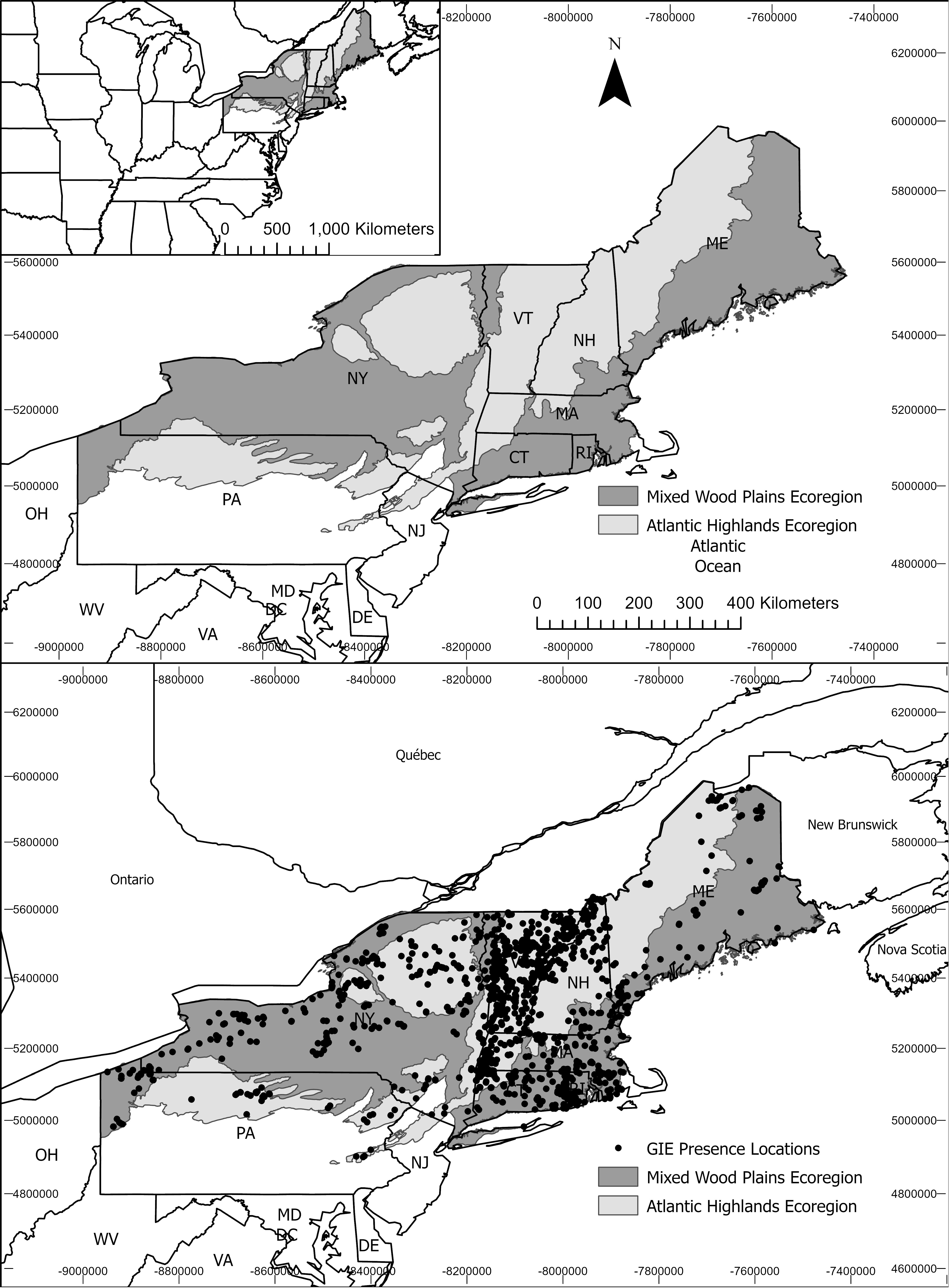
Nine states (Connecticut, Maine, Massachusetts, New Hampshire, New Jersey, New York, Pennsylvania, Rhode Island, and Vermont) spanning the Atlantic Highlands and Mixed Wood Plains EPA Level II ecoregions [45] in the northeastern United States (Figure 1) defined our modeling extent. All states were modeled in both Ecoregions except New Jersey (Atlantic Highlands Ecoregion only) and Rhode Island (Mixed Wood Plains Ecoregion only). These ecoregions are partitioned by physical and biological factors in a hierarchical framework that identifies ecologically similar regions [45]. We developed separate models that predict suitability of the landscape for GIE occurrence in 30 m × 30 m pixels across each ecoregion extent.

2.2. Allocation of Presence Dataset

We developed our models with presence data extracted from mapped, field-verified GIE locations (1981–2020) provided as X/Y coordinates by state Natural Heritage Programs (NHPs) in the study region. We filtered each NHP database for natural community types or vegetative communities verified by NHP biologists to be fully or partially sustained by groundwater (Table 1). Some NHPs provided polygon shapefiles estimating the extent of the focal vegetation community. Our modeling approach required occurrence training data as X/Y coordinates, necessitating conversion of shapefile polygon features into points by calculating the polygon centroid. We then visually confirmed that each centroid fell within the polygon feature, and we reduced effects of spatial autocorrelation in our models by removing occurrence records within 2 km of other record locations. We checked our resulting training dataset for spatial sorting bias (SSB) and determined that SSB had no effect (SSB value = 1). We retained the removed data (1478 locations; 1324 in Atlantic Highlands and 154 in Mixed Wood Plains Ecoregions) for later comparison with ensemble model predictions to assess model performance. We then conducted a k-fold random holdout with five folds on the removed data to reduce spatial bias. We used the same datasets for training all models (646 locations in the Mixed Wood Plains and 1044 locations in the Atlantic Highlands; Figure 1), and we used additional independent data (296 locations: 265 in the Atlantic Highlands and 31 in the Mixed Wood Plains) for testing all models to enable comparisons of predictions among competing models.
Figure 1. Top frame: Environmental Protection Agency (EPA) Level II Ecoregions (Atlantic Highlands, Mixed Wood Plains) in 9 states of the northeastern United States. Bottom frame: Dots represent distribution of Groundwater-Influenced Ecosystems (GIEs) presence locations (1690) used as training data for the correlative distribution models. Location data used for model training and assessment was provided by state Natural Areas Programs, as indicated in Table 2. State abbreviations: Connecticut (CT), Delaware (DE), Massachusetts (MA), Maine (ME), Maryland (MD), New Hampshire (NH), New Jersey (NJ), New York (NY), Ohio (OH), Pennsylvania (PA), Rhode Island (RI), Vermont (VT), Virginia (VA), and West Virginia (WV). All states were modeled in both Ecoregions except New Jersey (Atlantic Highlands Ecoregion only) and Rhode Island (Mixed Wood Plains Ecoregion only).
Water 15 04035 g001

2.3. Environmental Covariates

We selected environmental covariates to use in our models by reviewing the literature describing groundwater systems [1,9,19,20,22,49]. We chose environmental covariates that can be used to identify locations where groundwater is within 1 m of the land surface or is being discharged at the land surface. The two focal ecoregions have similar climatic regimes [45]; therefore, we focused on environmental variables that describe the geology and topography [50]. We chose five variables derived from topographic data (elevation as meters above sea level, topographic wetness index [TWI], landforms, terrain roughness index, percent slope), five variables derived from geology data (surficial materials, hydric soils, soil water holding capacity, soil depth, soil permeability), and one variable derived from vegetation data (normalized difference vegetative index, or NDVI) as predictor variables (Table 2). We calculated NDVI with Landsat 8 Surface Reflectance imagery collected during July and August in 2012 and 2020, months when much of the northeastern U.S. experienced Palmer Drought Index drought conditions (Source: https://www.ncdc.noaa.gov/temp-and-precip/drought/historical-palmers/, accessed on 1 December 2021; [51]). We selected periods of drought for NDVI calculations because we hypothesized that vegetation in areas with groundwater connections would retain greater greenness that would be distinguishable in imagery. We used Google Earth Engine (https://earthengine.google.com/, accessed on 1 December 2021; [52]) to retrieve and combine the selected imagery into one composite image by calculating the median NDVI value for each 30 m pixel. All data layers were clipped to the Mixed Wood Plains and Atlantic Highlands EPA Level II Ecoregions [45] and resampled to a common resolution of 30 m pixels.

2.4. Model Development and Evaluation

No single modeling approach will fit every scenario [34], and using only one approach may bias results [35,36,37]. Therefore, we modeled landscape suitability for GIEs in our study areas with four correlative distribution modeling approaches. We developed two classical regression models (Generalized Additive Models, or GAMs; Generalized Linear Models, or GLMs) and two machine learning models (Maximum Entropy, or MaxEnt; Random Forest) that are extensively used in species distribution modeling [32,53]. Generalized Additive and Linear Models have commonly been used as correlative distribution modeling methods [32,54,55]. These models have an established statistical foundation for understanding ecological relationships, with GLMs fitting linear terms to parametric distributions and with GAMs smoothing data to fit terms in non-linear functions with non-parametric distributions. MaxEnt [31] is a machine learning algorithm that estimates distributions by finding the distribution with maximum entropy given the environmental conditions at occurrence locations. MaxEnt is a correlative distribution modeling method that performs well when compared with similar methods [32,56]. Random Forest [30] is a modification of classification and regression trees that ensembles decision trees to make predictions. Like MaxEnt, Random Forest has also performed well when compared against similar methods [57]. We averaged the predictions from these four models to create one consensus or ensemble model for each ecoregion.
We developed our models with packages in R (version 1.4.1106), including ‘mgcv’ (GAM; [58]), ‘random forest’ (random forest; [59]), and ‘dismo’ (MaxEnt; [60]). The GIE occurrence data were presence-only; therefore, we generated 10,000 pseudo-absence locations [29] by randomly sampling across the study area. We partitioned occurrence and pseudo-absence data into training and testing datasets with a K-fold cross-validation with five folds. None of the predictor variables were highly correlated (R2 < 0.60). For GAM and GLM models, all predictor variables were standardized before model fitting.
We evaluated model prediction accuracy with Area Under the Curve (AUC) estimates, Cohens Kappa statistic, sensitivity and specificity rates, deviance, and the True Skill Statistic (TSS). AUC estimates the predictive accuracy of distribution models derived from presence-absence data [61], with estimates of 0.5 indicating model performance no better than random and with estimates closer to 1.0 indicating good model performance. We considered model AUC estimates of ≥0.70 to be informative [62]. Cohens Kappa statistic measures inter-rater reliability, or precision, with scores ranging from 0 (no agreement) to 1 (complete agreement) [63]. We considered a Kappa statistic of ≥0.50 to be informative [64]. Deviance is a measure of goodness-of-fit, with a smaller deviance indicating better fit to the model. The TSS provides a threshold-dependent measure of accuracy by accounting for both sensitivity (proportion of correctly identified positive detections) and specificity (proportion of correctly identified negative detections), while independent of the number of sample points used to build the model [65]. The TSS is scored from −1.0 (no better than random) to +1.0 (perfect agreement) [65]. We considered a TSS score ≥ 0.50 to indicate a good model fit. We further estimated sensitivity (true positive rate) and specificity (true negative rate) values for each competing model to evaluate model accuracy, and we considered values ≥ 0.70 to be informative.

2.5. Model Validation

We validated the models by comparing model predictions to the withheld occurrence dataset and on-site evaluations. We identified a threshold for a well-performing model by partitioning the predicted suitability values for each consensus model and ecoregion into 10 bins using natural breaks and then identified pixels within the upper two bins (i.e., thresholds that represent greatest predicted suitability) of GIE suitability predictions. We used our withheld dataset to compare against these two upper bins for each consensus ensemble model in each ecoregion. If a withheld presence location fell within the upper two bins of our consensus models, we considered the model prediction to be correct. We prioritized pixels in the top two bins for on-site evaluations, focusing on federal and state-owned public lands owing to accessibility and time limitations. Locations for these evaluations were randomly selected within accessible areas that were predicted to be highly suitable (≥0.70).
We conducted three types of on-site evaluations during June–August 2020–2022. In areas predicted to be suitable for GIEs in or around NWI-mapped wetlands, we used a site rapid assessment composed of questions (Figure 2) and measurements to assess vegetation, topography, soils, and presence of water features characteristic of wetland GIEs [2,15,66,67]. At sites in areas predicted to be suitable for GIEs near a stream or river, the rapid assessment included questions modified for rivers and streams (Figure 2). Our rapid assessments were guided by previously developed assessments (e.g., U.S. Forest Service Gen. Tech. Report WO-86a) and in consultation with professional wetland ecologists and hydrogeologists. We inferred a high likelihood of suitable conditions for GIE “presence” at locations in our validation dataset where at least four of six rapid assessment questions were answered affirmatively. In addition to the rapid assessment survey, we measured water surface temperature at the sites with a handheld infrared (IR) camera (Forward Looking InfraRed (FLIR) E6, Teledyne FLIR LLC; [18,68]. We used the IR camera to scan wetland (e.g., out 25 m from initial XY location in each cardinal direction), streams, and river edges at the site (e.g., out from the initial XY location to extent of predicted suitable area up and down stream or river) to locate where cold water (≤12 °C) contrasted with background temperatures (≥18 °C), indicating groundwater discharge. If our IR camera detected these temperature anomalies (Supplementary Materials, Figure S1), we considered the site to be a “presence” location in our validation dataset.

2.6. Model Agreement

We compared areas predicted to be suitable for GIE presence in the four models by applying two thresholds (N, 0.70) to identify pixels as “suitable” or “unsuitable”. The “N” threshold was calculated as the upper two (i.e., indicating greatest suitability) of 10 bins partitioned by natural breaks in the range of predicted suitability values. The “0.70” threshold indicated pixels with a suitability score ≥ 0.70. We compared the model outputs to identify pixels meeting both thresholds. We calculated the total area (hectares) where each of the four models satisfied both threshold methods in each ecoregion. Suitable areas for each model were assigned a unique number that identified which models met both thresholds for each pixel. We assigned suitable areas in GAM models a value of 0001, GLM models a value of 0010, MaxEnt models a value of 0100, and Random Forest models a value of 1000. The summed pixel value identified the models that were in agreement. For example, a pixel value of 0111 indicated that the GAM, GLM, and Maxent models were in agreement for that pixel (i.e., 0001 + 0010 + 0100 = 0111), whereas the Random Forest model did not predict that pixel was suitable for occurrence of a GIE in this example.

2.7. Ensemble Model

We created a consensus ensemble model for each ecoregion from the four individual models by calculating the mean suitability score for each pixel. We calculated the standard deviation, range, and coefficient of variation within each pixel in the modeled domains to identify areas of variability in the predictions of the consensus models for each ecoregion. We used our withheld occurrence datasets and our on-site validation surveys to estimate accuracy of the ensemble models by comparing the pixel values for the withheld occurrence locations with the predicted suitable areas partitioned by the 10 natural breaks threshold (i.e., where the upper two bins were considered suitable). Additionally, we determined the wetland system type associated with predicted GIE occurrence probability by overlaying the NWI database of mapped wetlands and deep-water habitats on the predicted suitable areas. We also used this approach to identify where our models predicted high suitability for GIEs, yet there are no NWI-mapped wetlands.

3. Results

3.1. Classical Regression Models (GAM, GLM)

Two categorical surficial material variables (surfmat3:eolian sediments, mostly dune sand, thick; and surfmat29:glaciofluvial ice-contact sediments, mostly sand and gravel, thick), and four continuous variables (elevation, TWI, soil water holding capacity, soil permeability) were significant variables fitted with the GAM model for the Mixed Wood Plains Ecoregion (Table 3). Similarly, surfmat3, surfmat29, elevation, hydric soil, and soil permeability were important variables in the fitted GLM model for the Mixed Wood Plains Ecoregion (Table 4). Significant variables in the GAM-fitted model for the Atlantic Highlands Ecoregion included elevation, hydric soil, terrain roughness index, TWI, slope, soil depth, soil water holding capacity, and NDVI (Table 5). The fitted GLM model for the Atlantic Highlands Ecoregion included surfmaterials32 (colluvial sediments and residual material), elevation, hydric soil, terrain roughness index, slope, soil water holding capacity, and NDVI (Table 6). In the Mixed Wood Plains Ecoregion, GAM and GLM models both indicated that areas with a large percentage of hydric soil and high soil permeability had the greatest probability of GIE presence. In the Atlantic Highlands Ecoregion, hydric soil, TWI, soil water holding capacity, and elevation were important predictors by GAM models, whereas the GLM Atlantic Highlands Ecoregion model predicted GIE presence with variables representing hydric soils, NDVI, elevation, and slope (Table 6).

3.2. Machine Learning Models (MaxEnt, Random Forest)

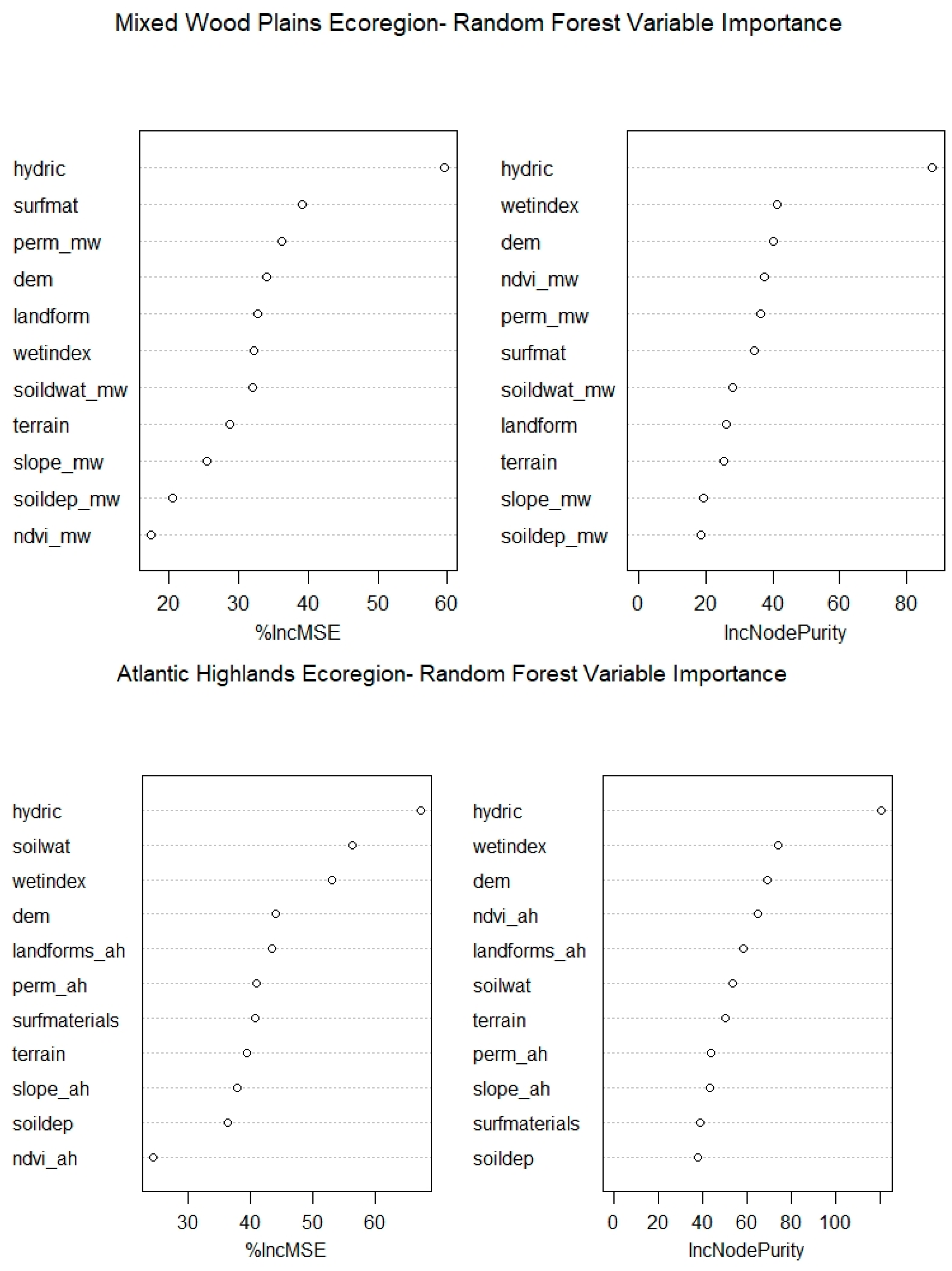
In the Mixed Wood Plains Ecoregion, the Random Forest model estimated that hydric soil, surface materials, soil permeability, and elevation contributed the greatest increase (35–60%) in percent mean square error, while hydric soil, TWI, elevation, NDVI, soil permeability, and surface materials had the greatest increases in node purity (Figure 3). The Maxent model for the Mixed Wood Plains Ecoregion estimated that hydric soil, landforms, soil permeability, and surface materials contributed the most (10–55%) to the overall fit of the model (Figure 4). The Random Forest model for the Atlantic Highlands Ecoregion estimated that hydric soil, soil water holding capacity, and TWI had the greatest increase (55–68%) in percent mean square error, while hydric soil, TWI, elevation, NDVI, and landforms had the greatest increases in node purity (Figure 3). The Maxent model for the Atlantic Highlands Ecoregion estimated that hydric soil, landforms, and TWI had the greatest contribution to the overall fit of the model (Figure 5). In both ecoregions, variable importance was similar for Random Forest and Maxent models, with hydric soil, TWI, landforms, and elevation having the greatest influence on GIE presence.

3.3. Evaluation of Models

In the Mixed Wood Plains Ecoregion, all four model AUC values exceeded >0.85, with the Random Forest model performing best (Table 7). Sensitivity and specificity (>0.70) and TSS (>0.60) values indicate the four models were informative (Table 7). The GAM model had the largest Kappa statistic and specificity value (Table 7). In the Atlantic Highlands Ecoregion, AUC values exceeded 0.85, sensitivity was >0.70, and specificity was >0.70 for all four models (Table 7). AUC, Kappa statistic, specificity, and deviance values were best for the Random Forest model, whereas the Maxent model had the greatest sensitivity among the models. The TSS was largest for the Random Forests and MaxEnt models (Table 7). Among models in both ecoregions, AUC and sensitivity values were consistently large; however, specificity values were consistently smaller for the Atlantic Highlands Ecoregion models. Overall, Random Forest and Maxent were the best-performing models for both ecoregions; however, GAM and GLM models can also be considered informative.

3.4. Model Agreement

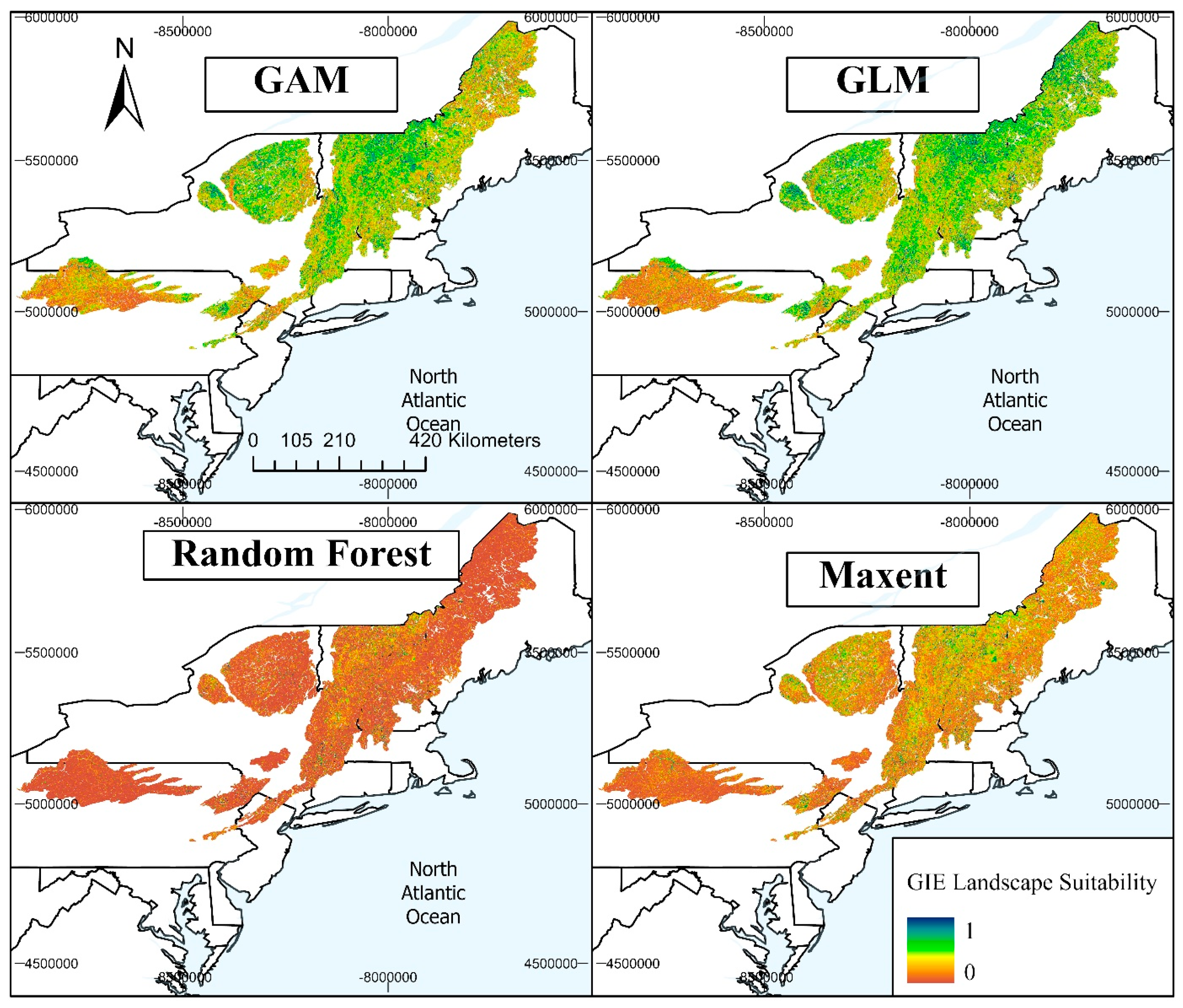
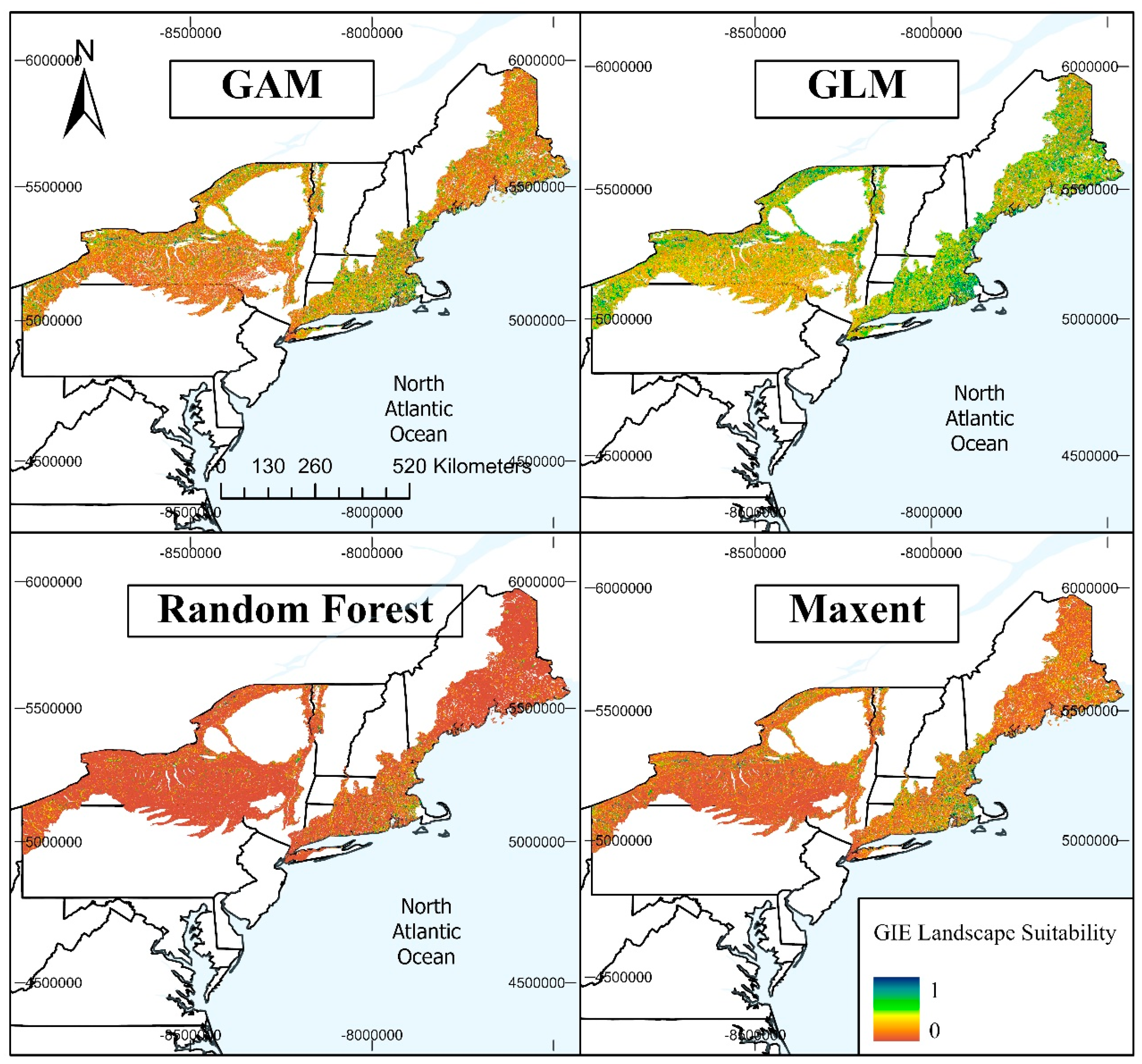
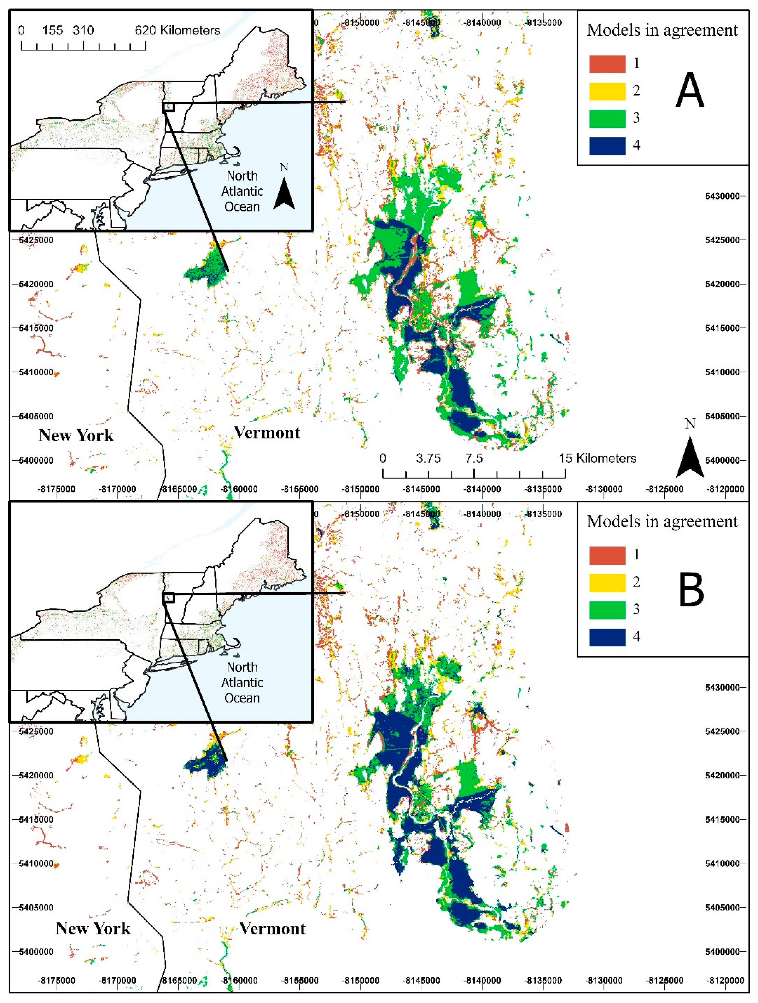
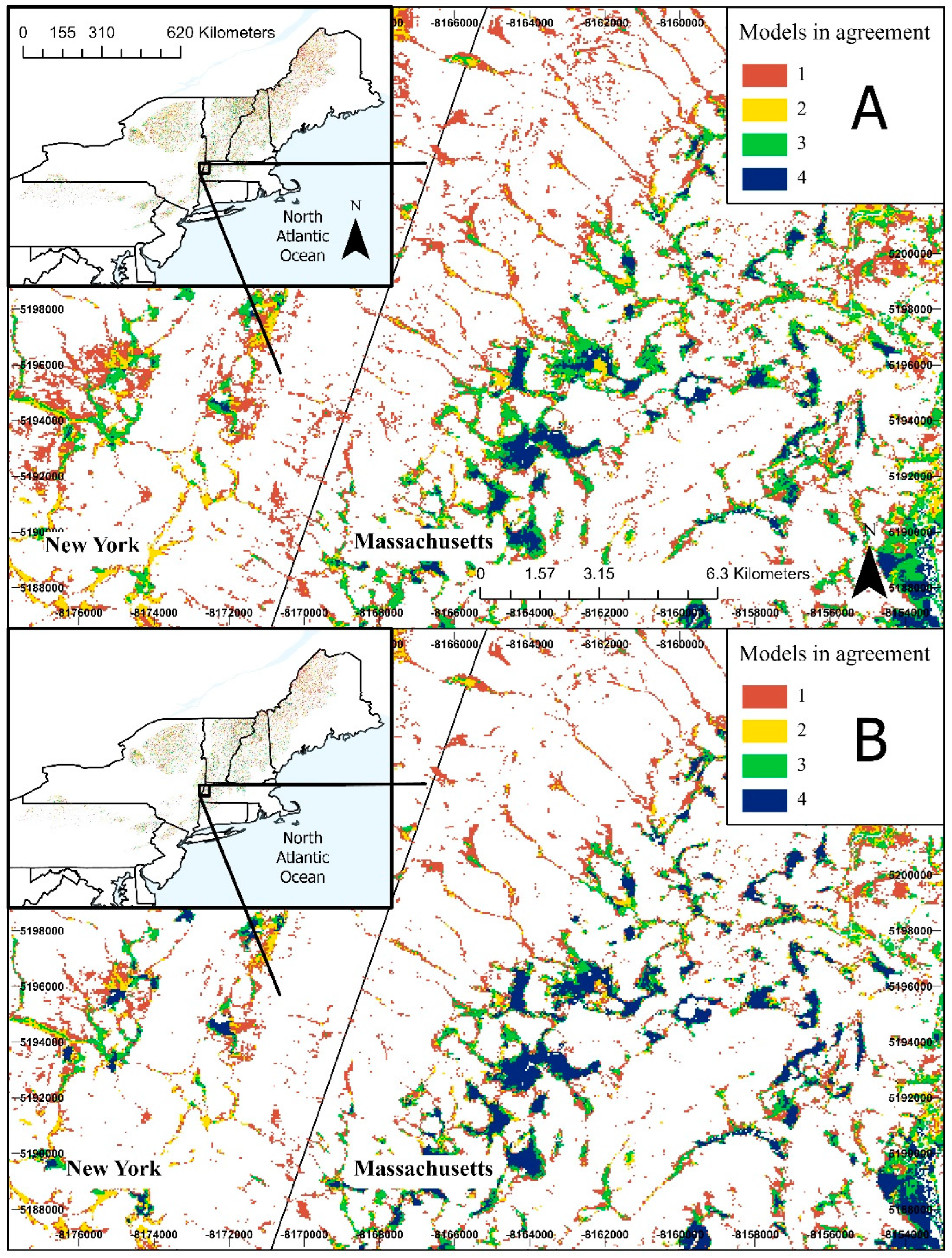
Less than 1% of the total modeled area in the two ecoregions was predicted to be suitable for GIEs, with 0.29% (53,285 ha) of the Mixed Wood Plains Ecoregion and 0.41% (61,710 ha) of the Atlantic Highlands Ecoregion predicted suitable based on the Natural Breaks threshold (Table 8). The four modeling approaches were variable in their predictions (Figure 6 and Figure 7). Approximately 1% of the modeled area within each ecoregion was predicted suitable by three models, while 1–3% was predicted suitable by two models (Figure 8 and Figure 9; Table 8; Supplementary Materials, Figures S2 and S3).
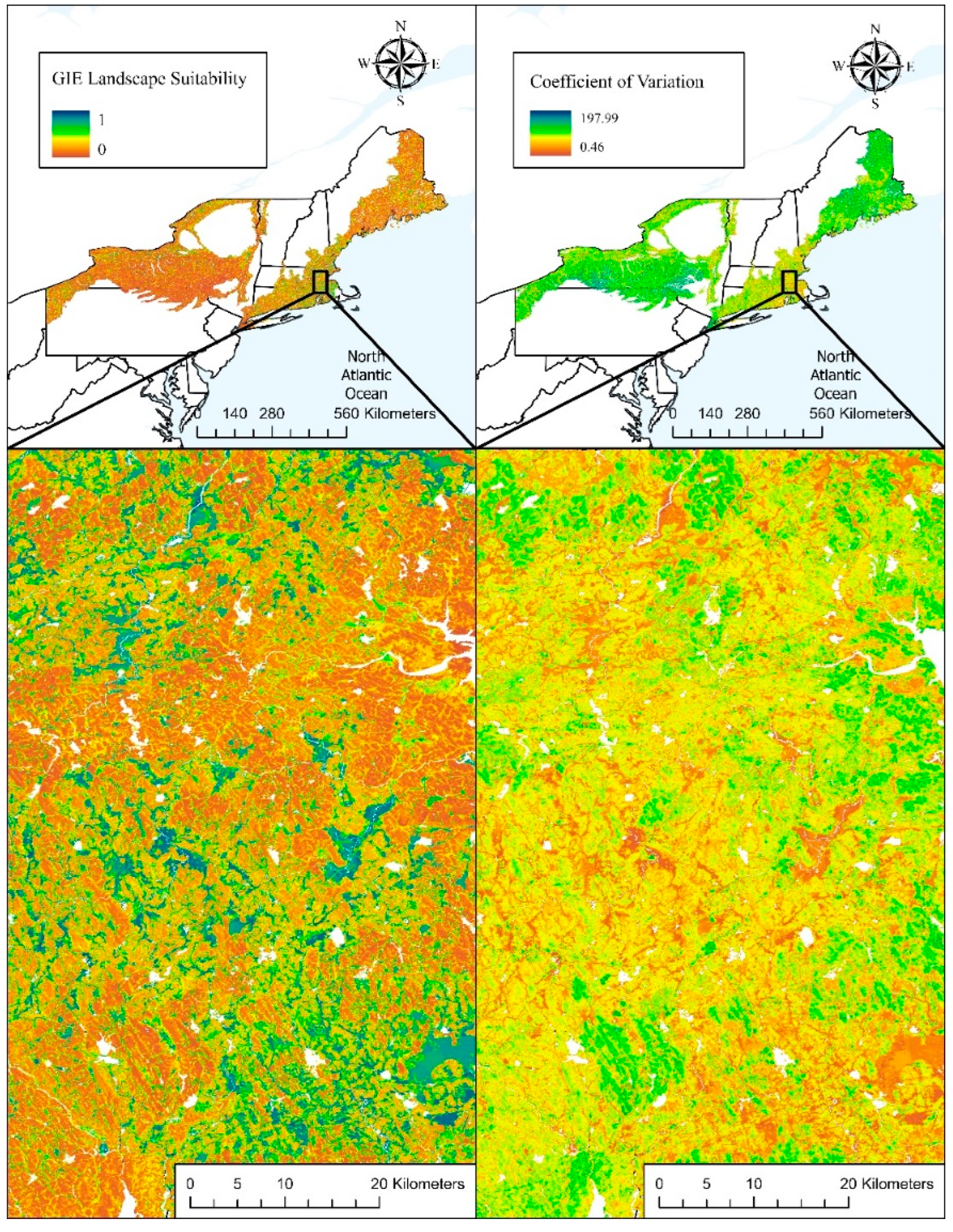
We observed geographic trends in model agreement. For example, in the Atlantic Highlands Ecoregion, the largest clusters of suitable (top 10th percentile) areas in the ensemble model occurred in northern Vermont and New Hampshire. There was also the least amount of variability among model predictions (coefficient of variation < 25; Figure 10; Supplementary Materials, Figure S4) in this region. In the Mixed Wood Plain ecoregion, clusters of predicted suitable area (suitability in the upper 10th percentile) occurred where there was the most certainty among model predictions (i.e., smallest coefficient of variation) based on the coefficient of variation for each pixel (coefficient of variation value < 25; Figure 11; Supplementary Materials, Figure S5).

3.5. Ensembled Model

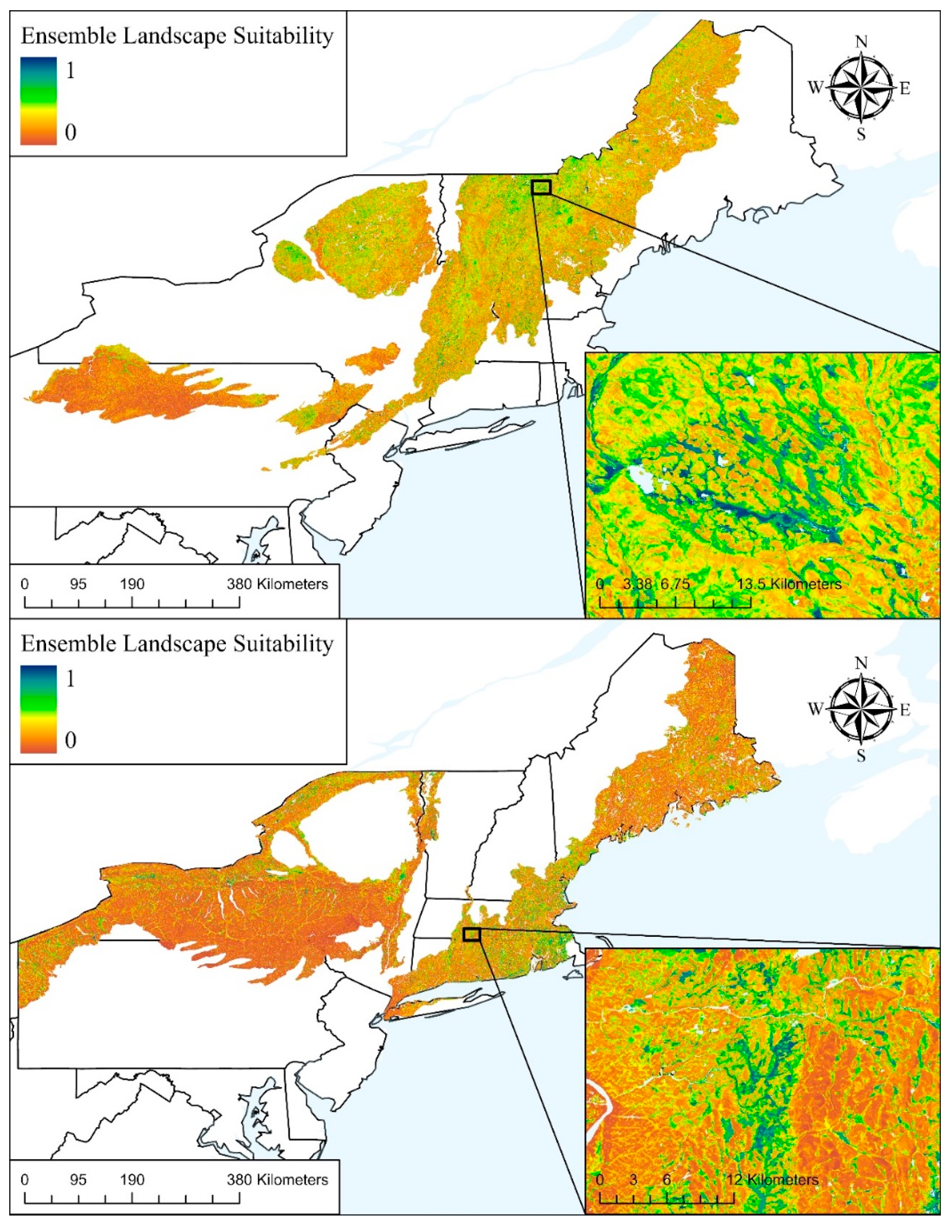
The Mixed Wood Plains Ecoregion ensemble model was 81% accurate, based on 91 validation points from 60 on-site field surveys and 31 points drawn from the withheld dataset. The Atlantic Highlands Ecoregion ensemble model was 80% accurate, based on 353 validation points from 88 on-site field surveys and 265 points drawn from the withheld dataset. Based on the Natural Break threshold (N), the majority of areas predicted to be suitable for GIEs in the Mixed Wood Plains Ecoregion occurred in Massachusetts, New York, and Connecticut, with 153,647 ha predicted as suitable (Table 9; Figure 12). In the Atlantic Highlands Ecoregion, the majority of areas predicted to be suitable for GIEs occurred in Vermont, New Hampshire, and New York, with 168,888 ha predicted as suitable (Table 9; Figure 12).
In both ecoregions, the majority of areas predicted to be suitable for GIE occurrence occurred in mapped NWI wetlands and most frequently in the freshwater forested/shrub wetland and freshwater emergent wetland types (Table 10). NWI-mapped riverine wetlands predicted to contain GIEs accounted for 1.8% of the total predicted GIE-suitable area in the Mixed Wood Plains Ecoregion and 3.4% in the Atlantic Highlands Ecoregion. In the Mixed Wood Plains Ecoregion, 5.4% of the mapped NWI wetlands were predicted to contain suitable conditions for GIEs, whereas 9.3% of the mapped NWI wetlands were predicted to contain suitable conditions for GIEs in the Atlantic Highlands Ecoregion (Table 10). Our ensemble models also identified areas predicted to be suitable for GIEs (Mixed Wood Plains 16,354 ha; Atlantic Highlands 28,092 ha) but that are not currently mapped as wetlands in the NWI. Overall, 138,164 ha were predicted suitable for GIEs in mapped NWI wetlands in the Mixed Wood Plains Ecoregion, and 140,818 ha were predicted suitable for GIEs in mapped NWI wetlands in the Atlantic Highlands Ecoregion.

4. Discussion

4.1. Development and Reliability of Ensembled Correlative Distribution Models

Our field-validated ensemble consensus models predicting the probability of conditions suitable for GIEs in the Atlantic Highlands and Mixed Wood Plains EPA Level II Ecoregions in the northeastern United States indicate that GIEs may be relatively uncommon in this region. The rarity of GIEs in the landscape was also indicated by distribution maps developed in Oregon [1] and California [11]. Evaluation metrics, such as AUC, TSS, Kappa statistic, and sensitivity and specificity rates, indicated that each of the modeling methods (GAM, GLM, Maxent, Random Forest) performed well individually as well as in combination, supporting the utility of ensemble correlative distribution models to predict the suitability of the landscape for GIEs. In the Atlantic Highlands Ecoregion, suitable landscapes for GIE presence are in greatest occurrence in mountainous terrain in northern Vermont and New Hampshire and in northeastern New York’s Adirondack Mountains. Most of the suitable landscape in the Mixed Wood Plains Ecoregion was predicted to be in Massachusetts, Connecticut, and northern New York. The predictions of where suitable landscapes occur in both ecoregions are affected by the abundance and distribution of verified presence locations in the NHP datasets from Vermont, New Hampshire, and Massachusetts. In contrast, verified presence locations are less abundant in datasets provided by Maine and Pennsylvania NHPs, which may result in underrepresenting the true occurrence of GIEs and therefore contribute to underestimates of suitable areas in those states.
The large spatial extent of our models also limited the number of environmental predictors we could include as variables to those with full coverage across the study area. Variables available at greater spatial resolution over smaller extents (e.g., water table depth) also may have improved the accuracy of ensemble models. Our ensemble model resolution was 30-m pixels, which likely overlooked small GIEs such as springs. Increased resolution and spatial accuracy of data for important variables could result in more accurate models by reducing omission and commission errors. Despite these limitations, our ensemble correlative distribution model is a reliable, novel approach for estimating and mapping landscape suitability for GIEs across broad spatial scales that could increase understanding of where these systems are distributed, particularly within wetlands and streams.

4.2. Important Variables in Ensembled Models

In all of the individual models (GLM, GAM, Maxent, Random Forest), hydric soil was the most important predictor (>75%) of conditions suitable for GIE presence. Hydric soils are consistently saturated soils, with anoxic soils occurring in the upper portion of the soil profile [69]. Topographic wetness index (ranging from 0 to 15) was also an important predictor, with values >8 most correlated with GIE presence. Other studies conducted in New York [70] and Iran [71] also found an association between groundwater-dependent ecosystems and topographic wetness. Additionally, we identified differences in important predictor variables in the Atlantic Highlands and Mixed Wood Plains Ecoregions. Our models predicted that environmental variables related to geology (e.g., hydric soil, soil permeability, surface materials, soil water holding capacity) accounted for the majority of important predictors of conditions suitable for GIE presence in the Mixed Wood Plains Ecoregion, while a combination of variables related to geology and topography (e.g., hydric soil, topographic wetness index, landforms, elevation, soil water holding capacity) were important in the Atlantic Highlands Ecoregion. The Atlantic Highlands Ecoregion is a heavily forested, cool, humid, predominantly mountainous region with many lakes and streams and underlain by glacial sediments [45]. Topographic relief in the Atlantic Highlands Ecoregion shapes local groundwater recharge and discharge zones [72]. In contrast, the Mixed Wood Plains Ecoregion is underlain by glacial sediments with flat lake plains, rolling till plains, hummocky stagnation moraines, hills, and a mosaic of land cover types [45]. The abundance of hills and depressions in the Mixed Wood Plains Ecoregion promotes the presence of lakes and wetlands [45], where groundwater flow is likely controlled by highly permeable geologic deposits [72], suggesting an influence of geology on GIEs. The distribution of fens in the Mixed Wood Plains Ecoregion in New York is related to the occurrence of carbonate geology and soil properties [70], similar to our findings. Other GIE mapping efforts in the western United States also hypothesized the importance of geology and found geological variables to be important indicators [1,11]. We did not include climatic variables as predictors in our models; however, areas predicted to be suitable for GIEs in both ecoregions coincide with areas in the Northeast that receive abundant annual precipitation based on historical measurements (USGS: https://www.usgs.gov/media/images/map-annual-average-precipitation-us-1981-2010, accessed on 1 December 2021), indicating that climate, specifically precipitation, may be an important predictor of GIE occurrence in the region. This relationship with precipitation was also noted in groundwater ecosystem mapping efforts in the Philippines [73].

4.3. Prediction of Wetlands with Groundwater Influence

Predicted suitable areas for GIEs in wetlands occur most frequently in wetlands mapped in the NWI as freshwater forested and freshwater shrub wetlands (i.e., freshwater swamps) or freshwater emergent wetlands (i.e., freshwater marshes). Mapped NWI wetlands and deep-water habitats predicted as GIEs accounted for relatively small proportions of the overall area of mapped wetland types in the two focal ecoregions, with the exception of estuarine and marine deep-water wetlands and freshwater emergent wetlands in the Atlantic Highlands Ecoregion. These wetland types occur rarely (<2000 ha) in this ecoregion. Riverine systems predicted to be suitable for GIEs also accounted for a small amount of the overall suitable area; however, twice as much riverine wetland type was predicted to be suitable for GIEs in the Atlantic Highlands Ecoregion compared with suitable areas in riverine wetlands in the Mixed Wood Plains Ecoregion.
The NWI, created to map and describe all wetland features in the United States for inventory and monitoring, is known to have commission and omission errors [74,75,76]. Our ensemble models identified areas predicted to be suitable for GIEs that are omitted from the NWI. There is no NWI modifier indicating a relationship with groundwater specifically [77], although the chemistry modifier suggests that groundwater recharge and discharge may be present. Our ensemble models used spatial data layers for variables describing geology and topography, which have functional relationships with groundwater, whereas the NWI uses information about hydroperiod and vegetation assessed from aerial photographs and ground surveys to map and classify wetlands [77]. Our ensemble modeling approach could augment the NWI mapping approach to identify wetland functions that are influential for wetland regulation and mitigation [78].

4.4. Predictions of Groundwater-Influenced Thermal Refugia in Streams and Rivers

Understanding where groundwater contributes to stream and river base flow can inform the management of species dependent on cold water, particularly where warm water temperatures reduce suitable habitat for these species [7,79]. River or stream reaches that receive groundwater as baseflow can be buffered from warm ambient air temperatures in the summer and provide thermal refugia (i.e., cold water habitat) for thermally sensitive aquatic species such as brook trout [80], Atlantic salmon [7], and dwarf wedgemussel [6]. Our models predicted groundwater influence in approximately 318 km of river and stream reaches (1710 unique reaches; 0.9% of total mapped reaches) in Maine. Some of these streams may provide high-quality habitat for the federally endangered Atlantic salmon, whose remaining wild populations in the United States are found in a small number of stream and river reaches in Maine [81]. Our model predictions of reaches with predicted groundwater influence agree (75% agreement; 787 of 1054 reaches) with predictions of reaches with high base flow, based on stream flow and geology variables [81], that may provide thermal refugia for Atlantic salmon.
In addition to identifying stream and river reaches with potential suitability for groundwater influence locally, our modeling approach identifies areas of potential suitability for groundwater influence across regions, which may contribute to the management of broadly distributed species that rely on groundwater presence. For example, brook trout, an economically important species that is widely distributed across the northeastern U.S., has narrow thermal tolerances [82], restricting its native populations to cooler streams and rivers that may receive groundwater baseflow. In lentic systems and at a local scale, wetlands that are connected to groundwater have been observed to have a high diversity of unique plant species, especially in wetlands where groundwater is the dominant water source (fens; [83]). In New York and New Hampshire, 7% and 13.7% of the state’s rare flora occur in groundwater-connected systems, respectively [84]. Our ensemble model results may indicate additional areas with these sensitive plant communities. The number of uncommon, rare, federally threatened, and federally endangered plant species that occur in groundwater-influenced systems is notable [84]. Our ensemble correlative distribution modeling approach could lead to a more comprehensive inventory and monitoring of these species.

4.5. Future Applications and Improvements

Ensembled correlative distribution models can be used to map GIEs across broad geographic landscapes with relatively high accuracy. This approach may also be reliable in other geographic areas. Geological and topographical variables are important variables in the Atlantic Highlands and Mixed Wood Plains Ecoregion models; identifying environmental variables in other regions could be an important step in applying this approach beyond the northeastern United States. With advancements in remote sensing technology, climatic and geospatial environmental data are becoming more widely accessible and at broader spatial extents. For example, medium-resolution Advanced Spaceborne Thermal Emission and Reflection Radiometer (ASTER) satellite imagery can be used to characterize elevation, geology, and soil environmental variables [2], which are important indicators of GIEs [85,86]. Models developed to predict groundwater-influenced systems in other ecoregions may be improved as additional high-resolution environmental spatial data are available.
The ensemble correlative distribution modeling approach is data-driven, and similar to our models, the quality of presence data and environmental variables can affect model accuracy [26]. Bias in the abundance and distribution of presence locations [87], as well as the selection of data for environmental variables included in the models [88], can affect model predictions and contribute to commission and omission errors [26]. Future work could benefit from the creation of region-specific rapid assessment protocols to identify GIEs for use in statistical model calibration and validation. As groundwater-influenced ecosystems are increasingly threatened by anthropogenic and climatic stressors [16], understanding where these systems occur in the landscape could be important to their conservation and sustainability. Our ensemble modeling approach provides a transferable, interpretable, and replicable tool for this purpose.

Supplementary Materials

The following supporting information can be downloaded at: https://www.mdpi.com/article/10.3390/w15234035/s1, Figure S1: Thermal Imaging of Groundwater; Figure S2: Model Agreement in Mixed Wood Plains Ecoregion; Figure S3: Model Agreement in Atlantic Highlands Ecoregion; Figure S4: Atlantic Highlands Ecoregion Model Uncertainty; Figure S5: Mixed Wood Plains Ecoregion Model Uncertainty.

Author Contributions

S.D.S., A.S.R. and C.S.L. conceived the ideas and designed methodology; S.D.S. collected the data; S.D.S. analyzed the data; and S.D.S. led the writing of the manuscript. All authors have read and agreed to the published version of the manuscript.

Funding

This project was funded by the University of Maine and the Maine Department of Inland Fisheries and Wildlife through the Cooperative Agreement with the U.S. Geological Survey, the Maine Cooperative Fish and Wildlife Research Unit, the Maine Agricultural and Forest Experiment Station, and the U.S. Geological Survey Science Support Program.

Data Availability Statement

Data (Snyder et al., 2023) are available from ScienceBase: https://doi.org/10.5066/P97DJ8E6.

Acknowledgments

The authors thank the anonymous reviewers for reviewing the manuscript. We thank the U.S. Fish and Wildlife Service, the Maine Bureau of Parks and Land, and the University of Maine for providing access to their lands for on-site fieldwork to validate the models. Field-collected data used in this study and model rasters are available in the Sciencebase record https://doi.org/10.5066/P97DJ8E6. Any use of trade, firm, or product names is for descriptive purposes only and does not imply endorsement by the U.S. Government.

Conflicts of Interest

The authors declare no conflict of interest.

References

  1. Brown, J.; Bach, L.; Aldous, A.; Wyers, A.; DeGagné, J. Groundwater-Dependent Ecosystems in Oregon: An Assessment of their Distribution and Associated Threats. Front. Ecol. Environ. 2011, 9, 97–102. [Google Scholar] [CrossRef]
  2. Pérez Hoyos, I.C.; Krakauer, N.Y.; Khanbilvardi, R.; Armstrong, R.A. A Review of Advances in the Identification and Characterization of Groundwater Dependent Ecosystems Using Geospatial Technologies. Geosciences 2016, 6, 17. [Google Scholar] [CrossRef]
  3. Glasser, S.; Gauthier-Warinner, J.; Keely, J.; Gurrieri, J.; Tucci, P.; Summers, P.; Wireman, M.; McCormack, K. Technical Guide to Managing Ground Water Resources; United States Department of Agiculture: Washington, DC, USA, 2007.
  4. Rohde, M.M.; Froend, R.; Howard, J. A Global Synthesis of Managing Groundwater Dependent Ecosystems under Sustainable Groundwater Policy. Groundwater 2017, 55, 293–301. [Google Scholar] [CrossRef]
  5. Van Grinsven, M.; Mayer, A.; Huckins, C. Estimation of Streambed Groundwater Fluxes Associated with Coaster Brook Trout Spawning Habitat. Groundwater 2012, 50, 432–441. [Google Scholar] [CrossRef]
  6. Rosenberry, D.O.; Briggs, M.A.; Voytek, E.B.; Lane, J.W. Influence of Groundwater on Distribution of Dwarf Wedgemussels (Alasmidonta heterodon) in the Upper Reaches of the Delaware River, Northeastern USA. Hydrol. Earth Syst. Sci. 2016, 20, 4323–4339. [Google Scholar] [CrossRef]
  7. Kurylyk, B.L.; MacQuarrie, K.T.B.; Linnansaari, T.; Cunjak, R.A.; Curry, R.A. Preserving, Augmenting, and Creating Cold-Water Thermal Refugia in Rivers: Concepts Derived from Research on the Miramichi River, New Brunswick (Canada). Ecohydrology 2015, 8, 1095–1108. [Google Scholar] [CrossRef]
  8. Eamus, D. Identifying Groundwater Dependent Ecosystems: A Guide for Land and Water Managers; Land & Water Australia: Perth, Australia, 2009. [Google Scholar]
  9. Hoyos, I.C.P. Identification of Phreatophytic Groundwater Dependent Ecosystems Using Geospatial Technologies. Ph.D. Thesis, The City College of New York, New York, NY, USA, 2016. [Google Scholar]
  10. Fauvet, G.; Claret, C.; Marmonier, P. Influence of Benthic and Interstitial Processes on Nutrient Changes along a Regulated Reach of a Large River (Rhône River, France). Hydrobiologia 2001, 445, 121–131. [Google Scholar] [CrossRef]
  11. Howard, J.; Merrifield, M. Mapping Groundwater Dependent Ecosystems in California. PLoS ONE 2010, 5, e11249. [Google Scholar] [CrossRef]
  12. Aldous, A.; Bach, L. Protecting Groundwater-Dependent Ecosystems: Gaps and Opportunities. Natl. Wetl. Newsl. 2011, 33, 19–22. [Google Scholar]
  13. Le Maitre, D.C.; Colvin, C.A. Assessment of the Contribution of Groundwater Discharges to Rivers Using monthly flow statistics and Flow Seasonality. Water SA 2008, 34, 549–564. [Google Scholar] [CrossRef]
  14. Güntner, A.; Stuck, J.; Werth, S.; Döll, P.; Verzano, K.; Merz, B. A Global Analysis of Temporal and Spatial Variations in Continental Water Storage. Water Resour. Res. 2007, 43, W05416. [Google Scholar] [CrossRef]
  15. Kløve, B.; Ala-aho, P.; Bertrand, G.; Boukalova, Z.; Ertürk, A.; Goldscheider, N.; Ilmonen, J.; Karakaya, N.; Kupfersberger, H.; Kvœrner, J.; et al. Groundwater Dependent Ecosystems. Part I: Hydroecological Status and Trends. Environ. Sci. Policy 2011, 14, 770–781. [Google Scholar] [CrossRef]
  16. Kløve, B.; Ala-Aho, P.; Bertrand, G.; Gurdak, J.J.; Kupfersberger, H.; Kværner, J.; Muotka, T.; Mykrä, H.; Preda, E.; Rossi, P.; et al. Climate Change Impacts on Groundwater and Dependent Ecosystems. J. Hydrol. 2014, 518, 250–266. [Google Scholar] [CrossRef]
  17. Barron, O.V.; Emelyanova, I.; Van Niel, T.G.; Pollock, D.; Hodgson, G. Mapping Groundwater-Dependent Ecosystems Using Remote Sensing Measures of Vegetation and Moisture Dynamics. Hydrol. Process. 2014, 28, 372–385. [Google Scholar] [CrossRef]
  18. Barclay, J.R.; Briggs, M.A.; Moore, E.M.; Starn, J.J.; Hanson, A.E.H.; Helton, A.M. Where Groundwater Seeps: Evaluating Modeled Groundwater Discharge Patterns with Thermal Infrared Surveys at the River-Network Scale. Adv. Water Resour. 2022, 160, 104108. [Google Scholar] [CrossRef]
  19. Doody, T.M.; Barron, O.V.; Dowsley, K.; Emelyanova, I.; Fawcett, J.; Overton, I.C.; Pritchard, J.L.; Van Dijk, A.I.; Warren, G. Continental Mapping of Groundwater Dependent Ecosystems: A Methodological Framework to Integrate Diverse Data and Expert Opinion. J. Hydrol. Reg. Stud. 2017, 10, 61–81. [Google Scholar] [CrossRef]
  20. Hoyos, I.P.; Krakauer, N.; Khanbilvardi, R. Random Forest for Identification and Characterization of Groundwater Dependent Ecosystems. WIT Trans. Ecol. Environ. 2015, 196, 89–100. [Google Scholar]
  21. Santos, M.J.; Smith, A.B.; Dekker, S.C.; Eppinga, M.B.; Leitão, P.J.; Moreno-Mateos, D.; Morueta-Holme, N.; Ruggeri, M. The Role of Land Use and Land Cover Change in Climate Change Vulnerability Assessments of Biodiversity: A Systematic Review. Landsc. Ecol. 2021, 36, 3367–3382. [Google Scholar] [CrossRef]
  22. Werstak, C.E.; Housman, I.; Maus, P.; Fisk, H.; Gurrieri, J.; Carlson, C.P.; Johnston, B.C.; Stratton, B.; Hurja, J.C. Groundwater-Dependent Ecosystem Inventory Using Remote Sensing; United States Department of Agriculture: Washington, DC, USA, 2012.
  23. Elmore, A.J.; Mustard, J.F.; Manning, S.J. Regional Patterns of Plant Community Response to Changes in Water: Owens Valley, California. Ecol. Appl. 2003, 13, 443–460. [Google Scholar] [CrossRef]
  24. U.S. Geological Survey. National Hydrography Dataset (ver. USGS National Hydrography Dataset (NHD)). 2016. Available online: https://www.usgs.gov/core-science-systems/ngp/national-hydrography/access-national-hydrography-products (accessed on 21 November 2022).
  25. Adhikary, P.P.; Dash, C.J. Comparison of Deterministic and Stochastic Methods to Predict Spatial Variation of Groundwater Depth. Appl. Water Sci. 2017, 7, 339–348. [Google Scholar] [CrossRef]
  26. Jarnevich, C.S.; Stohlgren, T.J.; Kumar, S.; Morisette, J.T.; Holcombe, T.R. Caveats for Correlative Species Distribution Modeling. Ecol. Inform. 2015, 29, 6–15. [Google Scholar] [CrossRef]
  27. Shabani, F.; Kumar, L.; Ahmadi, M. A Comparison of Absolute Performance of Different Correlative and Mechanistic Species Distribution Models in an Independent Area. Ecol. Evol. 2016, 6, 5973–5986. [Google Scholar] [CrossRef]
  28. McCullagh, P.; Nelder, J.A. Binary Data. In Generalized Linear Models; Springer: Berlin/Heidelberg, Germany, 1989; pp. 98–148. [Google Scholar]
  29. Elith, J.; Phillips, S.J.; Hastie, T.; Dudík, M.; Chee, Y.E.; Yates, C.J. A Statistical Explanation of MaxEnt for Ecologists. Divers. Distrib. 2011, 17, 43–57. [Google Scholar] [CrossRef]
  30. Breiman, L. Random Forests. Mach. Learn. 2001, 45, 5–32. [Google Scholar] [CrossRef]
  31. Phillips, S.J.; Anderson, R.P.; Schapire, R.E. Maximum Entropy Modeling of Species Geographic Distributions. Ecol. Model. 2006, 190, 231–259. [Google Scholar] [CrossRef]
  32. Elith, J.; Graham, C.H.; Anderson, R.P.; Dudík, M.; Ferrier, S.; Guisan, A.; Hijmans, R.J.; Huettmann, F.; Leathwick, J.R.; Lehmann, A.; et al. Novel Methods Improve Prediction of Species’ Distributions from Occurrence Data. Ecography 2006, 29, 129–151. [Google Scholar] [CrossRef]
  33. Duan, R.-Y.; Kong, X.-Q.; Huang, M.-Y.; Fan, W.-Y.; Wang, Z.-G. The Predictive Performance and Stability of Six Species Distribution Models. PLoS ONE 2014, 9, e112764. [Google Scholar] [CrossRef]
  34. Qiao, H.; Soberón, J.; Peterson, A.T. No Silver Bullets in Correlative Ecological Niche Modelling: Insights from Testing among Many Potential Algorithms for Niche Estimation. Methods Ecol. Evol. 2015, 6, 1126–1136. [Google Scholar] [CrossRef]
  35. Araújo, M.B.; New, M. Ensemble Forecasting of Species Distributions. Trends Ecol. Evol. 2007, 22, 42–47. [Google Scholar] [CrossRef]
  36. Grenouillet, G.; Buisson, L.; Casajus, N.; Lek, S. Ensemble Modelling of Species Distribution: The Effects of Geographical and Environmental Ranges. Ecography 2011, 34, 9–17. [Google Scholar] [CrossRef]
  37. Ramirez-Reyes, C.; Nazeri, M.; Street, G.; Jones-Farrand, D.T.; Vilella, F.J.; Evans, K.O. Embracing Ensemble Species Distribution Models to Inform At-Risk Species Status Assessments. J. Fish Wildl. Manag. 2021, 12, 98–111. [Google Scholar] [CrossRef]
  38. Noss, R.F.; LaRoe, E.T.; Scott, J.M. Endangered Ecosystems of the United States: A Preliminary Assessment of Loss and Degradation; US Department of the Interior, National Biological Service: Washington, DC, USA, 1995; Volume 28.
  39. Lamptey, B.L.; Barron, E.J.; Pollard, D. Impacts of Agriculture and urbaNization on the Climate of the Northeastern United States. Glob. Planet. Chang. 2005, 49, 203–221. [Google Scholar] [CrossRef]
  40. Ferguson, G.; Gleeson, T. Vulnerability of Coastal Aquifers to Groundwater Use and Climate Change. Nat. Clim. Chang. 2012, 2, 342. [Google Scholar] [CrossRef]
  41. Blevins, E.; Aldous, A. Biodiversity Value of Groundwater-Dependent Ecosystems. Nat. Conserv. 2011, 7, 18–24. [Google Scholar]
  42. Boulton, A.J.; Hancock, P.J. Rivers as Groundwater-Dependent Ecosystems: A Review of Degrees of Dependency, Riverine Processes and Management Implications. Aust. J. Bot. 2006, 54, 133–144. [Google Scholar] [CrossRef]
  43. Humphreys, W.F. Aquifers: The Ultimate Groundwater-Dependent Ecosystems. Aust. J. Bot. 2006, 54, 115. [Google Scholar] [CrossRef]
  44. Murray, B.R.; Hose, G.C.; Eamus, D.; Licari, D. Valuation of Groundwater-Dependent Ecosystems: A Functional Methodology Incorporating Ecosystem Services. Aust. J. Bot. 2006, 54, 221–229. [Google Scholar] [CrossRef]
  45. Omernik, J.M.; Griffith, G.E. Ecoregions of the Conterminous United States: Evolution of a Hierarchical Spatial Framework. Environ. Manag. 2014, 54, 1249–1266. [Google Scholar] [CrossRef]
  46. Gillin, C.P.; Bailey, S.W.; McGuire, K.J.; Gannon, J.P. Mapping of Hydropedologic Spatial Patterns in a Steep Headwater Catchment. Soil Sci. Soc. Am. J. 2015, 79, 440–453. [Google Scholar] [CrossRef]
  47. Soller, D.R.; Reheis, M.C.; Garrity, C.P.; Van Sistine, D.R. Map Database for Surficial Materials in the Conterminous United States. U.S. Geological Survey Data Series 425. 2009. Available online: https://pubs.usgs.gov/ds/425/ (accessed on 21 November 2022).
  48. McGarigal, K.; Compton, B.W.; Plunkett, E.B.; DeLuca, W.V.; Grand, J. Designing Sustainable Landscapes Products, Including Technical Documentation and Data Products 2017. Available online: https://scholarworks.umass.edu/designing_sustainable_landscapes/ (accessed on 21 November 2022).
  49. Martínez-Santos, P.; Díaz-Alcaide, S.; De la Hera-Portillo, A.; Gómez-Escalonilla, V. Mapping Groundwater-Dependent Ecosystems by Means of Multi-Layer Supervised Classification. J. Hydrol. 2021, 603, 126873. [Google Scholar] [CrossRef]
  50. Eamus, D.; Froend, R. Groundwater-Dependent Ecosystems: The Where, What and Why of GDEs. Aust. J. Bot. 2006, 54, 91. [Google Scholar] [CrossRef]
  51. Palmer, W.C. Meteorological Drought; U.S. Department of Commerce, Weather Bureau: Washington, DC, USA, 1965.
  52. Gorelick, N.; Hancher, M.; Dixon, M.; Ilyushchenko, S.; Thau, D.; Moore, R. Google Earth Engine: Planetary-Scale Geospatial Analysis for Everyone. Remote Sens. Environ. 2017, 202, 18–27. [Google Scholar] [CrossRef]
  53. Elith, J.; Graham, C.H. Do they? How Do They? Why Do They Differ? On Finding Reasons for Differing Performances of Species Distribution Models. Ecography 2009, 32, 66–77. [Google Scholar] [CrossRef]
  54. Leathwick, J.R.; Elith, J.; Hastie, T. Comparative Performance of Generalized Additive Models and Multivariate Adaptive Regression Splines for Statistical Modelling of Species Distributions. Ecol. Model. 2006, 199, 188–196. [Google Scholar] [CrossRef]
  55. Hao, T.; Elith, J.; Lahoz-Monfort, J.J.; Guillera-Arroita, G. Testing Whether Ensemble Modelling Is Advantageous for Maximising Predictive Performance of Species Distribution Models. Ecography 2020, 43, 549–558. [Google Scholar] [CrossRef]
  56. Kaky, E.; Nolan, V.; Alatawi, A.; Gilbert, F. A Comparison between Ensemble and MaxEnt Species Distribution Modelling Approaches for Conservation: A Case Study with Egyptian Medicinal Plants. Ecol. Inform. 2020, 60, 101150. [Google Scholar] [CrossRef]
  57. González-Irusta, J.; González-Porto, M.; Sarralde, R.; Arrese, B.; Almón, B.; Martín-Sosa, P. Comparing Species Distribution models: A Case Study of Four Deep Sea Urchin Species. Hydrobiologia 2014, 745, 43–57. [Google Scholar] [CrossRef]
  58. Wood, S.N. Fast Stable Restricted Maximum Likelihood and Marginal Likelihood Estimation of Semiparametric Generalized Linear Models: Estimation of Semiparametric Generalized Linear Models. J. R. Stat. Soc. Ser. B Stat. Methodol. 2011, 73, 3–36. [Google Scholar] [CrossRef]
  59. Liaw, A.; Wiener, M. Classification and Regression by randomForest. R News 2002, 2, 18–22. [Google Scholar]
  60. Hijmans, R.J.; Phillips, S.; Leathwick, J.; Elith, J. DISMO: Species Distribution Modeling, R package version 1.0-12; The R Foundation for Statistical Computing: Vienna, Austria, 2015. [Google Scholar]
  61. Lobo, J.M.; Jiménez-Valverde, A.; Real, R. AUC: A Misleading Measure of the Performance of Predictive Distribution Models. Glob. Ecol. Biogeogr. 2008, 17, 145–151. [Google Scholar] [CrossRef]
  62. Baldwin, R.A. Use of Maximum Entropy Modeling in Wildlife Research. Entropy 2009, 11, 854–866. [Google Scholar] [CrossRef]
  63. Cohen, J. A Coefficient of Agreement for Nominal Scales. Educ. Psychol. Meas. 1960, 20, 37–46. [Google Scholar] [CrossRef]
  64. Viera, A.J.; Garrett, J.M. Understanding Interobserver Agreement: The Kappa Statistic. Fam. Med. 2005, 37, 360–363. [Google Scholar] [PubMed]
  65. Allouche, O.; Tsoar, A.; Kadmon, R. Assessing the Accuracy of Species Distribution Models: Prevalence, Kappa and the True Skill Statistic (TSS). J. Appl. Ecol. 2006, 43, 1223–1232. [Google Scholar] [CrossRef]
  66. Batelaan, O.; Witte, J.P.M. Ecohydrology and Groundwater Dependent Terrestrial Ecosystems. In Proceedings of the 28th Annual Conference of the International Association of Hydrogeologists (Irish Group), Tullamore, Ireland, 22–23 April 2008; pp. 22–23. [Google Scholar]
  67. Richardson, S.; Irvine, E.; Froend, R.; Boon, P.; Barber, S.; Bonneville, B. Australian Groundwater Dependent Ecosystems Toolbox Part 1: Assessment Framework; Waterlines Report; National Water Commission: Canberra, Australia, 2011. [Google Scholar]
  68. Briggs, M.A.; Buckley, S.F.; Bagtzoglou, A.C.; Werkema, D.D.; Lane, J.W., Jr. Actively Heated High-Resolution Fiber-Optic-Distributed Temperature Sensing to Quantify Streambed Flow Dynamics in Zones of Strong Groundwater Upwelling. Water Resour. Res. 2016, 52, 5179–5194. [Google Scholar] [CrossRef]
  69. Vepraskas, M.J. History of the Concept of Hydric Soil. In Wetland Soils; CRC Press: Boca Raton, FL, USA, 2016; ISBN 978-0-429-18431-4. [Google Scholar]
  70. Raney, P.A.; Leopold, D.J. Fantastic Wetlands and Where to Find Them: Modeling Rich Fen Distribution in New York State with Maxent. Wetlands 2018, 38, 81–93. [Google Scholar] [CrossRef]
  71. Golkarian, A.; Rahmati, O. Use of a Maximum Entropy Model to Identify the Key Factors That Influence Groundwater Availability on the Gonabad Plain, Iran. Environ. Earth Sci. 2018, 77, 369. [Google Scholar] [CrossRef]
  72. Winter, T.C.; Harvey, J.W.; Franke, O.L.; Alley, W.M. Ground Water and Surface Water: A Single Resource; US Geological Survey Circular 1139; Diane Publishing: Collingdale, PA, USA, 1998; Volume 50. [Google Scholar]
  73. Salvacion, A.R. Groundwater Potential Mapping Using Maximum Entropy. In Water Resources Management and Sustainability; Kumar, P., Nigam, G.K., Sinha, M.K., Singh, A., Eds.; Advances in Geographical and Environmental Sciences; Springer Nature: Singapore, 2022; pp. 239–256. ISBN 9789811665738. [Google Scholar]
  74. Stolt, M.H.; Baker, J.C. Evaluation of National Wetland Inventory maps to inventory wetlands in the southern Blue Ridge of Virginia. Wetlands 1995, 15, 346–353. [Google Scholar] [CrossRef]
  75. Kudray, G.M.; Gale, M.R. Evaluation of National Wetland Inventory Maps in a Heavily Forested Region in the Upper Great Lakes. Wetlands 2000, 20, 581–587. [Google Scholar] [CrossRef]
  76. Dvorett, D.; Bidwell, J.; Davis, C.; DuBois, C. Developing a Hydrogeomorphic Wetland Inventory: Reclassifying National Wetlands Inventory Polygons in Geographic Information Systems. Wetlands 2012, 32, 83–93. [Google Scholar] [CrossRef]
  77. Cowardin, L.M. Wetland Classification in the United States. J. For. 1978, 76, 666–668. [Google Scholar]
  78. Brinson, M.M. A Hydrogeomorphic Classification for Wetlands; U.S. Army Corps of Engineers, Wetlands Research Program: Washington, DC, USA, 1993; 103p. [Google Scholar]
  79. Hare, D.K.; Helton, A.M.; Johnson, Z.C.; Lane, J.W.; Briggs, M.A. Continental-Scale Analysis of Shallow and Deep Groundwater Contributions to Streams. Nat. Commun. 2021, 12, 1450. [Google Scholar] [CrossRef]
  80. DeWeber, J.T.; Wagner, T. Predicting Brook Trout Occurrence in Stream Reaches throughout Their Native Range in the Eastern United States. Trans. Am. Fish. Soc. 2015, 144, 11–24. [Google Scholar] [CrossRef]
  81. Lombard, P.J.; Dudley, R.W.; Collins, M.J.; Saunders, R.; Atkinson, E. Model Estimated Baseflow for Streams with Endangered Atlantic Salmon in Maine, USA. River Res. Appl. 2021, 37, 1254–1264. [Google Scholar] [CrossRef]
  82. MacCrimmon, H.R.; Campbell, J.S. World Distribution of Brook Trout, Salvelinus Fontinalis. J. Fish. Board Can. 1969, 26, 1699–1725. [Google Scholar] [CrossRef]
  83. Stuckey, R.L.; Denny, G.L. Prairie Fens and Bog Fens in Ohio: Floristic Similarities, Differences, and Geographical Affinitiesp; Springer: Berlin/Heidelberg, Germany, 1981; pp. 1–33. [Google Scholar]
  84. Bedford, B.L.; Godwin, K.S. Fens of the United States: Distribution, Characteristics, and Scientific Connection versus Legal Isolation. Wetlands 2003, 23, 608–629. [Google Scholar] [CrossRef]
  85. Heidel, B.; Rodemaker, E. Inventory of Peatland Systems in the Beartooth Mountains; Shoshone National Forest: Park County, WY, USA, 2008. [Google Scholar]
  86. Lewis, M.; White, D.; Gotch, T. Spatial Survey and Remote Sensing of Artesian Springs of the Western Great Artesian Basin. In Allocating Water and Maintaining Springs in the Great Artesian Basin; National Water Commission: Canberra, Australia, 2013; Volume IV. [Google Scholar]
  87. Stohlgren, T.J. Measuring Plant Diversity: Lessons from the Field; OUP: Cary, NC, USA, 2007. [Google Scholar]
  88. Johnson, C.J.; Gillingham, M.P. An Evaluation of Mapped Species Distribution Models Used for Conservation Planning. Environ. Conserv. 2005, 32, 117–128. [Google Scholar] [CrossRef]
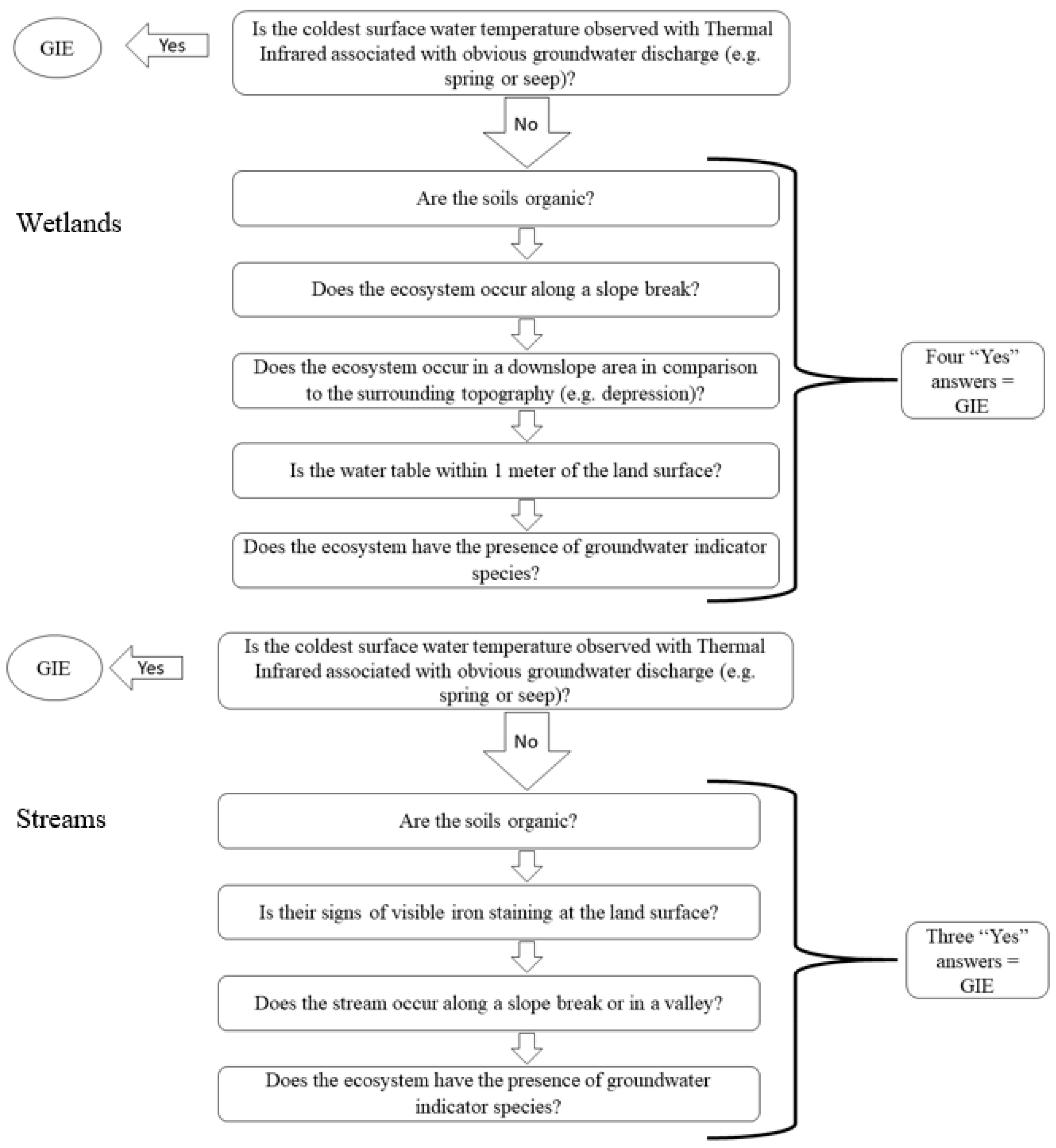
Figure 2. Decision tree for rapid assessment surveys for evidence of groundwater-influenced ecosystems (GIE) in wetlands and streams at sites visited in Atlantic Highlands and Mixed Wood Plains EPA Level II Ecoregions of the northeastern United States during 2020–2022 field seasons (June–September).
Water 15 04035 g002
Figure 3. Mixed Wood Plains and Atlantic Highlands EPA Level II Ecoregion Random Forest model variable importance plots. The greater the percent, the greater the contribution of the variable to the overall fit of the model. The left plot indicates the percent increase in mean square error (IncMSE) when the environmental variable is removed from the model. The right plot indicates the increase in node purity (IncNodePurity), estimating the amount of variation in the data explained by each environmental variable. Mixed Wood Plains Ecoregion abbreviations: hydric = hydric soil, surfmat = surface materials, perm_mw = soil permeability, soildwat_mw = soil water holding capacity, landform = landforms, dem = elevation, wetindex= topographic wetness index (TWI), terrain = terrain roughness index, slope_mw = slope, soildep_mw = soil depth, ndvi_mw = Normalized Difference Vegetation Index. Atlantic Highlands Ecoregion abbreviations: hydric = hydric soil, surfmaterials = surface materials, perm_ah = soil permeability, soilwat = soil water holding capacity, landforms_ah = landforms, dem = elevation, wetindex= topographic wetness index (TWI), terrain = terrain roughness index, slope_ah = slope, soildep = soil depth, ndvi_ah = Normalized Difference Vegetation Index.
Water 15 04035 g003
Figure 4. Mixed Wood Plains EPA Level II Ecoregion Maxent model variable importance plot showing percentage contribution of each environmental variable to the overall fit of the model. The greater the percent, the greater the contribution of the variable to the overall fit of the model. hydric = hydric soil, surfmat = surface materials, perm_mw = soil permeability, soildwat_mw = soil water holding capacity, landform = landforms, dem = elevation, wetindex = topographic wetness index (TWI), terrain = terrain roughness index, slope_mw = slope, soildep_mw = soil depth, ndvi_mw = Normalized Difference Vegetation Index.
Water 15 04035 g004
Figure 5. Atlantic Highlands EPA Level II Ecoregion Maxent model variable importance plot showing percentage contribution of each environmental variable to the overall fit of the model. The greater the percent, the greater the contribution of the variable to the overall fit of the model. hydric = hydric soil, soilwat = soil water holding capacity, wetindex = topographic wetness index, dem = elevation, terrain = terrain roughness index, perm_ah = soil permeability, surfmaterials = surface materials, landforms_ah = landforms, slope_ah = slope, soildep = soil depth, ndvi_ah = Normalized Difference Vegetation Index.
Water 15 04035 g005
Figure 6. Atlantic Highlands EPA Level II Ecoregion correlative distribution modeling results for the four modeling methods predicting Groundwater-Influenced Ecosystems (GIEs). Generalized Linear Model (GLM), Generalized Additive Model (GAM), Random Forest, and Maximum Entropy (MaxEnt) predictions span 0 (most unsuitable) to 1 (most suitable).
Water 15 04035 g006
Figure 7. Mixed Wood Plains EPA Level II Ecoregion correlative distribution modeling results for the four modeling methods predicting Groundwater-Influenced Ecosystems (GIEs). Generalized Linear Model (GLM), Generalized Additive Model (GAM), Random Forest, and Maximum Entropy (MaxEnt) predictions span 0 (most unsuitable) to 1 (most suitable).
Water 15 04035 g007
Figure 8. Areas in the Mixed Wood Plains EPA Level II Ecoregion where suitable conditions are predicted for groundwater-influenced ecosystem occurrence ((A) 0.70 threshold; (B) Natural Breaks). Values indicate the number of models in agreement (e.g., 2 = 2 models in agreement). The models in agreement in each pixel are presented with Supplementary Materials, Figure S2.
Water 15 04035 g008
Figure 9. Areas in the Atlantic Highlands EPA Level II Ecoregion where suitable conditions are predicted for groundwater-influenced ecosystem occurrence ((A) 0.70 threshold; (B) Natural Breaks). Values indicate the number of models in agreement (e.g., 2 = 2 models in agreement). The models in agreement with each pixel are presented in Supplementary Materials, Figure S2.
Water 15 04035 g009
Figure 10. Ensembled model predicted suitability for groundwater-influenced ecosystem occurrence (top left frame) and coefficient of variation between the four model predictions in the Atlantic Highlands EPA Level II Ecoregion. Bottom left and right frames correspond to the same geographic areas that had high predicted landscape suitability for GIEs and also had low coefficient of variation values. White areas in the lower frames indicate open water.
Water 15 04035 g010
Figure 11. Ensembled model predicted suitability for groundwater-influenced ecosystem occurrence (top left frame) and coefficient of variation between the four model predictions in the Mixed Wood Plains EPA Level II Ecoregion. Bottom left and right frames correspond to the same geographic areas that had high predicted landscape suitability for GIEs and also had low coefficient of variation values. White areas in the lower frames indicate open water.
Water 15 04035 g011
Figure 12. Ensembled model predicted suitability for groundwater-influenced ecosystem occurrence in the Atlantic Highlands (top) and the Mixed Wood Plains (bottom) EPA Level II Ecoregion.
Water 15 04035 g012
Table 1. Natural community types characterized as having groundwater connections are included in the Natural Heritage Program occurrence datasets based on community type descriptions and in consultation with state Natural Heritage Program biologists 1 for eight states 2 in the northeastern United States (See Figure 1 for mapped locations).
StateNatural Community Type or Vegetative Community
Connecticut Circumneutral Northern White Cedar Swamp
Circumneutral Spring Fen
Medium Fen
Poor Fen
Rich Fen
Sea Level Fen
MaineAtlantic White Cedar Swamp
Black Ash Swamp
Circumneutral Fen
Evergreen Seepage Forest
Hardwood Seepage Forest
Northern White Cedar Swamp
Open Cedar Fen
Pocket Swamp
Riverside Seep
Massachusetts Acidic Graminoid Fen
Acidic Graminoid Fen-Spillway Fen
Acidic Shrub Fen
Alluvial Atlantic White Cedar Swamp
Alluvial Red Maple Swamp
Calcareous Basin Fen
Calcareous Seepage Marsh
Calcareous Sloping Fen
Interdunal Marsh/Swale
Kettlehole Wet Meadow
Red Maple- Black Ash- Bur Oak Swamp
Red Maple- Black Ash- Tamarack Calcareous Seepage Swamp
Red Maple- Black Ash Swamp
Red Maple Swamp
Rich Conifer Swamp
Riverside Seep Community
Sea-Level Fen
New HampshireAcidic Riverside Seep
Alder-lake Sedge Intermediate Fen
Calcareous Riverside Seep
Calcareous Sedge- Moss Fen
Calcareous Sloping Fen System
Circumneutral Hardwood Forest Seep
Forest Seep/Seepage Forest System
Herbaceous Seepage Marsh
Lake Sedge Seepage Marsh
Larch-Mixed Conifer Swamp
Montane Sloping Fen System
Montane/near-Boreal Minerotrophic Peat Swamp System
Northern Hardwood-Black Ash-Conifer Swamp
Northern Hardwood Seepage Forest
Northern White Cedar/Balsam Fir Swamp
Northern White Cedar-Hemlock Swamp
Northern White Cedar Seepage Forest
Patterned Fen System
Red Maple-Black Ash Swamp
Sand Plain Basin Marsh System
Subacid Forest Seep
New YorkCoastal Plain Pond
Coastal Plain Poor Fen
Hemlock-Hardwood Swamp
Marl Fen
Medium Fen
Northern White Cedar Swamp
Pine Barrens Vernal Pond
Red Maple-Tamarack Peat Swamp
Rich Graminoid Fen
Rich Hemlock-Hardwood Peat Swamp
Rich Shrub Fen
Rich Sloping Fen
Sea Level Fen
Sedge Meadow
Spruce-Fir Swamp
PennsylvaniaHemlock-Mixed Hardwood Palustrine Forest
Hemlock-Mixed Hardwood Palustrine Woodland
Red Maple- Black Gum Palustrine Forest
Red Spruce- Mixed Hardwood Palustrine Forest
Red Spruce Palustrine Forest
Elm-Ash- Maple Lake plain Forest
Alder-Leaved Buckthorn-Inland Sedge-Golden Ragwort Shrub Fen
Sedge-Mixed Forb Fen
Golden Saxifrage- Pennsylvania Bitter-cress Spring Run
Golden Saxifrage- Sedge Rich Seep
Serpentine Seep
Skunk-cabbage-Golden Saxifrage Seep
Rhode IslandGraminoid Fen
Red Maple Swamp
Seal Level Fen
Seeps, Springs
VermontCalcareous Red Maple-Tamarack Swamp
Calcareous Riverside Seep
Hemlock-Balsam Fir- Black Ash Seepage Swamp
Intermediate Fen
Northern Hardwood Seepage Forest
Poor Fen
Red Maple-Black Ash Seepage swamp
Rich Fen
Woodland Seep
Notes: 1 Natural Area Program data contacts: Connecticut Department of Environmental Protection, email: [email protected]; Maine Department of Conservations Natural Areas Program, email: [email protected]; Massachusetts Division of Fisheries and Wildlife’s Natural Heritage and Endangered Species Program, email: [email protected]; New Hampshire Division of Forests and Lands Natural Heritage Bureau, Link: https://www.nh.gov/nhdfl/about-us/natural-heritage-bureau.htm, accessed on 1 December 2021; New York DEC Natural Heritage Program, email: [email protected]; Pennsylvania Natural Heritage Program, email: [email protected]; Rhode Island Department of Environmental Management’s Natural Heritage Program, Link: https://dem.ri.gov/natural-resources-bureau, accessed on 1 December 2021; Vermont Fish and Wildlife Department’s Nongame and Natural Heritage Program, Link: https://vtfishandwildlife.com/conserve/conservation-planning/natural-heritage-inventory, accessed on 1 December 2021; 2 Natural Area Program data were not available for New Jersey.
Table 2. Environmental variables used to model suitability for Groundwater-Influenced Ecosystems (GIEs) in the Mixed Wood Plains and Atlantic Highlands EPA Level II Ecoregions of the northeastern United States. Data layer pixel resolution is 30 m for all variables.
Environmental VariablesData SourceData DescriptionData Category
Elevation (dem) https://datagateway.nrcs.usda.gov/, accessed on 1 December 2021National Elevation DatasetTopography
Topographic Wetness Index (TWI)https://datagateway.nrcs.usda.gov/, accessed on 1 December 2021National Elevation Dataset—[46] protocolTopography
Landforms (landform)https://www.sciencebase.gov/catalog/item/5373c501e4b0497061278a4f, accessed on 1 December 2021Physical form of feature of the land surfaceTopography
Slope (slope)https://datagateway.nrcs.usda.gov/, accessed on 1 December 2021Percent slope of the land surface derived from Elevation datasetTopography
Terrain Roughness Index (terrain)https://datagateway.nrcs.usda.gov/, accessed on 1 December 2021National Elevation Dataset—Roughness tool—ArcGISTopography
Surficial Materials (surfmat)https://pubs.usgs.gov/of/2003/of03-275/, accessed on 1 December 2021Map database of the surficial materials in the conterminous United States [47]Geology
Hydric Soils (hydric)https://datagateway.nrcs.usda.gov/, accessed on 1 December 2021Soil Survey Database—Gridded SSURGOGeology
Soil Water Holding Capacityhttp://umassdsl.org/, accessed on 1 December 2021Total volume of water available to plants at field capacity [48]Geology
Soil Depth (soildep)http://umassdsl.org/, accessed on 1 December 2021Measures the depth of soils to resistant layer [48]Geology
Soil Permeability
Normalized Difference Vegetation Index
https://water.usgs.gov/GIS/metadata/usgswrd/XML/ussoils.xml#Metadata_Reference_Information, accessed on 1 December 2021
Landsat 8 NDVI Imagery (https://developers.google.com/earth-engine/datasets/catalog/landsat-8, accessed on 1 December 2021)
Inches of infiltration per hour
Measure of the state of plant health
Geology
Vegetation
Table 3. Environmental variable response estimates for the fitted Generalized Additive Model (GAM) predicting 30 m pixel-scale suitability for occurrence of a Groundwater-Influenced Ecosystem in the EPA Level II Mixed Wood Plains Ecoregion of northeastern United States. ‘*’ denotes a significant relationship indicated by a p-value of <0.05.
Parametric Coefficients:
EstimateStd. Errorz ValuePr(>|z|)Significance
(Intercept)−1.92 × 1021.50 × 10700.99999
surfmat3 11.64 × 107.35 × 10−12.2310.02566*
surfmat292.18 × 108.44 × 10−12.5870.00969*
Approximate significance of smoothed terms:
edf 2Ref. df 3Chi. sqp-valuesignificance
s(elevation)3.2834.05410.2260.03929*
s(hydric soil)5.0415.971135.493<2 × 10⁻¹⁶*
s(TWI) 44.3455.25716.8620.00627*
s(soil water holding capacity)4.6785.74318.5690.00383*
s(soil permeability)2.5393.15836.4729.22 × 10−8*
R-sq.(adj) = 0.292Deviance explained = 45%
UBRE 5 = −0.8056Scale est. = 1n = 8271
Notes: 1 surfmat3:eolian sediments, mostly dune sand, thick; and surfmat29:glaciofluvial ice-contact sediments, mostly sand and gravel, thick; 2 Effective degrees of freedom; 3 Reference degrees of freedom; 4 TWI: topographic wetness index; 5 Un-biased Risk Estimator.
Table 4. Environmental variable response estimates for the fitted Generalized Linear Model (GLM) predicting 30 m pixel-scale suitability for occurrence of a Groundwater-Influenced Ecosystem in the EPA Level II Mixed Wood Plains Ecoregion of northeastern United States. ‘*’ denotes a significant relationship indicated by a p-value of <0.05.
Coefficients:
EstimateStd. Errorz ValuePr(>|z|)Significance
(Intercept)−1.78 × 1011.97 × 103−0.0090.992778
Elevation1.66 × 10−34.80 × 10−43.4710.000518*
Hydric soil1.78 × 10−21.40 × 10−312.742<2.00 × 10⁻¹⁶*
surfmat3 11.59 × 107.16 × 10−12.2140.026845*
surfmat291.92 × 108.31 × 10−12.3130.020729*
Soil permeability8.82 × 10−21.40 × 10−26.3142.72 × 10−10*
Null deviance: 2684.5 on 8270 degrees of freedom
Residual deviance: 1601.9 on 8217 degrees of freedom
AIC 2: 2643.9
Number of Fisher Scoring iterations: 17
Notes: 1 surfmat3:eolian sediments, mostly dune sand, thick; and surfmat29:glaciofluvial ice-contact sediments, mostly sand and gravel, thick; 2 Akaike Information Criterion.
Table 5. Environmental variable response estimates for the fitted Generalized Additive Model (GAM) predicting 30 m pixel-scale suitability for occurrence of a Groundwater-Influenced Ecosystem in the EPA Level II Atlantic Highlands Ecoregion of northeastern United States. ‘*’ denotes a significant relationship indicated by a p-value of <0.05.
Parametric Coefficients:
Approximate significance of smoothed terms:
Edf 1Ref. df 2Chi. sqp-valuesignificance
s(elevation)4.1455.12751.3779.77 × 10−10*
s(hydric soil)6.5437.509130.372<2.00 × 10⁻¹⁶*
s(terrain roughness)1.0021.0034.4730.034661*
s(TWI) 35.3956.38376.1386.00 × 10−14*
s(slope)1.0011.0015.4840.019225*
s(soil depth)6.1947.21629.6120.000141*
s(soil water holding capacity)4.7635.841.1162.49 × 10−7*
s(NDVI) 42.6413.41424.6823.84 × 10−5*
R-sq.(adj) = 0.281Deviance explained = 36.90%
UBRE 5 = −2022.6Scale est. = 1n = 9205
Notes: 1 Effective degrees of freedom; 2 Reference degrees of freedom; 3 TWI: topographic wetness index; 4 NDVI: normalized difference vegetation index; 5 Un-biased Risk Estimator.
Table 6. Environmental variable response estimates for the fitted Generalized Linear Model (GLM) predicting 30 m pixel-scale suitability for occurrence of a Groundwater-Influenced Ecosystem in the EPA Level II Atlantic Highlands Ecoregion. ‘*’ denotes a significant relationship indicated by a p-value of <0.05.
Coefficients:
EstimateStd. Errorz ValuePr(>|z|)Significance
(Intercept)−4.65 × 10−19.58 × 10−1−0.4860.627119
Elevation1.08 × 10−32.65 × 10−44.0664.78 × 10−5*
Hydric soil1.23 × 10−21.02 × 10−312.006<2.00 × 10⁻¹⁶*
surfmaterials32 1−1.14 × 105.61 × 10−1−2.0260.042747*
Terrain roughness9.26 × 10−33.04 × 10−33.0450.002324*
Slope−4.88 × 10−28.54 × 10−3−5.7151.10 × 10−8*
Soil water holding capacity−1.28 × 10−13.65 × 10−2−3.4990.000468*
NDVI 2−5.14 × 107.34 × 10−1−7.0072.44 × 10−12*
Null deviance: 3888.4 on 9204 degrees of freedom
Residual deviance: 2749.1 on 9161 degrees of freedom
AIC 3: 4423.1
Number of Fisher Scoring iterations: 14
Notes: 1 surfmaterials32: colluvial sediments and residual material; 2 NDVI: normalized difference vegetation index; 3 Akaike Information Criterion.
Table 7. Evaluation metrics for the Mixed Wood Plains and Atlantic Highlands EPA Level II Ecoregion models. Area Under the Curve (AUC), True Skill Statistic (TSS), Kappa, Sensitivity, Specificity, and Deviance calculations and interpretations are provided in the text. GAM: Generalized Additive Model; GLM: Generalized Linear Model.
EcoregionModelAUCTSSKappaSensitivitySpecificityDeviance
Mixed Wood Plains EcoregionGAM0.870.620.370.730.890.31
GLM0.870.640.280.820.820.34
Random Forest0.930.730.360.870.860.25
Maxent0.90.650.310.810.840.48
Atlantic Highlands Ecoregion GAM0.850.560.250.840.730.41
GLM0.850.570.290.790.780.44
Random Forest0.90.650.330.860.790.36
Maxent0.880.650.30.890.750.63
Table 8. Amount of area (hectares) predicted by the Generalized Linear Model, Generalized Additive Model, MaxEnt, and Random Forest models to be highly suitable for Groundwater-Influenced Ecosystems using the 0.70 and Natural Breaks thresholds in the EPA Level II Atlantic Highlands and Mixed Wood Plains Ecoregions.
Atlantic Highlands Ecoregion0.70Natural Breaks
Models in agreementHectares (% of ecoregion)Hectares (% of ecoregion)
1865,654 (5.7)674,708 (4.5)
2422,683 (2.8)304,189 (2.02)
3329,426 (2.2)249,430 (1.7)
422,027 (0.2)61,710 (0.4)
Mixed Wood Plains Ecoregion
Models in agreementHectares (% of ecoregion)Hectares (% of ecoregion)
11,135,298 (6.2)837,498 (4.6)
2191,663 (1.1)198,025 (1.1)
3319,445 (1.7)243,666 (1.3)
416,431 (0.1)53,285 (0.3)
Table 9. Area (hectares) within states and EPA Level II Atlantic Highlands and Mixed Wood Plains Ecoregions of northeastern United States predicted by our ensemble models to be suitable for presence of groundwater-influenced ecosystems. See Figure 1 for model extents.
StatePredicted Suitable Area
(Hectares)
Proportion of Ecoregion (%)
Atlantic Highlands Ecoregion
Connecticut

6188

0.04
Maine63850.04
Massachusetts21,4710.14
New Hampshire40,7330.27
New Jersey11540.01
New York33,0240.22
Pennsylvania12,4310.08
Vermont47,5010.31
Total168,8871.11
Mixed Wood Plains Ecoregion
Connecticut18,3350.10
Maine21750.01
Massachusetts58,5280.32
New Hampshire89340.05
New York42,3330.23
Pennsylvania69680.04
Rhode Island96830.05
Vermont66930.04
Total153,6490.84
Table 10. Area (hectares) predicted by the ensemble models to be suitable for Groundwater-Influenced Ecosystems (GIEs) and falling within mapped National Wetland Inventory (NWI) wetland or deep-water habitats within the EPA Level II Atlantic Highlands and Mixed Wood Plains Ecoregions. See Figure 1 for model extents.
Mixed Wood Plains Ecoregion
NWI Wetland TypeNumber of Mapped NWI Wetlands Containing Predicted GIEsHectaresProportion of Predicted Groundwater-Influenced Area in Mapped NWI Wetland Type (%)Proportion of Mapped NWI Wetlands in Ecoregion (%)
Estuarine and Marine Deepwater302480.030.1
Estuarine and Marine Wetland2736275525
Freshwater Emergent Wetland26,42924,5511811
Freshwater Forested/Scrub Wetland2160.015
Freshwater Forested/Shrub Wetland76,959105,145768
Freshwater Pond9074160812
Lake12837120.50.1
Other283900110
Riverine25,722242821
Total142,790138,163 5
Atlantic Highlands Ecoregion
NWI Wetland TypeNumber of mapped NWI wetlands containing predicted GIEsHectaresProportion of predicted groundwater-influenced area in mapped NWI wetland type (%)Proportion of mapped NWI wetlands in Ecoregion (%)
Estuarine and Marine Deepwater1030.000.2
Estuarine and Marine Wetland 1181020.156
Freshwater Emergent Wetland38,20029,8232125
Freshwater Forested/Shrub Wetland94,970102,3157314
Freshwater Pond14,764276225
Lake2505103310.2
Other170360.036
Riverine38,002474533
Total188,639140,819 9
Note: 1 Estuarine and marine wetlands occur along tidally influenced rivers within the Atlantic Highlands Ecoregion.
Disclaimer/Publisher’s Note: The statements, opinions and data contained in all publications are solely those of the individual author(s) and contributor(s) and not of MDPI and/or the editor(s). MDPI and/or the editor(s) disclaim responsibility for any injury to people or property resulting from any ideas, methods, instructions or products referred to in the content.