1. Introduction
In recent years, Earth-observation-based mapping and monitoring of floods has increasingly utilized synthetic aperture radar (SAR) data [
1]. This situation can be attributed to the excellent systematic acquisition capabilities of the Copernicus Sentinel-1 mission [
2]. In the past two years alone, multiple large-scale flood events have been monitored and analyzed in unprecedented detail using SAR-based methods [
3,
4]. These methods must work on time and provide accurate results, giving decision-makers actionable information for disaster relief, recovery, and reconstruction [
5].
Previous studies have demonstrated SAR-based flood mapping workflows to work well, but with some well-known limitations [
6,
7,
8,
9,
10,
11]. Problems arise in areas where SAR data (only) flood retrievals become ambiguous. Examples are other low-backscatter areas, such as radar shadow regions, or no-sensitivity areas like dense vegetation. In some studies, localized parameterizations (e.g., changing thresholds) or more complex methods [
12,
13,
14,
15,
16] address these concerns but are seldom near-real-time (NRT) or globally viable.
Other workflows rely on exclusion masking of these problematic areas [
8,
17]. While masking is a reasonable solution, over-application is a concern and should be minimized. One commonly used masking method that minimizes misclassification of SAR flood lookalikes uses the height above the nearest drainage (HAND) index [
18,
19]. HAND masking, while known to work well in removing false positives based on topography [
8,
20], often affects significant portions of a flood scene, rendering the mapping algorithm futile for these parts. Despite this concern, HAND masking’s simple execution and robust global performance make it an ideal inclusion in operational workflows [
21].
One flood mapping algorithm in operational use for the new Global Flood Monitoring service [
22] of the Copernicus Emergency Management Service (CEMS,
https://emergency.copernicus.eu/, accessed on 14 September 2023) is the TU Wien flood mapping algorithm. This method is based on a probabilistic Bayesian method [
23] that can integrate pre-existing information (from auxiliary sources) to arrive at improved decisions or classifications. However, using other information to form prior probabilities (or
priors for short) is often overlooked in SAR-based flood mapping efforts in favor of non-informed priors [
24]. In doing so, they miss the potential to improve areas where SAR backscatter alone is ambiguous or problematic. With limited studies having shown success [
5,
25] and others presenting evidence to the contrary [
24], a systematic study of priors in Bayesian SAR-based flood mapping is needed.
This study aims to improve the TU Wien flood mapping algorithm. To accomplish this, instead of using it for masking, we leverage the HAND index to derive priors. We introduce a HAND prior probability function, derive globally applicable parameters, and show its performance on flooded and non-flooded cases in six study sites across the globe.
2. Height above the Nearest Drainage as a Prior
2.1. SAR Flood Mapping Using Bayes Inference
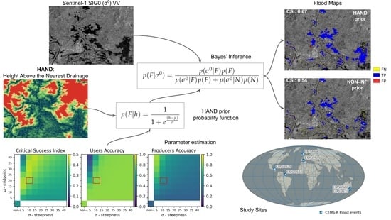
Bayesian classifiers are probabilistic classifiers that apply Bayes’ Theorem. In Earth observation applications, particularly flood mapping applications, these classifiers are usually applied at the pixel level. Pixels are classified as flooded when the probability after inference, or the so-called posterior probability, exceeds a pre-defined threshold (usually 50%). One can calculate the posterior probabilities from Bayes’ inference using:
where
is the conditional probability for a pixel being non-flooded and
for the flooded case, while
and
are the prior probabilities of a pixel being flooded and non-flooded respectively. Most literature has focused on formulating the conditional probability functions, using:
Observed SAR parameters: backscatter intensity [
23,
24], backscatter difference [
26], or coherence [
25];
Probability distribution models: Gaussian [
23,
25,
26,
27] against non-Gaussian [
24];
Dataset used as a reference for flooded probability distribution: scene-based [
24,
25,
27] or historically sampled [
23,
26];
Dataset used as a reference for non-flooded probability distribution: scene-based [
24,
25,
27] against time-series-derived [
23,
26].
In the case of the TU Wien algorithm [
23] tested in this study,
is derived from a harmonic model describing the local VV backscatter, expressed as the expected sigma-naught value (
or SIG0) for a given day of the year.
is estimated from calm water samples, taken at different locations over sea and lakes at times without strong winds.
On the other hand, prior probabilities are often reduced to the non-informative case [
26,
28], i.e., equal chances of being flooded or non-flooded. Giustarini et al. justified this assertion by testing varying prior probability values without significantly affecting the reliability metric of their flood maps [
24]. Further testing priors based on flooded area percentages from reference datasets also did not significantly improve the results in their study. However, their study applied prior values uniformly across their study areas and did not investigate priors that spatially vary.
Reffice et al. discuss the possibilities of such localized priors in their study [
25]. Their study demonstrates a prior probability distribution function from the inverse distance to rivers. Moreover, their subsequent work with a Bayesian network included a piece-wise geomorphic-flooding-index-based function as an auxiliary input [
5]. While both functions offer simple solutions, their approach involves localized optimization of their proposed functions.
2.2. HAND-Based Prior Probability Function
HAND is a hydrological model derived from terrain data such as digital elevation models (DEMs) [
19]. As an index, it is often utilized in SAR-based flood methods to exclude improbable flooded pixels [
29], specifically for low-backscatter pixels above a pre-defined height threshold relative to the nearest drainage level. In machine learning-based flood mapping algorithms, it has also been used as an auxiliary input [
30]. Notably, flood modelers use HAND with synthetic rating curves for rapid inundation mapping [
31,
32,
33], and it has been touted for its performance despite its simplicity.
Our hypothesis is that the HAND index is an ideal candidate prior information in the global operational context because: (1) as there are several (near-) global DEMs openly available, it can be computed globally [
34,
35], (2) it is a simple model (applied the same way everywhere), and (3) it does not require regular updates (since most terrains are primarily stable).
Considering this, we conceptualize a prior probability function that shares HAND’s robustness and simplicity. Thus, only the HAND index is used as an input in our Bayesian inference formulation to estimate the flooded prior probabilities,
, while the non-flooded prior,
, is computed from 1 −
. For
, we propose an exponential function
given as follows:
where
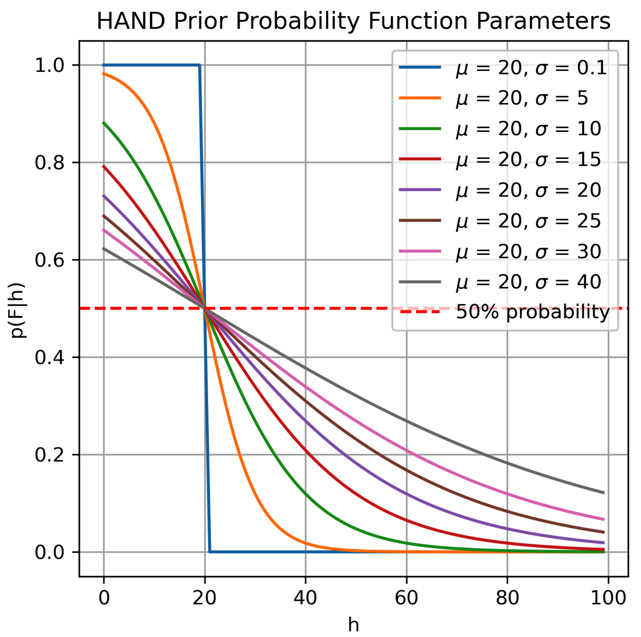
The midpoint () defines the HAND value where the probability indicates a 50% chance of the pixel being labeled as water. In contrast, the steepness parameter () dictates the degree to which the resulting probability changes per increase in HAND value, essentially controlling the function’s characteristic shape. A lower value (e.g., ) results in a function behaving like a step(down) function, while a higher value (e.g., ) leads to an almost linearly decreasing function.
Figure 1 illustrates the response of the proposed function to varying steepness parameter, here centered at
. This exponential formulation models a gentle decrease in probabilities at lower HAND values where flooding is more likely to occur, while having a steeper decline towards the midpoint where floods are less likely to happen.
Similar exponential functions have been proposed by Refice et al. for their distance-to-river function [
25] and Jafarzadegan et al. for their log-normal flood probability function used for HAND-based flood mapping [
31]. The latter reports a similar function being stable during parameter optimization, showing robustness to parameterization, a preferred characteristic for global operations [
36].
3. Materials and Methods
3.1. Study Sites
To test the performance of Bayesian flood mapping with HAND priors, we analyzed flood events and no-flood cases at six test sites covering different geographical regions, climatic conditions, and terrain properties. The details are described in
Section 4.2.
Table 1 shows an overview of these six test sites.
The flood events were identified from available Copernicus Emergency Management Service (CEMS) [
37] rapid mapping activation covering flood events mapped with Sentinel-1 as satellite data input from March to November 2022. This ensured having reference flood extents for our analysis that match our generated flood maps exactly spatially (minimal resolution and sampling effects) and temporally (no time lags).
3.2. Materials
3.2.1. Sentinel-1 Datacube
The Sentinel-1 datacube curated and managed by TU Wien and EODC [
38] serves as the primary data source for the Bayesian flood mapping workflow [
23] employed in this study. This datacube was generated from Sentinel-1 Ground Range Detected (GRD) datasets [
39], which are sampled at a 20 m × 20 m pixel size and tiled at the T3 tiling level (300 km extents) of the Equi7Grid system [
40]. The matching SAR images with the VV polarization band for the six flood events were queried from this datacube. Harmonic parameters were also derived from this datacube [
41] to estimate the day-of-year no-flood reference for the pixel-based flood inference.
3.2.2. Height above the Nearest Drainage
Deriving the HAND index is a reasonably straightforward raster-based methodology using hydrologically conditioned digital elevation models [
19]. While several global HAND datasets are openly available [
35,
42], we computed HAND index datasets from 90 m SRTM [
34] using a Python script with ArcGIS (10.x) ‘Spatial Analyst Tools.tbx’ and ‘Topography Tools 10_2_1.tbx’. This dataset was resampled at a 20 m resolution and tiled to align with the Sentinel-1 datacube.
Locally improving HAND by optimizing the contributing drainage area is recommended [
35]. However, good performance as an exclusion mask with global parameters [
21] has been shown to work for SAR-based flood mapping without such optimization. Thus, no localized optimizations were undertaken.
3.2.3. Reference Flood Extents
Obtaining ground truth data for flood mapping is not always possible [
43]. A reasonable alternative is using existing, manually quality-controlled flood extent maps, such as those made available through CEMS. Using the criteria described in
Section 3.1, CEMS reference vector flood extents and associated ancillary data (e.g., AOI, Hydrology) [
44] were downloaded from
https://emergency.copernicus.eu/ (accessed on 14 September 2023). The downloaded reference datasets were subsequently rasterized, reprojected to the Equi7grid tiles, and masked to match the area of interest (AOI) in preparation for the assessments. To better match the flood maps generated with the CEMS flood reference, we used the same CEMS hydrology dataset (rivers, lakes) as a water mask to differentiate flooding from permanently inundated areas [
45].
3.3. HAND Prior Probability Function Parameter Estimation
First, we determined the globally appropriate midpoint () and steepness () parameters for the HAND prior probability function through the iteration and analysis of the average critical success index (CSI), user’s accuracy (UA), and producer’s accuracy (PA) of all test sites relative to their CEMS counterparts.
CSI, defined by Equation (
3), was used because it is a robust estimator of overall flood map performance [
46]. Furthermore, UA and PA, defined by Equations (
4) and (
5), were also used to discern over- and under-estimation tendencies of the proposed improvement. While no assessment metric is without issues, these metrics were selected to reduce dependence on the size of flood extents [
47]. These metrics are computed from the binary confusion matrix of a classified map versus a reference. All assessment metrics are defined by four binary confusion matrix elements, namely: true positive (TP), true negative (TN), false positive (FP), and false negative (FN).
Given the definition of the midpoint (
), we selected our iteration range based on the published values used as HAND exclusion mask thresholds with typical optimization ranges from 5 to 40 m and selected value ranges from 10 to 20 m [
15,
31,
48]. Value ranges in the same magnitude were tested for the steepness (
) to maintain a reasonable steepness of the resulting function.
For each combination of these two parameters, spatially varying HAND-based prior probabilities were computed for flood map generation. Then, the accuracy metrics (against the CEMS reference) were computed, tabulated, and averaged per parameter combination for all test sites. Finally, the estimated optimal parameters were selected based on the maximization of the three metrics.
3.4. Comparative Performance
Using the determined HAND function, we compared the flood maps generated with non-informed priors and HAND-derived prior probabilities to show their performance in flooded and non-flooded scenarios.
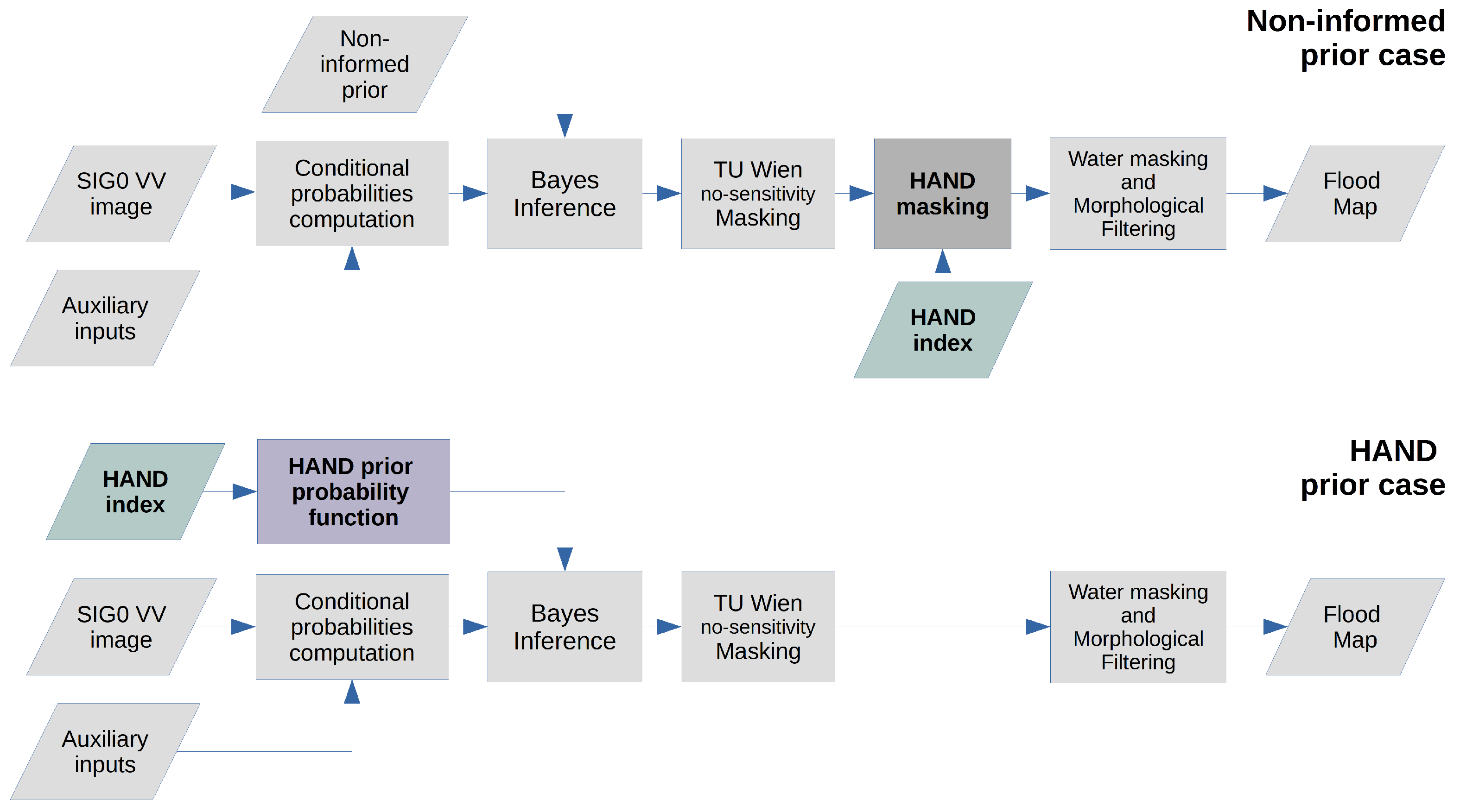
Figure 2 shows the TU Wien flood mapping flowcharts of the two cases, highlighting the difference between the two workflows, consisting of (1) type of input priors and (2) (non-)removal of the HAND mask post-processing step.
As earlier described, raster-based prior probabilities were generated from the HAND dataset using Equation (
2). These prior probabilities were used for the first set of test cases, which we refer to as the HAND prior cases. In contrast, a spatially uniform 0.5 prior probability was used for the second set of test cases for the non-informed prior cases. HAND exclusion masks (using the matching
) were applied as a post-processing step for non-informed prior cases, while this was skipped for the maps computed with HAND prior cases.
Flood maps with both prior cases were generated for flooded-scene scenarios, covering the six flood events. We then computed the (above-mentioned) assessment metrics against the matching pre-processed reference CEMS flood data. After this, we examined the differences in the three metrics between the prior probability cases. Exemplary confusion maps of each site were also created to qualify these differences.
In many cases, flood mapping algorithms are tailor-fitted to work for flooded scenes, which may have a negative effect for monitoring non-flooded scenarios. If an algorithm is applied to a non-flooded image, false positives should not be excessive to give the impression of a scene being flooded. This is important for global monitoring applications where not all results can be manually vetted.
However, in non-flooded scenarios, we lack true positives; thus, the CSI, UA, and PA metrics are not applicable. In their place, we calculated the false positive rate (FPR) [
49] defined by Equation (
6) for maps using both prior cases on exemplary non-flooded images for the same study sites. Here, the binary confusion matrix was generated with a synthetic all-no-flood pixels as reference. In effect, all identified floods are false positives, while non-flooded pixels are true negatives.
The exemplary images were selected to match the same vegetation state as the flooded images. Thus, images approximately one year earlier were identified and matched by orbit to ensure almost identical imaging geometry. These image acquisition dates are noted in
Table 1. While not explicitly screened, no extraneous SAR effects (abnormally high or low backscatter for a scene caused by extremely wet, dry, or windy conditions) were observed in the selected images.
4. Results and Discussions
4.1. Prior Probability Parameterization
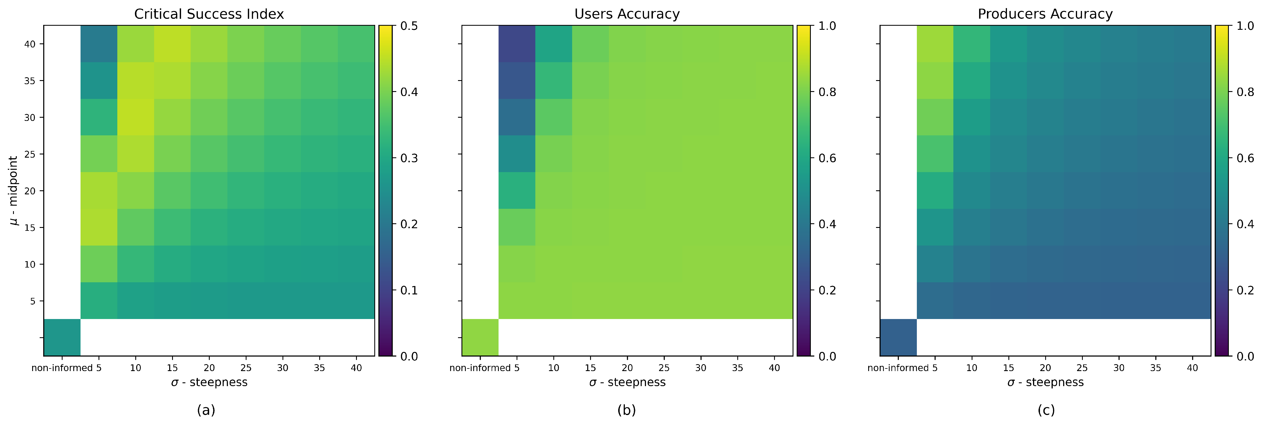
We averaged the CSI, UA, and PA of all six sites across all the parameter iterations to discern an optimal estimate of the function parameters and . As noted earlier, the function response does not significantly change for small parameter changes; hence, for our purpose, the iteration by 5 m of both parameters up to 40 m—leading to 64 combinations—is adequate to arrive at a reasonable estimate of the HAND prior probability function. We plot the metrics for all the combinations for the HAND-based prior function and the non-informed prior case as a reference.
As seen in
Figure 3, panel (a), the best average CSI values were observed with
between 20 and 35 m and
between 5 and 10 m. Moreover, the highest CSI was observed with
m and
m. It should be noted that the CEMS rapid mapping activation uses both the VV and VH bands [
3], while this study focuses on the existing TU Wien workflow using VV polarization only, which could explain the low average CSI values. (We scrutinize these further on a study site basis in
Section 4.2). In terms of thresholding, VH polarization has a slight advantage in mapping complex floods or transition areas, as it more likely exhibits a decrease in backscatter intensity compared to VV polarization, which is more sensitive to complex scattering mechanisms [
50].
As our objective for this study is to improve the algorithm, the absolute CSI values are less important than the observed difference compared with the baseline non-informed prior case. For reference, the overall accuracy values in all test cases for all sites exceeded 87%. They are not presented here for brevity, as the CSI is sufficient to highlight the differences in the overall performance.
On the other hand, the HAND prior parameter combinations and reference non-informed prior results have in general high UA values but show significantly lower values at low values. The PA values, similar to CSI, are not ideal. Most combinations do not significantly change the UA (b). Furthermore, a significant decrease in the UA is observed at between 5 and 10, with a reasonable decrease at less than 25. Lastly, the PA plot in panel (c) shows an increasing value with but a decreasing value with .
Since no combination shows a clear maximum for all three metrics, we can limit the parameter selection to and or and to minimize the decrease in UA while retaining a good CSI and PA improvement. We chose the latter as a conservative estimate for the function parameters.
4.2. Comparative Results HAND Prior
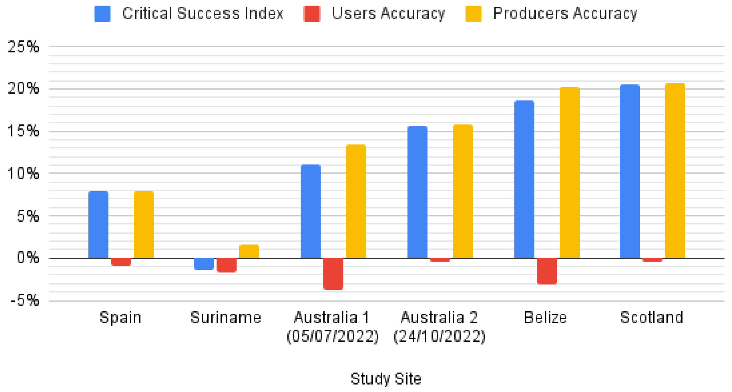
In the following, we describe in detail the performance of this selected parameterization. From
Figure 4, it can be observed that the overall performance on all test sites, except the Suriname test site, has a significantly improved CSI and PA at the expense of a slight decrease in UA.
Interestingly, the study sites that showed the significant improvement in CSI are areas with rolling terrain (Scotland) and low-lying wetland areas (New South Wales, Australia). The improvements are small for urban terrain (Valencia, Spain) and relatively flat areas. This result may be related to the limitation of HAND as a model for relatively flat areas [
32], which in turn is often traced to discrepancies in the source DEM in these areas [
51].
The following sections show confusion maps with water masks overlaid for reference [
45]. We look at the details of the confusion maps of both HAND prior cases and non-informed prior cases to better understand the summarized findings.
4.2.1. Spain
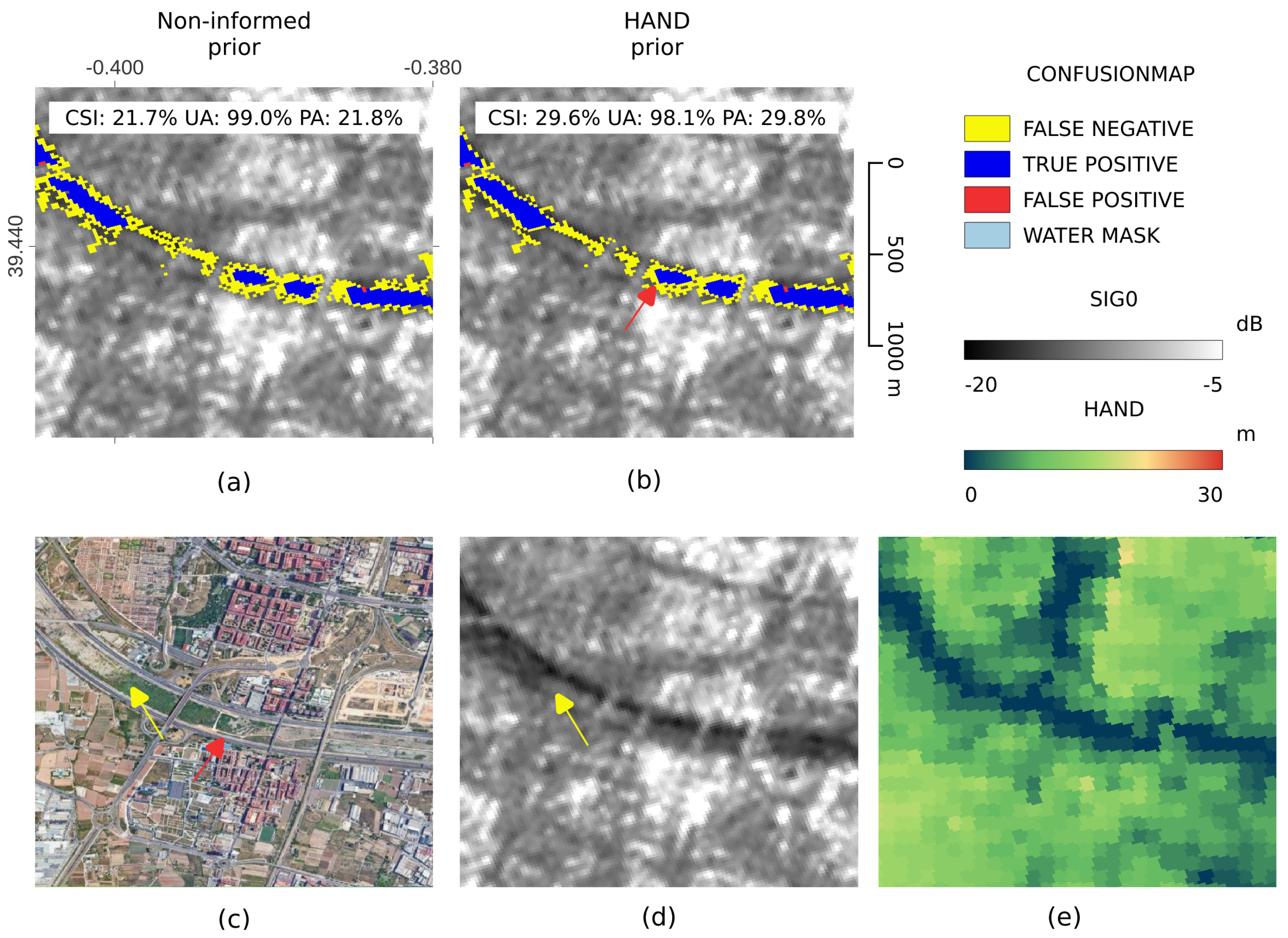
The flood extent from Valencia, Spain, seen in
Figure 5 primarily affected the river Turia and the adjacent green areas. The flooded area visible in the SAR flood maps is centered on its artificial channel. The channel is dotted with varying densities of vegetation. Dense foliage act as a volume scatterer and blocks the impinging signal from reaching the water surface. Thus, sections of the flood along the channel are not visible in the SAR flood maps.
False negatives along the edges of the channel (red arrows) are the most pronounced issue for the flood maps generated, which result in a very low CSI and UA. The channel is characterized by a relatively steep embankment, acting as a transition area and resulting in a complex scattering mechanism where the decrease in backscatter is not as pronounced.
The wider flood extent is better identified by the HAND prior case (b) than the non-informed prior case (a), causing the improvement in PA and CSI. For the most part, the HAND data reflects the low elevations of the channel. However, the resolution of the HAND data (e) is too coarse to cope with the misclassified pixels at the edges. The reference data and flood maps also miss the dense vegetation in the channel (yellow arrows); in this case, even with the highest possible prior probability of being flooded, it is not enough to overturn the non-flood result.
4.2.2. Suriname and Belize
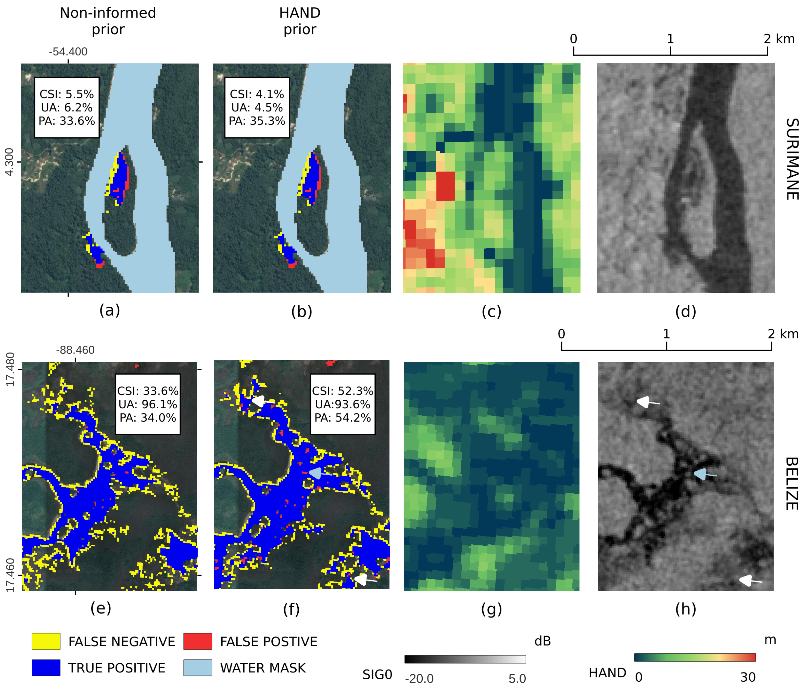
The result for the Suriname test site is shown in the top row of
Figure 6; the area is near Grand Santi, French Guiana. The flood scene indicates overflow along the Marowijne River at the border of Suriname and French Guiana at several small locations. For this site, the HAND prior case does not seem to add value to the original method.
Only minor changes between the HAND prior case (a) and the non-informed prior case (b) were observed at this study site. Since the area is densely vegetated, the quality of the SRTM DEM to represent ground topography is in question [
52,
53]. As observed, most areas have relatively similar and relatively higher HAND values (c) outside the drainage network compared to the other sites, possibly confirming the tree canopy height issue. Thus, the method shows issues due to limitations of the input DEM affecting the HAND prior case performance.
The bottom row of
Figure 6 features the Belize study area, focusing on an area west of Hattieville, Belize. Similar to the Suriname site, most of the area is covered by dense vegetation, but with noticeable patches of sparsely vegetated areas. The confusion maps (e and f) show floods for low-lying clearings. Here, possible flooded vegetation with less considerable decrease in backscatter intensity and flood edges are the most common sources of false negatives in both prior case flood maps. Some of these areas are corrected in the HAND prior case (white arrows). False positives are observed in the HAND prior case not present in the non-informed prior (blue arrow) are pixels with higher backscatter values compared with the surrounding flooded pixels.
4.2.3. Australia
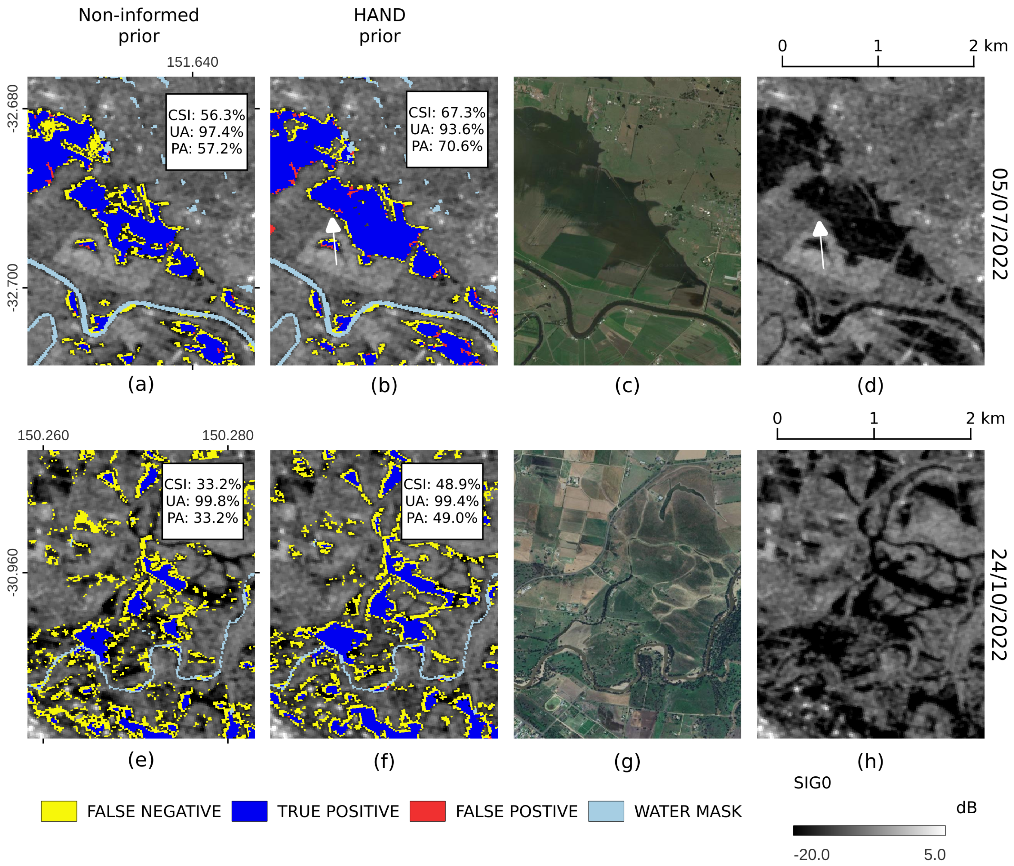
Located in different parts of New South Wales, the 05/07/2022 (Australia 1) and 24/10/2022 (Australia 2) flood events share similar terrain characteristics. Both are located in low-lying areas littered with swamps, creeks, and streams. The 05/07/2022 (Australia 1) event covered the swampy area north of the Hunter River, while the 24/10/2022 (Australia 2) event occurred further inland near the town of Gunnedah and the Namoi River.
Both events cover substantial areas, as seen in
Figure 7. False negatives along the flood borders (or transition zones) are a common issue for both the HAND prior cases (b) and (f) as well as the non-informed prior cases (a) and (e). The HAND prior case showed superior performance in both flood events. Also worth noting are false positives (white arrows) that suggest this area is within the swampy region that is most likely flooded.
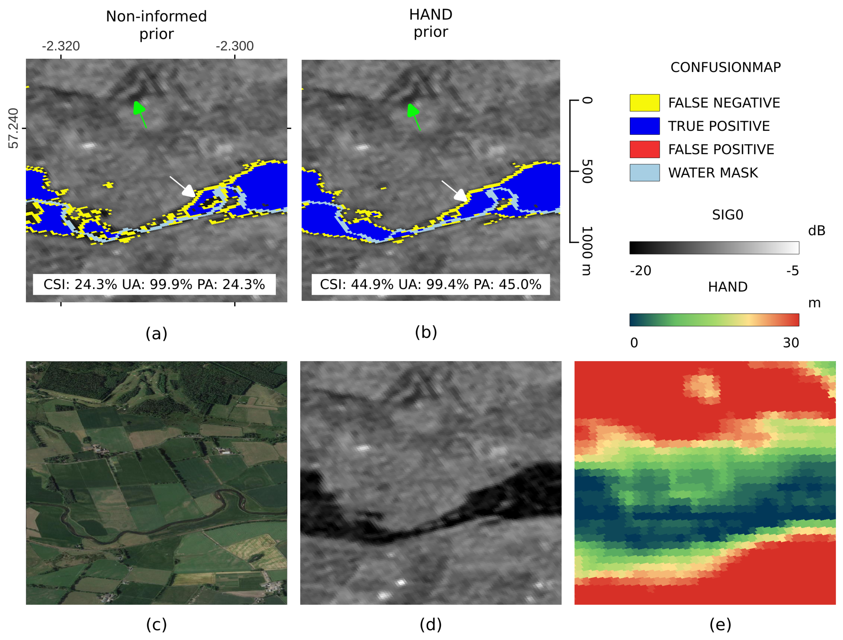
4.2.4. Scotland
The Scotland test case shown in
Figure 8 shows false negative issues around the border areas (white arrows) and masking of dark SAR backscatter pixels at higher elevation (green arrow).
Similar to other test sites, improvements along the flood edges are visible when comparing the non-informed prior case (a) to the HAND prior case (b). These edges or transition zones may contain mixed pixels [
43] and complex scattering mechanisms [
50] that cause a lesser decrease in the SAR (VV polarization) backscatter, which the original algorithm [
23] has issues with and which the HAND priors rectify. Lastly, low-backscatter pixels masked by the HAND mask in the non-informed prior case (b) are labeled as non-flood in the HAND prior case (a).
4.3. No-Flood Conditions
Table 2 shows the FPR calculated from the exemplary non-flooded images. The HAND column shows the FPR of flood maps using the HAND prior probability function, while the No Prior column shows the FPR of the maps with non-informed priors. It can be seen that the Valencia, Spain test site incurs both the largest FPR nominally for both cases and the most significant increase between the two. At the same time, minimal FPR was computed for Suriname. All study sites showed a small increase in FPR with the HAND-based prior, all below 1%.
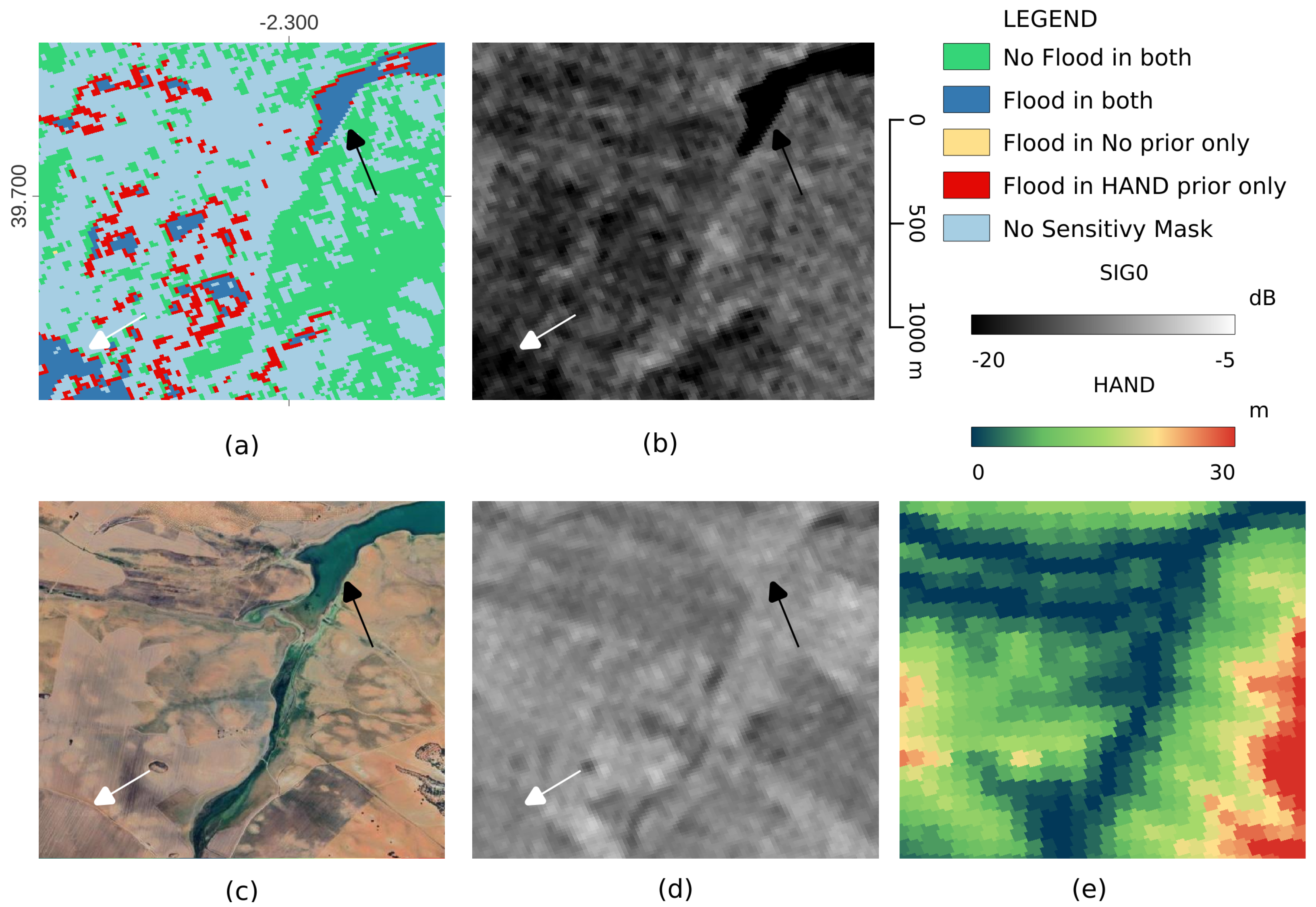
To qualitatively describe the performance of the HAND prior case versus the non-informed prior case in no-flood scenarios, we present the case with the highest FPR (Spain study site), shown in
Figure 9. The zoomed-in area shown is located east of the Alarcon reservoir. It can be observed that the false positives cover (1) reservoir areas that are not normally inundated (black arrows) and (2) low-backscatter areas covering agricultural fields (white arrows). In the former, agricultural fields do not conform with the predicted seasonal backscatter response (see difference between panel d and b), leading to over-estimation—a known issue with the TU Wien algorithm [
23]. At the same time, the latter is a similar case and a common issue in EO flood mapping. Both issues appear to be slightly exacerbated by the HAND prior.
5. Summary and Conclusions
Our results demonstrate a noticeable improvement in the TU Wien flood mapping algorithm by applying a HAND-based prior probability function compared to the baseline non-informed prior. We introduced an exponential function and estimated globally applicable parameters to produce the HAND-based priors. We showed its performance on flooded and non-flooded cases in six study sites.
Concerning the HAND prior probability function, we have not found an optimum for its parameters, as the observed improvement in CSI and PA comes at the cost of UA. Thus, it is prudent to select a conservative estimate for the HAND prior probability function parameters that does not severely impact UA.
While empirically derived, the midpoint at 20m agrees with the assumption that this value should be within the usual range of HAND threshold values. On the other hand, lower steepness values proved to be useful, with 10m working well with the midpoints tested. Further parameter optimization could still improve flood mapping with HAND-based priors. However, given the close responses of the function to changes in parameters, we find the estimated parameters already suitable.
The HAND prior probability function introduced and tested here showed a promising performance. Applying the HAND-based priors decreases false negatives at the expense of a slight increase in false positives. In this regard, we observed less improvement in relatively flat areas than in areas with rolling terrain and low-lying areas. At the same time, we observed instances of similar masking effects when using the HAND prior probability function, thus removing the dependence on HAND masking.
In terms of reducing false negatives, flooded areas with a lesser decrease in backscatter intensities benefit from the HAND prior probabilities. The most commonly observed occurrences of such areas are (1) floods in sparsely vegetated areas and (2) flood boundary or transition regions.
On the other hand, added false positive areas are typically found in low-lying areas with a minimal adverse effect of not masking at higher HAND values. Noting that the CEMS reference flood maps used were also delineated from the same Sentinel-1 images, we observed that some labeled false positives from the HAND prior test cases are most likely true positives that the CEMS rapid mapping method misclassified. On this point, we recommend further testing with independently sourced reference data.
For the no-flood scenarios, a slight increase in the false positive rates was observed for all six study sites tested. This test showed a reasonable performance, with no more than a 1% increase in FPR rates. We observe that the HAND prior slightly exacerbates existing issues with deviations from the expected seasonal backscatter response. Nevertheless, it should be pointed out that no extreme events (very dry or wet conditions) were captured in the six sites tested. As certain extreme events result in low-backscatter signals that lead to wholesale false positives, testing the performance of the HAND prior probabilities in such conditions is recommended.
To conclude, our flood mapping with HAND-based priors demonstrated improvements by decreasing false negatives at low HAND values and preventing false positives at high HAND values. The latter implies that we removed the need for an independent pre- or post-processing HAND mask. However, the improved algorithm has drawbacks: a slight increase in false positive rates and noted limitations for densely vegetated areas. We showed the suitability of applying a single parameterization to the six test sites, suggesting the feasible application of such priors to the TU Wien flood mapping algorithm at a global scale. With its simple formulation and ubiquitous input, this prior formulation could potentially benefit other Bayesian or probabilistic flood mapping workflows.
Author Contributions
Conceptualization, M.E.T. and W.W.; methodology, M.E.T. and W.W.; software, M.E.T. and F.R.; validation, M.E.T.; formal analysis, M.E.T.; investigation, M.E.T.; data curation, M.E.T.; writing—original draft preparation, M.E.T.; writing—review and editing, all authors; visualization, M.E.T.; supervision, B.B.-M. and W.W. All authors have read and agreed to the published version of the manuscript.
Funding
This research was performed with the support of the Engineering Research and Development for Technology Program of the Philippine Department of Science and Technology, the project “S1Floods.AT” (Grant no. BW000028378) founded by the Austrian Rsearch Promotion Agency (FFG), and the project “Provision of an Automated, Global, Satellite-based Flood Monitoring Product for the Copernicus Emergency Management Service” (GFM), Contract No. 939866-IPR-2020 for the European Commission’s Joint Research Centre (EC-JRC). The authors acknowledge TU Wien Bibliothek for financial support through its Open Access Funding by TU Wien.
Data Availability Statement
Acknowledgments
The computational results presented have been achieved using inter alia the Vienna Scientific Cluster (VSC). The authors acknowledge Iftikhar Ali for his contributions in processing the HAND dataset. We would further like to thank our colleagues at TU Wien and EODC for supporting us in technical tasks for maintaining the datacube.
Conflicts of Interest
The authors declare no conflict of interest.
Abbreviations
The following abbreviations are used in this manuscript:
| CEMS | Copernicus Emergency Management Service |
| CSI | Critical Success Index |
| DEM | Digital Elevation Model |
| DOY | Day Of Year |
| EODC | Earth Observation Data Centre for Water Resource Monitoring |
| FPR | False Positive Rate |
| GFM | Global Flood Monitoring |
| GRD | Ground Range Detected |
| HAND | Height Above Nearest Drainage |
| PA | Producer’s Accuracy |
| PLIA | Projected Local Incidence Angle |
| UA | User;s Accuracy |
| PDF | Probability Distribution Function |
| NRT | Near-Real-Time |
| SAR | Synthetic Aperture Radar |
| SIG0 | Sigma Nought backscatter coefficient |
References
- Ajmar, A.; Boccardo, P.; Broglia, M.; Kucera, J.; Giulio-Tonolo, F.; Wania, A. Response to Flood Events. In Flood Damage Survey and Assessment; American Geophysical Union (AGU): Washington, DA, USA, 2017; pp. 211–228. [Google Scholar] [CrossRef]
- Nadine, T.; Stephen, C.; Lucia, L.; Jérôme, M.; Stéphanie, B.; Hervé, Y. Exploitation of Sentinel-1 Data for Flood Mapping and Monitoring within the Framework of the Copernicus Emergency Core and Downstream Services. In Proceedings of the IGARSS 2019–2019 IEEE International Geoscience and Remote Sensing Symposium, Yokohama, Japan, 28 July–2 August 2019; pp. 5393–5396. [Google Scholar] [CrossRef]
- Copernicus Sentinel-1 Facilitates Australia’s Flood Extent Delineation—Sentinel Success Stories—Sentinel Online. Available online: https://sentinel.esa.int/web/success-stories/-/copernicus-sentinel-1-facilitates-australia-s-flood-extent-delineation (accessed on 9 March 2023).
- Roth, F.; Bauer-Marschallinger, B.; Tupas, M.E.; Reimer, C.; Salamon, P.; Wagner, W. Sentinel-1-based analysis of the severe flood over Pakistan 2022. Nat. Hazards Earth Syst. Sci. 2023, 23, 3305–3317. [Google Scholar] [CrossRef]
- D’Addabbo, A.; Refice, A.; Pasquariello, G.; Lovergine, F.P.; Capolongo, D.; Manfreda, S. A Bayesian Network for Flood Detection Combining SAR Imagery and Ancillary Data. IEEE Trans. Geosci. Remote Sens. 2016, 54, 3612–3625. [Google Scholar] [CrossRef]
- Pulvirenti, L.; Pierdicca, N.; Chini, M.; Guerriero, L. An algorithm for operational flood mapping from Synthetic Aperture Radar (SAR) data using fuzzy logic. Nat. Hazards Earth Syst. Sci. 2011, 11, 529–540. [Google Scholar] [CrossRef]
- Martinis, S.; Kuenzer, C.; Wendleder, A.; Huth, J.; Twele, A.; Roth, A.; Dech, S. Comparing four operational SAR-based water and flood detection approaches. Int. J. Remote Sens. 2015, 36, 3519–3543. [Google Scholar] [CrossRef]
- Twele, A.; Cao, W.; Plank, S.; Martinis, S. Sentinel-1-based flood mapping: A fully automated processing chain. Int. J. Remote Sens. 2016, 37, 2990–3004. [Google Scholar] [CrossRef]
- Bioresita, F.; Puissant, A.; Stumpf, A.; Malet, J.P. A method for automatic and rapid mapping of water surfaces from Sentinel-1 imagery. Remote Sens. 2018, 10, 217. [Google Scholar] [CrossRef]
- Shen, X.; Anagnostou, E.N.; Allen, G.H.; Robert Brakenridge, G.; Kettner, A.J. Near-real-time non-obstructed flood inundation mapping using synthetic aperture radar. Remote Sens. Environ. 2019, 221, 302–315. [Google Scholar] [CrossRef]
- Wu, X.; Zhang, Z.; Xiong, S.; Zhang, W.; Tang, J.; Li, Z.; An, B.; Li, R. A Near-Real-Time Flood Detection Method Based on Deep Learning and SAR Images. Remote Sens. 2023, 15, 2046. [Google Scholar] [CrossRef]
- Martinis, S.; Plank, S.; Ćwik, K. The use of Sentinel-1 time-series data to improve flood monitoring in arid areas. Remote Sens. 2018, 10, 583. [Google Scholar] [CrossRef]
- Li, Y.; Martinis, S.; Wieland, M. Urban flood mapping with an active self-learning convolutional neural network based on TerraSAR-X intensity and interferometric coherence. Isprs J. Photogramm. Remote Sens. 2019, 152, 178–191. [Google Scholar] [CrossRef]
- Lin, Y.; Yun, S.H.; Bhardwaj, A.; Hill, E. Urban flood detection with Sentinel-1Multi-Temporal Synthetic Aperture Radar (SAR) observations in a Bayesian framework: A case study for Hurricane Matthew. Remote Sens. 2019, 11, 1778. [Google Scholar] [CrossRef]
- Tsyganskaya, V.; Martinis, S.; Marzahn, P. Flood monitoring in vegetated areas using multitemporal Sentinel-1 data: Impact of time series features. Water 2019, 11, 1938. [Google Scholar] [CrossRef]
- Zhang, M.; Chen, F.; Liang, D.; Tian, B.; Yang, A. Use of sentinel-1 grd sar images to delineate flood extent in Pakistan. Sustainability 2020, 12, 5784. [Google Scholar] [CrossRef]
- Zhao, J.; Pelich, R.; Hostache, R.; Matgen, P.; Cao, S.; Wagner, W.; Chini, M. Deriving exclusion maps from C-band SAR time-series in support of floodwater mapping. Remote Sens. Environ. 2021, 265, 112668. [Google Scholar] [CrossRef]
- Rennó, C.D.; Nobre, A.D.; Cuartas, L.A.; Soares, J.V.; Hodnett, M.G.; Tomasella, J.; Waterloo, M.J. HAND, a new terrain descriptor using SRTM-DEM: Mapping terra-firme rainforest environments in Amazonia. Remote Sens. Environ. 2008, 112, 3469–3481. [Google Scholar] [CrossRef]
- Nobre, A.D.; Cuartas, L.A.; Hodnett, M.; Rennó, C.D.; Rodrigues, G.; Silveira, A.; Waterloo, M.; Saleska, S. Height Above the Nearest Drainage – a hydrologically relevant new terrain model. J. Hydrol. 2011, 404, 13–29. [Google Scholar] [CrossRef]
- Huang, C.; Nguyen, B.D.; Zhang, S.; Cao, S.; Wagner, W. A Comparison of Terrain Indices toward Their Ability in Assisting Surface Water Mapping from Sentinel-1 Data. Isprs Int. J. Geo-Inf. 2017, 6, 140. [Google Scholar] [CrossRef]
- Chow, C.; Twele, A.; Martinis, S. An assessment of the Height Above Nearest Drainage terrain descriptor for the thematic enhancement of automatic SAR-based flood monitoring services. In Proceedings of the Remote Sensing for Agriculture, Ecosystems, and Hydrology XVIII, SPIE, Ediburgh, UK, 26–29 September 2016; Volume 9998, pp. 71–81. [Google Scholar] [CrossRef]
- Salamon, P.; Mctlormick, N.; Reimer, C.; Clarke, T.; Bauer-Marschallinger, B.; Wagner, W.; Martinis, S.; Chow, C.; Böhnke, C.; Matgen, P.; et al. The New, Systematic Global Flood Monitoring Product of the Copernicus Emergency Management Service. In Proceedings of the 2021 IEEE International Geoscience and Remote Sensing Symposium IGARSS, Brussels, Belgium, 11–16 July 2021; pp. 1053–1056. [Google Scholar] [CrossRef]
- Bauer-Marschallinger, B.; Cao, S.; Tupas, M.E.; Roth, F.; Navacchi, C.; Melzer, T.; Freeman, V.; Wagner, W. Satellite-Based Flood Mapping through Bayesian Inference from a Sentinel-1 SAR Datacube. Remote Sens. 2022, 14, 3673. [Google Scholar] [CrossRef]
- Giustarini, L.; Hostache, R.; Kavetski, D.; Chini, M.; Corato, G.; Schlaffer, S.; Matgen, P. Probabilistic Flood Mapping Using Synthetic Aperture Radar Data. IEEE Trans. Geosci. Remote Sens. 2016, 54, 6958–6969. [Google Scholar] [CrossRef]
- Refice, A.; Capolongo, D.; Pasquariello, G.; D’Addabbo, A.; Bovenga, F.; Nutricato, R.; Lovergine, F.P.; Pietranera, L. SAR and InSAR for Flood Monitoring: Examples With COSMO-SkyMed Data. IEEE J. Sel. Top. Appl. Earth Obs. Remote Sens. 2014, 7, 2711–2722. [Google Scholar] [CrossRef]
- Schlaffer, S.; Chini, M.; Giustarini, L.; Matgen, P. Probabilistic mapping of flood-induced backscatter changes in SAR time series. Int. J. Appl. Earth Obs. Geoinf. 2017, 56, 77–87. [Google Scholar] [CrossRef]
- Sherpa, S.F.; Shirzaei, M.; Ojha, C.; Werth, S.; Hostache, R. Probabilistic Mapping of August 2018 Flood of Kerala, India, Using Space-Borne Synthetic Aperture Radar. IEEE J. Sel. Top. Appl. Earth Obs. Remote Sens. 2020, 13, 896–913. [Google Scholar] [CrossRef]
- Westerhoff, R.S.; Kleuskens, M.P.H.; Winsemius, H.C.; Huizinga, H.J.; Brakenridge, G.R.; Bishop, C. Automated global water mapping based on wide-swath orbital synthetic-aperture radar. Hydrol. Earth Syst. Sci. 2013, 17, 651–663. [Google Scholar] [CrossRef]
- Pelich, R.; Chini, M.; Hostache, R.; Matgen, P.; Pulvirenti, L.; Pierdicca, N. Mapping Floods in Urban Areas from Dual-Polarization InSAR Coherence Data. IEEE Geosci. Remote Sens. Lett. 2022, 19. [Google Scholar] [CrossRef]
- Li, Z.; Demir, I. U-net-based semantic classification for flood extent extraction using SAR imagery and GEE platform: A case study for 2019 central US flooding. Sci. Total. Environ. 2023, 869, 161757. [Google Scholar] [CrossRef]
- Jafarzadegan, K.; Merwade, V. Probabilistic floodplain mapping using HAND-based statistical approach. Geomorphology 2019, 324, 48–61. [Google Scholar] [CrossRef]
- Godbout, L.; Zheng, J.Y.; Dey, S.; Eyelade, D.; Maidment, D.; Passalacqua, P. Error Assessment for Height Above the Nearest Drainage Inundation Mapping. J. Am. Water Resour. Assoc. 2019, 55, 952–963. [Google Scholar] [CrossRef]
- Li, Z.; Duque, F.Q.; Grout, T.; Bates, B.; Demir, I. Comparative analysis of performance and mechanisms of flood inundation map generation using Height Above Nearest Drainage. Environ. Model. Softw. 2023, 159, 105565. [Google Scholar] [CrossRef]
- Farr, T.G.; Rosen, P.A.; Caro, E.; Crippen, R.; Duren, R.; Hensley, S.; Kobrick, M.; Paller, M.; Rodriguez, E.; Roth, L.; et al. The Shuttle Radar Topography Mission. Rev. Geophys. 2007, 45. [Google Scholar] [CrossRef]
- Yamazaki, D.; Ikeshima, D.; Sosa, J.; Bates, P.D.; Allen, G.H.; Pavelsky, T.M. MERIT Hydro: A High-Resolution Global Hydrography Map Based on Latest Topography Dataset. Water Resour. Res. 2019, 55, 5053–5073. [Google Scholar] [CrossRef]
- Tupas, M.E.; Roth, F.; Bauer-Marschallinger, B.; Wagner, W. An Intercomparison of Sentinel-1 Based Change Detection Algorithms for Flood Mapping. Remote Sens. 2023, 15, 1200. [Google Scholar] [CrossRef]
- Wania, A.; Joubert-Boitat, I.; Dottori, F.; Kalas, M.; Salamon, P. Increasing Timeliness of Satellite-Based Flood Mapping Using Early Warning Systems in the Copernicus Emergency Management Service. Remote Sens. 2021, 13, 2114. [Google Scholar] [CrossRef]
- Wagner, W.; Bauer-Marschallinger, B.; Navacchi, C.; Reuß, F.; Cao, S.; Reimer, C.; Schramm, M.; Briese, C. A Sentinel-1 Backscatter Datacube for Global Land Monitoring Applications. Remote Sens. 2021, 13, 4622. [Google Scholar] [CrossRef]
- Torres, R.; Snoeij, P.; Geudtner, D.; Bibby, D.; Davidson, M.; Attema, E.; Potin, P.; Rommen, B.; Floury, N.; Brown, M.; et al. GMES Sentinel-1 mission. Remote Sens. Environ. 2012, 120, 9–24. [Google Scholar] [CrossRef]
- Bauer-Marschallinger, B.; Sabel, D.; Wagner, W. Optimisation of global grids for high-resolution remote sensing data. Comput. Geosci. 2014, 72, 84–93. [Google Scholar] [CrossRef]
- Tupas, M.; Navacchi, C.; Roth, F.; Bauer-Marschallinger, B.; Reuß, F.; Wagner, W. Computing Global Harmonic Parameters For Flood Mapping Using Tu Wien’S Sar Datacube Software Stack. Int. Arch. Photogramm. Remote Sens. Spat. Inf. Sci. 2022, 48, 495–502. [Google Scholar] [CrossRef]
- Donchyts, G.; Winsemius, H.; Schellekens, J.; Erickson, T.; Gao, H.; Savenije, H.; van de Giesen, N. Global 30m Height Above the Nearest Drainage. In Proceedings of the Geophysical Research Abstracts, EGU2016-17445-3, 2016, EGU General Assembly, Vienna, Austria, 17–22 April 2016; Volume 18. [Google Scholar] [CrossRef]
- Gstaiger, V.; Huth, J.; Gebhardt, S.; Wehrmann, T.; Kuenzer, C. Multi-sensoral and automated derivation of inundated areas using TerraSAR-X and ENVISAT ASAR data. Int. J. Remote Sens. 2012, 33, 7291–7304. [Google Scholar] [CrossRef]
- Joubert-Boitat, I.; Wania, A.; Dalmasso, S. Manual for CEMS-Rapid Mapping Products; EUR 30370 EN; Publications Office of the European Union: Ispra, Italy, 2020; ISBN 978-92-76-21683-4. [Google Scholar] [CrossRef]
- Wieland, M.; Martinis, S. A Modular Processing Chain for Automated Flood Monitoring from Multi-Spectral Satellite Data. Remote Sens. 2019, 11, 2330. [Google Scholar] [CrossRef]
- Landuyt, L.; Wesemael, A.V.; Schumann, G.J.; Hostache, R.; Verhoest, N.E.C.; Coillie, F.M.B.V. Flood Mapping Based on Synthetic Aperture Radar: An Assessment of Established Approaches. IEEE Trans. Geosci. Remote Sens. 2019, 57, 722–739. [Google Scholar] [CrossRef]
- Stephens, E.; Schumann, G.; Bates, P. Problems with binary pattern measures for flood model evaluation. Hydrol. Process. 2014, 28, 4928–4937. [Google Scholar] [CrossRef]
- Pelich, R.; Chini, M.; Hostache, R.; Matgen, P.; Delgado, J.M.; Sabatino, G. Towards a global flood frequency map from SAR data. In Proceedings of the 2017 IEEE International Geoscience and Remote Sensing Symposium (IGARSS), Fort Worth, TX, USA, 23–28 July 2017; pp. 4024–4027. [Google Scholar] [CrossRef]
- Barsi, Á.; Kugler, Z.; László, I.; Szabó, G.; Abdulmutalib, H.M. Accuracy Dimensions in remote sensing. Int. Arch. Photogramm. Remote Sens. Spat. Inf. Sci. 2018, XLII-3, 61–67. [Google Scholar] [CrossRef]
- Horritt, M.S.; Mason, D.C.; Cobby, D.M.; Davenport, I.J.; Bates, P.D. Waterline mapping in flooded vegetation from airborne SAR imagery. Remote Sens. Environ. 2003, 85, 271–281. [Google Scholar] [CrossRef]
- Garousi-Nejad, I.; Tarboton, D.G.; Aboutalebi, M.; Torres-Rua, A.F. Terrain Analysis Enhancements to the Height Above Nearest Drainage Flood Inundation Mapping Method. Water Resour. Res. 2019, 55, 7983–8009. [Google Scholar] [CrossRef]
- Rabus, B.; Eineder, M.; Roth, A.; Bamler, R. The shuttle radar topography mission—A new class of digital elevation models acquired by spaceborne radar. Isprs J. Photogramm. Remote Sens. 2003, 57, 241–262. [Google Scholar] [CrossRef]
- Li, Y.; Fu, H.; Zhu, J.; Wu, K.; Yang, P.; Wang, L.; Gao, S. A Method for SRTM DEM Elevation Error Correction in Forested Areas Using ICESat-2 Data and Vegetation Classification Data. Remote Sens. 2022, 14, 3380. [Google Scholar] [CrossRef]
Figure 1.
HAND prior probability function response to varying steepness () at midpoint () = 20. Y-axis indicates the probability p(F|h). X-axis indicates the HAND values (h).
Figure 1.
HAND prior probability function response to varying steepness () at midpoint () = 20. Y-axis indicates the probability p(F|h). X-axis indicates the HAND values (h).
Figure 2.
Simplified TU Wien flood mapping flowcharts. Non-informed prior probability case (above). HAND prior probability case (below). Details of the other auxiliary inputs and the TU Wien no-sensitivity and probability distribution-based masking workflow are detailed in the work of Bauer-Maschallinger et al. [
23].
Figure 3.
The average comparative metrics of the study sites versus the prior probability function parameterizations. (a) Average critical success index, (b) average user’s accuracy, and (c) average producer’s accuracy. Y-axis indicates the midpoint (). X-axis indicates the steepness (). The lower left panel shows the non-informed prior case for reference.
Figure 4.
Differences between the comparative metrics. HAND prior case minus non-informed prior case.
Figure 4.
Differences between the comparative metrics. HAND prior case minus non-informed prior case.
Figure 5.
Confusion map of a portion of the Spain study site. Top row: confusion maps for non-informed prior case (a) and HAND prior case (b). Bottom row: true color Google satellite map (c), SIG0 backscatter intensity at VV polarization (d), and HAND index map (e).
Figure 5.
Confusion map of a portion of the Spain study site. Top row: confusion maps for non-informed prior case (a) and HAND prior case (b). Bottom row: true color Google satellite map (c), SIG0 backscatter intensity at VV polarization (d), and HAND index map (e).
Figure 6.
Confusion map of a portion of the Suriname and Belize study sites. Top row: Confusion maps for the Suriname study site overlaid on Google satellite map for non-informed prior case (a) and HAND prior case (b); HAND index map (c) and SIG0 backscatter intensity at VV polarization (d). Bottom row: Confusion maps for the Belize study site overlaid on Google satellite map for non-informed case (e) and HAND prior prior case (f); HAND index map (g) and SIG0 backscatter intensity at VV polarization (h).
Figure 7.
Confusion map of a portion of the New South Wales, Australia study sites. Top row: Confusion maps for the 05/07/2022 (Australia 1) flood event overlaid on SIG0 backscatter intensity at VV polarization for non-informed prior case (a) and HAND prior case (b); Google satellite map (c) and SIG0 backscatter intensity at VV polarization (d). Bottom row: Confusion maps for the 24/10/2022 (Australia 2) flood event overlaid on SIG0 backscatter intensity at VV polarization for non-informed prior case (e) and HAND prior case (f); Google satellite map (g) and SIG0 backscatter intensity at VV polarization (h).
Figure 8.
Confusion map of a portion of the Scotland study site. Top row: non-informed confusion maps for prior case (a) and HAND prior case (b). Bottom row: True color Google satellite map (c), SIG0 backscatter intensity at VV polarization (d), and HAND index map (e).
Figure 8.
Confusion map of a portion of the Scotland study site. Top row: non-informed confusion maps for prior case (a) and HAND prior case (b). Bottom row: True color Google satellite map (c), SIG0 backscatter intensity at VV polarization (d), and HAND index map (e).
Figure 9.
Confusion map of a non-flooded scenario in a portion of the Spain study site. Top row: difference map between the non-informed prior case and HAND prior case (a). SIG0 backscatter intensity at VV polarization on 2023-03-21 (b). Bottom row: true color Google satellite map (c), day-of-year estimated SIG0 backscatter intensity at VV polarization from the harmonic model (d), and HAND index map (e).
Table 1.
Test Sites and Matching CEMS Activations with Flood Event Dates and No-Flood Dates.
Table 1.
Test Sites and Matching CEMS Activations with Flood Event Dates and No-Flood Dates.
| CEMS Activation | Type | Location | Flood Event Date | No-Flood Date |
|---|
| EMSR569 | Flood | Valencia, Spain | 22/03/2022 | 21/03/2021 |
| EMSR577 | Flood | Suriname | 16/06/2022 | 09/06/2021 |
| EMSR586 | Flood | New South Wales, Australia | 05/07/2022 | 16/06/2021 |
| EMSR637 | Flood | New South Wales, Australia | 24/10/2022 | 17/10/2021 |
| EMSR639 | Flood | Belize | 03/11/2022 | 27/10/2021 |
| EMSR640 | Flood | Scotland, United Kingdom | 20/11/2022 | 25/11/2021 |
Table 2.
False Positive Rates for No-Flood Cases.
Table 2.
False Positive Rates for No-Flood Cases.
| Location | No Prior | HAND Prior | Difference |
|---|
| Spain | 1.50% | 2.43% | 0.92% |
| Suriname | 0.00% | 0.00% | 0.00% |
| Australia 1 | 0.03% | 0.12% | 0.09% |
| Australia 2 | 0.07% | 0.66% | 0.59% |
| Belize | 0.04% | 0.20% | 0.16% |
| Scotland | 0.14% | 0.14% | 0.00% |
| average | 0.30% | 0.59% | 0.29% |
| Disclaimer/Publisher’s Note: The statements, opinions and data contained in all publications are solely those of the individual author(s) and contributor(s) and not of MDPI and/or the editor(s). MDPI and/or the editor(s) disclaim responsibility for any injury to people or property resulting from any ideas, methods, instructions or products referred to in the content. |
© 2023 by the authors. Licensee MDPI, Basel, Switzerland. This article is an open access article distributed under the terms and conditions of the Creative Commons Attribution (CC BY) license (https://creativecommons.org/licenses/by/4.0/).


