Evaluation of Empirical Equations and Machine Learning Models for Daily Reference Evapotranspiration Prediction Using Public Weather Forecasts

Abstract

Although the studies on model prediction of daily ET_o based on public weather forecasts have been widely used, these studies lack the comparative evaluation of different types of models and do not evaluate the seasonal variation in model prediction of daily ET_o performance; this may result in the selected model not being the best model. In this study, to select the best daily ET_o forecast model for the irrigation season at three stations (Yinchuan, Tongxin, and Guyuan) in different climatic regions in Ningxia, China, the daily ET_os of the three sites calculated using FAO Penman–Monteith equations were used as the reference values. Three empirical equations (temperature Penman–Monteith (PMT) equation, Penman–Monteith forecast (PMF) equation, and Hargreaves–Samani (HS) equation) were calibrated and validated, and four machine learning models (multilayer perceptron (MLP), extreme gradient boosting (XGBoost), light gradient boosting machine (LightGBM), and gradient boosting with categorical features support (CatBoost)) were trained and validated against daily observed meteorological data (1995–2015 and 2016–2019). Based on public weather forecasts and daily observed meteorological data (2020–2021), the three empirical equations (PMT, PMF, and HS) and four machine learning models (MLP, XGBoost, LightGBM, and CatBoost) were compared in terms of their daily ET_o prediction performance. The results showed that the daily ET_o performance of the seven models in the irrigation season with a lead time of 1–7 days predicted by the three research sites decreased in the order of spring, autumn, and summer. PMT was the best model for the irrigation seasons (spring, summer, and autumn) at station YC; PMT and CatBoost with C3 (T_max, T_min, and Wspd) as the inputs were the best models for the spring, autumn irrigation seasons, and summer irrigation seasons at station TX, respectively. PMF, CatBoost with C4 (T_max, T_min) as input, and PMT are the best models for the spring irrigation season, summer irrigation season, and autumn irrigation season at the GY station, respectively. In addition, wind speed (converted from the wind level of the public weather forecast) and sunshine hours (converted from the weather type of the public weather forecast) from the public weather forecast were the main sources of error in predicting the daily ET_o by the models at stations YC and TX(GY), respectively. Empirical equations and machine learning models were used for the prediction of daily ET_o in different climatic zones and evaluated according to the irrigation season to obtain the best ET_o prediction model for the irrigation season at the study stations. This provides a new idea and theoretical basis for realizing water-saving irrigation during crop fertility in other arid and water-scarce climatic zones in China.

1. Introduction

Evapotranspiration is a key link in the surface water cycle and an important basis for crop water demand determination. Evapotranspiration is generally obtained by multiplying the reference evapotranspiration (ET_o) by the crop coefficient. The determination of ET_o is not only a key factor in predicting and estimating crop water demand but also an important requirement for irrigation forecasting and irrigation decision making. Timely and accurate ET_o prediction has a notable reference value for real-time irrigation decision making [1] and is very important for improving the real-time irrigation prediction accuracy, irrigation management level, crop yield, and water conservation [2].

Depending on the adopted method and input data, ET_o prediction methods can be divided into direct and indirect methods [1]. Among the direct methods, time series models, such as autoregressive (AR), moving average (MA), autoregressive moving average (ARMA), and autoregressive integrated moving average (ARIMA) models, have been used to forecast the daily ET_o using historical daily ET_o data calculated from historical daily measured meteorological data [3]; alternatively, machine learning algorithms, such as the multilayer perceptron (MLP), multivariate relevance vector machine (MVRVM) [4], multilayer perceptron–neural network model (MLP-NNM), Kohonen self-organizing feature maps–neural network model (KSOFM-NNM), gene expression programming (GEP) [5], least-squares support vector machine (LSSVM), adaptive neuro-fuzzy inference system (ANFIS), generalized regression neural network (GRNN) [3], deep learning models (long short-term memory (LSTM), one-dimensional convolutional neural network (1D CNN), and a combination of the two previous models (CNN-LSTM)), and traditional machine learning models (artificial neural network (ANN) and random forest (RF)) [6], have been employed to predict the daily ET_o and the daily ET_o at a lead time of 1–7 days using historical data. In these studies, alternatives to time series models have been applied for future ET_o prediction based on historical meteorological data and ET_o calculated with historical meteorological data. In general, machine learning models using ET_o data computed from historical meteorological data outperform those directly using historical meteorological data [3]. In addition, combined machine learning models, such as the fruit fly optimized GRNN model [7] and autoencoder–decoder bidirectional LSTM (AED-BiLSTM) [8], can predict ET_o more accurately than a single machine learning model (GRNN, XGBoost). However, in all these studies, so-called ET_o forecast data generated from long-term historical meteorological data were used, and since the short-term daily ET_o is mainly governed by weather conditions, direct methods may not be applicable [9,10,11].

In the indirect method, ET_o can be calculated using weather variables predicted via numerical weather prediction (NWP) or public weather forecasts, such as those obtained using the Food and Agriculture Organization (FAO)-56 Penman–Monteith (PM) equation [1,12,13,14,15,16], the Hargreaves–Samani (HS) and Priestley (PT) equations [12], or multivariate time series models [17], and the numerical weather forecasts output by forecast systems or models (COSMO, Australian Community Climate and Earth System Simulator–Global (ACCESS-G), Global Ensemble Forecast System (GEFS) model, European Centre for Medium-Range Weather Forecasts (EC), National Centers for Environmental Prediction Global Forecast System (NCEP), and United Kingdom Meteorological Office (MO) forecasts) can be used to predict the daily ET_o, weekly ET_o, and daily ET_o with a lead time of 1–16 days. Although NWP can generate forecasts of the full range of meteorological variables needed by the FAO-56 PM equation and can be used for ET_o prediction, NWP data are not available to the public in some developing countries. For example, the numerical forecast products of the China Meteorological Data Network are only available to registered users for education and research purposes, while numerical forecast products require expert downscaling and bias correction [16] or postprocessing methods [14] to improve their reliability.

In China, the public can easily access free public weather forecasts up to 40 days in advance in real time from China Weather (http://www.weather.com.cn (accessed on 31 December 2022)). These free public weather forecasts include four variables: maximum temperature, minimum temperature, wind scale, and weather type. Over the past decade, public weather forecasts have been widely used for ET_o prediction. For example, information retrieved from public weather forecasts has been converted into the variables needed to calculate ET_o using the FAO-56 PM equation and subsequently applied in daily ET_o prediction [18,19,20,21]. Given that temperature is the most accurate and only quantitative variable in public weather forecasts, many studies have used only temperature forecast data retrieved from public weather forecasts to predict ET_o. Based on temperature data retrieved from public weather forecasts, the daily ET_o has been predicted using locally calibrated versions of the HS equation [9,22,23], the daily ET_o with a lead time of 1–7 days has been predicted using the monthly calibrated Blaney–Criddle (BC) model [24], and four ANN models (linear regression (LR), probabilistic neural network (PNN), MLP, and generalized feedforward (GFF) models) [10], and the GEP algorithm [2] have been used to predict the daily ET_o with a lead time of 1–7 days at Gaoyou Station in Jiangsu Province of China. The above studies based on the adoption of public weather forecast models for daily ET_o prediction have achieved reasonable results, but there exists no evaluation model to determine the seasonal variation in the daily ET_o prediction performance, and there is a lack of comparative evaluation of machine learning models in daily ET_o prediction based on different input combinations of weather variables retrieved from public weather forecasts. These studies are aimed at a single model in a single region (or multiple regions) of China or a comparative study of similar models in a single region (or multiple regions) of China [11]. The lack of comparative research on different types of models can lead to the inability to identify the best daily ET_o forecast model in a given region.

Recently, three tree models based on boosting algorithms, namely, extreme gradient boosting (XGBoost), light gradient boosting machine (LightGBM), and gradient boosting with categorical features support (CatBoost), have been widely used to estimate the daily ET_o [25,26,27,28,29,30,31,32,33] and monthly ET_o [34]. These studies have shown that the daily ET_o estimated by these three tree models is suitably accurate, with a better performance than that of other models. However, there are no studies on ET_o prediction with these three tree models. Compared with estimating historical daily ET_o by models and historical daily measured weather forecast data, it is more valuable to predict future daily ET_o by models and public weather forecasts because accurate prediction of ET_o is the key to crop water demand prediction and the premise of real-time irrigation prediction, which has important reference value and significance for real-time irrigation decision making.

In this paper, three empirical equations and four machine learning models for predicting daily ET_o using public weather forecasts are evaluated to select the best daily ET_o prediction model for the crop irrigation season in the study area. The objectives of this study were as follows: (1) In model assessment based on public weather forecasts, the optimal input combinations of the MLP, XGBoost, LightGBM, and CatBoost machine learning models were determined to obtain the best daily ET_o prediction performance. (2) Three empirical equations (PMT, PMF, and HS) and four machine learning models (MLP, XGBoost, LightGBM, and CatBoost) were compared by determining the seasonal variation in the daily ET_o prediction performance, and the best daily ET_o prediction model was recommended for all four seasons at various research sites in three climate zones. The main error sources of daily ET_o predicted by the PMF equation and four machine learning models were analyzed.

2. Materials and Methodology

2.1. Study Area and Data Collection

2.1.1. Study Area

Ningxia is located deep inland and exhibits typical continental climate characteristics. In China’s climate division, according to the Kottek classification [35], the southern part of Guyuan city (southern mountainous area) belongs to the temperate semihumid zone, the northern part of Yuanzhou District to the Yanchi and Tongxin area (central arid zone) belongs to the temperate semiarid zone, and the northern Yellow River irrigation area belongs to the temperate arid zone. In this study, the Yinchuan station, Tongxin station and Guyuan station in Ningxia, China, were selected. The locations of these three stations are shown in Figure 1.

Table 1. Location characteristics and annual mean values of the meteorological data at each of the three weather stations in this study.

WMO Number	Station	Latitude	Longitude	Elevation	Tmax	Tmin	Tmean	u2	RHmean	Sdun	ETo	Climate Zone
		(N)	(E)	(m)	(°C)	(°C)	(°C)	(m s−1)	(%)	(h)	(mm d−1)
53614	Yinchuan (YC)	38°29′	106°13′	1111.4	17.3	4.8	10.5	1.54	51.11	7.55	3.05	Arid
53810	Tongxin (TX)	36°58′	105°54′	1339.3	17.5	4.2	10.1	2.28	52.47	8.02	3.37	Semiarid
53817	Guyuan (GY)	36°00′	106°16′	1753.0	13.9	2.6	7.7	1.87	58.51	6.95	2.68	Subhumid

lists the longitude, latitude and annual mean values of the meteorological data retrieved from these three stations.

2.1.2. Data Collection

Daily observed meteorological data at the three meteorological stations from 1 January 1995 to 31 December 2021, were obtained from the China Meteorological Data Network (http://data.cma.cn/ (accessed on 31 December 2022)), including the daily maximum temperature (T_max), daily minimum temperature (T_min), average temperature, average relative humidity (RH), sunshine hours (SDun), and average wind speed (Wspd). Daily public weather forecast data 1–7 days in advance from 1 January 2020 to 31 December 2021, at the same sites were collected from the China Weather Network (http://www.weather.com.cn (accessed on 31 December 2022)), including the daily maximum temperature (T_max), daily minimum temperature (T_min), wind scale, and weather type. Daily observed meteorological data from 1 January 1995 to 31 December 2015, were used to calibrate the three empirical equations and train the four machine learning models, and daily observed meteorological data from 1 January 2016 to 31 December 2019 were employed to validate the three empirical equations and four machine learning models. Daily public weather forecast data with a lead time of 1–7 days and daily observed meteorological data from 1 January 2020 to 31 December 2021 were used to test and evaluate the performance of these seven models.

2.2. Methodology

2.2.1. FAO Penman–Monteith (PM) Equation

The daily ET_o calculated using the FAO-56 Penman–Monteith equation [36] recommended by the United Nations Food and Agricultural Organization (FAO) and daily observed meteorological data were used to evaluate the performance of the three empirical equations and four machine learning models to predict ET_o. The FAO-56 PM equation [36] can be expressed as follows:

$${\mathrm{E}\mathrm{T}}_{\mathrm{o}}=\frac{0.408∆\left(R_n-G\right)+\gamma \frac{900}{T+273}{u}_2\left(e_s-e_a\right)}{∆+\gamma \left(1+0.34u_2\right)}$$

(1)

where ET_o is the daily reference evapotranspiration [mm day⁻¹]; R_n is the net radiation at the crop surface [MJ m⁻² day⁻¹]; G is the soil heat flux density [MJ m⁻² day⁻¹] (G may be ignored during the day); T is the mean daily air temperature at the 2 m height [°C]; u₂ is the wind speed at the 2 m height [m s⁻¹]; e_s is the saturation vapor pressure [kPa]; e_a is the actual vapor pressure [kPa]; e_s − e_a is the saturation vapor pressure deficit [kPa]; ∆ is the slope of the vapor pressure curve [kPa °C⁻¹]; and γ is the psychrometric constant [kPa °C⁻¹].

2.2.2. Temperature Penman–Monteith (PMT) Equation

When humidity and radiation data are unavailable, Allen et al. [36] proposed a method for ET_o calculation using only the maximum temperature, minimum temperature, and wind speed at the 2 m height, namely, the PMT method. The main calculation process can be expressed as Equations (2)–(8) [36]. ET_o was predicted by estimating the actual saturated vapor pressure (e_a) using the dew point temperature (T_dew) and solar radiation (R_s) considering the maximum and minimum air temperatures; the wind rating in public weather forecast information was converted into the wind speed according to

Table 2. Beaufort wind scale (GB/T 35227—2017, 2017) [41].

Wind Scale	Designation	u10 (ms−1)
		Range	Average (WSpd)
0	Calm	0.0–0.2	0.0
1	Light	0.3–1.5	1.0
2	Slight	1.6–3.3	2.0
3	Gentle	3.4–5.4	4.0
4	Moderate	5.5–7.9	7.0
5	Fresh	8.0–10.7	9.0
6	Strong wind	10.8–13.8	12.0
7	High wind	13.9–17.1	16.0
8	Gale	17.2–20.7	19.0
9	Strong gale	20.8–24.4	23.0
10	Whole gale	24.5–28.4	26.0
11	Storm	28.5–32.6	31.0
12	Hurricane	32.7–36.9	35.0

. However, Equation (2) was established for T_dew = T_min, and a correction for T_dew is needed in practical applications [36]. Similarly, the adjustment coefficient k_Rs in Equation (4) is an empirical value that differs between interior and coastal regions, and k_Rs must also be corrected [11,37,38,39,40]:

$${\mathrm{e}}_a=e^o\left(T_{min}\right)=0.611\exp \left[\frac{17.27T_{min}}{T_{min}+237.3}\right]$$

(2)

$$\begin{array}{c}{\mathrm{R}}_a=\frac{24\left(60\right)}{\pi }{G}_{sc}{d}_r\left[{\omega }_s\sin \left(\phi \right)\sin \left(\delta \right)+\cos \left(\phi \right)\cos \left(\delta \right)\sin \left({\omega }_s\right)\right]\end{array}$$

(3)

$${\mathrm{R}}_s={\mathrm{k}}_{Rs}\sqrt{\left(T_{max}-T_{min}\right)}{\times R}_a$$

(4)

$${\mathrm{R}}_{so}=\left(a_s+b_s\right)R_a$$

(5)

$${\mathrm{R}}_{ns}=\left(1-\alpha \right)R_s$$

(6)

$${\mathrm{R}}_{nl}=\sigma \left[\frac{{T_{max,K}}^4+{T_{min,K}}^4}{2}\right]\left(0.34-0.14\sqrt{e_a}\right)\left(1.35\frac{R_s}{R_{SO}-0.35}\right)$$

(7)

$${\mathrm{R}}_n=R_{ns}-R_{nl}$$

(8)

where e^o (T_min) is the saturation vapor pressure at the daily minimum temperature [kPa]; R_a is the extraterrestrial radiation [MJ m⁻² day⁻¹]; G_SC is a solar constant = 0.0820 [MJ m⁻² min⁻¹]; d_r is the inverse relative distance between the Earth and Sun; ${\omega }_s$ is the sunset hour angle [rad]; $\phi$ is the latitude [rad]; $\delta$ is the solar declination [rad]; R_s is the solar or shortwave radiation [MJ m⁻² day⁻¹]; T_max and T_min are the daily maximum and minimum air temperatures, respectively [°C]; k_Rs is the adjustment coefficient (0.16..0.19) [°C^−0.5], and at interior locations, k_Rs = 0.16, while at coastal locations, k_Rs = 0.19; z is the station elevation above sea level [m]; R_so is the clear-sky solar radiation [MJ m⁻² day⁻¹]; R_ns is the net solar or shortwave radiation [MJ m⁻² day⁻¹]; α is the albedo or canopy reflection coefficient (α = 0.23); R_nl is the net outgoing longwave radiation [MJ m⁻² day⁻¹]; σ is the Stefan–Boltzmann constant [4.903 × 10⁻⁹ MJ K⁻⁴ m⁻² day⁻¹]; T_max,K is the maximum absolute temperature during the 24-h period [K = °C + 273.16]; and T_min,K is the minimum absolute temperature during the 24-h period [K = °C + 273.16].

2.2.3. Penman–Monteith Forecast (PMF) Equation

The wind scale and weather type in public weather forecast information cannot be directly used for ET_o prediction. Cai et al. [18] proposed an analytical method, namely, the PMF method [11,20,21]. ET_o can be predicted by converting the wind scale into the wind speed according to Table 2, while the weather type can be transformed into the sunshine duration coefficient according to

Table 3. Conversion relationship between the weather type and sunshine duration coefficient.

Weather Type	Sunny	Clear to Overcast	Cloudy	Overcast	Rainy	Snow	Dust	Haze
Coeffient (α)	0.9	0.7	0.5	0.3	0.1	0.1	0.2	0.2

[18,20,42]. Moreover, the solar radiation (R_s) can be calculated using Equations (9)–(11), and the actual saturated vapor pressure (e_a) can be estimated with Equation (2). However, the use of the PMF method requires correction for T_dew [37,38,39,40,42]:

$$\mathrm{N}=\frac{24}{\pi }{\omega }_s$$

(9)

$$\mathrm{n}=\mathsf{\alpha }\mathrm{N}$$

(10)

$${\mathrm{R}}_s=\left(a_s+b_s\frac{n}{N}\right)R_a$$

(11)

where N is the maximum possible duration of sunshine or daylight hours [hour]; n is the predicted sunshine duration [hour]; α is the sunshine duration coefficient; a_s is the regression constant, reflecting the fraction of extraterrestrial radiation reaching the Earth on overcast days (n = 0); and a_s + b_s is the fraction of extraterrestrial radiation reaching the Earth on clear-sky days (n = N). Where no actual solar radiation data are available and no calibration is conducted to obtain improved a_s and b_s parameters, a_s = 0.25 and b_s = 0.50 are recommended [11,18,20,36].

2.2.4. Hargreaves–Samani (HS) Equation

The 1985 HS equation has been widely used in ET_o estimation/prediction [9,11,22,23,37,38,39,40,43,44,45,46,47,48,49]. The HS equation can be expressed as Equation (12), which has been applied in practice with corrections for parameters C and E [9,11,50,51]:

$${\mathrm{E}\mathrm{T}}_{\mathrm{o}}=C{R}_a{\left(T_{max}-T_{min}\right)}^E\left[\frac{T_{max}+T_{min}}{2}+17.8\right]$$

(12)

where ET_o is the daily ET_o calculated by the HS equation [mm day⁻¹]; T_max and T_min are the daily maximum and minimum air temperatures, respectively [°C]; R_a is the extraterrestrial radiation [MJ m⁻² day⁻¹]; and C and E are model parameters with suggested initial values of 0.0023 and 0.5, respectively [50].

2.2.5. Multilayer Perceptron (MLP) with Multiple Hidden Layers

The concept of deep learning was proposed by Hinton et al. [52]; an MLP with multiple hidden layers is a typical deep learning structure. MLPs with one or two hidden layers have been widely used for ET_o estimation/prediction [10,53,54,55,56,57,58]. However, in these studies, the number of neurons in a single hidden layer and the number of hidden layers and neurons in each hidden layer have been determined by trial and error, which can be time consuming and may not always yield the best hyperparametric results.

In this study, the number of hidden layers and the number of neurons in each hidden layer are used as hyperparameters, the activation function of the hidden layer is defined as the rectified linear unit (ReLU) function, the optimization method used by the network is defined as stochastic gradient descent (SGD), and a hyperparameter search can be achieved by using RandomizedSearchCV in sklearn to determine the multilayer perceptron that contains multiple hidden layers.

2.2.6. Extreme Gradient Boosting (XGBoost)

The XGBoost algorithm [59] is an improved implementation of the gradient boosting decision tree (GBDT) algorithm framework. XGBoost uses a levelwise decision tree growth strategy that splits all the leaves at the same level simultaneously (equivalent to a full binary tree), thus performing multithreaded optimization, which is less prone to overfitting. This indiscriminate treatment of leaves at the same level allows XGBoost to apply a presorting algorithm to find the optimal split nodes (branching points) in the tree construction process, but this approach is associated with a significant overhead in both space and time. XGBoost cannot directly manage categorical features but employs preprocessing by various encoding methods, such as token encoding, mean encoding, or unique hot encoding. The XGBoost open source can be obtained from http://xgboost.readthedocs.io (accessed on 31 December 2022).

2.2.7. Light Gradient Boosting Machine (LightGBM)

The LightGBM algorithm [60] is also based on the GBDT algorithm. LightGBM uses a leafwise decision tree growth strategy with depth restrictions to find the model with the highest splitting gain (and generally the largest amount of data) from all the current leaves in each splitting step in an iterative manner. However, a very deep decision tree could be generated susceptible to overfitting (the max_depth parameter of the model should be set to limit the maximum depth of the decision tree to ensure high efficiency while preventing overfitting).

LightGBM uses an optimized histogram algorithm to obtain the optimal split nodes (branching points) in the tree construction process. This is achieved by adopting the gradient-based one-side sampling (GOSS) sampling strategy in the tree construction process, which retains all high-gradient samples and randomly selects low-gradient samples to reduce the sample dimensionality. The exclusive feature bundling (EFB) algorithm is used to merge mutually exclusive features into one bundle, which reduces the feature dimensionality. This technique reduces the time complexity of histogram construction, decreases the complexity of the spanning tree, and achieves computation time savings.

In regard to categorical features, LightGBM can directly associate each categorical feature with a bucket (bin) for automatic processing without the need for preprocessing into one-hot codes. The LightGBM algorithm can be obtained from http://lightgbm.readthedocs.io (accessed on 31 December 2022).

2.2.8. Gradient Boosting with Categorical Feature Support (CatBoost)

CatBoost is an open-source machine learning library provided by Russian search giant Yandex in 2017 [61]. CatBoost is a GBDT framework based on oblivious trees as base learners with fewer parameters, providing support for categorical variables, and it can achieve high accuracy. CatBoost embeds an innovative algorithm that automatically processes categorical features into numerical features [61,62]. CatBoost can directly process categorical features by initially declaring these features. The CatBoost open-source code can be accessed at https://catboost.ai/en/docs/ (accessed on 31 December 2022).

2.2.9. Input Combinations and Hyperparameter Tuning Methods for the Four Machine Learning Models

Considering the correlation between meteorological variables and ET_o [53,55,63,64], public weather forecasts include only four variables: daily maximum temperature (T_max), daily minimum temperature (T_min), wind scale (converted into Wspd according to Table 2), and weather type (converted into SDun according to Table 3 and Equation (10)). Four input combinations, i.e., C1 (T_max, T_min, Sdun, and Wspd), C2 (T_max, T_min, and Sdun), C3 (T_max, T_min, and Wspd), and C4 (T_max and T_min), were selected for the MLP, XGBoost, LightGBM and CatBoost models.

In machine learning-based algorithm applications, data with different specifications must be converted into data with the same specification or data with different distributions must be converted into data with a particular distribution. In this study, all training, validation and test data (parsed and standardized weather forecast information) were standardized according to Equation (13) before serving as input to the model:

$$x^{*}=\frac{x-\mu }{\sigma }$$

(13)

where $x^{*}$ is the normalized dimensionless variable, x is the observed value, µ is the mean of the sample data, and σ is the standard deviation of the sample data.

The common hyperparameter tuning methods for machine learning models include traditional manual search, GridSearchCV, RandomizedSearchCV, and BayeSearchCV, where traditional manual search entails a trial-and-error process that is very time consuming and does not ensure the best combination of parameters. GridSearchCV and RandomizedSearchCV are more commonly used.

In this study, two popular hyperparameter tuning tools for machine learning models were selected: Optuna and Hyperopt. Optuna is an automatic hyperparameter optimization framework for automated hyperparameter search, which can be used with any machine learning or deep learning framework, and Hyperopt is a class library for distributed asynchronous algorithm configuration/hyperparameter optimization in Python, which is a parameter tuning tool involving Bayesian optimization to perform intelligent searches to obtain the best parameters of machine learning models. In this study, XGBoost and LightGBM employed the Hyperopt method, CatBoost used the Optuna method, and MLP adopted RandomizedSearchCV. Among them, 5-fold cross validation was used in the hyperparameter tuning process of XGBoost and LightGBM, while 3-fold cross validation was used in the MLP hyperparameter tuning process. Each input combination for each machine learning model was debugged at least 3 times and then compared to obtain the best hyperparameter combination. The development environment used is a Jupyter Notebook 6.0.3, and the adopted libraries and version information are as follows: Python 3.7.6, TensorFlow 2.8.0, Scikit-learn 0.22.1, Hyperopt 0.2.7, XGBoost 1.5.2, LightGBM 3.3.2, CatBoost 1.0.4, Optuna 2.10.0, Numpy 1.21.5, Pandas 1.0.1, and keras.api._v2.keras 2.8.0. A flow chart of the three empirical equations for ET_o calibration and prediction and the four machine learning models for ET_o prediction and hyperparameter tuning is shown in Figure 2.

2.3. Calibration Methods for Empirical Equations

Regarding the PMT and PMF equations, three wind speeds were first used, namely, the predicted Wspd, a value of 2 m s⁻¹, and the long-term daily average wind speed, where the predicted Wspd was converted from the wind scale in the public weather forecasts with a lead time of 1–7 days according to Table 2, while the constant value of 2 m s⁻¹ is the average wind speed at more than 2000 weather stations worldwide [36], and the long-term daily average wind speed was calculated from the daily observed wind speed at the corresponding site from 1 January 1995 to 31 December 2022 (the daily average wind speed at YC is 2.11 m s⁻¹, that at TX is 3.03 m s⁻¹, and that at GY is 2.44 m s⁻¹). T_dew was calibrated as T_dew = T_min − a_T (a_T = 0, 1, 2, 3) [11,37,38,39,40], the adjustment coefficient k_Rs at YC was (0.126, 0.16, 0.17, 0.20, 0.22, 0.23, 0.24, 0.27, 0.29), the adjustment coefficient k_Rs at TX was (0.13, 0.16, 0.17, 0.18, 0.19, 0.20, 0.21), and the adjustment coefficient k_Rs at GY was (0.13, 0.14, 0.15, 0.16, 0.18, 0.19). Then, different combinations of the above wind speed types, T_dew and k_Rs, were substituted into the PMT equation (different combinations of the above wind speed types and T_dew were substituted into the PMF equation), and ET_o was calculated. Finally, the ET_o values predicted by the PMT (PMF) equation were compared to the ET_o values obtained with the FAO-56 PM equation using the daily observed meteorological data. The wind speed, T_dew and k_Rs combination (or the wind speed and T_dew combination for the PMF equation) that yielded the minimum RMSE was adopted to obtain the final wind speed, corrected T_dew and k_Rs values (wind speed and corrected T_dew values for the PMF equation) at each of the three meteorological sites using the trial-and-error method [11,38,39,40].

Regarding the HS equation, the daily observed meteorological data from 1 January 1995 to 31 December 2015, were used to calculate ET_o with the FAO-56 PM equation, and the observed T_max and T_min at the same site during this period were substituted into Equation (12). The nonlinear least-squares method was used to correct parameters C and E, and the process was programmed in MATLAB (version R2014a).

2.4. Evaluation Criteria

Four statistical indicators, namely, mean absolute error (MAE), root-mean-square error (RMSE), mean ratio (RM), and correlation coefficient (R), were used to evaluate the prediction performance of weather variables in public weather forecasts and the performance of the seven models in daily ET_o prediction. MAE reflects the actual error situation between the predicted and observed values. RMSE reflects the degree of error dispersion between the predicted and observed values; the smaller the RMSE value is, the higher the accuracy of the predicted values relative to the observed values. RM can be expressed as the ratio of the average predicted value to the average observed value. The RM value can be greater/less than 1, reflecting the overestimation/underestimation of the observed values by the predicted values [11,42,65]. R reflects the correlation between the predicted and observed values. The closer the R value is to 1, the better the correlation between the predicted and observed values. These four statistical indicators can be calculated as follows [9,11,42,65,66]:

$$\mathrm{M}\mathrm{A}\mathrm{E}=\frac{{\sum }_{i=1}^n\left|P_i-O_i\right|}{n}$$

(14)

$$\mathrm{R}\mathrm{M}\mathrm{S}\mathrm{E}=\sqrt{\frac{{\sum }_{i=1}^n{\left(P_i-O_i\right)}^2}{n}}$$

(15)

$$\mathrm{R}\mathrm{M}=\frac{\overline{P}}{\overline{O}}$$

(16)

$$\mathrm{R}=\frac{{\sum }_{i=1}^n\left(P_i-\overline{P}\right)\left(O_i-\overline{O}\right)}{\sqrt{{\sum }_{i=1}^n{\left(P_i-\overline{P}\right)}^2{\sum }_{i=1}^n{\left(O_i-\overline{O}\right)}^2}}$$

(17)

where P_i is the predicted value; O_i is the observed value; i is the sample serial number, with i = 1, 2, …, n; n is the number of samples; $\overline{\mathrm{P}}$ is the average predicted value; and $\overline{\mathrm{O}}$ is the average observed value.

3. Results and Discussion

3.1. Prediction Performance of the Weather Variables in the Public Weather Forecast Information

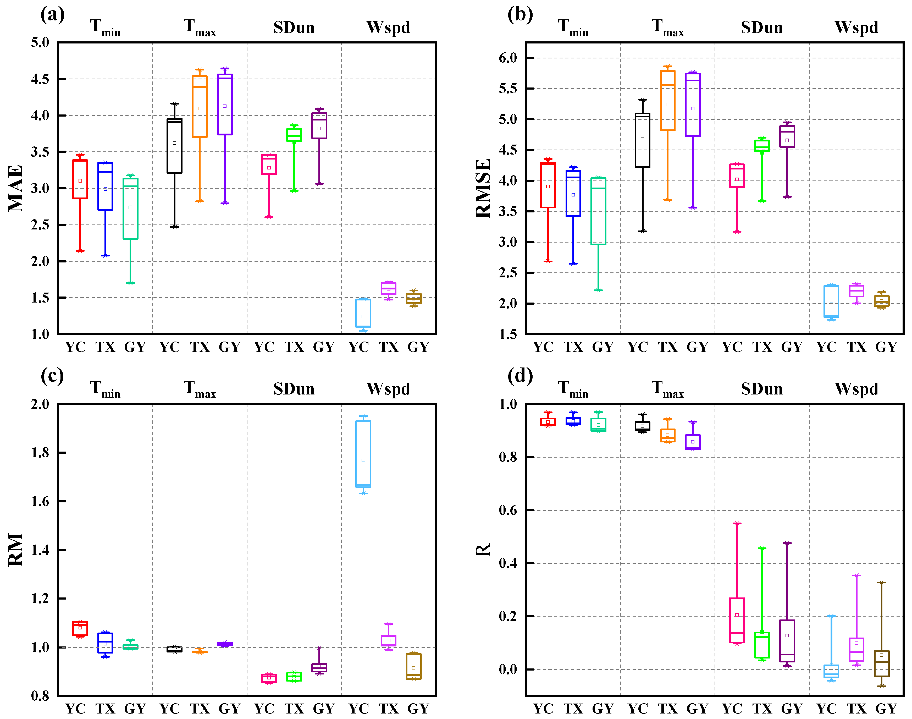
3.1.1. Single-Parameter Performance

The performance indicators of the daily scale forecast weather variables at the three study sites obtained from public weather forecasts with a lead time of 1–7 days for 2020–2021 are shown in Figure 3. The mean MAE and RMSE of T_min ranged from 2.73–3.10 °C and 3.51–3.90 °C, respectively. At the three sites, the mean MAE and RMSE of T_max ranged from 3.62–4.12 °C and 4.67–5.24 °C, respectively, while the mean R values of T_min and T_max were higher than 0.92 and 0.85, respectively. The accuracy of the T_min forecasts at all three sites was higher than that of the T_max forecasts, and the T_min and T_max prediction performance decreased with increasing forecast period, which is consistent with most previous studies in China [9,10,11,20,21,23,24,42,58,63]. In addition, the mean RM values of T_min and T_max ranged from 1.00–1.08 and 0.98–1.01, respectively, indicating that T_min was slightly overestimated at the three sites, T_max was slightly overestimated at GY, and T_max was slightly underestimated at YC and TX.

The mean MAE and RMSE of SDun at the three sites ranged from 3.28–3.82 h and 4.02–4.65 h, respectively, and the mean R and RM ranged from 0.13–0.20 and 0.88–0.92, respectively. The SDun forecast performance decreased in the order of YC, TX, and GY. SDun was underestimated by 12.51% (YC), 12.03% (TX), and 7.65% (GY). Compared to the temperature prediction performance, the SDun prediction performance was very poor, which may be due to the large error in the calculation process of converting the weather type in public weather forecast information into SDun [11,18,20,21,58].

The mean MAE and RMSE of Wspd at the three sites ranged from 1.24–1.61 m s⁻¹ and 1.98–2.19 m s⁻¹, respectively, and the mean R and RM ranged from 0.02–0.08 and 0.92–1.77, respectively. The Wspd prediction performance was poor at all stations. Wspd was overestimated by 76.78% (YC) and 2.79% (TX) and underestimated by 8.44% (GY). Among the four variables in public weather forecasts, Wspd exhibited the worst prediction performance, which may be caused by inadequate forecasts of the wind scale in public weather forecasts and errors in the conversion of the wind scale into the wind speed [18,20,21,42].

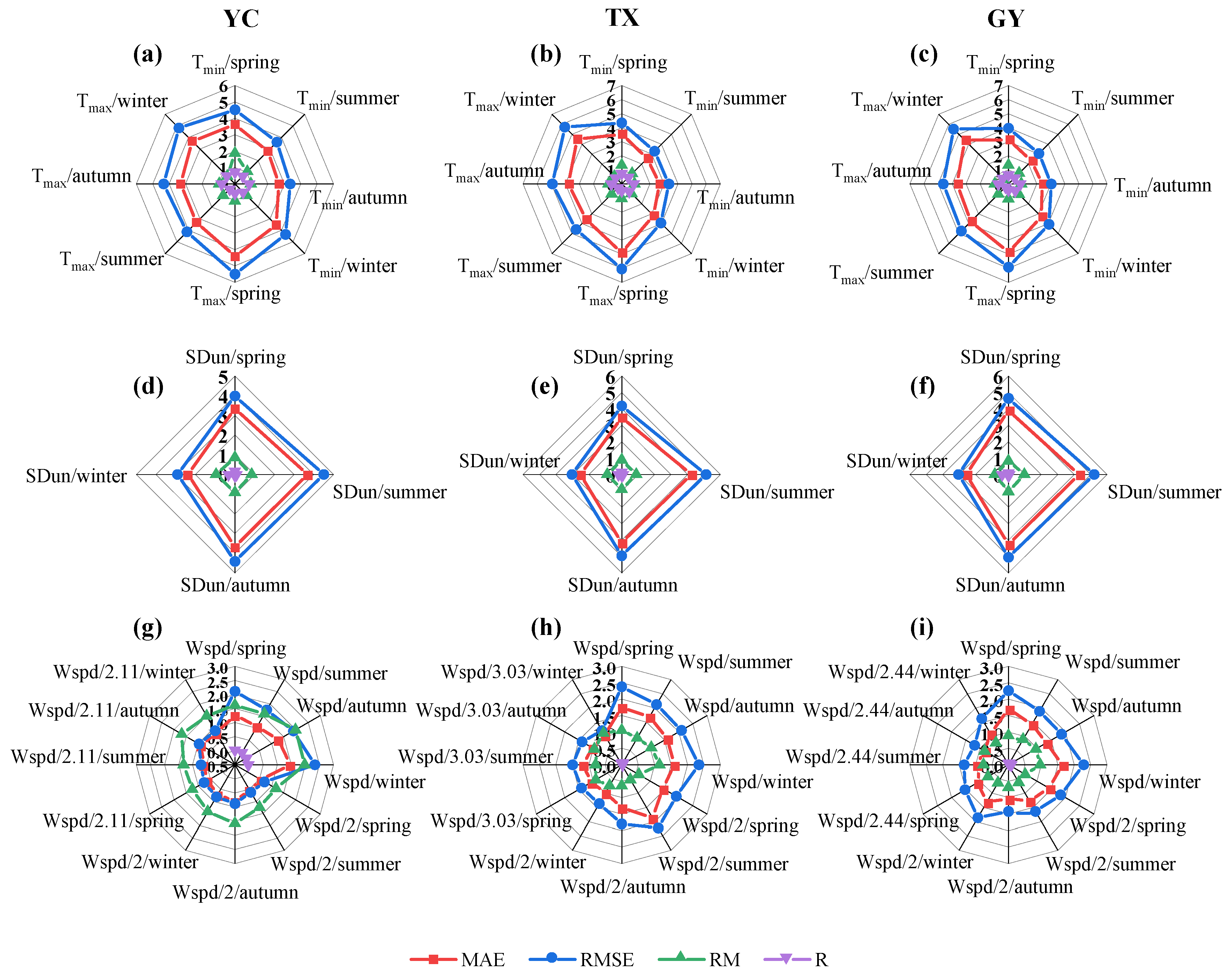
3.1.2. Seasonality of the Prediction Performance

The average seasonal statistics of the performance indicators of the weather variables predicted by public weather forecasts with a lead time of 1–7 days at the three research stations from 2020 to 2021 are shown in Figure 4. The average performance indicators of T_max at YC (GY) all decreased in the order of autumn, summer, winter, and spring. The average performance indicators of T_max at TX decreased in the order of summer, autumn, winter, and spring. At the three sites, T_max was overestimated within the range of 3.43–6.32% in spring (0.13–2.91% in summer) and underestimated within the range of 3.02–5.58% in autumn (26.21–57.24% in winter).

The average performance indicators of T_min at YC decreased in the order of autumn, summer, winter, and spring (autumn, summer, spring, and winter for GY). The average performance indicators of T_min in TX decreased in the order of summer, autumn, winter, and spring. At the three sites, T_min was overestimated within the range of 32.43–85.75% in spring (4.33–5.84% in summer) and underestimated within the range of 4.15–9.13% in autumn (0.49–1.28% in winter) (except T_min at GY, which was overestimated by 3.96% in winter).

The average performance indicators of SDun at the three sites decreased in the order of winter, spring, autumn, and summer. At the three sites, SDun was underestimated within the ranges of 11.89–18.08%, 3.52–15.18%, 8.96–8.99%, and 4.73–16.71% in spring, summer, autumn, and winter, respectively (except that SDun was overestimated by 3.76% in autumn at GY).

The predicted Wspd with a lead time of 1–7 days at the three research sites was defined as the predicted Wspd, a constant value (2 m s⁻¹) or the long-term daily average wind speed (2.11 m s⁻¹ at YC, 3.03 m s⁻¹ at TX, and 2.44 m s⁻¹ at GY). The average performance indicators of Wspd at YC during the four seasons decreased in the order of constant value, long-term daily average wind speed, and predicted Wspd. The average performance indicators when Wspd was defined as a constant value decreased in the order of summer, spring, winter, and autumn (summer, spring, autumn, and winter when the predicted Wspd was taken). Except in summer, the average performance indicators of Wspd at TX (GY) decreased in the order of long-term daily average wind speed, constant value, and predicted Wspd. Moreover, the average performance indicators at TX when Wspd was defined as a constant value decreased in the order of winter, autumn, spring, and summer (autumn, summer, winter, and spring when the predicted Wspd was taken). The average performance indicators at GY when Wspd was defined as a constant value and predicted Wspd decreased in the order of autumn, summer, winter, and spring. When Wspd was defined as a constant value (predicted Wspd), the predicted value at YC was overestimated by 17.92%, 24.84%, 59.04%, and 42.51% (62.03%, 59.62%, 98.80%, and 97.34%) in spring, summer, autumn, and winter, respectively, the predicted value at TX was underestimated by 39.96%, 47.71%, 36.30%, and 26.39% (overestimated by 5.13%, underestimated by 6.36%, overestimated by 4.14%, and overestimated by 14.78%) in spring, summer, autumn, and winter, respectively, and the predicted value at GY was underestimated by 40.96%, 37.80%, 31.30%, and 36.93% (11.06%, 10.99%, 3.98%, and 3.80%) in spring, summer, autumn, and winter, respectively.

In summary, according to the average seasonal statistics of the performance indicators of the weather variables predicted by the public weather forecasts with a lead time of 1–7 days at the three research sites from 2020 to 2021, the best T_max and T_min prediction performance occurred in autumn and summer, followed by winter and spring. The SDun prediction performance was consistent at the three sites, with the best performance in winter and spring, followed by autumn and summer, whereas the Wspd prediction performance greatly varied from site to site.

3.2. Calibration and Validation of the Three Empirical Equations

The calibration results of the three empirical equations of PMT, PMF, and HS at the three sites are provided in

Table 4. Best estimates of the corrected parameter for the three empirical equations at the three study sites.

Station	PMT			PMF		HS
	kRs	Tdew	WSpd	Tdew	WSpd	C	E
Yinchuan	0.16	Tdew = Tmin − 1	2 ms−1	Tdew = Tmin	2 ms−1	0.00096673	0.48475
Tongxin	0.21	Tdew = Tmin − 3	2 ms−1	Tdew = Tmin − 1	2 ms−1	0.00089671	0.53594
Guyuan	0.18	Tdew = Tmin − 2	2 ms−1	Tdew = Tmin	2 ms−1	0.00082219	0.55182

. The C and E values of the HS equation at the three sites occurred within the range given by Hu et al. [51].

The statistics of the ET_o prediction performance indicators of the three empirical equations (PMT, PMF, and HS) for the precalibration validation period and test period (a lead time of 1–7 days) and the postcalibration validation period and test period (a lead time of 1–7 days) are listed in

Table 5. Statistics based on the performance metrics of ET_o predicted with three empirical equations during the precalibration validation and test periods and the postcalibration validation and test periods.

Stage/Methods		Yinchuan				Tongxin				Guyuan
		MAE	RMSE	RM	R	MAE	RMSE	RM	R	MAE	RMSE	RM	R
		(mm d−1)	(mm d−1)			(mm d−1)	(mm d−1)			(mm d−1)	(mm d−1)
Uncalibrated
Training	PMT	0.40	0.60	0.92	0.96	0.44	0.66	0.93	0.96	0.37	0.54	0.94	0.96
	PMF	0.70	0.86	1.20	0.97	0.69	0.84	1.18	0.98	0.68	0.83	1.23	0.98
	HS	4.39	5.35	2.44	0.95	4.35	5.21	2.30	0.95	3.79	4.59	2.41	0.94
	PMT	0.39	0.56	0.91	0.96	0.51	0.73	0.90	0.96	0.35	0.50	0.93	0.96
	PMF	0.70	0.88	1.22	0.98	0.63	0.77	1.14	0.97	0.63	0.77	1.00	1.00
	HS	4.63	5.63	2.56	0.95	4.26	5.11	2.22	0.94	3.86	4.64	2.45	0.95
testing/the average of 1–7 days lead time
	PMT	0.63	0.89	1.03	0.88	0.99	1.36	0.90	0.80	0.92	1.22	0.92	0.72
	PMF	0.91	1.22	1.24	0.88	1.00	1.38	1.06	0.80	1.02	1.39	1.16	0.72
	HS	4.91	6.05	2.70	0.89	4.30	5.40	2.24	0.82	3.72	4.77	2.35	0.73
Calibrated
Validation	PMT	0.36	0.53	0.93	0.97	0.53	0.76	1.11	0.96	0.32	0.47	1.04	0.96
	PMF	0.80	1.00	1.25	0.97	0.58	0.72	1.11	0.96	0.64	0.79	1.22	0.98
	HS	0.46	0.62	1.04	0.95	0.54	0.76	0.95	0.94	0.38	0.51	0.99	0.95
testing/the average of 1–7 days lead time
	PMT	0.61	0.86	1.02	0.89	0.90	1.26	1.02	0.83	0.89	1.20	1.00	0.73
	PMF	0.86	1.17	1.21	0.88	0.95	1.31	1.03	0.81	0.99	1.36	1.14	0.72
	HS	0.68	0.97	1.09	0.89	0.95	1.31	0.96	0.81	0.94	1.26	0.95	0.72

. During the test period, the mean MAE, RMSE, and RM of the PMT equation at YC decreased from 0.63 mm d⁻¹, 0.89 mm d⁻¹, and 1.03 before calibration to 0.61 mm d⁻¹ and 0.86 mm d⁻¹ and 1.02 after calibration, respectively, and the mean R increased from 0.88 before calibration to 0.89 after calibration. Moreover, the average MAE, RMSE, and RM of the PMF equation at YC decreased from 0.91 mm d⁻¹, 1.22 mm d⁻¹, and 1.24 before calibration to 0.86 mm d⁻¹, 1.17 mm d⁻¹, and 1.21 after calibration, respectively. The average R changed only slightly before and after calibration, reaching a value of 0.88. The average MAE, RMSE, and RM of the HS equation at YC decreased from 4.91 mm d⁻¹, 6.05 mm d⁻¹, and 2.70 before calibration to 0.68 mm d⁻¹, 0.97 mm d⁻¹, and 1.09 after calibration, respectively. The average R remained almost unchanged before and after calibration, reaching a value of 0.89. After calibration, the performance of the three empirical equations in ET_o prediction was improved. Among them, the average MAE, RMSE, and RM of the HS equation for ET_o prediction decreased by 86.15%, 83.97%, and 59.63%, respectively. The three empirical equations attained a similar performance at TX and GY during the test period. The three empirical equations after calibration could be used to predict ET_o with a lead time of 1–7 days.

3.3. Performance Comparison of ET_o Prediction by the Four Machine Learning Algorithms under the Various Input Combinations

The performance statistics of the four machine learning models for daily ET_o prediction at YC, TX, and GY with a lead time of 1–7 days under the different input combinations are provided in Figure 5, Figure 6 and Figure 7, respectively, and the daily ET_o prediction performance significantly varied depending on the machine learning model, input combination of the machine learning model, and study site.

At YC, MLP and XGBoost performed best under the various input combinations during the training and validation periods. However, during the test period, the performance of the MLP, XGBoost, LightGBM, and CatBoost machine learning models in ET_o prediction under the different input combinations decreased in the order of C2, C4, C1, and C3. LightGBM was the best model for ET_o prediction under the C3 input combination (MAE = 0.83 mm d⁻¹, RMSE = 1.09 mm d⁻¹, and R = 0.85), while CatBoost attained the best prediction performance under all input combinations (MAE range: 0.69–0.77 mm d⁻¹; RMSE range: 0.93–0.99 mm d⁻¹; R range: 0.84–0.87). CatBoost achieved the highest performance with the C2 input combination (MAE = 0.69 mm d⁻¹, RMSE = 0.93 mm d⁻¹, and R = 0.86) during the testing phase at YC.

At TX, during the training and validation periods, MLP and XGBoost exhibited the best prediction performance under the C1 and C2 input combinations, while LightGBM and XGBoost achieved the best prediction performance under the C3 and C4 input combinations. However, during the test period, first, under the different input combinations, the ET_o prediction performance of MLP and LightGBM decreased in the order of C2, C1, C4, and C3, the ET_o prediction performance of XGBoost decreased in the order of C4, C2, C3, and C1, and the ET_o prediction performance of CatBoost decreased in the order of C3, C4, C2, and C1. Second, LightGBM attained the best prediction performance under the C1 and C2 input combinations (MAE range: 0.985–1.009 mm d⁻¹; RMSE range: 1.357–1.379 mm d⁻¹; R range: 0.78–0.79), while CatBoost achieved the best prediction performance under the C3 and C4 input combinations (MAE range: 0.95–0.96 mm d⁻¹; RMSE range: 1.279–1.31 mm d⁻¹; R range: 0.80–0.81). CatBoost was the best performing machine learning model for the C3 input combination (MAE = 0.95 mm d⁻¹, RMSE = 1.28 mm d⁻¹, R = 0.81) at TX during the test period.

At GY, during the training and validation periods, XGBoost and LightGBM exhibited the best prediction performance under the C1, C2, and C3 input combinations, while MLP and XGBoost exhibited the best prediction performance under the C4 input combination. However, during the test period, first, the ET_o prediction performance of the MLP under the different input combinations decreased in the order of C2, C1, C4, and C3, the ET_o prediction performance of XGBoost under the different input combinations decreased in the order of C2, C4, C1, and C3, and the ET_o prediction performance of LightGBM and CatBoost under the different input combinations decreased in the order of C4, C1, C2, and C3. Second, CatBoost was the best performing model for the C1, C2, and C4 input combinations (MAE range: 0.907–0.92 mm d⁻¹; RMSE range: 1.213–1.228 mm d⁻¹; R range: 0.699–0.707), and LightGBM was the best performing model for the C3 input combination (MAE = 0.95 mm d⁻¹; RMSE = 1.28 mm d⁻¹; R = 0.68). CatBoost was the best performing machine learning model for the C4 input combination (MAE = 0.907 mm d⁻¹; RMSE = 1.213 mm d⁻¹; R = 0.707) at GY during the test period.

The best input combinations of the four machine learning models, i.e., MLP, XGBoost, LightGBM, and CatBoost, and their model tuning information are provided in

Table 6. Optimal input combinations and model tuning information of the four machine learning methods at the three meteorological stations.

Station	MLP			XGBoost	LightGBM	CatBoost
	Inputs	Structure	Parameter Value	Inputs	Inputs	Inputs
Yinchuan	C2	3-100-100-100-1	Lr = 0.0088	C2	C2	C2
Tongxin	C2	3-85-85-1	Lr = 0.0088	C4	C2	C3
Guyuan	C2	3-62-62-1	Lr = 0.0055	C2	C4	C4

. The best input combination of CatBoost at TX was C3 (8.33%). In contrast, the best input combination of the four machine learning models at the three sites was C2 (66.67%) or C4 (25.00%), indicating that the addition of SDun to the input combination positively affected the improvement in the ET_o prediction performance of the four machine learning models [1,11,20,31,58,63,67,68]. Since the predicted Wspd exhibits the worst prediction performance among the variables in the public weather forecasts, the addition of the predicted Wspd to the input combination could lead to a decrease in the daily ET_o prediction performance of the machine learning models (except for the CatBoost model at TX), which is consistent with previous research results [42]. In addition, the MLP with two–three hidden layers performs better in predicting daily ET_o than the MLP with only one hidden layer [10,56,58].

3.4. ET_o Prediction Performance Evaluation of the Seven Models Based on Public Weather Forecasts

3.4.1. Daily ET_o Prediction Performance of the Seven Models

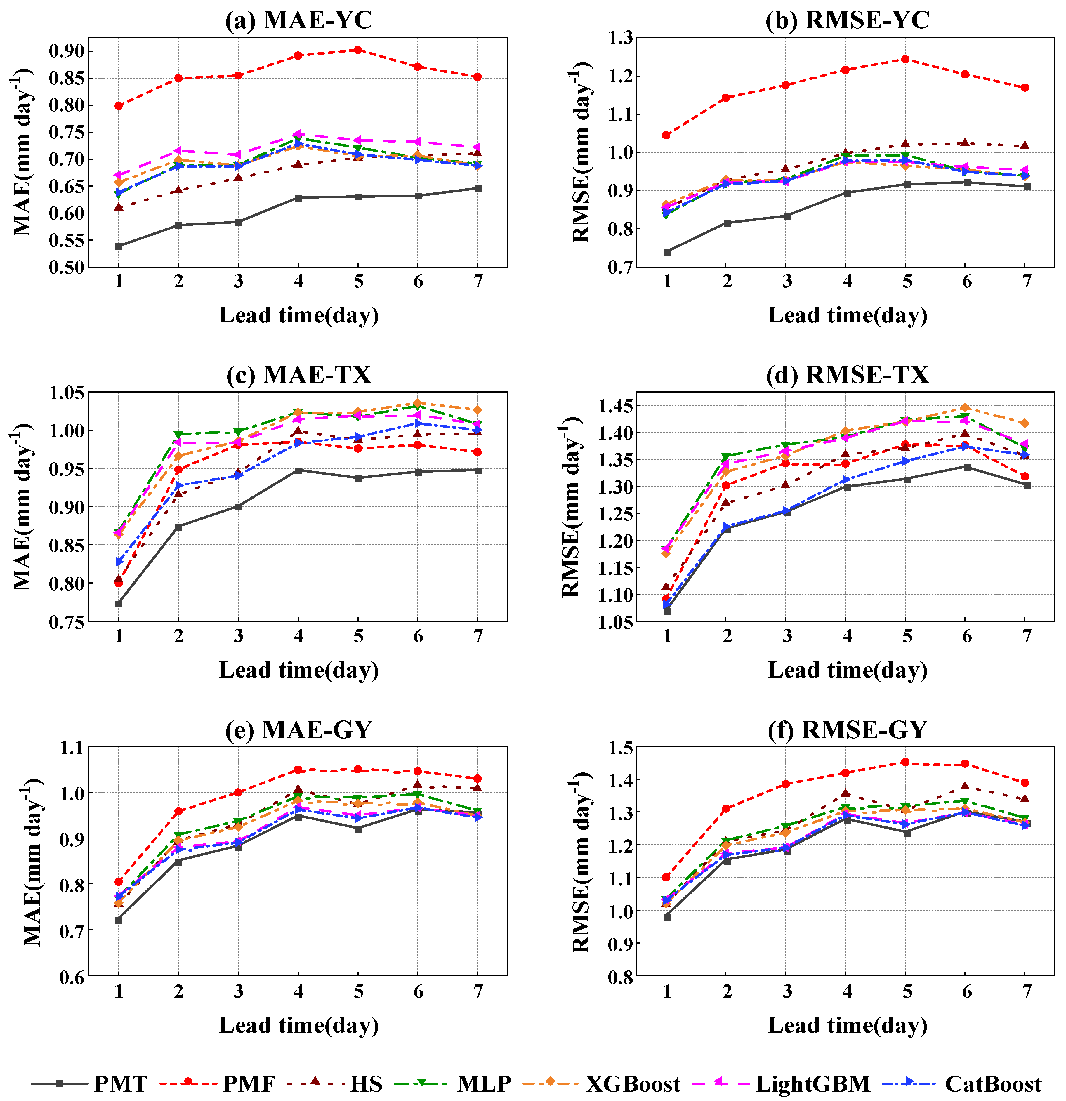
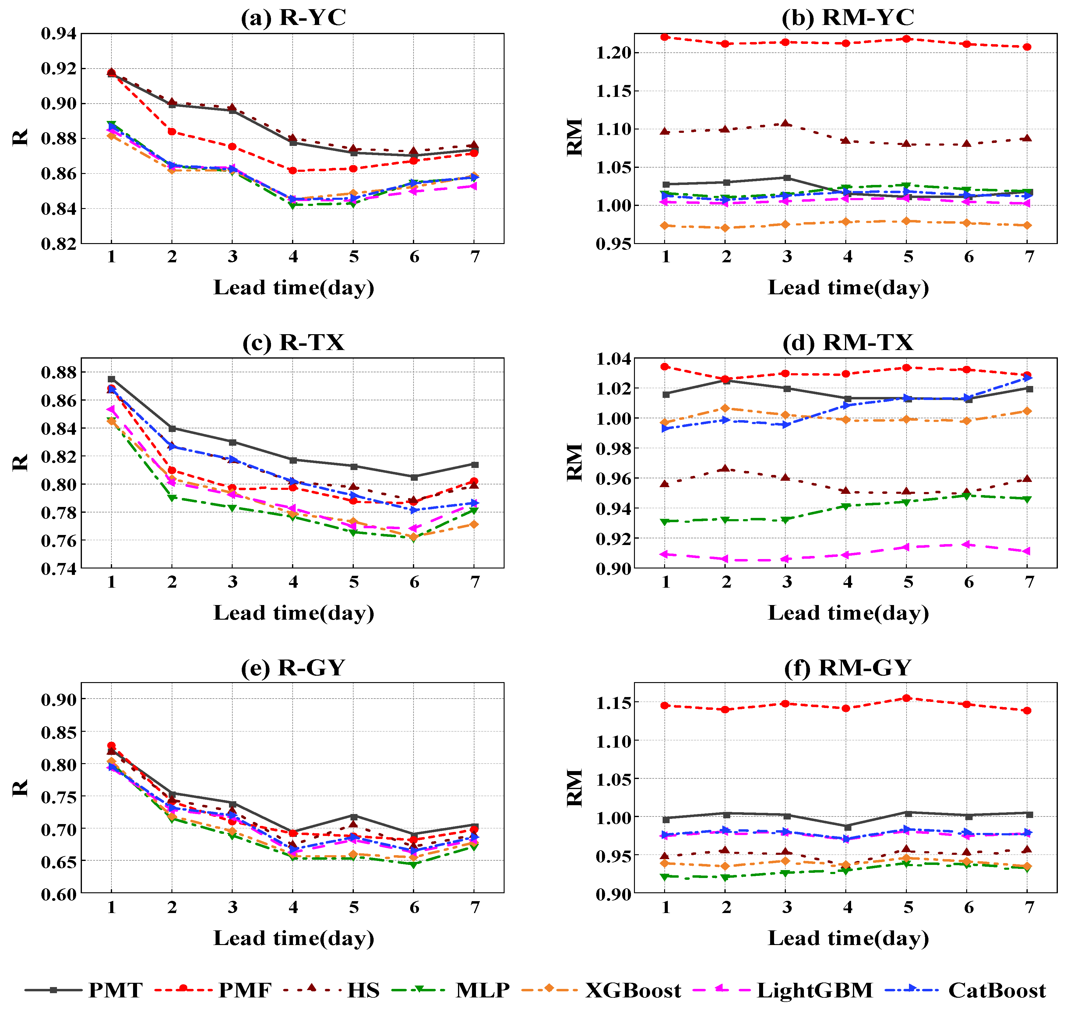
The daily ET_o prediction performance indicators of the three empirical equations and four machine learning models with a lead time of 1–7 days at the three sites are shown in Figure 8 and Figure 9, respectively. First, the daily ET_o prediction performance of the seven models at YC, TX, and GY decreased with increasing lead time, which is due to the decrease in the performance of the public weather forecast variables with increasing lead time, which is consistent with previous research results [1,2,9,10,11,17,20,23,42,58,63]. Second, the RM values of the 7 models at YC ranged from 0.97 to 1.22, among which the XGBoost model slightly underestimated (2.04–2.96%) the daily ET_o, the PMF equation overestimated (20.74–22.03%) the daily ET_o, and the other models slightly overestimated (0.24–10.68%) the daily ET_o. The RM values of the seven models at TX ranged from 0.91 to 1.03, among which the HS, MLP, and LightGBM models slightly underestimated (3.39–9.38%) the daily ET_o, while the other models slightly overestimated (0.46–3.43%) the daily ET_o. The RM values of the seven models at GY ranged from 0.92 to 1.15. The PMF equation overestimated (13.83–15.46%) the daily ET_o, and the PMT equation slightly overestimated (0.19–0.47%) the daily ET_o, while the other models slightly underestimated (1.67–7.93%) the daily ET_o. The PMF model overestimated the daily ET_o at YC, which may be due to Wspd overestimation at this site. Under arid conditions, the drier the atmosphere is, the more small changes in wind speed could lead to large changes in the evapotranspiration rate and thus the greater the impact on evapotranspiration [36]. The daily ET_o overestimation by the PMF model noted at GY may be due to T_max overestimation at this site. Moreover, the overestimation percentage of T_max at GY was higher than that of T_min, and the saturation vapor pressure was overestimated due to T_max overestimation, resulting in an increase in the saturation vapor pressure deficit and overestimation of the daily ET_o at GY.

Table 7. Mean statistics of the performance indicators for ET_o prediction with a lead time of 1–7 days by the seven methods at the three sites.

Method	Yinchuan				Tongxin				Guyuan
	MAE	RMSE	RM	R	MAE	RMSE	RM	R	MAE	RMSE	RM	R
	(mm d−1)	(mm d−1)			(mm d−1)	(mm d−1)			(mm d−1)	(mm d−1)
PMT	0.61	0.862	1.02	0.89	0.90	1.257	1.02	0.83	0.89	1.20	1.00	0.73
PMF	0.86	1.17	1.21	0.88	0.949	1.307	1.03	0.807	0.99	1.36	1.15	0.72
HS	0.675	0.971	1.09	0.89	0.949	1.309	0.96	0.814	0.94	1.26	0.95	0.72
MLP	0.70	0.938	1.02	0.86	0.991	1.362	0.94	0.786	0.94	1.25	0.93	0.69
XGBoost	0.70	0.936	0.98	0.86	0.989	1.363	1.00	0.789	0.923	1.234	0.94	0.70
LightGBM	0.72	0.938	1.01	0.86	0.985	1.358	0.91	0.793	0.911	1.217	0.98	0.70
CatBoost	0.691	0.933	1.01	0.86	0.954	1.279	1.01	0.811	0.908	1.214	0.98	0.71

Note: The statistical indicators of the best performing model at each site are shown in bold and the statistical indicators of the favorable models are highlighted in gray.

shows the mean statistics of the performance metrics for the predicted daily ET_o with a lead time of 1–7 days by the seven models at the three sites. Combining all indicators, first, the prediction performance of the seven models at YC was better than that at TX and GY, which is mainly due to the overall better forecast performance of the public weather forecast variables at YC than at TX and GY. Second, the top three models at YC were PMT, HS, and CatBoost, whereas PMF (the worst performing model) overestimated the daily ET_o (21.35%). The top three models at TX were PMT, CatBoost, and HS, whereas MLP (the worst performing model) underestimated the daily ET_o (6.05%), and the top three models at GY were PMT, CatBoost, and LightGBM, whereas PMF (the worst model) overestimated the daily ET_o (14.46%).

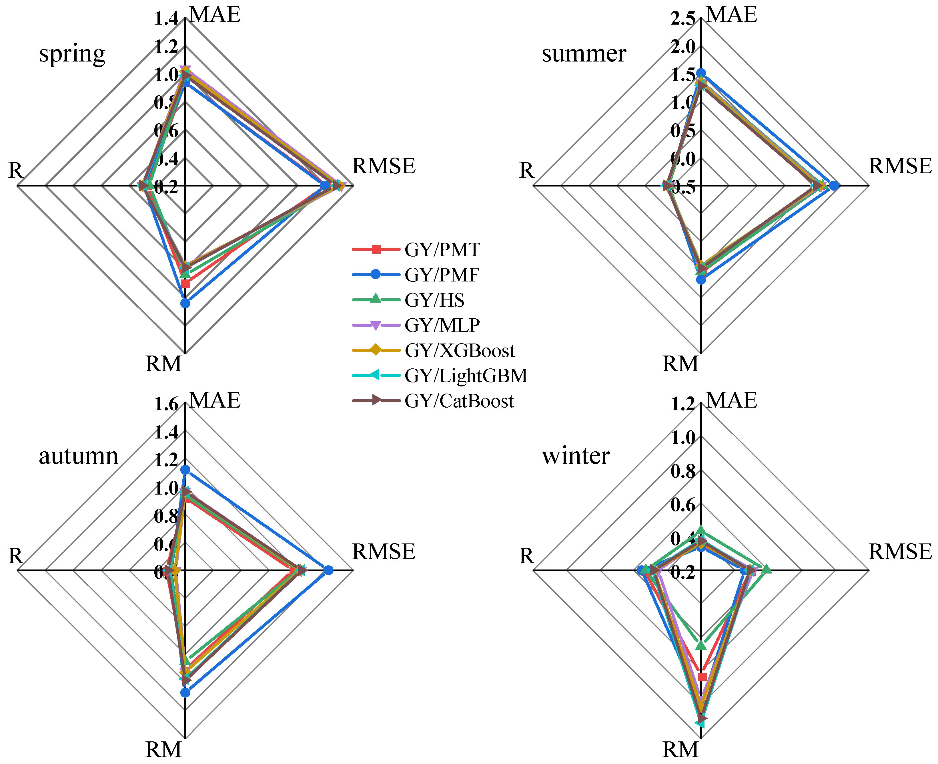
3.4.2. Seasonality of the Daily ET_o Prediction Performance of the Seven Models

The sensitivity of weather variables varies with the different seasons and the microclimate at the studied site location [15], while the irrigation area at the studied site location is associated with different field irrigation periods depending on the crop type, location, etc. [1]. Therefore, it is necessary to evaluate the seasonality of the ET_o prediction performance. The average ET_o prediction performance indicators with a lead time of 1–7 days of the seven methods at the three station sites during the four seasons from 2020–2021 are shown in Figure 10, Figure 11 and Figure 12, respectively.

First, during all four seasons, the daily ET_o prediction performance of all seven models was higher at YC than at TX and GY (excluding the LightGBM model in winter), which was consistent with the results of evaluating the performance of daily ETo predicted by the seven models at three research sites (YC, TX, and GY) from a daily scale.

Second, except for the LightGBM model at TX, the seasonal MAE and RMSE values for ET_o prediction of all seven models at YC and six models at TX increased in the order of winter, spring, autumn, and summer, and the seasonal MAE and RMSE values in winter and spring were smaller than the annual values. At GY, except for the PMF model, the seasonal MAE and RMSE values for ET_o prediction of the other six models increased in the order of winter, autumn, spring, summer, and the seasonal MAE and RMSE values in winter were smaller than the annual values. This is consistent with previous studies [1,16,20]. The seasonal R values for ET_o prediction of all models at the three sites were smaller than the annual values, and the seasonal R values were the smallest in summer. The seasonal R values at YC were the largest in autumn (except for the PMF model), the seasonal R values at TX were the largest in spring (the three empirical equations and the CatBoost model) and winter (MLP, XGBoost, and LightGBM), and the seasonal R values at GY were the largest in spring (MLP, XGBoost, and LightGBM), autumn (LightGBM and CatBoost), and winter (the three empirical equations). The seasonal RM values for daily ET_o prediction by the four machine learning models at the three sites were less than one in spring and summer and greater than one in autumn and winter, indicating that the daily ET_o in spring and summer was underestimated, while the daily ET_o was overestimated in autumn and winter (except at GY, where the MLP model underestimated the daily ET_o by 3.20%). The seasonal RM values for daily ET_o prediction by the three empirical models at YC and GY in summer and autumn and at TX in autumn were all greater than 1, indicating that the daily ET_o was overestimated during the corresponding season.

Finally, combining all indicators, at YC, the indicators of the predicted seasonal ET_o values with a lead time of 1–7 days by PMT were the best during all seasons, followed by HS (spring, autumn, and winter) and CatBoost (summer). At TX, the indicators of the predicted seasonal ET_o values with a lead time of 1–7 days by PMT were the best in spring, autumn, and winter. The indicators of the predicted seasonal ET_o values with a lead time of 1–7 days by CatBoost were the best in summer, followed by PMF (spring), PMT (summer), and LightGBM (autumn and winter). 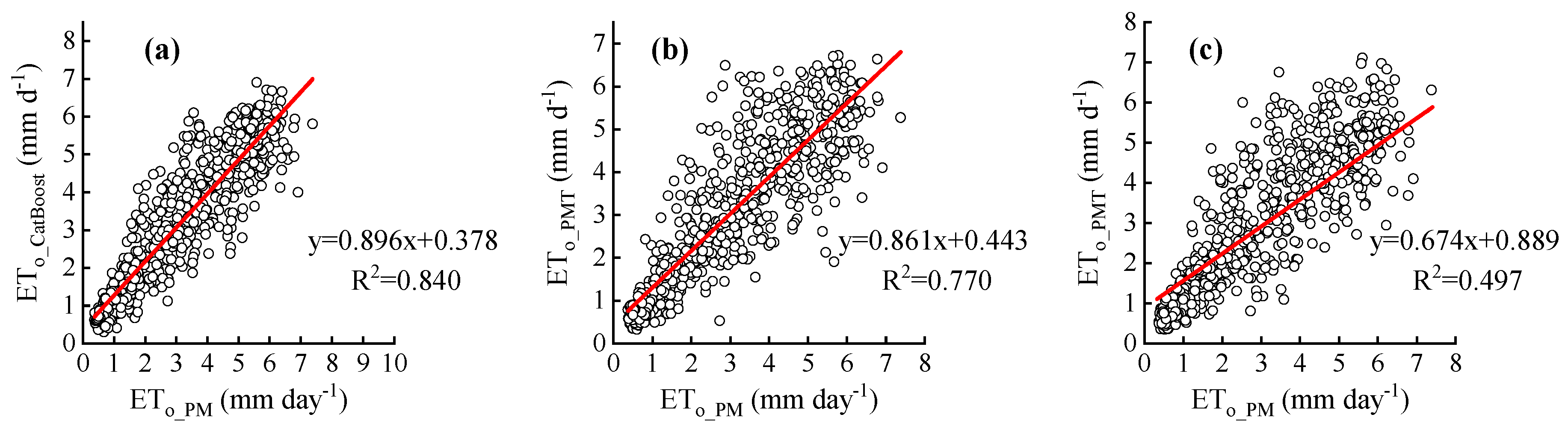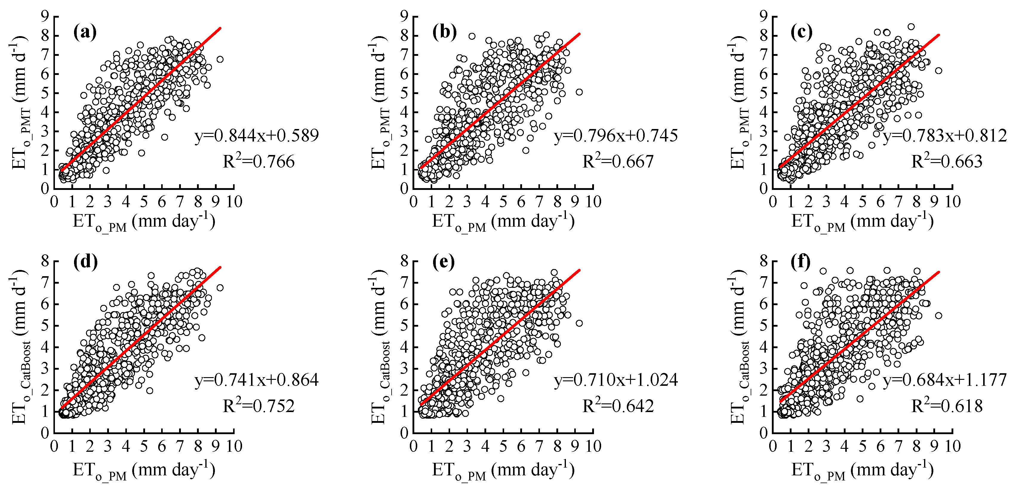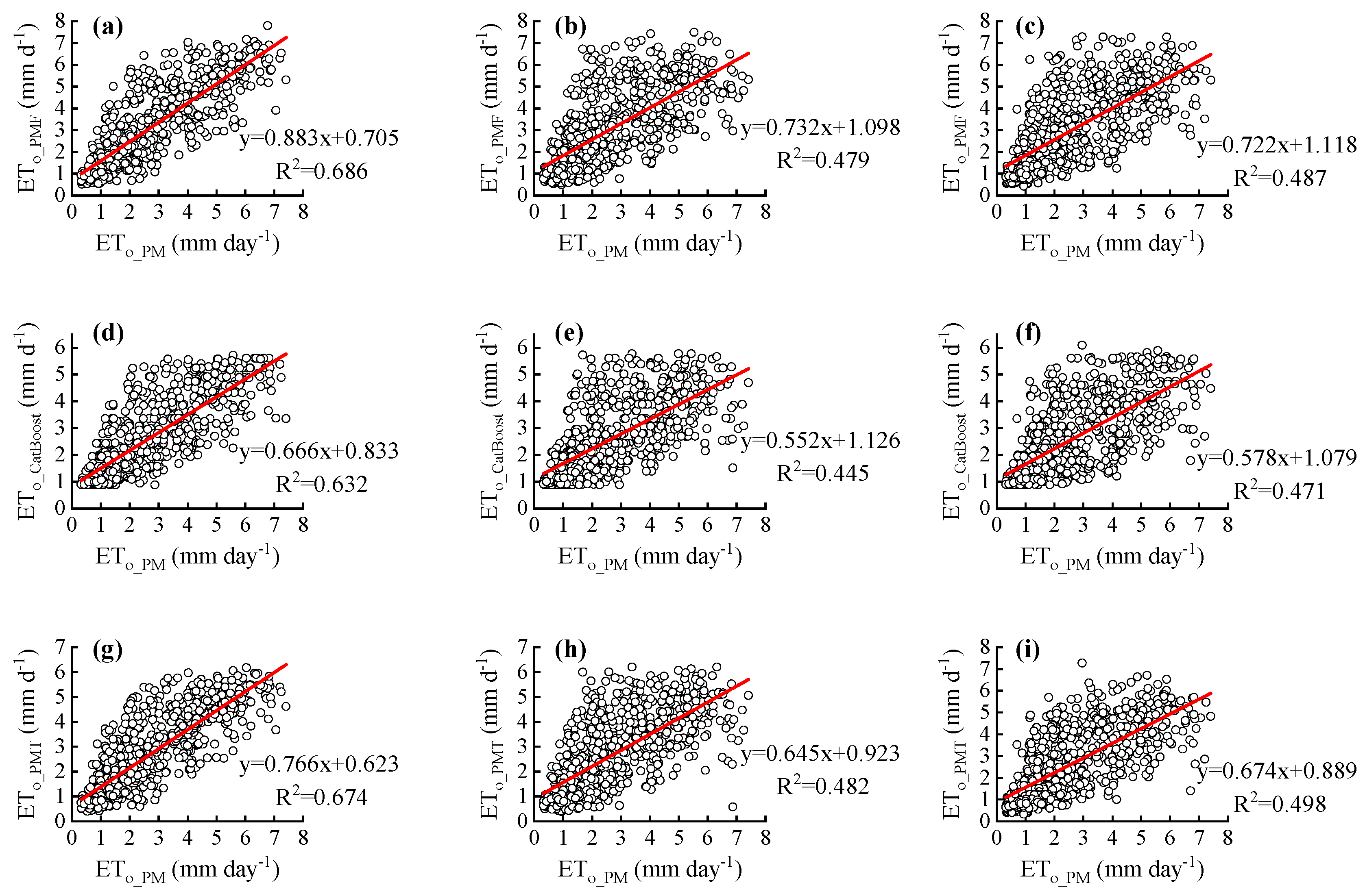At GY, the indicators of the predicted seasonal ET_o values with a lead time of 1–7 days by PMF were the best in spring and winter, those of the predicted seasonal ET_o values with a lead time of 1–7 days by CatBoost were the best in summer, and those of the predicted seasonal ET_o values with a lead time of 1–7 days by PMT were the best in autumn, followed by PMT (spring and winter), LightGBM (summer), and HS (autumn). The scatter plots of the daily ET_o predicted by the PMT equations for the test period versus the daily ET_o computed by the PM equations for YC station; the scatter plots of the daily ET_o predicted by the PMT equations and the CatBoost model for the test period versus the daily ET_o computed by the PM equations for TX station; and the scatter plots of the daily ET_o predicted by the PMF equations, the CatBoost model, and the PMT equations for the test period versus the daily ET_o computed by the PM equations for GY station are given in Figure 13, Figure 14 and Figure 15, respectively.

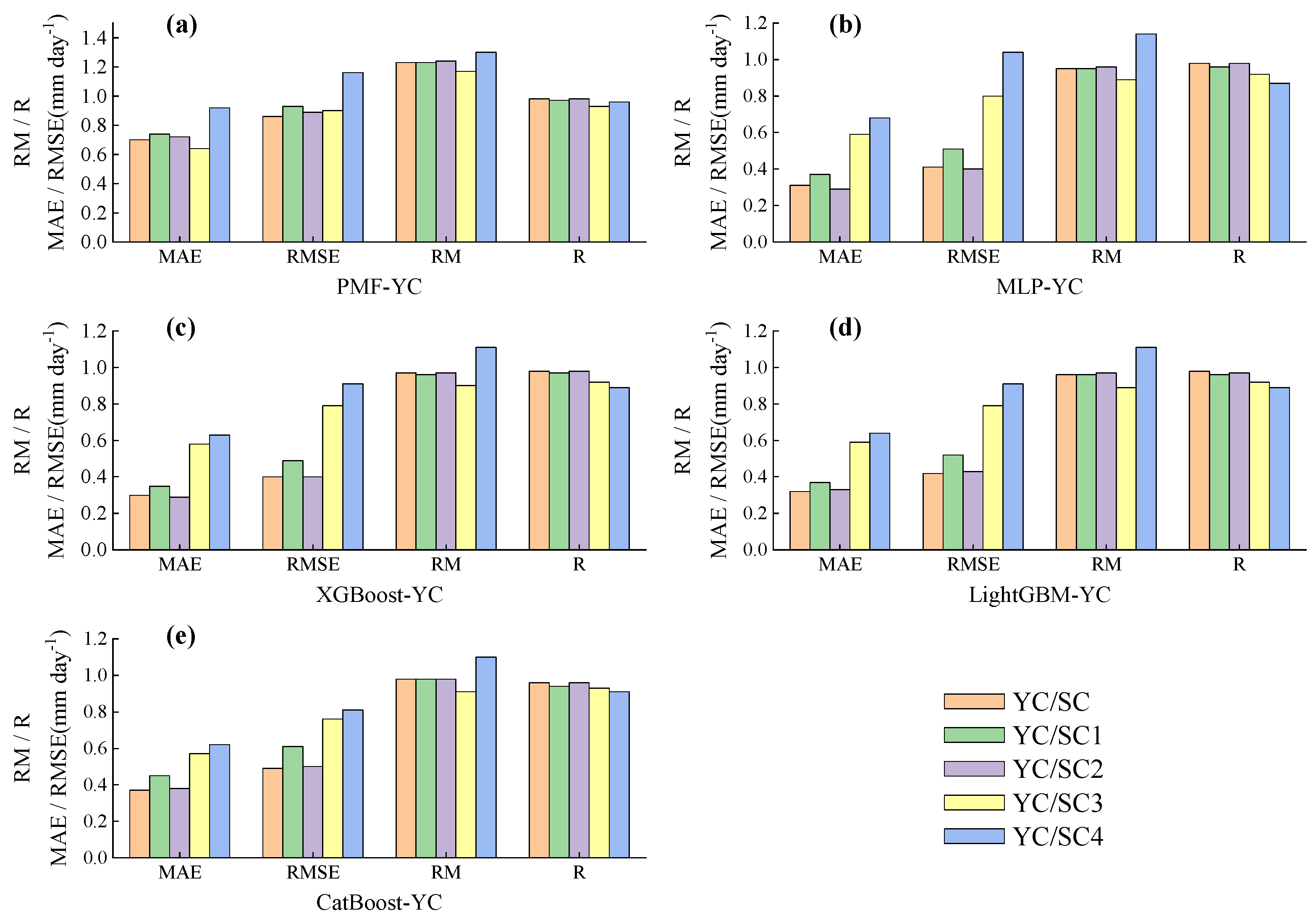
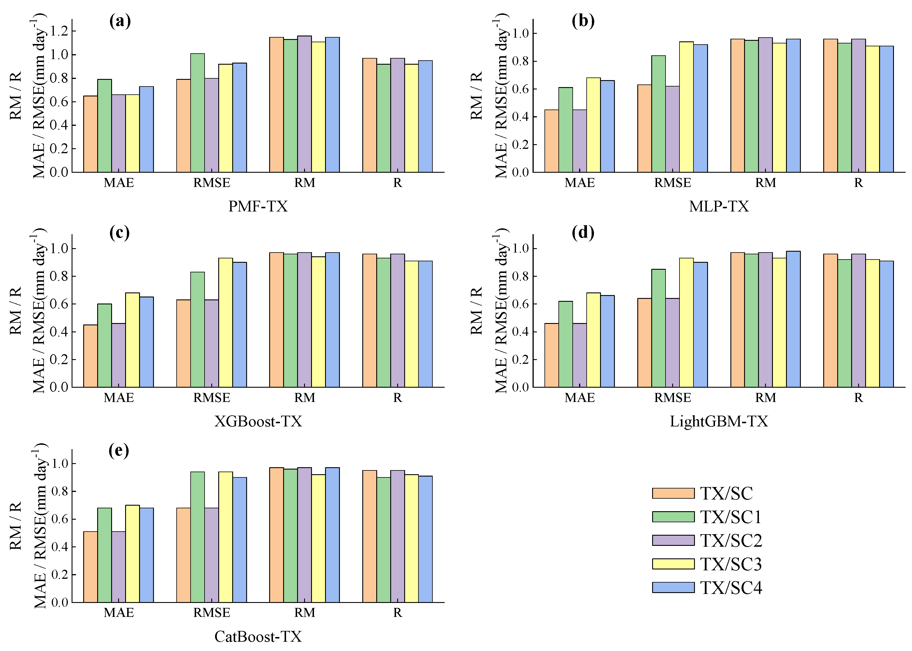
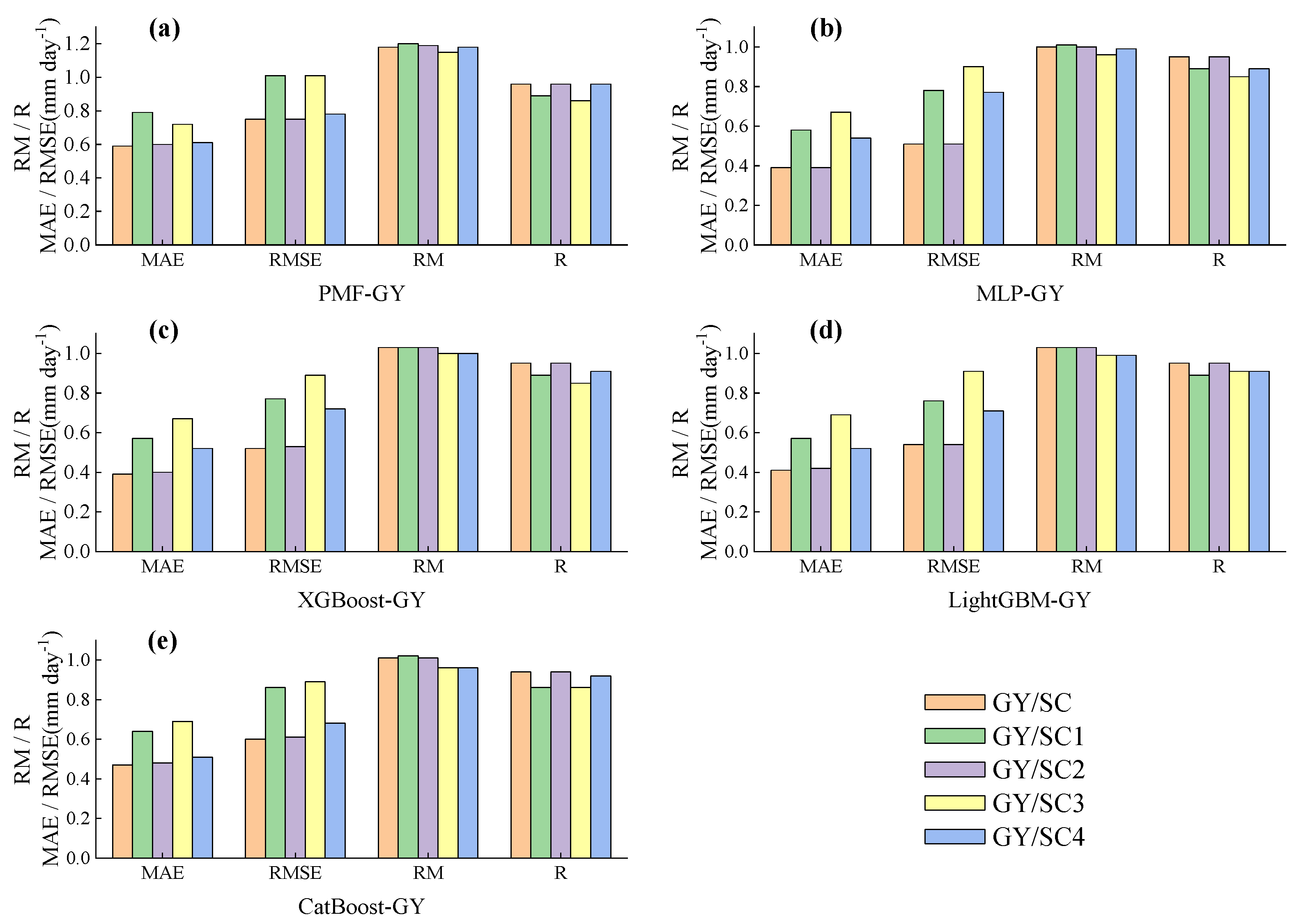
3.5. Impact of Weather Variable Prediction Based on Public Weather Forecasts on Daily ET_o Prediction

To assess the impact of the weather variables in public weather forecasts on the performance of daily ET_o prediction, the four observed weather variables (T_max, T_min, SDun, and Wspd) were replaced in sequence with corresponding forecast values for a lead time of 1–7 days, such that a large change in the forecasted daily ET_o indicates that the forecasted weather variable would produce a large error in daily ET_o prediction [1,13,16,20]. T_max, T_min, Sdun, and Wspd in public weather forecasts with a lead time of 1–7 days were used to replace the corresponding daily observed values of T_max, T_min, SDun, and Wspd, respectively, to form new combinations, namely, SC1 (T_max, T_min, SDun, and Wspd), SC2 (T_max, T_min, SDun, and Wspd), SC3 (T_max, T_min, SDun, and Wspd), and SC4 (T_max, T_min, SDun, and Wspd). The combination of all observations was denoted as SC (T_max, T_min, SDun, and Wspd). The mean values of the ET_o performance indicators of the five models at the three sites under the SC-SC4 input combinations are provided in Figure 16, Figure 17 and Figure 18.

First, for the five models at all stations, the daily ET_o slightly differed before and after replacing the observed T_min with T_min of the public weather forecasts. Notably, T_min exhibited the smallest prediction error, and its contribution to the error in daily ET_o prediction was minimal.

Second, for all models at YC, Wspd yielded the largest contribution to the error in the predicted daily ET_o (first), and for the four machine learning models, SDun and T_max yielded large (second) and relatively small (third) contributions, respectively, to the error in the predicted daily ET_o, which is consistent with previous findings [20]. Regarding the PMF model, T_max and SDun also yielded large (second) and relatively small (third) contributions, respectively, to the error in the predicted daily ET_o. At TX, among the four machine learning models, n contributed the most to the error in the predicted daily ET_o (first), and Wspd and T_max greatly contributed to the error in the predicted daily ET_o (second or third). Moreover, T_max contributed the most to the error in the predicted daily ET_o by the PMF model (first), while Wspd and SDun greatly contributed to the error in the predicted daily ET_o (second and third, respectively). For all models at GY, SDun contributed the most to the error in the predicted daily ET_o (first), while T_max and Wspd also greatly contributed (second and third, respectively) to the error in the predicted daily ET_o. This is consistent with previous studies [12,13,16,20].

These results indicate that the main source of error in daily ET_o prediction at YC in an arid region is Wspd transformed from the wind scale in public weather forecasts. Due to regional differences, as well as the influences of the location of weather stations and local topographic features [42], wind speed is one of the most difficult parameters to accurately predict [20,69]. Cai et al. [18] stated that it is acceptable to estimate the wind speed from the wind scale in public weather forecasts, but the error in such estimates could be large in arid regions [20]. George et al. [70] showed that the discrepancy between predicted and measured reference crop evapotranspiration values largely resulted from erroneous predictions of the mean wind speed. Li and Beswick [71] reported that wind speed represents a more serious source of error than solar radiation in ET_o estimation. Except in arid and windy areas, the effect of the wind speed on the estimated ET_o values is relatively limited [72].

At TX in a semiarid region and GY in a semihumid region, SDun converted from the weather type in public weather forecasts was the main source of error in daily ET_o prediction. First, since the weather type in the public weather forecasts was converted into SDun using the sunshine duration coefficient values listed in Table 3, obtained using 2004 measured solar radiation data for Daxing District, Beijing, which is located in a warm temperate semihumid continental monsoon climate zone, the application of sunshine duration coefficients derived from one region to other regions with different climate types could result in different degrees of error due to the climatic differences between these regions [11,21]. Second, the values of a_s and b_s in Equation (11) can vary depending on atmospheric conditions (humidity and dust) and solar declination (latitude and month), so the improved a_s and b_s parameters must be calibrated when calculating R_s with Equation (11) [36]; in contrast, we directly used the recommended values of 0.25 and 0.5 without calibration, which could also cause errors. Perera et al. [1] found that the largest error source between predicted and observed ET_o values is the prediction accuracy of the incident solar radiation. The results of Medina et al. [13] showed that the error in radiation prediction imposed the greatest influence on ET_o prediction, followed by the error in wind prediction. Fan et al. [16] noted that in the temperate continental zone (TCZ), temperate monsoon zone (TMZ), and other climate zones, the contribution of the R_s (solar radiation) prediction error to the ET_o prediction error was the greatest.

4. Conclusions

In this study, the performance of three empirical equations and four machine learning models for daily ET_o prediction at three stations in three climatic regions of Ningxia, China, was evaluated using public weather forecasts with a lead time of 1–7 days. The prediction performance of weather variables in public weather forecasts and the prediction performance of the daily ET_o of the seven models were analyzed and evaluated on daily and seasonal scales, respectively. The optimal input combination of the machine learning models was determined, and the weather forecast variables contributing to the error in the predicted daily ET_o were clarified. The main conclusions of this study are as follows:

(1)

At all stations, in the public weather forecast variables with a lead time of 1–7 days during the four seasons of spring, summer, autumn and winter from 2020–2021, T_max followed the order of autumn > summer> winter > spring (or summer > autumn > winter > spring), T_min followed the order of autumn > summer > winter > spring (or summer > autumn) > spring > winter), SDun followed the order of winter > spring > autumn > summer, and the average forecast performance decreased in sequence. The performance of wind speeds predicted by public weather forecasts was the worst, and their prediction performance showed great variation depending on the station. It was recommended that the model predict the daily ET_o by considering the wind speed to take a constant value (2 m s⁻¹) or the daily average wind speed over a long period;

(2)

The calibrated PMT equation (k_Rs = 0.16, T_dew = T_min − 1) with public weather forecasts of T_max, T_min, and 2 m s⁻¹ of constant wind speed as inputs was recommended as the best model for the irrigation season at YC station for the predicted lead time of 1–7 day ET_o for all three stations. The calibrated PMT equation (k_Rs = 0.21, T_dew = T_min − 3) with public weather forecasts of T_max, T_min, and constant wind speed of 2 m s⁻¹ as inputs and CatBoost with C3 (T_max, T_min, Wspd) as inputs were the best-performing models for the spring and autumn irrigation seasons and the summer irrigation season at station TX, respectively. The calibrated PMF equation (T_dew = T_min) with T_max, T_min, SDun, and 2 m s⁻¹ constant wind speed from the public weather forecast as inputs, CatBoost with C4 (T_max, T_min) as inputs, and the calibrated PMT equation (kr = 0.18, T_dew = T_min−2) with T_max, T_min, and 2 m s⁻¹ constant wind speed from the public weather forecast as inputs were the optimal models for the spring irrigation season, summer irrigation season, and autumn irrigation season, respectively, at the GY station;

(3)

The four machine learning models MLP, XGBoost, LightGBM, and CatBoost are recommended to select C2 (T_max, T_min, SDun) or C4 (T_max, T_min) as the input combinations to predict the daily ET_o of the three stations. However, for station YC located in the arid zone, the error in the model prediction of daily ET_o is mainly caused by Wspd from the public weather forecast, followed by SDun. SDun from the public weather forecast is the main source of error in the model prediction of daily ET_o for station TX located in the semiarid zone and station GY located in the semimoisture zone, followed by Wspd. Therefore, the combination of Wspd from public weather forecasts and SDun should be considered carefully when adding them to the input combination of the model.

The optimal predictive daily ET_o model for the irrigation season recommended in this study has been successfully used in the irrigation forecast of 1–3 days in advance for 134 ha of Lycium barbarum crop in Tongxin, Ningxia, China. Compared with the local conventional irrigation, the irrigation forecasting of 1–3 days in advance using the ET_o model of the optimal prediction day of the irrigation season realized the improvement of quality and yield, and water-saving irrigation of field Lycium barbarum, and improved the utilization of the limited rainfall during the fertility period of the Lycium barbarum crop.

Although the best models for predicting daily ET_o during the irrigation season at the study stations were obtained, some stations had lower model prediction accuracy during certain irrigation seasons (e.g., the best models for the summer season at the TX and GY stations), and the combination of these machine learning models with optimization algorithms (ant colony optimization algorithms, cuckoo search algorithms, flower pollination algorithms, etc.) could be explored to optimize the model’s hyperparameters through optimization algorithms to further enhance the performance of the model to predict ET_o and improve the accuracy of the model to predict ET_o.

References

1. Perera, K.C.; Andrew, W.W.; Bandara, N.; Biju, G. Forecasting daily reference evapotranspiration for Australia using numerical weather prediction outputs. Agric. For. Meteorol. 2014, 194, 50–63. [Google Scholar] [CrossRef]
2. Traore, S.; Luo, Y.; Fipps, G. Gene-expression programming for short-term forecasting of daily reference evapotranspiration using public weather forecast information. Water Resour. Manag. 2017, 31, 4891–4908. [Google Scholar] [CrossRef]
3. Aghelpour, P.; Norooz-Valashedi, R. Predicting daily reference evapotranspiration rates in a humid region, comparison of seven various data-based predictor models. Stoch. Environ. Res. Risk Assess. 2022, 36, 4133–4155. [Google Scholar] [CrossRef]
4. Torres, A.F.; Walker, W.R.; McKee, M. Forecasting daily potential evapotranspiration using machine learning and limited climatic data. Agric. Water Manag. 2011, 98, 553–562. [Google Scholar] [CrossRef]
5. Kim, S.; Shiri, J.; Singh, V.P.; Kisi, O.; Landeras, G. Predicting daily pan evaporation by soft computing models with limited climatic data. Hydrol. Sci. J. 2015, 60, 1120–1136. [Google Scholar] [CrossRef]
6. Ferreira, L.B.; da Cunha, F.F. Multi-step ahead forecasting of daily reference evapotranspiration using deep learning. Comput. Electron. Agric. 2020, 178, 105728. [Google Scholar] [CrossRef]
7. Ruiming, F.; Shijie, S. Daily reference evapotranspiration prediction of Tieguanyin tea plants based on mathematical morphology clustering and improved generalized regression neural network. Agric. Water Manag. 2020, 236, 106177. [Google Scholar] [CrossRef]
8. Karbasi, M.; Jamei, M.; Ali, M.; Malik, A.; Yaseen, Z.M. Forecasting weekly reference evapotranspiration using Auto Encoder Decoder Bidirectional LSTM model hybridized with a Boruta-CatBoost input optimizer. Comput. Electron. Agric. 2022, 198, 107121. [Google Scholar] [CrossRef]
9. Luo, Y.; Chang, X.; Peng, S.; Khan, S.; Wang, W.; Zheng, Q.; Cai, X. Short-term forecasting of daily reference evapotranspiration using the Hargreaves–Samani model and temperature forecasts. Agric. Water Manag. 2014, 136, 42–51. [Google Scholar] [CrossRef]
10. Luo, Y.; Traore, S.; Lyu, X.; Wang, W.; Wang, Y.; Xie, Y.; Jiao, X.; Fipps, G. Medium range daily reference evapotranspiration forecasting by using ANN and public weather forecasts. Water Resour. Manag. 2015, 29, 3863–3876. [Google Scholar] [CrossRef]
11. Yang, Y.; Luo, Y.; Wu, C.; Zheng, H.; Zhang, L.; Cui, Y.; Sun, N.; Wang, L. Evaluation of six equations for daily reference evapotranspiration estimating using public weather forecast message for different climate regions across China. Agric. Water Manag. 2019, 222, 386–399. [Google Scholar] [CrossRef]
12. Pelosi, A.; Medina, H.; Villani, P.; D’urso, G.; Chirico, G. Probabilistic forecasting of reference evapotranspiration with a limited area ensemble prediction system. Agric. Water Manag. 2016, 178, 106–118. [Google Scholar] [CrossRef]
13. Medina, H.; Tian, D.; Srivastava, P.; Pelosi, A.; Chirico, G.B. Medium-range reference evapotranspiration forecasts for the contiguous United States based on multi-model numerical weather predictions. J. Hydrol. 2018, 562, 502–517. [Google Scholar] [CrossRef]
14. Medina, H.; Tian, D. Comparison of probabilistic postprocessing approaches for improving numerical weather prediction-based daily and weekly reference evapotranspiration forecasts. Hydrol. Earth Syst. Sci. 2020, 24, 1011–1030. [Google Scholar] [CrossRef]
15. Vanella, D.; Intrigliolo, D.; Consoli, S.; Longo-Minnolo, G.; Lizzio, G.; Dumitrache, R.; Mateescu, E.; Deelstra, J.; Ramírez-Cuesta, J. Comparing the use of past and forecast weather data for estimating reference evapotranspiration. Agric. For. Meteorol. 2020, 295, 108196. [Google Scholar] [CrossRef]
16. Fan, J.; Wu, L.; Zheng, J.; Zhang, F. Medium-range forecasting of daily reference evapotranspiration across China using numerical weather prediction outputs downscaled by extreme gradient boosting. J. Hydrol. 2021, 601, 126664. [Google Scholar] [CrossRef]
17. Perera, K.C.; Western, A.W.; Robertson, D.E.; George, B.; Nawarathna, B. Ensemble forecasting of short-term system scale irrigation demands using real-time flow data and numerical weather predictions. Water Resour. Res. 2016, 52, 4801–4822. [Google Scholar] [CrossRef]
18. Cai, J.; Liu, Y.; Lei, T.; Pereira, L.S. Estimating reference evapotranspiration with the FAO Penman–Monteith equation using daily weather forecast messages. Agric. For. Meteorol. 2007, 145, 22–35. [Google Scholar] [CrossRef]
19. Cai, J.B.; Liu, Y.; Xu, D.; Paredes, P.; Pereira, L.S. Simulation of the soil water balance of wheat using daily weather forecast messages to estimate the reference evapotranspiration. Hydrol. Earth Syst. Sci. 2009, 13, 1045–1059. [Google Scholar] [CrossRef]
20. Yang, Y.; Cui, Y.; Luo, Y.; Lyu, X.; Traore, S.; Khan, S.; Wang, W. Short-term forecasting of daily reference evapotranspiration using the Penman-Monteith model and public weather forecasts. Agric. Water Manag. 2016, 177, 329–339. [Google Scholar] [CrossRef]
21. Liu, B.; Liu, M.; Cui, Y.; Shao, D.; Mao, Z.; Zhang, L.; Khan, S.; Luo, Y. Assessing forecasting performance of daily reference evapotranspiration using public weather forecast and numerical weather prediction. J. Hydrol. 2020, 590, 125547. [Google Scholar] [CrossRef]
22. Xu, J.Z.; Peng, S.Z.; Yang, S.H.; Luo, Y.F.; Wang, Y.J. Predicting daily reference evapotranspiration in a humid region of China by the locally calibrated Hargreaves-Samani equation using weather forecast data. J. Agric. Sci. Technol. 2012, 14, 1331–1342. [Google Scholar]
23. Li, D.; Chen, J.; Luo, Y.; Liu, F.; Luo, H.; Xie, H.; Cui, Y. Short-term daily forecasting of crop evapotranspiration of rice using public weather forecasts. Paddy Water Environ. 2018, 16, 397–410. [Google Scholar] [CrossRef]
24. Xiong, Y.; Luo, Y.; Wang, Y.; Traore, S.; Xu, J.; Jiao, X.; Fipps, G. Forecasting daily reference evapotranspiration using the Blaney–Criddle model and temperature forecasts. Arch. Agron. Soil Sci. 2016, 62, 790–805. [Google Scholar] [CrossRef]
25. Fan, J.; Yue, W.; Wu, L.; Zhang, F.; Cai, H.; Wang, X.; Lu, X.; Xiang, Y. Evaluation of SVM, ELM and four tree-based ensemble models for predicting daily reference evapotranspiration using limited meteorological data in different climates of China. Agric. For. Meteorol. 2018, 263, 225–241. [Google Scholar] [CrossRef]
26. Wu, L.; Fan, J. Comparison of neuron-based, kernel-based, tree-based and curve-based machine learning models for predicting daily reference evapotranspiration. PLoS ONE 2019, 14, e0217520. [Google Scholar] [CrossRef]
27. Fan, J.; Ma, X.; Wu, L.; Zhang, F.; Yu, X.; Zeng, W. Light Gradient Boosting Machine: An efficient soft computing model for estimating daily reference evapotranspiration with local and external meteorological data. Agric. Water Manag. 2019, 225, 105758. [Google Scholar] [CrossRef]
28. Huang, G.; Wu, L.; Ma, X.; Zhang, W.; Fan, J.; Yu, X.; Zeng, W.; Zhou, H. Evaluation of CatBoost method for prediction of reference evapotranspiration in humid regions. J. Hydrol. 2019, 574, 1029–1041. [Google Scholar] [CrossRef]
29. Yu, J.; Zheng, W.; Xu, L.; Zhangzhong, L.; Zhang, G.; Shan, F. A PSO-XGBoost Model for Estimating Daily Reference Evapotranspiration in the Solar Greenhouse. Intell. Autom. Soft Comput. 2020, 26, 989–1003. [Google Scholar] [CrossRef]
30. Zhang, Y.; Zhao, Z.; Zheng, J. CatBoost: A new approach for estimating daily reference crop evapotranspiration in arid and semi-arid regions of Northern China. J. Hydrol. 2020, 588, 125087. [Google Scholar] [CrossRef]
31. Zhou, Z.; Zhao, L.; Lin, A.; Qin, W.; Lu, Y.; Li, J.; Zhong, Y.; He, L. Exploring the potential of deep factorization machine and various gradient boosting models in modeling daily reference evapotranspiration in China. Arab. J. Geosci. 2020, 13, 1287. [Google Scholar] [CrossRef]
32. Liu, X.; Wu, L.; Zhang, F.; Huang, G.; Yan, F.; Bai, W. Splitting and Length of Years for Improving Tree-Based Models to Predict Reference Crop Evapotranspiration in the Humid Regions of China. Water 2021, 13, 3478. [Google Scholar] [CrossRef]
33. El Bilali, A.; Abdeslam, T.; Ayoub, N.; Lamane, H.; Ezzaouini, M.A.; Elbeltagi, A. An interpretable machine learning approach based on DNN, SVR, Extra Tree, and XGBoost models for predicting daily pan evaporation. J. Environ. Manag. 2023, 327, 116890. [Google Scholar] [CrossRef] [PubMed]
34. Han, Y.; Wu, J.; Zhai, B.; Pan, Y.; Huang, G.; Wu, L.; Zeng, W. Coupling a bat algorithm with xgboost to estimate reference evapotranspiration in the arid and semiarid regions of China. Adv. Meteorol. 2019, 2019, 9575782. [Google Scholar] [CrossRef]
35. Kottek, M.; Grieser, J.; Beck, C.; Rudolf, B.; Rubel, F. World map of the Köppen-Geiger climate classification updated. Meteorol. Z. 2006, 15, 259–263. [Google Scholar] [CrossRef] [PubMed]
36. Allen, R.G.; Pereira, L.S.; Raes, D.; Smith, M. Crop Evapotranspiration: Guidelines for Computing Crop Water Requirements; FAO Irrigation and Drainage Paper No. 56; FAO: Rome, Italy, 1998. [Google Scholar]
37. Todorovic, M.; Karic, B.; Pereira, L.S. Reference evapotranspiration estimate with limited weather data across a range of Mediterranean climates. J. Hydrol. 2013, 481, 166–176. [Google Scholar] [CrossRef]
38. Raziei, T.; Pereira, L.S. Estimation of ETo with Hargreaves–Samani and FAO-PM temperature methods for a wide range of climates in Iran. Agric. Water Manag. 2013, 121, 1–18. [Google Scholar] [CrossRef]
39. Raziei, T.; Pereira, L.S. Spatial variability analysis of reference evapotranspiration in Iran utilizing fine resolution gridded datasets. Agric. Water Manag. 2013, 126, 104–118. [Google Scholar] [CrossRef]
40. Ren, X.; Qu, Z.; Martins, D.S.; Paredes, P.; Pereira, L.S. Daily reference evapotranspiration for hyperarid to moist subhumid climates in inner Mongolia, China: I. Assessing temperature methods and spatial variability. Water. Resour Manag. 2016, 30, 3769–3791. [Google Scholar] [CrossRef]
41. GB/T 35227—2017; Specifications for Surface Meteorological Observation—Wind Direction and Wind Speed. China Standard Press: Beijing, China, 2017. (In Chinese)
42. Yang, Y.; Cui, Y.; Bai, K.; Luo, T.; Dai, J.; Wang, W.; Luo, Y. Short-term forecasting of daily reference evapotranspiration using the reduced-set Penman-Monteith model and public weather forecasts. Agric. Water Manag. 2019, 211, 70–80. [Google Scholar] [CrossRef]
43. Martínez-Cob, A.; Tejero-Juste, M. A wind-based qualitative calibration of the Hargreaves ET0 estimation equation in semiarid regions. Agric. Water Manag. 2004, 64, 251–264. [Google Scholar] [CrossRef]
44. Trajkovic, S. Hargreaves versus Penman-Monteith under Humid Conditions. J. Irrig. Drain. Eng. 2007, 133, 38–42. [Google Scholar] [CrossRef]
45. Er-Raki, S.; Chehbouni, A.; Khabba, S.; Simonneaux, V.; Jarlan, L.; Ouldbba, A.; Rodriguez, J.; Allen, R. Assessment of reference evapotranspiration methods in semi-arid regions: Can weather forecast data be used as alternate of ground meteorological parameters? J. Arid. Environ. 2010, 74, 1587–1596. [Google Scholar] [CrossRef]
46. Almorox, J.; Quej, V.H.; Martí, P. Global performance ranking of temperature-based approaches for evapotranspiration estimation considering Köppen climate classes. J. Hydrol. 2015, 528, 514–522. [Google Scholar] [CrossRef]
47. Almorox, J.; Grieser, J. Calibration of the Hargreaves–Samani method for the calculation of reference evapotranspiration in different Köppen climate classes. Hydrol. Res. 2016, 47, 521–531. [Google Scholar] [CrossRef]
48. Feng, Y.; Jia, Y.; Cui, N.; Zhao, L.; Li, C.; Gong, D. Calibration of Hargreaves model for reference evapotranspiration estimation in Sichuan basin of southwest China. Agric. Water Manag. 2017, 181, 1–9. [Google Scholar] [CrossRef]
49. Wu, L.; Peng, Y.; Fan, J.; Wang, Y. Machine learning models for the estimation of monthly mean daily reference evapotranspiration based on cross-station and synthetic data. Hydrol. Res. 2019, 50, 1730–1750. [Google Scholar] [CrossRef]
50. Hargreaves, G.H.; Allen, R.G. History and evaluation of Hargreaves evapotranspiration equation. J. Irrig. Drain. Eng. 2003, 129, 53–63. [Google Scholar] [CrossRef]
51. Hu, Q.F.; Yang, D.W.; Wang, Y.T.; Yang, H.B. Global calibration of Hargreaves equation and its applicability in China. Adv. Water Sci. 2011, 22, 160–167, (In Chinese with English abstract). [Google Scholar]
52. Hinton, G.E.; Osindero, S.; Teh, Y.-W. A Fast learning algorithm for deep belief nets. Neural Comput. 2006, 18, 1527–1554. [Google Scholar] [CrossRef]
53. Landeras, G.; Ortiz-Barredo, A.; López, J.J. Comparison of artificial neural network models and empirical and semi-empirical equations for daily reference evapotranspiration estimation in the Basque Country (Northern Spain). Agric. Water Manag. 2008, 95, 553–565. [Google Scholar] [CrossRef]
54. Malik, A.; Kumar, A.; Kisi, O. Monthly pan-evaporation estimation in Indian central Himalayas using different heuristic approaches and climate based models. Comput. Electron. Agric. 2017, 143, 302–313. [Google Scholar] [CrossRef]
55. Antonopoulos, V.Z.; Antonopoulos, A.V. Daily reference evapotranspiration estimates by artificial neural networks technique and empirical equations using limited input climate variables. Comput. Electron. Agric. 2017, 132, 86–96. [Google Scholar] [CrossRef]
56. Ferreira, L.B.; da Cunha, F.F.; de Oliveira, R.A.; Fernandes Filho, E.I. Estimation of reference evapotranspiration in Brazil with limited meteorological data using ANN and SVM—A new approach. J. Hydrol. 2019, 572, 556–570. [Google Scholar] [CrossRef]
57. Elbeltagi, A.; Nagy, A.; Mohammed, S.; Pande, C.B.; Kumar, M.; Bhat, S.A.; Zsembeli, J.; Huzsvai, L.; Tamás, J.; Kovács, E.; et al. Combination of limited meteorological data for predicting reference crop evapotranspiration using artificial neural network method. Agronomy 2022, 12, 516. [Google Scholar] [CrossRef]
58. Traore, S.; Luo, Y.; Fipps, G. Deployment of artificial neural network for short-term forecasting of evapotranspiration using public weather forecast restricted messages. Agric. Water Manag. 2016, 163, 363–379. [Google Scholar] [CrossRef]
59. Chen, T.; Guestrin, C. XGBoost: A scalable tree boosting system. In Proceedings of the 22nd ACM SIGKDD International Conference on Knowledge Discovery and Data Mining ACM, San Francisco, CA, USA, 13–17 August 2016; pp. 785–794. [Google Scholar]
60. Ke, G.; Meng, Q.; Finley, T.; Wang, T.; Chen, W.; Ma, W.; Ye, Q.; Liu, T. LightGBM: A highly efficient gradient boosting decision tree. In Proceedings of the 31st Conference on Neural Information Processing Systems, Long Beach, CA, USA, 4–9 December 2017. [Google Scholar]
61. Prokhorenkova, L.; Gusev, G.; Vorobev, A.; Dorogush, A.V.; Gulin, A. CatBoost: Unbiased boosting with categorical features. Adv. Neural Inform. Proc. Syst. 2018, 31, 1–11. [Google Scholar]
62. Dorogush, A.V.; Ershov, V.; Gulin, A. CatBoost: Gradient boosting with categorical feature support. arXiv 2018, arXiv:1810.11363. [Google Scholar]
63. Yin, J.; Deng, Z.; Ines, A.V.; Wu, J.; Rasu, E. Forecast of short-term daily reference evapotranspiration under limited meteorological variables using a hybrid bidirectional long short-term memory model (Bi-LSTM). Agric. Water Manag. 2020, 242, 106386. [Google Scholar] [CrossRef]
64. Liu, Q.; Wu, Z.; Cui, N.; Zhang, W.; Wang, Y.; Hu, X.; Gong, D.; Zheng, S. Genetic Algorithm-Optimized Extreme Learning Machine Model for Estimating Daily Reference Evapotranspiration in Southwest China. Atmosphere 2022, 13, 971. [Google Scholar] [CrossRef]
65. Tomas-Burguera, M.; Vicente-Serrano, S.M.; Grimalt, M.; Begueria, S. Accuracy of reference evapotranspiration (ETo) estimates under data scarcity scenarios in the Iberian peninsula. Agric. Water Manag. 2017, 182, 103–116. [Google Scholar] [CrossRef]
66. Mallikarjuna, P.; Jyothy, S.A.; Murthy, D.S.; Reddy, K.C. Performance of recalibrated equations for the estimation of daily reference evapotranspiration. Water Resour. Manag. 2014, 28, 4513–4535. [Google Scholar] [CrossRef]
67. Dong, J.; Liu, X.; Huang, G.; Fan, J.; Wu, L.; Wu, J. Comparison of four bio-inspired algorithms to optimize KNEA for predicting monthly reference evapotranspiration in different climate zones of China. Comput. Electron. Agric. 2021, 186, 106211. [Google Scholar] [CrossRef]
68. Zhao, Z.; Feng, G.; Zhang, J. The simplified hybrid model based on BP to predict the reference crop evapotranspiration in Southwest China. PLoS ONE 2022, 17, e0269746. [Google Scholar] [CrossRef] [PubMed]
69. Ballesteros, R.; Ortega, J.F.; Moreno, M. FORETo: New software for reference evapotranspiration forecasting. J. Arid. Environ. 2016, 124, 128–141. [Google Scholar] [CrossRef]
70. George, W.; Pruitt, W.O.; Dong, A. Evapotranspiration modeling. In CIMIS Final Report 10013-A; Land, Air, and Water Research Paper Series B; Utah State University: Logan, UT, USA, 1985; Volume 53812, pp. 3.36–3.61. [Google Scholar]
71. Li, F.Z.; Beswick, A. Sensitivity of the FAO-56 Crop Reference Evapotranspiration to Different Input Data; Technical Report; Queensland Government, Natural Resources and Mines: Brisbane City, QLD, Australia, 2005; pp. 1–14.
72. Popova, Z.; Kercheva, M.; Pereira, L.S. Validation of the FAO methodology for computing ETo with limited data, application to south Bulgaria. Irrig. Drain. 2006, 55, 201–215. [Google Scholar] [CrossRef]
Figure 1. Locations of the weather stations used in this study.
Water 15 03954 g001
Figure 2. Flow chart of the seven models for ETo prediction in this study.
Water 15 03954 g002
Figure 3. Statistics of the forecast performance indicators of the daily scale Tmax, Tmin, SDun, and Wspd forecasts obtained from public weather forecasts with a lead time of 1–7 days at the three research sites from 2020–2021 ((a) MAE, (b) RMSE, (c) RM, and (d) R).
Water 15 03954 g003
Figure 4. Average statistics of the performance indicators of the predicted weather variables (Tmax, Tmin, three types of wind speed, and sunshine duration) at the three stations by the public weather forecasts with a lead time of 1–7 days during each season from 2020–2021 (Tmax/spring, Tmin/spring, Wspd/spring, and SDun/spring denote the performance of the public weather forecast in spring predicting Tmax, Tmin, wind speed, and sunshine hours at the stations (YC, TX, and GY), respectively. Wspd/2/spring and Wspd/2.11 (3.3 and 2.44)/spring denote the performance of wind speeds at sites (YC, TX, and GY) when the predicted wind speed in spring is taken to be constant at 2 m s−1 and the long-term average wind speed, respectively. The other symbols have the same meaning). ((a) Tmin and Tmax at station YC, (d) SDun at station YC, (g) Wspd at station YC; (b) Tmin and Tmax at station TX, (e) SDun at station TX, (h) Wspd at station TX; (c) Tmin and Tmax at station GY, (f) SDun at station GY, (i) Wspd at station GY).
Water 15 03954 g004
Figure 5. Average statistics of the predictions with a lead time of 1–7 days by the MLP, XGBoost, LightGBM, and CatBoost models at YC station under the different input combinations during training, validation, and testing (C1 denotes Tmax, Tmin, n, WSpd, C2 denotes Tmax, Tmin, n, C3 denotes Tmax, Tmin, WSpd, C4denotes Tmax, Tmin, and MLP/C1 denotes the MLP model using (Tmax, Tmin, n, WSpd) as inputs to predict the day ETo, and the other symbols are the same).
Water 15 03954 g005
Figure 6. Average statistics of the predictions with a lead time of 1–7 days by the MLP, XGBoost, LightGBM, and CatBoost models at the TX station under the different input combinations during training, validation, and testing (symbols have the same meaning as in Figure 5).
Water 15 03954 g006
Figure 7. Average statistics of the predictions with a lead time of 1–7 days by the MLP, XGBoost, LightGBM, and CatBoost models at the GY station under the different input combinations during training, validation, and testing (symbols have the same meaning as in Figure 5).
Water 15 03954 g007
Figure 8. Statistics of performance indicators MAE and RMSE for ETo prediction with a lead time of 1–7 days using the three empirical equations and four machine learning methods at the three sites.
Water 15 03954 g008
Figure 9. Statistics of performance indicators RM and R for ETo prediction with a lead time of 1–7 days using the three empirical equations and four machine learning methods at the three sites.
Water 15 03954 g009
Figure 10. Mean statistics of the performance indicators for ETo prediction with a lead time of 1–7 days by the seven methods at YC station during the four seasons from 2020–2021.
Water 15 03954 g010
Figure 11. Mean statistics of the performance indicators for ETo prediction with a lead time of 1–7 days by the seven methods at the TX station during the four seasons from 2020–2021.
Water 15 03954 g011
Figure 12. Mean statistics of the performance indicators for ETo prediction with a lead time of 1–7 days by the seven methods at GY station during the four seasons from 2020–2021.
Water 15 03954 g012
Figure 13. Scatter plots of daily ETo predicted by PMT equations at YC station during the test period versus daily ETo calculated by PM equations. ((a) 1-day lead time, (b) 4-day lead time, (c) 7-day lead time).
Water 15 03954 g013
Figure 14. Scatter plots of daily ETo predicted by the PMT equations (ac) and CatBoost model (df) at the TX station during the test period versus daily ETo calculated by the PM equations. ((a,d) 1-day lead time, (b,e) 4-day lead time, (c,f) 7-day lead time).
Water 15 03954 g014
Figure 15. Scatter plots of daily ETo predicted by PMF equations (ac), CatBoost model (df) and PMT equations (gi) at GY station during the test period versus daily ETo calculated by PM equations. ((a,d,g) 1-day lead time, (b,e,h) 4-day lead time, (c,f,i) 7-day lead time).
Water 15 03954 g015
Figure 16. Mean statistics of the ETo prediction performance indicators for a lead time of 1–7 days of the five models at YC stations under the five input combinations when replacing the observed weather variables with predicted weather variables based on public weather forecasts one at a time ((a) PMF equation, (b) MLP model, (c) XGBoost model, (d) LightGBM model, and (e) CatBoost model).
Water 15 03954 g016
Figure 17. Mean statistics of the ETo prediction performance indicators for a lead time of 1–7 days of the five models at the TX stations under the five input combinations when replacing the observed weather variables with predicted weather variables based on public weather forecasts one at a time ((a) PMF equation, (b) MLP model, (c) XGBoost model, (d) LightGBM model, and (e) CatBoost model).
Water 15 03954 g017
Figure 18. Mean statistics of the ETo prediction performance indicators for a lead time of 1–7 days of the five models at GY stations under the five input combinations when replacing the observed weather variables with predicted weather variables based on public weather forecasts one at a time (a) PMF equation, (b) MLP model, (c) XGBoost model, (d) LightGBM model, and (e) CatBoost model).
Water 15 03954 g018