Impact Assessment of Livestock Production on Water Scarcity in a Watershed in Southern Brazil ^†

Abstract

This study presents the assessment of water scarcity associated with livestock production in a watershed in Southern Brazil where 115 farms (poultry, pig, and milk) are located. The methods, AWARE—available water remaining, and BWSI—blue water scarcity index, were applied monthly for the year 2018, and the characterization factors (CF) were regionalized into five scenarios evaluated by varying water availability and environmental water requirements. Livestock water consumption accounted for 94.1% of the total water consumed. Low water scarcity was observed in all scenarios (BWSI < 0). The highest CF_AWARE was observed in scenario 3, ranging from 2.15 to 9.70 m³ world eq.m³, with higher water scarcity in summer. In the same scenario, pig production presented the highest annual average water scarcity footprint (WSF) of 90.3 m³ world eq./t carcass weight. Among milk production systems, pasture-based systems presented the highest annual average WSF of 52.7 m³ world eq./t fat protein corrected milk, surpassing semi-confined and confined systems by 12.4% and 3.5%, respectively. In scenario 3, poultry production presented an annual average WSF of 49.3 m³ world eq./t carcass weight. This study contributes knowledge to the livestock sector to perform the assessment of water scarcity.

1. Introduction

Some of the major challenges humanity encounters in the 21st century include climate change, nutritional food security, and sustainable use of finite water resources [1]. By 2050, the FAO estimates that agriculture will need to produce almost 50 percent more food, feed, and biofuel than in 2012 to meet the global demand [2]. The consumption of more water-intensive food, such as meat, is expected to increase by 15% until 2031 [3]. While globally agriculture and livestock production demand 72% of all water withdrawn, this amount can be even higher in developing countries due to the intensification of agricultural production, increasing the water competition. Therefore, the path to reducing water stress passes through sustainable food systems [4].

Global resource scarcity and environmental degradation, along with related market and regulatory pressures, present growing challenges for the livestock sector worldwide [5]. According to Weindl et al. [6], the intensification of low-productive livestock systems will substantially alter both magnitudes of water consumption and the balance between different types of water and land use, with an expected increase in blue water use, which refers to surface and groundwater use, which could negatively affect human water security and environmental water requirement (EWR). As reported by Heinke et al. [7], livestock feed production demands 41% of the total consumptive water use of water in agriculture, annually accounting for 4387 km³ of blue (6%) and green (94%) water, where the latter refers to evapotranspiration stemming from precipitation, which is technical water (surface and groundwater) and evapotranspiration, respectively. Therefore, increasing agriculture and livestock water productivity, in other words, producing more animal protein with less water, is crucial along with integrated management and governance of water resources.

In Brazil, for example, water stress caused by intense droughts has been more frequent, directly affecting food production regions, and resulting in large agricultural losses besides severe economic and social impacts [8,9]. The country plays an important role in global food production and stands out as one of the world’s largest livestock producers. Intensive droughts as observed in 2021, where dry weather in Brazil’s south-central region led to a 267 km³ reduction in rivers’ flow, lakes, soil, and aquifers, compared with the seasonal average for the past 20 years, can become more intense and frequent due to climate change [9].

Water demand for livestock production in Brazil, without considering the water used to produce feed, has increased by 26.5% in the last 20 years. By 2040, the Brazilian Water Agency predicts an increase in water demand for animal production by 26%, reaching a consumption of 204 m³/s [10]. The same agency estimated an economic risk of 48.36 billion BRL of livestock and agriculture loss in 2017 due to the severe water crises, with potential losses 1.7 times higher in 2035 [11]. Based on these scenarios and the projections for the near future, the effective implementation of water management in livestock production integrated with water resources management is crucial in Brazil. To reach this goal, measuring water consumption in the livestock sector, improving water productivity, and assessing its impact on water scarcity should be performed to support decision-making and promote clear and transparent communication with society.

According to Zhang et al. [12], the quantification of water use for animal production can identify areas with high water resource demand and provide policies to relieve water pressure within the country and alleviate the pressure of global water shortages. Impacts on water scarcity due to livestock production have been reported in the U.S. [13], where the authors identified beef and dairy consumption as the leading drivers of water shortages. Klopatek and Oltjen [14] point out the difficulty of accurately assessing how beef production contributes to water scarcity, and how and where the beef industry needs to improve. With the water scarcity issues in the Western U.S., beef cattle production may be forced to move to areas with greater blue water availability.

In order to reduce the impact of livestock production systems on water scarcity, there is a need for recognized methods to measure water consumption in the sector and assess the potential water risks associated. Recently, the FAO [15] launched guidelines proposing a harmonized approach for assessing water use in livestock production systems and supply chains. They cover all quantitative aspects associated with water use: water consumption (inventory flows; direct and indirect water), water productivity, and contribution to water scarcity, supporting the identification of opportunities to reduce the potential water use impacts in this sector.

As highlighted by the experts contributing to the guidelines, a consistent combination of water productivity (WP) and water scarcity footprint (WSF) metrics provides a complete picture both in terms of potential productivity improvements of the water consumption (on a farm basis) as well as minimizing potential environmental impacts related to water scarcity (on watershed basis) [5].

The results of WSF can facilitate communication and engaging stakeholders, supporting water management and stewardship, the definition of sustainability strategies, and marketing for more sustainable solutions, as pointed out by the FAO [15].

The FAO [15] suggests the application of at least two WSF methods aiming at best practice and sensitivity analyses and recommends the methods AWARE—available water remaining [5] and BWSI—blue water scarcity index [16]. Both methods assess water scarcity on a watershed scale on a monthly basis and account for the EWR to sustain flow-dependent ecosystems and livelihood. They relate the system’s water consumption to local water scarcity as an indicator of its potential environmental impacts or overuse [15]. De Almeida Castro et al. [17] evaluated 12 WSF models to identify the more suitable models to be applied in Brazil and the AWARE method was recommended.

Developed by the working group Water Use in Life Cycle Assessment (WULCA), the AWARE method is recommended by international initiatives. Some studies present the AWARE characterization factor (CF) regionalized to the watershed scale that can be used to calculate the WSF for specific water users, as livestock production, such as reported by Kaewmai et al. [18] in Thailand, Bontinck et al. [19] in Australia, and Andrade et al. [20] in Brazil. Other studies present the WSF for livestock products, for instance, milk produced in Finland [21] and in New Zealand [22], and on some farms in Australia [23,24]. The BWSI, developed by the Water Footprint Network, was applied in dairy farms in Brazil [25].

This study presents an assessment of the contribution of animal production (pig, poultry, and dairy milk) to water scarcity (WSF) and the related potential environmental impact resulting from water use, following the FAO LEAP Guidelines on Water Use in Animal Production and Supply Chains [15] in a watershed in Southern Brazil. This is a pioneer study that aims to contribute to the knowledge about the impact of livestock production on water scarcity in Brazil, providing scientific evidence to support decision-making on water management in animal production in Brazil and consequently achieving a more sustainable livestock supply chain. It also integrates Brazil into the international scientific discussion on these issues, contributing to further studies.

2. Materials and Methods

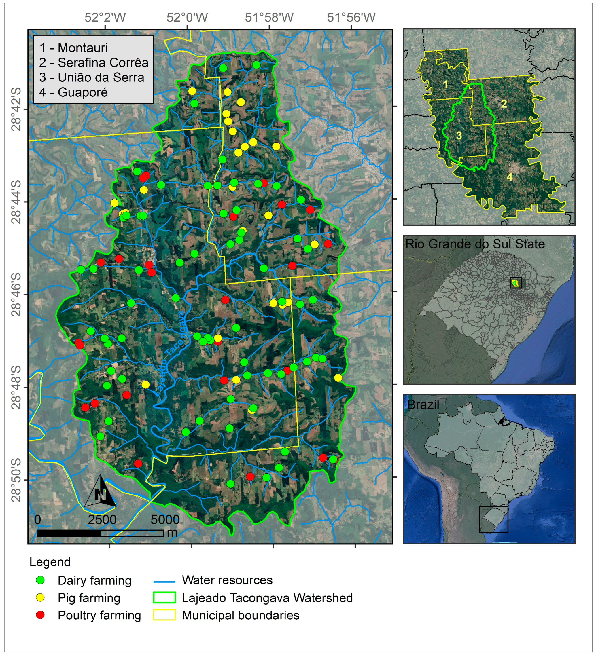
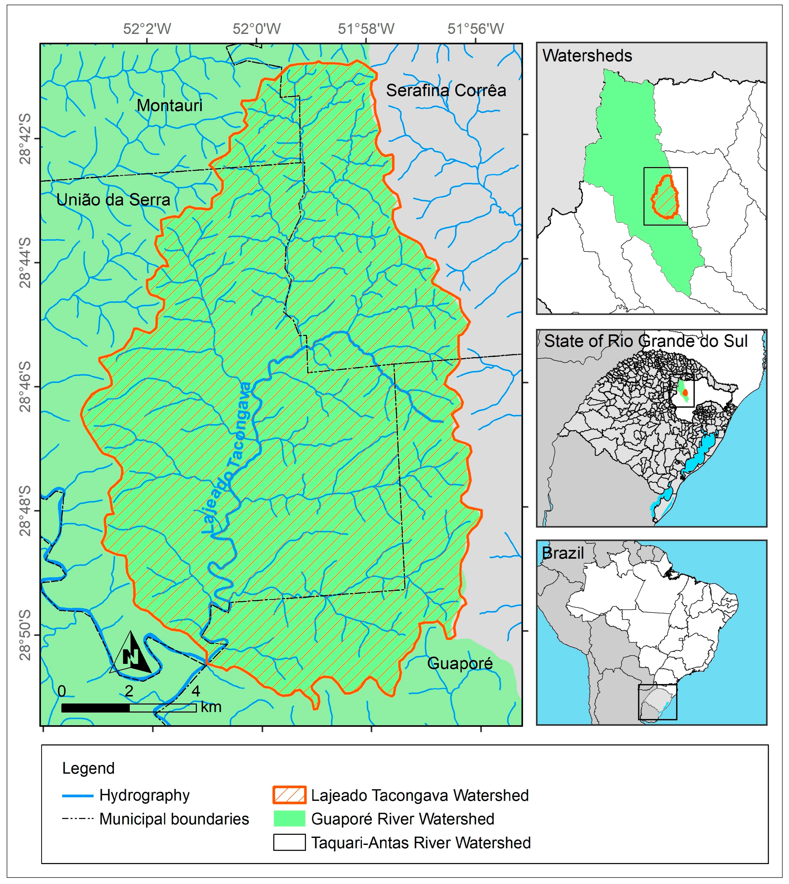
2.1. Study Area

The Lajeado Tacongava watershed (150 km²) is located in the northeast region of Rio Grande do Sul State, Southern Brazil, in the Middle Guaporé River within the Taquari-Antas basin (26,430 km²), as shown in Figure 1.

The study area comprises the partial territory of four cities (Guaporé, Serafina Correa, União da Serra, Montauri). For the year 2018, 115 farms with broiler, pig, and dairy productions were identified within the watershed (Figure 2).

2.2. Input Data

2.2.1. Human Water Consumption (HWC) and Livestock Water Consumption (LWC)

The HWC refers to the water consumption by each water use (sector), such as domestic, livestock, irrigation, and industry. Water consumption is a form of water use and is defined as the amount of water removed from, but not returned to, the same drainage basin [15]. In this study, the HWC comprises livestock water consumption (LWC) and domestic water consumption (DWC). No other water uses were identified within the watershed in the study year.

LWC refers to the technical water (drinking, cleaning, and cooling) consumed by livestock production in 2018. It was calculated monthly for each farm assessed. Water consumption for pig and poultry drinking [26], cleaning [27], and the poultry cooling system [28] was calculated considering a fraction of water consumption per head, as presented by Carra et al. [29]. In dairy production systems, milk yield, diet features, and temperature were considered to calculate water consumption for animal drinking [30], while cleaning water consumption was calculated considering the daily amount of water per head of cattle based on the literature [31], and water consumption for the cooling system for confined farms was considered as presented by Carra et al. [32].

DWC refers to water consumed to meet human demands. It was calculated considering the population within the watershed and the mean water consumption of 125 L hab⁻¹ day⁻¹ as proposed by the Brazilian Water Agency for rural areas in Southern Brazil with a deduction of 80% regarding the water fraction that returns to the water body [33]. The population in the watershed was estimated at 1802 inhabitants through the rural demographic density (hab.km⁻¹) considering the rural area (km²). The rural population and the area of each municipality within the watershed were based on the latest agricultural census [34].

2.2.2. Water Availability (WA)

Water availability is defined by ISO 14046 [35] as the extent to which humans and ecosystems have sufficient water resources for their needs. In this study, the applied methods consider different concepts of WA but both use the natural runoff. The natural runoff was calculated as the long-term water daily average, or the runoff, considering data recorded by a gauge station, code: 86560000, located downstream of the study area, in the Guaporé River watershed mouth. It is part of the Brazilian hydrological monitoring network system HidroWeb managed by the Brazilian Water Agency. A database for 79 years (1939–2018) was considered [36]. The river basin area at the gauge station is 2030 km²; therefore, data were regionalized for the watershed area (150 km²) by the ration between the drainage areas. In scenarios SC.3 and SC.4 (Table 1), lower WA following the concept used by the methods applied (see Section 2.3) was analyzed with Q₉₀ and Q₈₀ as WA, i.e., the runoff is greater than or equal to 90% and 80% of the time, respectively. In scenario SC.5 (Table 1), the WA was considered Q₉₅ as defined by the Brazilian Water Agency [11].

2.2.3. Environmental Water Requirement (EWR)

The EWR refers to the amount of water to sustain ecosystems [37]. In this study, the EWR refers to surface water. In the Taquari-Antas basin (Figure 1), the hydrographic basin plan [38] defines the EWR (m² s⁻¹ month⁻¹) as Q₉₅, as considered in scenarios SC.2; SC.3; SC.4 (Table 1). The water reference flow was calculated based on daily average data for 79 years (1939–2018) recorded by the same gauge station (see Section 2.2.2) located at the mouth of Guaporé River. Data from the gauge station were transferred to the study area by flow regionalization, obtaining the permanence curve for the study area. From the permanence curve, the daily reference flow data for the basin was obtained, as well as the Q₉₀ and Q₈₀ considered as WA in scenarios SC.3 and SC.4 (Table 1), respectively.

In the AWARE method, Boulay et al. [39] recommend calculating the EWR according to Pastor et al. [37], who propose a fraction of EWR between 30% and 60%, depending on the WA. Therefore, the EWR ranges throughout the year following the runoff hydrograph. Hoekstra et al. [16] suggest considering a constant EWR of 80% of runoff throughout the year based on the WA, following Richter et al. [40]. These definitions from the methods were applied in scenario SC.1 (Table 1). In scenario SC.5 (Table 1), the authors assumed half of Q₉₅ (50%Q₉₅) as EWR to evaluate the behavior of water scarcity with even lower EWR.

2.3. Water Scarcity Impact Assessment

The methods available water remaining (AWARE) [39] and the blue scarcity water index (BWSI) [16] were applied for the water scarcity impact assessment in the study area considering monthly data on human water consumption (HWC), environmental water requirement (EWR), and surface water availability (WA).

2.3.1. Water Available Remaining (AWARE)

The method is based on the quantification of the available water remaining (AMDi; availability minus demand) per watershed area (Area; m²) once the HWC (m³ month⁻¹) and EWR (m³ month⁻¹) have been met considering the WA (m³ month⁻¹) [39]. The AWARE method considers WA as the natural runoff. The AMDi (m³ m⁻² month⁻¹) was calculated monthly following the Equation (1).

$${\mathrm{A}\mathrm{M}\mathrm{D}}_{\mathrm{i}}=\frac{\mathrm{W}\mathrm{A}-\mathrm{H}\mathrm{W}\mathrm{C}-\mathrm{E}\mathrm{W}\mathrm{R}}{\mathrm{A}\mathrm{r}\mathrm{e}\mathrm{a}}$$

(1)

The characterization factor CF_AWARE (Equation (2)) expresses the impact score value of AMDi compared to the world’s average AMDworld.avg (0.0136 m³ m⁻² month⁻¹). CF_AWARE is expressed in m³ world eq.m⁻³, and the water scarcity ranges from 0.1 (minimum) to 100 (maximum) [39].

$${\mathrm{C}\mathrm{F}}_{\mathrm{A}\mathrm{W}\mathrm{A}\mathrm{R}\mathrm{E}}=\frac{\mathrm{A}\mathrm{M}\mathrm{D}\mathrm{w}\mathrm{o}\mathrm{r}\mathrm{l}\mathrm{d}.\mathrm{a}\mathrm{v}\mathrm{g}}{{\mathrm{A}\mathrm{M}\mathrm{D}}_{\mathrm{i}}}$$

(2)

The water scarcity footprint (WSF), which quantifies the potential environmental impact related to water scarcity [15] associated with livestock production, was calculated by multiplying the LWC in the watershed by the monthly CF_AWARE [35], following Equation (3), converting the consumed water into a reference equivalent [41]. WSF is presented in m³ world eq./t output.

$$\mathrm{W}\mathrm{S}\mathrm{F}=\mathrm{L}\mathrm{W}\mathrm{C}\ast {\mathrm{C}\mathrm{F}}_{\mathrm{A}\mathrm{W}\mathrm{A}\mathrm{R}\mathrm{E}}$$

(3)

2.3.2. Blue Water Scarcity Index (BWSI)

Hoekstra et al. [42] defined blue water scarcity in a river basin as the ratio of the total blue water consumption to the blue water availability in a river basin during a specific time period. The BWSI is calculated as presented in Equation (4) as the ratio of the HWC (m³ month⁻¹) in a watershed to the WA (m³ month⁻¹), where the latter subtracts the EWR (m³ month⁻¹) [16]. The WA is considered as natural runoff plus HWC [42]

$$\mathrm{B}\mathrm{W}\mathrm{S}\mathrm{I}=\frac{\mathrm{H}\mathrm{W}\mathrm{C}}{\mathrm{W}\mathrm{A}-\mathrm{E}\mathrm{W}\mathrm{R}}$$

(4)

BWSI is without unit and results are presented in percentage of the total water consumption (%). The original approach uses BWSI to identify water use in processes in regions where local consumption violates EWR (BWSI > 1) [15]. Therefore, the same reference suggests presenting the results in terms of CF, with CF_BWSI of 0 when BWSI < 1 or CF_BWSI of 1 when BWSI > 1 (binary approach). BWSI was calculated considering HWC, and the percentage of LWC contribution to water scarcity is indicated. The method proposes four classifications of water scarcity level: low (BWSI < 1); moderate (1.0 < BWSI < 1.5); significant (1.5 < BWSI < 2.0); and severe (WS > 2.0) [43].

2.4. Scenario Settings

Five scenarios were set (Table 1) to calculate the local CF_AWARE and BWSI to assess the impact of livestock production on water scarcity using different WA and EWR input data, including national and local regulations and definitions from the literature, as presented in Section 2.2.2 and Section 2.2.3. This ensures the comparability of results with other studies and allows for the discussion of potential scenarios with lower water flows. The HWC was constant for all scenarios assessed.

Table 1. Scenario set to assess the local CF_AWARE and BWSI in the study area.

Scenarios	WA				HWC	EWR
	Runoff *	Q95	Q90	Q80		Q95	50% Q95	Pastor et al. [39]	Richter et al. [41]
SC.1_AWARE	x				x			x
SC.2_AWARE	x				x	x
SC.3_AWARE			x		x	x
SC.4_AWARE				x	x	x
SC.5_AWARE		x			x		x
SC.1_BWSI	x				x				x
SC.2_BWSI	x				x	x
SC.3_BWSI			x		x	x
SC.4_BWSI				x	x	x
SC.5_BWSI		x			x		x

Notes: WA: water availability; HWC: human water consumption (LWC + DWC); EWR: environmental water requirement. * In the AWARE method, WA was considered as natural runoff, in the BWSI method, WA was considered as natural runoff plus HWC.

Table 1. Scenario set to assess the local CF_AWARE and BWSI in the study area.

Scenarios	WA				HWC	EWR
	Runoff *	Q95	Q90	Q80		Q95	50% Q95	Pastor et al. [39]	Richter et al. [41]
SC.1_AWARE	x				x			x
SC.2_AWARE	x				x	x
SC.3_AWARE			x		x	x
SC.4_AWARE				x	x	x
SC.5_AWARE		x			x		x
SC.1_BWSI	x				x				x
SC.2_BWSI	x				x	x
SC.3_BWSI			x		x	x
SC.4_BWSI				x	x	x
SC.5_BWSI		x			x		x

Notes: WA: water availability; HWC: human water consumption (LWC + DWC); EWR: environmental water requirement. * In the AWARE method, WA was considered as natural runoff, in the BWSI method, WA was considered as natural runoff plus HWC.

Quantitative data uncertainty was assessed through descriptive statistical analysis (e.g., average values, standard deviation, coefficient of variation), while qualitative uncertainties are discussed throughout the study.

3. Results and Discussion

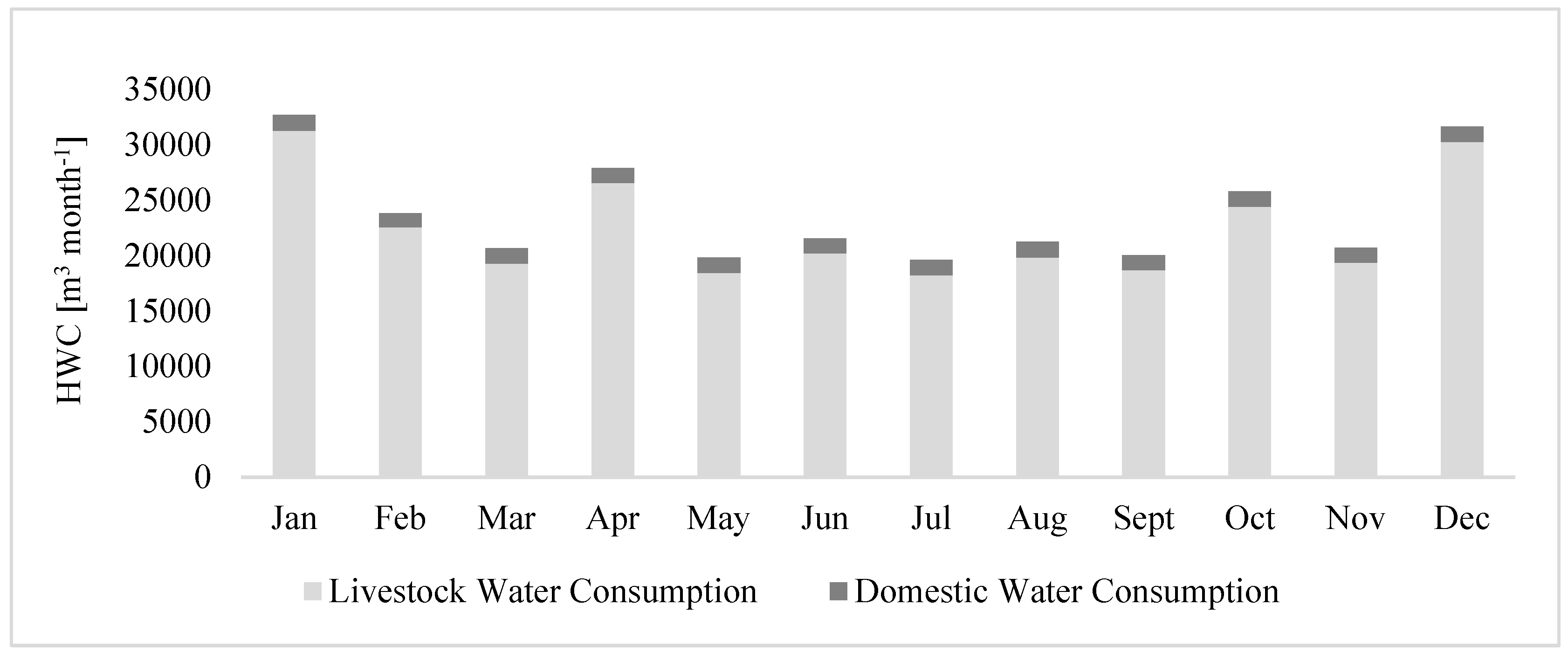
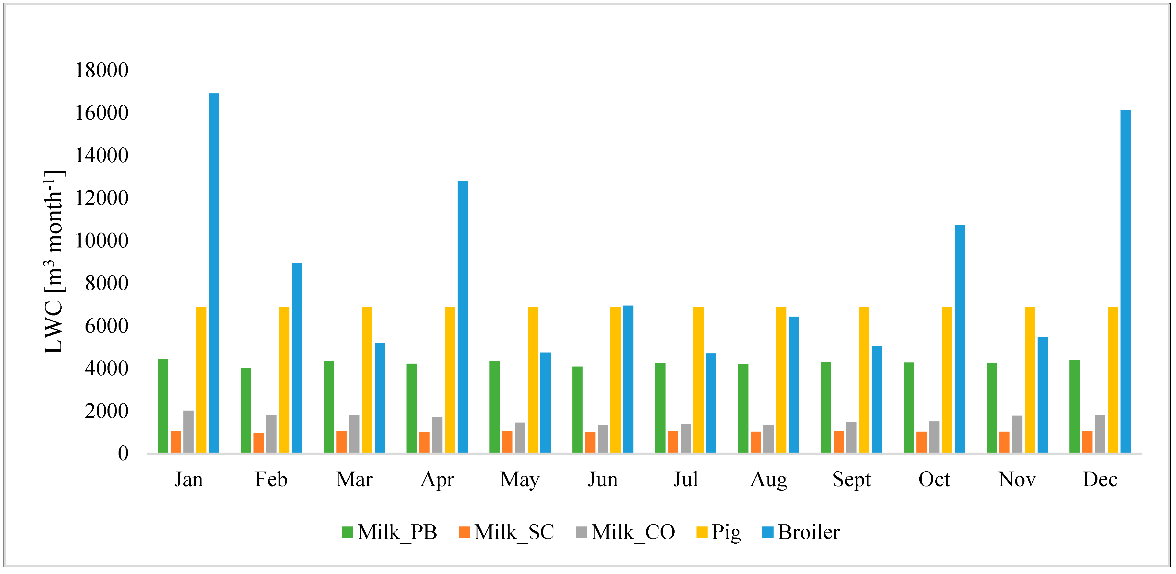
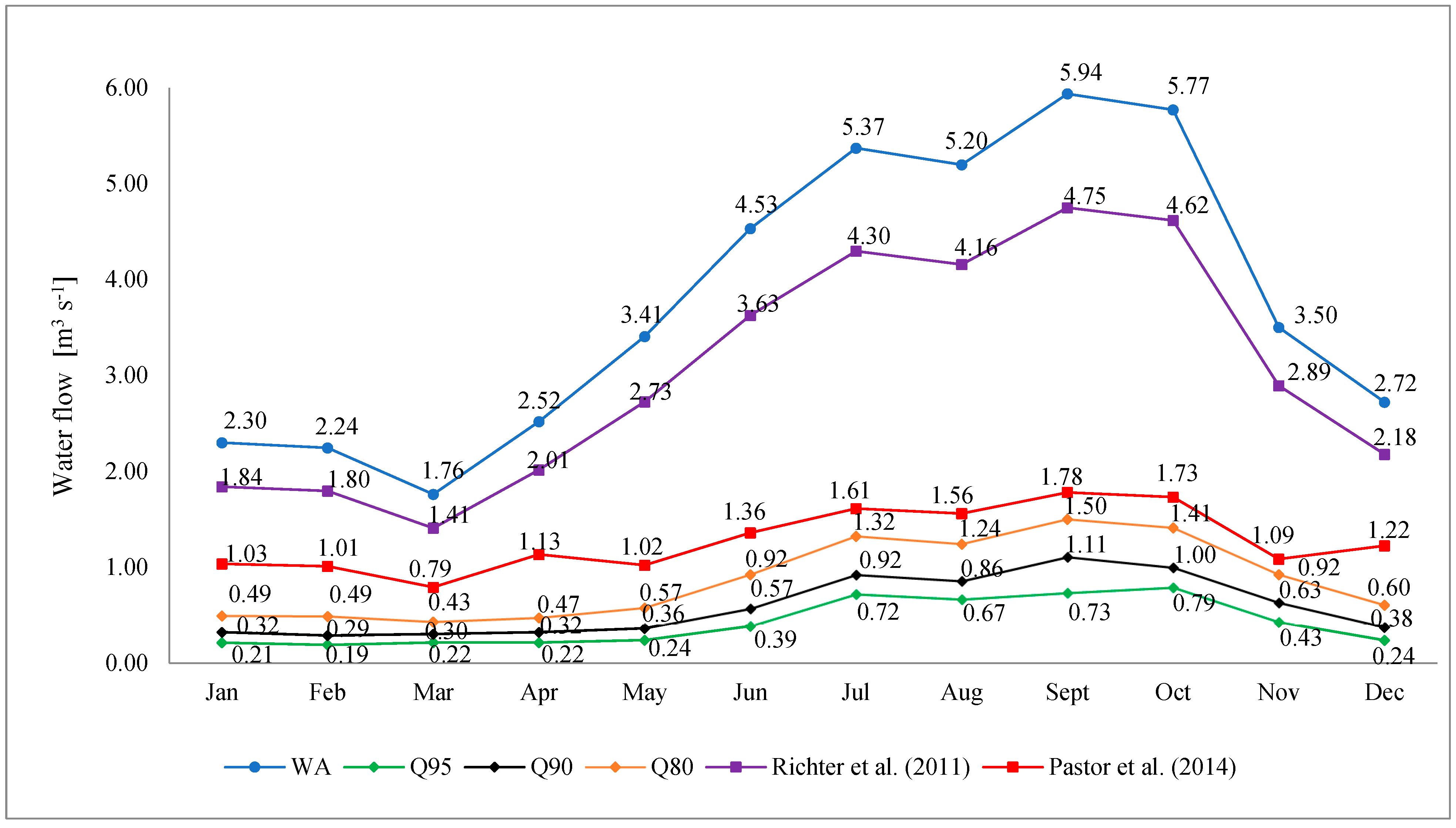
3.1. Monthly HWC, EWR and WA

The HWC (285,514 m³ year⁻¹) was mainly composed of LWC (94%) with an average of 22,422 m³ month⁻¹ ± 4462 SD (standard deviation) followed by DWC (6.0%) with an average of 1371 m³ month⁻¹ ± 38.8 SD. The monthly results of total water consumption throughout the year are shown in Figure 3.

The DWC remained constant throughout the year, while the LWC increased during the summer months when temperatures were higher, particularly in January (average of 21.4 °C ± 3.8 SD) and December (average of 20.8 °C ± 5.7) [44], as presented in

Table 2. Technical water consumed (m³ month⁻¹) by livestock (LWC) in the study area in 2018 [29,32].

Technical Water Use	Jan	Feb	Mar	Apr	May	Jun	Jul	Aug	Sept	Oct	Nov	Dec
Drinking	13,404	12,898	13,329	13,154	13,321	12,993	13,203	13,136	13,254	13,216	13,201	13,373
Cleaning	4760	4760	4760	4760	4760	4760	4760	4760	4760	4760	4760	4760
Cooling	13,099	4918	1173	8653	365	2446	245	1946	672	6433	1404	12,109
Total	31,263	22,576	19,263	26,567	18,446	20,199	18,209	19,842	18,686	24,409	19,365	30,242

. The cooling system used in poultry and confined milk production systems is activated after reaching a specific temperature [29,32], and the water intake of lactating cows is influenced by minimum temperature, in addition to other aspects (e.g., dry matter and sodium intake and milk yield). Drinking water represented 58.8% of LWC, while cleaning and cooling accounted for 21.3% and 19.9%, respectively.

Figure 4 presents the LWC for each animal production system throughout the year. Poultry production presented the highest annual water consumption (38.7%), followed by pig (30.7%) and milk production (30.6%).

Among farmers interviewed, almost 73% reported using groundwater to supply livestock and domestic water needs. Therefore, technical water consumed on the farms assessed was withdrawn mainly from the fractured aquifer located over the study area. According to Reginato and Strieder [45], more than 90% of the Taquari-Antas basin is over a fractured aquifer called Sistema Aquifero Serra Geral (SASG). It presents an intense variation in the annual flow that can be exploited from the aquifer without having an undesirable effect [46]. The characteristics of the aquifer and the lack of data to assess its potential recharge confer a high uncertainty to estimate the groundwater recharge effective contribution to the study area as WA. In addition, quantifying the amount of groundwater used for livestock production in the study area is also highly uncertain. This is because most farmers do not have any equipment to measure water withdrawal; reporting to the state government estimates based on their daily work experience, or with the support of technicians who use technical references from the literature.

Therefore, despite the predominance of groundwater use in the study area, a distinction between water sources was not considered in this study, following the recommendations of Boulay et al. [47] to avoid higher uncertainties. The authors recognize that looking at the stress on surface and groundwater separately might be desirable, but give several reasons for assessing the overall pressure on the water resource by providing only one generic indicator from an unspecified water source. Among the reasons pointed out by the authors and clearly observed in the study area is the lack of reliable data on groundwater uses and the need for robust knowledge of the interaction between surface, groundwater, and ecosystems considering the characteristics of the aquifers.

Figure 5 presents the WA and the statistical low-flow Q₉₅, Q₉₀ and Q₈₀ besides the EWR calculated according to Pasture et al. [37] and Richter et al. [40]. The WA was almost the same for AWARE (annual average: 3.77 m³s⁻¹) and BWSI (annual average: 3.78 m³s⁻¹) due to the low HWC (annual average: 0.108 m³s⁻¹ ± 0.00176 SD). The monthly average precipitation was 135 mm ± 51 SD and 172 mm ± 33 SD in summer, from January to April, and in the last year’s quarter, and winter, from May to September, respectively [44]. Considering the technical water consumption was higher in summer, as already explained, higher water flows were observed in the winter season.

The WA (AWARE, BWSI) in SC.1, and SC.2 presented an annual average flow of 3.78 m³ s⁻¹ ± 1.4 SD. The Q₉₅ considered as WA in SC.5 and as EWR in SC.1, SC.3, and SC.4 presented an annual average flow of 0.42 m³ s⁻¹ ± 0.23 SD. The Q₉₀ and Q₈₀ considered as WA in SC.3, and SC.4 presented an annual average flow of 0.59 m³ s⁻¹ ± 0.29 SD and 0.87 m³ s⁻¹ ± 0.39 SD, respectively. In SC.2_BWSI, the EWR following Richter et al. [40] presented an annual average flow of 3.03 m³ s⁻¹ ± 1.2 SD, which was more than double of the EWR found following Pastor et al. (2014), employed in SC.2_AWARE (annual average flow of 1.28 m³ s⁻¹ ± 0.31 SD).

3.2. Water Scarcity Impact Assessment

Table 3. Water scarcity impact assessment (AWARE; BWSI) associated with livestock production per ton of output in the study area in 2018.

			Jan	Feb	Mar	Apr	May	Jun	Jul	Aug	Sept	Oct	Nov	Dec	Mean
Inventory results Water consumption [m3/product]	Poultry [m3/t CW]	Drinking	4.1	4.1	4.1	4.1	4.1	4.1	4.1	4.1	4.1	4.1	4.1	4.1	4.1
		Cleaning	0.0	0.0	0.0	0.0	0.0	0.0	0.0	0.0	0.0	0.0	0.0	0.0	0.0
		Cooling	11.2	4.0	0.6	7.5	0.2	2.2	0.1	1.7	0.4	5.6	0.8	10.5	3.7
		Total	15.4	8.1	4.7	11.6	4.3	6.3	4.3	5.9	4.6	9.8	5.0	14.7	7.9
	Pig [m3/t CW]	Drinking	6.9	6.9	6.9	6.9	6.9	6.9	6.9	6.9	6.9	6.9	6.9	6.9	6.9
		Cleaning	8.5	8.5	8.5	8.5	8.5	8.5	8.5	8.5	8.5	8.5	8.5	8.5	8.5
		Total	15.4	15.4	15.4	15.4	15.4	15.4	15.4	15.4	15.4	15.4	15.4	15.4	15.4
	Milk_PB [m3/t FPCM]	Drinking	8.4	7.5	8.3	8.0	6.7	6.2	6.5	6.4	6.6	8.1	8.1	8.4	7.4
		Cleaning	1.5	1.5	1.5	1.5	1.2	1.2	1.2	1.2	1.2	1.5	1.5	1.5	1.4
		Total	9.9	9.0	9.8	9.5	7.9	7.4	7.7	7.6	7.8	9.6	9.6	9.9	8.8
	Milk_SC [m3/t FPCM]	Drinking	7.5	6.7	7.4	7.1	5.9	5.5	5.8	5.7	5.8	7.2	7.2	7.5	6.6
		Cleaning	1.2	1.2	1.2	1.2	0.9	0.9	0.9	0.9	0.9	1.2	1.2	1.2	1.1
		Total	8.7	7.9	8.6	8.3	6.9	6.4	6.7	6.6	6.8	8.4	8.4	8.7	7.7
	Milk_CO [m3/t FPCM]	Drinking	5.7	5.7	5.7	5.7	5.7	5.7	5.7	5.7	5.7	5.7	5.7	5.7	5.7
		Cleaning	0.9	0.9	0.9	0.9	0.9	0.9	0.9	0.9	0.9	0.9	0.9	0.9	0.9
		Cooling	3.9	2.8	2.8	2.3	0.9	0.3	0.5	0.4	1.0	1.3	2.7	2.8	1.8
		Total	10.5	9.4	9.4	8.8	7.5	6.9	7.1	7.0	7.6	7.9	9.2	9.4	8.4
Scarcity footprint [m3 world eq./t output] Boulay et al. [17]	SC.1 AWARE	CFAWARE *	0.61	0.69	0.79	0.57	0.32	0.25	0.20	0.21	0.19	0.19	0.31	0.51	0.4
		Poultry	9.4	5.6	3.7	6.7	1.4	1.6	0.9	1.2	0.9	1.8	1.5	7.5	3.5
		Pig	9.4	10.6	12.2	8.8	4.9	3.8	3.1	3.2	2.9	2.9	4.8	7.9	6.2
		Milk_PB	6.0	6.2	7.8	5.4	2.5	1.8	1.6	1.6	1.5	1.8	3.0	5.1	3.7
		Milk_SC	5.3	5.4	6.8	4.8	2.2	1.6	1.4	1.4	1.3	1.6	2.6	4.4	3.2
		Milk_CO	6.4	6.5	7.4	5.1	2.4	1.7	1.4	1.5	1.4	1.5	2.9	4.8	3.6
	SC.2 AWARE	CFAWARE *	0.37	0.41	0.50	0.34	0.24	0.19	0.16	0.17	0.15	0.15	0.25	0.31	0.3
		Poultry	5.6	3.4	2.3	4.0	1.0	1.2	0.7	1.0	0.7	1.5	1.2	4.5	2.3
		Pig	5.7	6.4	7.6	5.3	3.7	2.9	2.5	2.6	2.3	2.4	3.8	4.8	4.2
		Milk_PB	3.6	3.7	4.8	3.3	1.9	1.4	1.3	1.3	1.2	1.5	2.4	3.0	2.4
		Milk_SC	3.2	3.3	4.3	2.9	1.7	1.2	1.1	1.1	1.0	1.3	2.1	2.7	2.1
		Milk_CO	3.9	3.9	4.6	3.0	1.8	1.3	1.2	1.2	1.1	1.2	2.3	2.9	2.4
	SC.3 AWARE	CFAWARE *	7.8	9.7	9.4	8.2	6.6	4.5	3.9	4.2	2.1	3.9	4.0	6.0	5.9
		Poultry	119.7	78.9	44.4	95.0	28.5	28.4	16.6	24.5	9.8	37.8	19.9	88.5	49.3
		Pig	120.0	149.6	145.1	126.0	101.9	69.4	59.7	64.6	33.1	59.5	61.9	93.0	90.3
		Milk_PB	77.2	87.4	92.1	77.3	52.2	33.4	29.9	31.9	16.8	37.0	38.4	59.5	52.7
		Milk_SC	67.7	76.6	80.8	67.9	45.3	29.0	26.0	27.8	14.5	32.5	33.7	52.2	46.2
		Milk_CO	81.7	90.9	88.3	72.2	49.6	31.0	27.5	29.2	16.3	30.3	37.1	56.6	50.9
	SC.4 AWARE	CFAWARE *	2.8	3.0	3.7	3.2	2.3	1.5	1.3	1.3	1.0	1.2	1.6	2.1	2.1
		Poultry	43.8	24.0	17.5	37.4	10.0	9.4	5.5	7.9	4.8	12.2	8.0	31.5	17.7
		Pig	43.9	45.5	57.1	49.6	35.9	23.0	19.7	20.7	16.0	19.2	24.9	33.0	32.4
		Milk_PB	28.2	26.6	36.2	30.4	18.4	11.0	9.9	10.3	8.1	11.9	15.4	21.1	19.0
		Milk_SC	24.8	23.3	31.8	26.7	16.0	9.6	8.6	8.9	7.0	10.5	13.5	18.6	16.6
		Milk_CO	29.9	27.7	34.7	28.4	17.5	10.3	9.1	9.4	7.9	9.8	14.9	20.1	18.3
	SC.5 AWARE	CFAWARE *	8.1	9.8	7.6	8.1	6.8	4.2	2.2	2.3	2.2	2.0	3.8	7.1	5.4
		Poultry	124.9	79.9	36.1	94.6	29.2	26.8	9.2	13.7	10.0	19.3	18.9	104.7	47.3
		Pig	125.2	151.5	117.7	125.5	104.3	65.5	33.3	36.1	33.8	30.5	58.8	110.0	82.7
		Milk_PB	80.5	88.5	74.7	77.0	53.4	31.5	16.7	17.8	17.1	18.9	36.5	70.4	48.6
		Milk_SC	70.7	77.6	65.6	67.6	46.4	27.4	14.5	15.5	14.8	16.6	32.0	61.8	42.5
		Milk_CO	85.2	92.1	71.6	71.9	50.8	29.3	15.3	16.3	16.6	15.5	35.3	67.0	47.2
Scarcity factor BWSI Hoekstra et al. [18]	BWSI Binary (0 or 1) **		0	0	0	0	0	0	0	0	0	0	0	0
	BWSI (%)	SC.1	2.7	2.2	2.2	2.1	1.1	0.9	0.7	0.8	0.7	0.8	1.1	2.2	1.4
		SC.2	0.6	0.5	0.5	0.5	0.2	0.2	0.2	0.2	0.1	0.2	0.3	0.5	0.3
		SC.3	11.1	10.2	8.7	10.1	6.0	4.5	3.6	4.2	2.1	4.7	3.9	8.5	6.5
		SC.4	4.4	3.3	3.6	4.2	2.2	1.5	1.2	1.4	1.0	1.6	1.6	3.2	2.4
		SC.5	11.5	10.3	7.2	10.0	6.2	4.3	2.0	2.4	2.1	2.4	3.7	10.0	6.0
	Contribution of livestock production to water scarcity		96%	95%	93%	95%	93%	94%	93%	93%	93%	95%	93%	96%	94%
	Contribution (%) of each livestock production to water scarcity *	Poultry	54%	40%	27%	48%	26%	35%	26%	33%	27%	44%	28%	53%	37%
		Pig	22%	31%	36%	26%	37%	34%	38%	35%	37%	28%	36%	23%	32%
		Milk_PB	14%	18%	23%	16%	24%	20%	23%	21%	23%	18%	22%	15%	20%
		Milk_SC	3%	4%	5%	4%	6%	5%	6%	5%	6%	4%	5%	4%	5%
		Milk_CO	7%	8%	9%	6%	8%	6%	7%	6%	8%	6%	9%	6%	7%

Notes: Milk_PB: milk produced in pasture-based system; Milk_SC: milk produced in semi-confined system; Milk_CO: milk produced in confined system; CW: carcass weight; SD: standard deviation; * CF_AWARE [m³ world eq/m³ water used]; ** BWSI = 0 in all scenarios assessed.

presents the CF_AWARE and CF_BWSI and the water scarcity impact assessment associated with livestock production considering the amount of water consumed (m³) to produce 1 ton (t) of animal product (carcass weight of pig; carcass weight of poultry, fat protein corrected milk) following the recommendations of the FAO [15].

According to Boulay et al. [39], a CF_AWARE value of 1 m³ world eq/m³ water used indicate regions with the same amount of remaining water per area in a certain period of time as the world average; a value of CF < 1 m³ world eq/m³ water used indicate regions with lower water scarcity than the world average; and a value of 10 m³ world eq/m³ water used, for example, indicate a region where there is 10 times less water remaining per area in a certain period of time compared to the world average. Based on these definitions, results observed in SC.1_AWARE and SC.2_AWARE demonstrate lower water scarcity in the study area than the world average in all months. The highest local CF_AWARE among scenarios assessed observed in February in SC.5 (9.82 m³ world eq/m³ water used) and SC.3 (9.69 m³ world eq/m³ water used) demonstrate the study area has almost 10 times less water remaining per area than the world average in drier water flow conditions.

Despite a contribution of more than 93% of livestock production to water scarcity throughout the year, the scarcity index indicator CF_BWSI was lower than 1 in all months, demonstrating the water consumption and the EWR do not exceed WA. Results indicate a low blue water scarcity considering all water consumption (HWC) throughout the year. Hoekstra et al. [16] assessed the monthly BWSI in some global hydrographic units, including the Uruguai hydrographic unit (365,000 km²) that partially comprises the Rio Grande do Sul State territory. Results reported by Hoekstra et al. [16] presented a correlation of R = 0.74 with results found in scenario SC.1_BWSI and both studies reported higher water scarcity in the first and fourth year quarter.

The first and fourth year quarter, the summer season, presented the highest water scarcity according to both methods assessed due to the lower WA and higher LWC, mainly in February and March in all scenarios. The coefficient of variation of CF_AWARE and BWSI was higher than 40.3% and 45.6%, respectively, throughout the year with the highest variation in SC.1 of 51.7% and 49.5%. Among scenarios assessed, the highest CF_AWARE and BWSI were observed in a drier flow condition in SC.3 (WA = Q₉₀) with an annual average of 5.86 m³ eq/m³ water used ± 2.36 SD and 6.45% ± 2.94 SD, respectively. Results cannot be neglected considering the return period of Q₉₀ of two years.

Results of CF_AWARE in SC1 present a strong correlation of R = 0.94 and R = 0.99 and similar behavior throughout the year with those found in other studies carried out in the Taquari-Antas [20] basin and the South Atlantic hydrographic [39], respectively, which considered similar data input sources for WA and EWR. As recommended by Boulay et al. [39], the quantification of water scarcity should prioritize data on a monthly scale at a watershed level to result in more accurate water scarcity indicators. Results of CF_AWARE reported by Andrade et al. [20] indicated higher scarcity than local CF_AWARE found in this study, with differences greater than 23.5% and the largest observed in November (57.4%). The same comparison with CF_AWARE reported by Boulay et al. [39] showed lower water scarcity in more than half of the months, mainly in summer, than local CF_AWARE.

Regarding the impact of water scarcity associated with livestock production, pig production presented the highest water consumption per output throughout the year and, consequently, the highest WSF. Under a low water flow condition (SC.3), the potential impact of consuming 15.4 m³ to produce 1 ton of pig CW in the study area is equivalent to a consumption of an annual average of 90.3 m³ ± 36.3 SD in a world average area considering 5.9 times less remaining water than the world average (annual average CF_AWARE = 5.9 m³ world eq/m³ water used ± 2.4 SD, Table 3). Considering the same drier flow scenario (SC.3), WSF of pig CW is 14.5 times greater than in SC.1. In scenarios SC.3 and SC.5, the first and fourth year quarter, when water flow is lower and LWC is higher, presented the highest WSF for all animal production in the watershed (Table 3).

Among milk production systems, milk produced in pasture-based system presented the highest WSF, with the highest annual average results obtained in SC.3 (52.7 m³ world eq./t FPCM ± 24.3 SD). It was 12.4% and 3.5% higher than the annual average WSF of milk produced in semi-confined and confined systems in the same scenario, respectively. In Australia, Ridoutt et al. [23] applied the AWARE method to assess the WSF of dairy milk produced in 75 pasture-based farms and found a wide variation of results ranging from 17.6 to 28,769 m³ world eq./t FPCM. Payen et al. [22] reported a WSF of 22 L world eq/kg FPCM and 1118 L world eq/kg FPCM for milk and meat produced in pasture-based farms in two regions in New Zealand. The WSF of milk produced in Finland was assessed by Usva et al. [21] that reported 12.2 l eq. l⁻¹ skimmed milk. Despite the differences in the study year, production systems, outputs, units, and other features that do not allow the comparison among results of the mentioned studies, they demonstrate the scientific concern of assessing WSF of animal production. In Brazil, Palhares and Perpezonne [25] applied the BWSI method in an organic farm and a conventional dairy farm and reported similar water scarcity index results as found in this study (SC.3), of 13% and 11%, respectively.

Poultry production also presented the highest WSF in SC.3, with an annual average of 49.3 m³ world eq./t CW ± 34.9 SD and higher water scarcity in summer, mainly in January (119.7 m³ world eq./t CW) and the lowest in September (9.8 m³ world eq./t CW). The annual average WSF for poultry production in SC.3 was 14 times greater than in SC.1 (3.5 m³ world eq./t CW) and 69% greater than in SC.5 (29.1 m³ world eq./t CW). In Australia, Copley and Wiedemann [48] assessed AWARE in conventional (WSF of 23.1 m³ ± 1.7 SD) and free-range poultry meat (24.5 m³ ± 2.2 SD), considering water consumption for animal production and meat processing. The authors found a contribution of breeding operations to water scarcity of 6%.

Despite the unalarming water scarcity observed in the watershed in both methods applied, it demonstrates the importance of adopting best practices to improve water productivity, and reducing the risks of potential production losses considering the projections of the Brazilian Water Agency [11] and more regular severe drought projection [9], mainly in low water flow periods. Several best practices are pointed out by Palhares [49] for a more sustainable water use on dairy farms, considering the characteristics of milk production in Brazil. De Avila et al. [50] and Souza et al. [51] present best practices to improve water performance in poultry and pig productions in Brazil.

In the study area, the great amount of annual precipitation and its good distribution during the year meet the agricultural demands. Therefore, no irrigation was observed in the watershed in the study year and rainfed crops and pasture are used to feed the animals. For this reason, most farmers do not have irrigation systems. Although pasture irrigation for milk production is being used by 6.28% of farmers in Rio Grande do Sul State, it has increased by 42.4% since 2015 [52]. Hence, the consumption of blue water is expected to expand in the next years in Rio Grande do Sul State increasing the potential of scarcity in the near future. This is some critical piece of information for decision-makers to take into account. Therefore, further studies on the assessment of water scarcity in the Taquari-Antas basin considering climate change scenarios are recommended.

Although the local water scarcity results found in the study indicate a non-critical situation, the main source of water in this region, the groundwater, was not taken into account in the water scarcity impact assessment in this study, as previews mentioned. Gejl et al. [53] proposed and validated a modification of the AWARE method, AGWaRE (available groundwater remaining), in a study in Denmark to assess groundwater stress. The method takes into account the groundwater recharge as the water availability, the environmental groundwater requirement, and groundwater consumption. In another study, Lee et al. [54] used the AWARE method to quantify the water stress impact in the US, taking into account the groundwater recharge in areas where it was used. In both studies, the authors calculated a local AMDref rather than using a global reference. Therefore, more studies should be developed to contribute to this knowledge, improving water management in livestock production and supply chains, mainly in areas that rely on groundwater as in this study.

Besides groundwater, the integration of green water to the water scarcity impact assessment is also a challenge. As reported in the previous studies that present the assessment of water consumption (monthly) and water productivity of poultry and pig [29] and milk [32] in the study area, green water accounted for more than 99% of the total water consumption on farms assessed. Despite the representativeness of green water consumption, it was not accounted for in the water scarcity assessment in this study following the recommendations of the methods applied. Hoekstra et al. [16] highlight the BWSI is focused on blue water, and Boulay et al. [39] recommend addressing green water consumption linked with land use in a separate indicator [47]. Schyns et al. [55] reviewed and classified 80 indicators of green water availability and scarcity and concluded the concept of green water scarcity is still largely unexplored. According to the authors, to determine which part of the green water flow can be made productive in space and time, the difficulty of estimating green water consumption in some cases (e.g., forests) and the need for more research to determine the environmental green water requirements are the major challenges faced by green water scarcity indicators.

Data availability for the WSF assessment can be an issue when adopting a detailed geographic resolution. Intending to overcome this issue, Boulay et al. [39] recommend the aggregation of CF_AWARE for irrigation (CF agri) and for other sectors (CF non-agri) to country level and/or annual time step. For calculations based on the water consumption-weighted averages at the monthly and watershed scale, the aggregated factors should be used in regions with a lack of water flow data [39] as a constant factor throughout the year. Therefore, the WSF can be assessed for different sectors and products based on the aggregate CF_AWARE and water consumption.

Following this recommendation, Andrade et al. [20] and Bontinck et al. [19] calculated the aggregated CF for basins in Brazil and Australia, respectively. With the same purpose, CF_AWARE has been assessed for specific products, such as commodity-based products of mining industries [56] and for 26 crops’ typology at a national level for 224 countries [57], including wheat, corn, rice, soybean, and other. In Australia, Bontinck et al. [19] assessed an aggregated AWARE factor denominated CF non-irrigation, taking into account livestock drinking water, dairy, and piggery cleaning data. Kaewmai et al. [18] calculated the aggregated CFs for livestock and industry in a watershed in Thailand and the authors recommend the weighted average of AWARE CFs for each type of water consumption. No other studies were identified addressing aggregated CF_AWARE for livestock production.

In this study, under the condition of missing data of WA, the aggregated CF non-agri of 0.70 m³ world eq/m³ water used, reported by Andrade et al. [20] in the Taquari-Antas basin, could be used to assess WSF following the AWARE method. The comparison between WSF associated with animal production assessed based on local CF_AWARE, calculated in this study, and based on aggregated CF non-agri, reported by Andrade et al. [20], is shown in

Table 4. Water scarcity footprint (WSF) comparison using different CF_AWARE.

	local CFAWARE (SC.1) [m3 World eq/m3 Water Used]	CF Non-Agri Taquari-Antas Basin [m3 World eq/m3 Water Used]	Difference between the WSF (%)
Poultry	3.5	5.5	36.3
Pig	6.2	10.8	42.3
Milk_PB system	3.7	6.2	40.1
Milk_SC system	3.2	5.4	40.0
Milk_CO system	3.6	5.9	39.0

Note: SC.1: Scenario 1.

.

As observed in Table 4, the use of aggregated CF_AWARE non-agri presented an increase in WSF with a difference of results greater than 36.3% in comparison with WSF assessed based on local CF_AWARE. The difference in results can be associated with the calculation of the aggregated CF_AWARE non-agri, which took into account all water users (livestock, industry, domestic) except agriculture (irrigation), which has a specific aggregated CF_AWARE. Because of the low water scarcity observed in the study area, the difference between CF does not change the scenario. However, in watersheds with high water scarcity, this difference would reflect directly on the results.

For this reason, the calculation of an aggregated CF_AWARE taking into account livestock water consumption would support the assessment of WSF associated with animal production in regions where data on WA is not available, providing more accurate results and contributing to the water impact assessment in the sector. Considering scenarios of food production growth and the water demand for animal production, a close look at the livestock sector and its impacts on water scarcity could start with specific aggregated CF_AWARE for the sector. Even considering some challenges to have a special aggregated factor to livestock production because of the lack of data on livestock water consumption throughout the year, for example, the first step is to recognize its importance and to put effort to consider it in further studies.

4. Conclusions

Low water scarcity was observed in all scenarios assessed for both methods applied. Despite it being a non-alarming scenario, the insight gained from this study may support decision-makers, businesses, and farmers to make better decisions in the watershed. The study also provides knowledge for the livestock sector and for further studies, mainly those following the FAO LEAP guidelines.

Even considering different methods (inputs, concepts, and equations), results presented similar behavior of low water scarcity in the study area. More studies following the FAO LEAP guidelines with the application of the same methods for assessing water scarcity are encouraged to observe the behavior of the results. If other studies demonstrate similar water scarcity results from these methods, the application of only one method should be accepted and considered in a further edition of the FAO LEAP guidelines. Furthermore, due its binary approach, BWSI results are limiting for supporting decision-making. Therefore, it is recommended to apply other methods in parallel with AWARE. Further studies integrating groundwater availability are also encouraged.

The assessment of water scarcity supports water risk management and decision-making, and its application in livestock production is highly recommended, considering the expected growth of the sector, the dependency on water resources, and climate change. Studies should advance to integrate groundwater and green water to this assessment reducing the uncertainties and take into account climate change scenarios.

References

1. Xue, J.; Huo, Z.; Kisekka, I. Assessing Impacts of Climate Variability and Changing Cropping Patterns on Regional Evapotranspiration, Yield and Water Productivity in California’s San Joaquin Watershed. Agric. Water Manag. 2021, 250, 106852. [Google Scholar] [CrossRef]
2. FAO. The State of the World’s Land and Water Resources for Food and Agriculture—Systems at Breaking Point. Synthesis Report 2021; FAO: Rome, Italy, 2021. [Google Scholar] [CrossRef]
3. OECD/FAO. OECD-FAO Agricultural Outlook 2022–2031; 2022; Available online: https://www.oecd-ilibrary.org/agriculture-and-food/oecd-fao-agricultural-outlook-2022-2031_f1b0b29c-en (accessed on 23 October 2023). [CrossRef]
4. FAO and UN Water. Progress on Level of Water Stress. Global Status and Acceleration Needs for SDG Indicator 6.4.2; FAO: Rome, Italy, 2021. [Google Scholar] [CrossRef]
5. Boulay, A.M.; Drastig, K.; Chapagain, A.; Charlon, V.; Civit, B.; DeCamillis, C.; De Souza, M.; Hess, T.; Hoekstra, A.Y.; Ibidhi, R.; et al. Building Consensus on Water Use Assessment of Livestock Production Systems and Supply Chains: Outcome and Recommendations from the FAO LEAP Partnership. Ecol. Indic. 2021, 124, 107391. [Google Scholar] [CrossRef]
6. Weindl, I.; Bodirsky Benjamin, L.; Rolinski, S.; Biewald, A.; Lotze-Campen, H.; Müller, C.D. Livestock Production and the Water Challenge of Future Food Supply: Implications of Agricultural Management and Dietary Choices. Glob. Environ. Chang. 2017, 47, 121–132. [Google Scholar] [CrossRef]
7. Heinke, J.; Lannerstad, M.; Gerten, D.; Havlík, P.; Herrero, M.; Notenbaert, A.M.; Hoff, H.; Müller, C. Water Use in Global Livestock Production—Opportunities and Constraints for Increasing Water Productivity. Water Resour. Res. 2020, 56, e2019WR026995. [Google Scholar] [CrossRef]
8. Getirana, A. Extreme Water Deficit in Brazil Detected from Space. J. Hydrometeorol. 2016, 17, 591–599. [Google Scholar] [CrossRef]
9. Getirana, A.; Libonati, R.; Cataldi, M. Brazil Is in Water Crisis—It Needs a Drought Plan. Nature 2021, 600, 218–220. [Google Scholar] [CrossRef]
10. Agência Nacional de Águas (ANA). Conjuntura Dos Recursos Hídricos No Brasil 2021—Relatório Pleno; ANA: Brasília, Brazil, 2021. [Google Scholar]
11. Agência Nacional de Águas (ANA). National Water Security Plan; ANA: Brasília, Brazil, 2019. [Google Scholar]
12. Zhang, H.; Zhuo, L.; Xie, D.; Liu, Y.; Gao, J.; Wang, W.; Li, M.; Wu, A.; Wu, P. Water Footprints and Efficiencies of Ruminant Animals and Products in China over 2008–2017. J. Clean. Prod. 2022, 379, 134624. [Google Scholar] [CrossRef]
13. Richter, B.D.; Bartak, D.; Caldwell, P.; Davis, K.F.; Debaere, P.; Hoekstra, A.Y.; Li, T.; Marston, L.; McManamay, R.; Mekonnen, M.M.; et al. Water Scarcity and Fish Imperilment Driven by Beef Production. Nat. Sustain. 2020, 3, 319–328. [Google Scholar] [CrossRef]
14. Klopatek, S.C.; Oltjen, J.W. How Advances in Animal Efficiency and Management Have Affected Beef Cattle’s Water Intensity in the United States: 1991 Compared to 2019. J. Anim. Sci. 2022, 100, skac297. [Google Scholar] [CrossRef]
15. FAO (Food and Agriculture Organization). Water Use in Livestock Production Systems and Supply Chains—Guidelines for Assessment (Version 1); FAO: Rome, Italy, 2019. [Google Scholar]
16. Hoekstra, A.Y.; Mekonnen, M.M.; Chapagain, A.K.; Mathews, R.E.; Richter, B.D. Global Monthly Water Scarcity: Blue Water Footprints versus Blue Water Availability. PLoS ONE 2012, 7, e32688. [Google Scholar] [CrossRef]
17. de Almeida Castro, A.L.; Andrade, E.P.; de Alencar Costa, M.; de Lima Santos, T.; Ugaya, C.M.; de Figueirêdo, M.C. Applicability and Relevance of Water Scarcity Models at Local Management Scales: Review of Models and Recommendations for Brazil. Environ. Impact Assess. Rev. 2018, 72, 126–136. [Google Scholar] [CrossRef]
18. Kaewmai, R.; Grant, T.; Eady, S.; Mungkalasiri, J.; Musikavong, C. Improving Regional Water Scarcity Footprint Characterization Factors of an Available Water Remaining (AWARE) Method. Sci. Total Environ. 2019, 681, 444–455. [Google Scholar] [CrossRef]
19. Bontinck, P.A.; Grant, T.; Kaewmai, R.; Musikavong, C. Recalculating Australian Water Scarcity Characterisation Factors Using the AWARE Method. Int. J. Life Cycle Assess. 2021, 26, 1687–1701. [Google Scholar] [CrossRef]
20. Andrade, E.P.; de Araújo Nunes, A.B.; de Freitas Alves, K.; Ugaya, C.M.; da Costa Alencar, M.; de Lima Santos, T.; da Silva Barros, V.; Pastor, A.V.; de Figueirêdo, M.C. Water Scarcity in Brazil: Part 1—Regionalization of the AWARE Model Characterization Factors. Int. J. Life Cycle Assess. 2020, 25, 2342–2358. [Google Scholar] [CrossRef]
21. Usva, K.; Virtanen, E.; Hyvärinen, H.; Nousiainen, J.; Sinkko, T.; Kurppa, S. Applying Water Scarcity Footprint Methodologies to Milk Production in Finland. Int. J. Life Cycle Assess. 2019, 24, 351–361. [Google Scholar] [CrossRef]
22. Payen, S.; Falconer, S.; Ledgard, S.F. Water Scarcity Footprint of Dairy Milk Production in New Zealand—A Comparison of Methods and Spatio-Temporal Resolution. Sci. Total Environ. 2018, 639, 504–515. [Google Scholar] [CrossRef] [PubMed]
23. Ridoutt, B.; Hodges, D. From ISO14046 to Water Footprint Labeling: A Case Study of Indicators Applied to Milk Production in South-Eastern Australia. Sci. Total Environ. 2017, 599–600, 14–19. [Google Scholar] [CrossRef] [PubMed]
24. Sultana, M.N.; Uddin, M.M.; Ridoutt, B.; Hemme, T.; Peters, K. Benchmarking Consumptive Water Use of Bovine Milk Production Systems for 60 Geographical Regions: An Implication for Global Food Security. Glob. Food Sec. 2015, 4, 56–68. [Google Scholar] [CrossRef]
25. Palhares, J.C.P.; Pezzopane, J.R.M. Water Footprint Accounting and Scarcity Indicators of Conventional and Organic Dairy Production Systems. J. Clean. Prod. 2015, 93, 299–307. [Google Scholar] [CrossRef]
26. Palhares, J.C.P. Consumo de Água Na Produção Animal. Comun. Técnico 102 2013, 6. Available online: https://www.infoteca.cnptia.embrapa.br/infoteca/handle/doc/971085 (accessed on 23 October 2023).
27. FEPAM. Critérios Técnicos Para o Licenciamento Ambiental de Novos Empreendimentos Destinados à Suinocultura; FEPAM: Porto Alegre, Brazil, 2014. [Google Scholar]
28. Drastig, K.; Palhares, J.C.P.; Karbach, K.; Prochnow, A. Farm Water Productivity in Broiler Production: Case Studies in Brazil. J. Clean. Prod. 2016, 135, 9–19. [Google Scholar] [CrossRef]
29. Carra, S.H.; Palhares, J.C.; Drastig, K.; Schneider, V.E. The Effect of Best Crop Practices in the Pig and Poultry Production on Water Productivity in a Southern Brazilian Watershed. Water 2020, 12, 3014. [Google Scholar] [CrossRef]
30. NRC (National Research Council). Nutrient Requirements of Dairy Cattle: Seventh Revised Edition; The National Academies Press: Washington, DC, USA, 2001. [Google Scholar] [CrossRef]
31. Rio Grande do Sul State. Resolução n. 255—Estabelece Critérios Gerais de Outorga Das Captações de Água Subterrãnea: Usos Permitidos e Valores de Referência Das Vazões a Serem Outorgadas; Rio Grande do Sul State, Brazil: Porto Alegre, Brazil, 2017; p. 3. Available online: https://sema.rs.gov.br/upload/arquivos/202110/20113624-resolucao-crh-n-255-2017-criterios-e-vazoes-para-outorgas-subterraneas.pdf (accessed on 23 October 2023).
32. Carra, S.H.; Palhares, J.C.; Drastig, K.; Schneider, V.E.; Ebert, L.; Giacomello, C.P. Water Productivity of Milk Produced in Three Different Dairy Production Systems in Southern Brazil. Sci. Total Environ. 2022, 844, 157117. [Google Scholar] [CrossRef]
33. Agência Nacional de Águas (ANA). Manual de Usos Consuntivos Da Água No Brasi; ANA: Brasília, Brazil, 2019. [Google Scholar]
34. Instituto Brasileiro de Geografia e Estatística (IBGE). IBGE Cidades. Available online: https://cidades.ibge.gov.br/ (accessed on 23 October 2023).
35. ISO 14046; 2014 Environmental Management—Water Footprint—Principles, Requirements and Guidelines. ISO: Geneva, Switzerland, 2014. Available online: https://www.iso.org/standard/43263.html (accessed on 23 October 2023).
36. Agência Nacional de Águas (ANA). Sistema Nacional de Informações sobre Recursos Hídricos—HidroWeb. Available online: https://www.snirh.gov.br/hidroweb/apresentacao (accessed on 23 October 2023).
37. Pastor, A.V.; Ludwig, F.; Biemans, H.; Hoff, H.; Kabat, P. Accounting for Environmental Flow Requirements in Global Water Assessments. Hydrol. Earth Syst. Sci. 2014, 18, 5041–5059. [Google Scholar] [CrossRef]
38. STE—Serviço Técnico de Engenharia S/A. Plano de Bacia Taquari-Antas (STE); STE: Canoas, Brazil, 2011. Available online: https://sema.rs.gov.br/g040-bh-taquari-antas (accessed on 23 October 2023).
39. Boulay, A.M.; Bare, J.; Benini, L.; Berger, M.; Lathuillière, M.J.; Manzardo, A.; Margni, M.; Motoshita, M.; Núñez, M.; Pastor, A.V.; et al. The WULCA Consensus Characterization Model for Water Scarcity Footprints: Assessing Impacts of Water Consumption Based on Available Water Remaining (AWARE). Int. J. Life Cycle Assess. 2018, 23, 368–378. [Google Scholar] [CrossRef]
40. Richter, B.D.; David, M.M.; Apse, C.; Konrad, C. A Presumptive Standard for Environmental Flow Protection. River Res. Appl. 2011, 28, 1312–1321. [Google Scholar] [CrossRef]
41. Boulay, A.M.; Lenoir, L. Sub-National Regionalisation of the AWARE Indicator for Water Scarcity Footprint Calculations. Ecol. Indic. 2020, 111, 106017. [Google Scholar] [CrossRef]
42. Hoekstra, A.Y.; Chapagain, A.K.; Aldaya, M.M.; Mekonnen, M.M. Water Footprint Assessment Manual: Setting the Global Standard; Earthscan: Oxford, UK, 2011. [Google Scholar] [CrossRef]
43. Mekonnen, M.M.; Hoekstra, A.Y. Four Billion People Facing Severe Water Scarcity. Sci. Adv. 2016, 2, e1500323. [Google Scholar] [CrossRef]
44. Instituto Nacional de Meteorologia (INMET). Climate Data—BDMEP/INMET. Available online: https://bdmep.inmet.gov.br/ (accessed on 23 October 2023).
45. Reginato, P.A.R.; Strieder, A.J. Caracterização Hidrogeológica e Potencialidades Dos Aquíferos Fraturados Da Formação Serra Geral Na Região Nordeste Do Estado Do Rio Grande Do Sul. Rev. Bras. Geociências 2006, 36, 13–22. [Google Scholar]
46. Todd, D.K. Groundwater Hydrology; John Wily Sons: Hoboken, NJ, USA, 1959. [Google Scholar]
47. Boulay, A.M.; Bare, J.; De Camillis, C.; Döll, P.; Gassert, F.; Gerten, D.; Humbert, S.; Inaba, A.; Itsubo, N.; Lemoine, Y.; et al. Consensus Building on the Development of a Stress-Based Indicator for LCA-Based Impact Assessment of Water Consumption: Outcome of the Expert Workshops. Int. J. Life Cycle Assess. 2015, 20, 577–583. [Google Scholar] [CrossRef]
48. Copley, M.A.; Wiedemann, S.G. Environmental Impacts of the Australian Poultry Industry. 1. Chicken Meat Production. Anim. Prod. Sci. 2022, 63, 489–504. [Google Scholar] [CrossRef]
49. Palhares, J.C.P. Boas Práticas Hídricas Na Produção Leiteira; São Carlos, Brazil, 2016. Available online: https://ainfo.cnptia.embrapa.br/digital/bitstream/item/148933/1/Comunicado105.pdf (accessed on 23 October 2023).
50. de Avila, V.S.; Bellaver, C.; de Paiva, D.P.; Jaenisch, F.R.F.; Mazzuco, H.; Trevisol, I.M.; Palhares, J.C.P.; de Abreu, P.G.; Rosa, P.S. Boas Práticas de Produção de Frangos de Corte—Circular Técnica n. 51; Concórdia/SC, 2007. Available online: https://www.infoteca.cnptia.embrapa.br/infoteca/handle/doc/433206 (accessed on 23 October 2023).
51. Souza, J.C.; Oliveira, P.A.; Tavares, J.M.; Zanuzzi, C.M.; Tremea, S.L.; Piekas, F.; Squezzato, N.C.; Zimmermann, L.A. Gestão Da Água Na Suinocultura; Embrapa Suínos e Aves: Concórdia, Brazil, 2016. [Google Scholar]
52. Emater/RS (Rio Grande do Sul); Sindilat, R.S. Relatório Sócioeconômico Da Cadeia Produtiva Do Leite No Rio Grande Do Sul; Emater/RS-Ascar: Porto Alegre, Brazil, 2021. [Google Scholar]
53. Gejl, R.N.; Bjerg, P.L.; Henriksen, H.J.; Hauschild, M.Z.; Rasmussen, J.; Rygaard, M. Integrating Groundwater Stress in Life-Cycle Assessments—An Evaluation of Water Abstraction. J. Environ. Manag. 2018, 222, 112–121. [Google Scholar] [CrossRef] [PubMed]
54. Lee, U.; Xu, H.; Daystar, J.; Elgowainy, A.; Wang, M. AWARE-US: Quantifying Water Stress Impacts of Energy Systems in the United States. Sci. Total Environ. 2019, 648, 1313–1322. [Google Scholar] [CrossRef] [PubMed]
55. Schyns, J.F.; Hoekstra, A.Y.; Booij, M.J. Review and Classification of Indicators of Green Water Availability and Scarcity. Hydrol. Earth Syst. Sci. 2015, 19, 4581–4608. [Google Scholar] [CrossRef]
56. Northey, S.A.; López, C.M.; Haque, N.; Mudd, G.M.; Yellishetty, M. Production Weighted Water Use Impact Characterisation Factors for the Global Mining Industry. J. Clean. Prod. 2018, 184, 788–797. [Google Scholar] [CrossRef]
57. Boulay, A.M.; Lenoir, L.; Manzardo, A. Bridging the Data Gap in the Water Scarcity Footprint by Using Crop-Specific AWARE Factors. Water 2019, 11, 2634. [Google Scholar] [CrossRef]
Figure 1. Location of the study area in the Taquari-Antas basin.
Water 15 03955 g001
Figure 2. Study area and farms’ locations.
Water 15 03955 g002
Figure 3. Monthly human water consumption (HWC).
Water 15 03955 g003
Figure 4. Monthly livestock water consumption (LWC) for each animal production system. Milk_PB system: milk produced in pasture-based system; Milk_SC system: milk produced in semi-confined system; Milk_CO system: milk produced in confined system.
Water 15 03955 g004
Figure 5. Monthly livestock distribution of water availability (WA) and environmental water requirement (EWR) in the watershed in 2018. WA: water availability; water flow Q95, Q90 and Q80; Pasture et al. [37]; Richter et al. [40].
Water 15 03955 g005