Mapping Prospects for Artificial Groundwater Recharge Utilizing Remote Sensing and GIS Methods

Abstract

The indiscriminate use of groundwater and its overexploitation has led to a significant decline in groundwater resources in India, making it essential to identify potential recharge zones for aquifer recharge. A study was conducted to determine such potential recharge zones in the Nandhour-Kailash River watershed. The study area included 1481 streams divided into 12 sub-basins (SWS). The results show that the downstream Saraunj sub-basins (SWS-11) and Odra sub-basins (SWS-12) were high priority and required immediate soil and water conservation attention. Sub catchments Lobchla West (SWS-4), Deotar (SWS-5), Balot South (SWS-8), Nandhour (SWS-9), and Nakoliy (SWS-10) had medium priority and were designated for moderate soil erosion and degradation. In contrast, sub-catchments Aligad (SWS-1), Kundal (SWS-2), Lowarnala North (SWS-3), Bhalseni (SWS-6), and Uparla Gauniyarao (SWS-7) had low priority, indicating a low risk of soil erosion and degradation. Using the existing groundwater level data, the potential map of groundwater was validated to confirm its validity. According to the guidelines provided by the Integrated Mission for Sustainable Development (IMSD), the results of the groundwater potential zones for good to very good zones have been integrated at the slope and stream order. In a 120.94 km² area with a slope of 0–5% in first-order streams, 36 ponds were proposed, and in a 218.03 km² area with a slope of 15% in first- to fourth-order streams, 105 retention dams were proposed and recognized as possible sites for artificial groundwater recharge. The proposed water harvesting structure may aid in continuously recharging these zones and benefit water resource managers and planners. Thus, various governmental organizations can use the results to identify possible future recharge areas.

1. Introduction

In many areas of India, groundwater is an essential water source for irrigation, drinking, and various other applications [1,2,3]. More than 90% of rural and about 30% of urban residents have access to drinking water from groundwater [4,5,6]. Recent increases in domestic, agricultural, and industrial water use have placed additional pressure on the world’s groundwater resources [7,8]. Acknowledging the significance of recharge procedures will aid in upholding the equilibrium between water resource supply and demand. It is crucial to understand that groundwater recharge zones (GRPZs), where the ground surface allows for groundwater infiltration and percolation, have potential [9]. As a result, water may permeate the soil, enter the vadose zone, or continue to flow unhindered [10,11,12]. Naturally, replenishing groundwater reservoirs is a laborious process and is frequently insufficient to keep up with the country’s excessive and ongoing exploitation of groundwater resources.

Consequently, the groundwater level has fallen, and many regions have depleted groundwater supplies. Artificial recharge operations are primarily targeted to enhance the natural circulation of surface water into groundwater reservoirs using appropriate engineering techniques. Even if rainfall is relatively high in hilly places, water scarcity is generally felt in the post-monsoon season. Most accessible water is lost as surface runoff. During the post-monsoon period, springs are the primary water source of this region, and the discharge of these springs is also depleted. Rainwater harvesting and surface storage at appropriate positions in the recharge zones can improve recharge in such areas [13,14,15].

A remote-sensing analysis, with its geographical, spectral, and positional data accessibility spanning huge and complicated areas quickly, is instrumental in evaluating, controlling, and managing groundwater recharge [16,17,18,19,20]. Groundwater potential zoning has been the subject of many studies and various techniques in India and worldwide [18,19,20], and these techniques have been published in multiple academic journals [4,5,6,17,21,22,23,24,25,26,27,28]. Only a few studies have been conducted in the vast basins across the Indian subcontinent. Therefore, to develop effective strategies for managing groundwater, it is necessary to carry out an increased number of these studies across various hydrogeological regimes. More accurate identification of potential zones in a region is investigated by hydrology and geophysical studies.

Groundwater is an asset with a limited supply. In many regions, groundwater is the largest primary water source. It is a risk shield to meet essential water requirements during protracted dry cycle periods [29]. Over time, groundwater has become increasingly important due to increased demand, resulting in improper extraction and a freshwater stress state. This severe situation necessitates the development of an efficient method for managing groundwater resources that is both cost- and time-effective. A groundwater program needs extensive information from several sources, all merging. The ideal framework for the converging evaluation of sizable amounts of interdisciplinary data and decision-making for subsurface investigations can be found in a remote sensing and GIS study. GIS techniques were employed by Jaiswal et al. [5] to identify promising groundwater areas for regional development. Hydrogeologists have tremendous chances to deepen their awareness of the groundwater quality system due to the remote sensing information’s substantially extensive and dynamic character [30].

The potential zones for groundwater have been defined using a variety of standards [31]. Dinesh Kumar et al. [32], Srivastava and Bhattacharya [33], Sreedevi et al. [34], and Nag [35] identified potential groundwater zones, combining lineament and hydrogeomorphology. Groundwater recharge locations have been mapped using remote sensing and GIS by Chenini et al. [36], Saraf and Choudhury [37], and Jasrotia et al. [38]. In groundwater recharge zone exploration, structural geology and slope are crucial. Maksud Kamal and Midorikawa [39], Gustavsson et al. [40], and Singh et al. [41] employed LANDSAT images to detect geomorphologic structures and landforms. Physiography, drainage, bedrock, structures, and hydrology affect groundwater occurrences and circulation. Research recommends using remote-sensing information to analyze groundwater resources. When groundwater supplies are severely depleted, it can exacerbate social inequality by driving up the price of water and restricting its availability to only those who can afford to dig deeper or build wells with a higher carrying capacity. As a result, it can set off a cycle of well deepening, which is both costly and inefficient. It eventually leads to a decrease in regional groundwater levels, which can have devastating and, in many cases, irreversible consequences.

Artificial recharge is commonly used to replenish depleted groundwater supplies [42,43]. Appropriate sites must be identified for artificial groundwater recharge programs to contribute to groundwater resources’ restoration significantly. This is particularly important since crystalline rocks support most of the research region with very little primary porosity. While most research on this topic has used weighted index overlay techniques [37], some have suggested alternative approaches based on mathematical models like the analytical hierarchy process [44], analytical network process [45], SCS-CN method [46], and multi-criteria analysis [47,48]. In many essential groundwater provinces in India, the weighted overlay index strategy has been employed in the past [33,49]. A wide range of GIS-based statistical models is available to map groundwater potential [18]. These include: frequency ratio (FR) [50,51,52], weight-of-evidence [53], evidential belief function (EBF) [54], logistic regression (LR) [55,56], certainty factor (CF) [52], analytical hierarchy process (AHP) [52,57], Shannon’s entropy [58], maximum entropy [59], support vector machine (SVM), genetic algorithm (GA), optimized random forest (ORF) [60], boosted regression tree (BRT), classification and regression tree (CRT), and random forest (RF) [61].

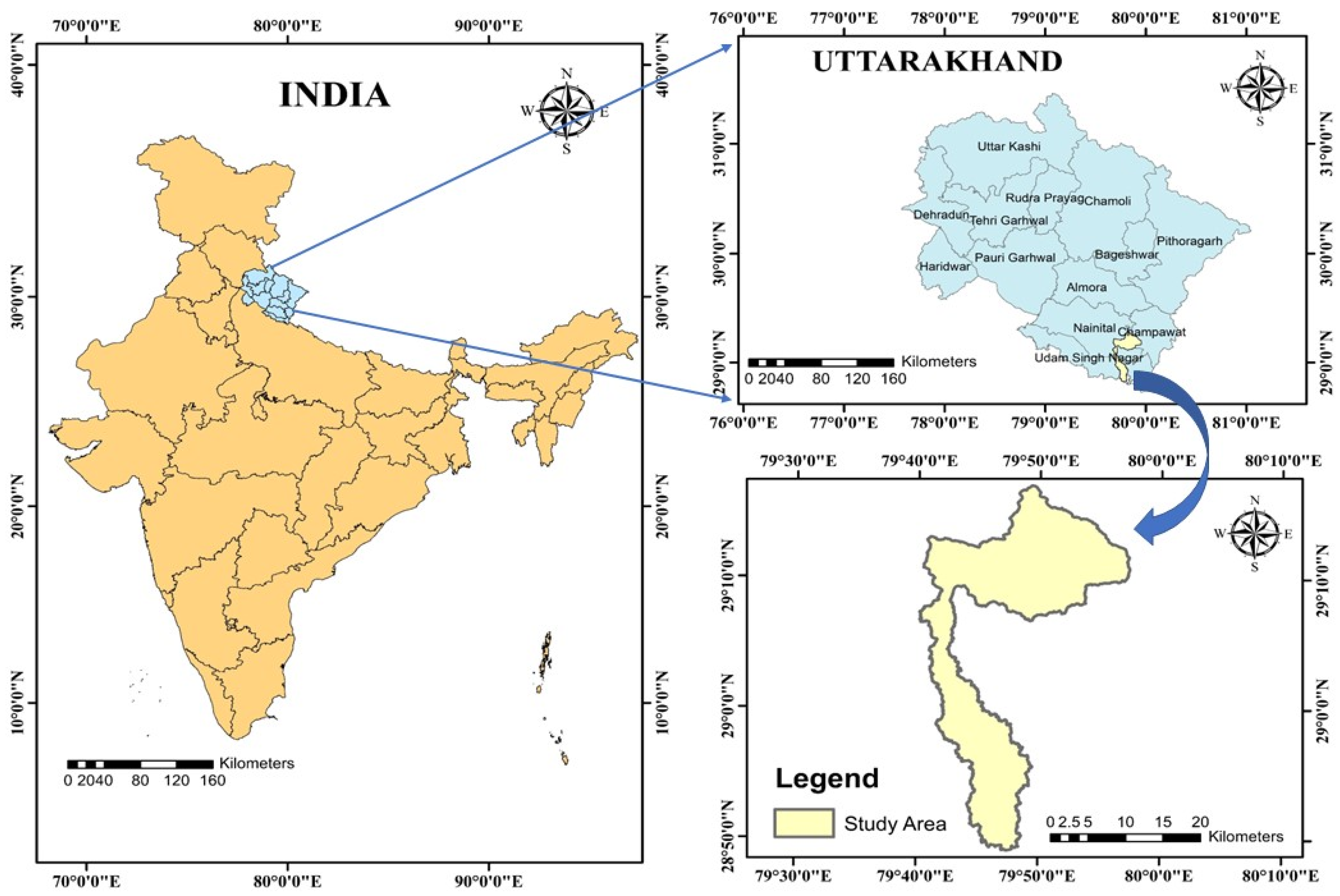
The fact that no previous experiments have been conducted in this watershed for identifying the potential site of groundwater recharge zones is of significant concern since the groundwater table is declining every year. Therefore, it will be beneficial to identify the location of the artificial groundwater recharge zone using rainwater to replenish it. This research aimed to locate the active groundwater recharge zones in Uttarakhand’s Nandhour-Kalish River Watershed. Numerous thematic layers were created by utilizing easily accessible field data, satellite imagery, conventional maps, and the geological, geomorphological, and aquifer characteristics to pinpoint areas of groundwater replenishment. These thematic layers were developed concerning the presence of groundwater. The current methodology provides a reasonable estimation that can benefit a significant portion of the global scientific community.

2. Materials and Methods

2.1. Study Area

The Nandhour-Kailash River watershed, located in the Kumaon region of Uttarakhand, has an area of 474.094 km² and a perimeter of 276.207 km. The location and spread of the Nandhour-Kailash River watershed are shown in Figure 1. It lies in the Tarai and Bhabhar regions of Udham Singh Nagar district and the hilly region of the Nainital and Champawat districts. The Nandhour-Kailash River originates from the Kundal River Forest in the Champawat district. The study area is situated between longitudes and latitudes in the Udham Singh Nagar (78°45′ E–80°08′ E and 28°53′ N–29°23′ N), Nainital (79°27′ E–29°22′ N), and Champawat (80°05′ E–29°20′ N) districts of Uttarakhand. The district comprises seven developmental blocks and seven tehsils, including Japsur, Kashipur, Bazpur, Gadarpur, Rudrapur, Sitargunj, and Khatima, with Rudrapur serving as the district’s administrative center.

The study area has a subtropical to sub-humid climate with three distinct seasons: the summer, the monsoon (rainy season), and the winter. Summertime temperatures reach a high of 42 °C, while wintertime temperatures range from 1 °C to 4 °C. Rainfall intensity increases from south to north, while total precipitation decreases from west to east. The Monsoon season accounts for 90% of rainfall, with the remaining 10% falling outside this time frame. There is an extensive network of drainage systems in the district of Udham Singh Nagar. The average annual rainfall is 40.00 mm (June 2018 to 19 March 2023, with 1713 observations).

2.2. Data Sources and Software Used and Methodology

The Nandhour-Kailash River Watershed study area boundaries were determined using topographic sheets, digital elevation models (DEMs), soil and land use, and land cover (LULC) data sourced from multiple organizations, including the Survey of India (SOI) in Dehradun, Uttarakhand, Alaska Satellite Facility (ASF), National Atlas and Thematic Mapping Organization under the Department of Science and Technology, Government of India, and the United Nations (UN) and Food and Agriculture Organization (FAO). Topographic maps, satellite images, and other reference maps acquired from various sources were used to prepare the LULC characteristics. The data sources used for mapping groundwater potential are shown in Table S1. The study used ArcGIS v10.4.1 to produce and project maps, gather geospatial data, assess mapped data, share and discover geographic data, use maps and geographic data in various applications, and manage geographic data in a database. Figure 2 depicts the methodological flowchart for delineating the Nandhour-Kailash River Watershed. Identifying an appropriate potential zone for artificial groundwater recharge is a wide range of multi-objective and multi-criteria problems. The step-by-step procedure for delineating watersheds and sub-watersheds is shown in Figure 3a.

2.3. Morphometry Analysis

Understanding the morphological features of a catchment area is crucial to understanding the hydrological processes and putting mitigation measures in place [62]. Bali et al. [63] used morphometrics to study the morphology of upper Himalayan zones (now categorized as hydrologic mechanisms). This technique helps understand glacial–fluvial landform development. Linear characteristics for each sub-watershed include stream order, basin length, stream number, average stream length, stream length ratio, and bifurcation ratio. Area characteristics include basin area, perimeter, drainage density, stream frequency, drainage texture, length of overland flow, elongation ratio, circulatory ratio, compactness coefficient, and shape factor. Relief metrics involve maximum and minimum elevation, basin relief, relief ratio, relative relief, ruggedness number, and hypsometric integral. A visual representation of the prioritization methodology for sub-watersheds in the Nandhour-Kailash River Watershed can be found in Figure 3b.

2.3.1. Morphometry Analysis

Linear characteristics include the number, order, and length of streams and their connection.

Stream Order (u)

Horton [64] established a stream ordering approach and quantified the structure of a drainage basin stream system. Horton’s ordering scheme was revised by Strahler [65], and this method was preferred because of its simplicity and lack of subjective views. The streams were arranged in the following order:

• A stream of order (u + 1) is created when two streams of the same order combine;
• The section downstream preserves the higher order of the combining streams when two streams of different orders merge.

Stream Numbers (N_u)

The total number of streams in each order of the watershed is added together to obtain the stream number. N_u denotes the total number of streams in the watershed, counted as stream segments in sequence ‘u’.

Stream Length (L_u)

Each order’s distinct stream segment’s total length is the order stream length. With each stream order, the length of the stream potentially increases [66]. It exposes the features of surface runoff. It can be stated mathematically as:

$$L_u= \sum _{i=1}^{N_u}{L}_i$$

(1)

where N_u = total number of streams of order ’u’; L_u = stream length of order ’u’; and L_i = length of the i^th segment of stream of order ’u’.

Average Stream Length (L_u’)

The average or mean length of a stream is calculated as the ratio of the total length of all streams in a given order (L_u) to the total number of streams in that order (N_u) [66]. Horton’s law of stream length states that direct geometric series with the first term equal to the mean length of the first-order stream can be used to estimate the mean length of streams of various orders in a specific drainage basin. It is a dimensionless property that can be stated mathematically as:

$${L’}_u=\frac{{\sum }_{i=1}^{Nu}{L}_i}{N_u} \mathrm{or} {L’}_u=\frac{L_u}{N_u}$$

(2)

where L’_u = average or mean length of stream of order ‘u’; L_u = length of stream of order ‘u’; L_i = length of the ith segment of stream of order ‘u’; and N_u = total number of streams of order ‘u’.

Stream Length Ratio (R_L)

The stream length ratio is the ratio of the total length of one order of stream segment (u) to the next lower order of stream segment (u − 1) [66]. It can be stated mathematically as:

$$R_L=\frac{{L^{’}}_u}{{L^{’}}_{(u-1)}}$$

(3)

where R_L = stream length ratio; L’_u = average or mean length of stream of order ‘u’; and L’_(u-1) = average or mean length of order ‘u − 1’. The normalized stream-length ratio (R_L), representing the stream-length ratio for the watershed and sub-watersheds, was calculated using Horton’s Law of Stream Lengths [64]. It claimed that the average length of streams (L_u) of each subsequent order tended to resemble a geometric sequence where the term before it represented the average length of first-order streams (L₁) and is expressed as:

$$L_u={L_1\times R}_L^{u-1}$$

(4)

Taking both standard sides, the log in Equation (4) gives:

$$\mathit{log}\left(L_u\right)=(\mathit{log}\left(L_1\right)-\mathit{log}\left(R_L\right))+\mathit{log}\left(R_L\right)\times u$$

(5)

The average length of streams of various orders was used to generate a scatter plot between u and log (L_u), and a linear line of best fit/trendline was fitted to the developed plot.

The trendline (m) slope equals the log (R_L). The R_L was calculated as follows:

$$R_L={10}^m$$

(6)

Bifurcation Ratio (R_b)

Understanding the shape of the basin and the way that runoff behaves is useful. The bifurcation ratio is the proportion of stream segments of a particular order ‘N_u’ to stream segments of the next higher order (N_u + 1). It is a unitless measure that illustrates the degree of integration among streams of different orders within a river basin [66]. R_b values are divided into low (less than five) and high (more than five). Low class indicates that geologic structures do not affect drainage patterns. The bifurcation ratio of successive-order streams may not be uniform due to the drainage basin’s geological and lithological development [47]. The R_b has been computed as:

$$R_b=\frac{N_u}{N_{(u+1)}}$$

(7)

where R_b = bifurcation ratio; N_u = total number of streams of order ‘u’; and N_{(u + 1)} = total number of order ‘u + 1′. The bifurcation ratio for the watershed and sub-watershed, known as the normalized bifurcation ratio (R_b), was determined using Horton’s Law of Stream Numbers [67]. It is written as follows:

$$N_u=R_b^{K-u}$$

(8)

Taking both standard sides, the log in Equation (8) gives:

$$\mathit{log}\left(N_u\right)=K\times \mathit{log}\left(R_b\right)-\mathit{log}\left(R_b\right)\times u$$

(9)

The streams of varying order were used to generate a scatter plot of u vs. log (N_u), and a linear line of best fit/trendline was fitted to create a plot. The trendline slope (m) was equal to the inverse of log (R_b). The R_b was then calculated as follows:

$$R_b={10}^{-m}$$

(10)

Basin Length (L)

It is the separation along the basin’s boundary between the outlet and the furthest point [68]. It is measured in kilometers and may be calculated using the following formula:

$$L=1.3.12\times A^{0.568}$$

(11)

where L = basin length (km); and A = area of the basin in km².

2.3.2. Areal Aspects

Different morphometric parameters characterizing the area have been included in areal aspects as follows.

Basin Perimeter (P)

The outer edge of the sub-basin enclosing the basin’s area is known as the perimeter. The ArcGIS v10.4.1 software calculated the basin’s perimeter.

Basin Area (A)

It is the area enclosed within the watershed boundary divided by the basin area. It is the most essential characteristic of hydrological analysis. More of the higher area will be the runoff from the basin. ArcGIS v10.4.1 was used to calculate the basin’s area.

Drainage Density (D_d)

Drainage density is calculated by dividing the sum of all streams and rivers in a drainage basin by its total area. Strahler [66] used the following equation to express drainage density:

$$D_d=\frac{L_u}{ A}$$

(12)

where D_d = drainage density (km/km²); L_u = length of stream of order ‘u’; and A = basin area in km². Climate, land cover, soil qualities, relief, and landscape evolution processes all influence drainage density in drainage basins [69,70,71]. According to Smith [72], drainage density is categorized into five classes (very coarse (less than 2 km/km²), coarse (2–4 km/km²), moderate (4–6 km/km²), fine (6–8 km/km²), and very fine (more than 8 km/km²)), as shown in Table S2.

Stream Frequency (F_s)

The number of streams per square foot is known as F_s. It can be computed using the drainage density and F_s relationship [64]. F_s is proportional to lithological properties. It can be defined as:

$$\begin{gathered} F_{s }=0.694\times D_{d^2} \\ or \\ {F}_s=\frac{N_u}{A} \end{gathered}$$

(13)

where F_s = stream frequency (km⁻²); D_d = drainage density of the basin (km/km²); N_u = total number of streams of order ‘u’; and A = area of the basin in km².

Drainage Texture (T)

Drainage texture is the sum of all stream segments across all orders within a basin expressed as a unit of basin perimeter [72]. It is a gauge of channel spacing closeness influenced by the environment, including the amount of precipitation, vegetation, lithology, infiltration capacity, and terrain relief [72]. It can be calculated as follows:

$$T=D_d\times F_s$$

(14)

where T = drainage texture (km⁻¹); D_d = drainage density of basin (km/km²); and F_s = stream frequency (km⁻²).

Length of Overland Flow (L_g)

It measures the water’s distance before condensing into a particular stream channel. Drainage density divided by its reciprocal gives the length of an overland flow [64]. This factor is significantly correlated with the length of sheet flow and inversely proportional to the average channel slope and is expressed by the following formula:

$$L_g=\frac{1}{2D_d}$$

(15)

where L_g = length of overland flow (km) and D_d = drainage density of the basin (km/km²). According to Chandrashekar et al. [73], a low L_g value denotes short flow paths, high relief, more runoff, and less infiltration. In contrast, a high value denotes long flow paths, low runoff, high infiltration, and a gentle slope. As shown in Table S3, there are three categories for the length of overland flow, i.e., low (less than 0.2), medium (0.2–0.3), and high (more than 0.3).

Elongation Ratio (R_e)

The ratio of a circle’s diameter to its maximum length has the same area as the drainage basin [74]. The maximum basin length is represented by a value ranging from 0 to 1. It can be defined using the following formula:

$$R_e=\frac{ 1.128\sqrt{A}}{L}$$

(16)

where R_e = elongation ratio of the watershed; A = area of the basin (km²); and L = length of the basin (km). Watersheds are divided into numerous types based on their elongation ratio [65], as shown in Table S4. In general, the larger the watershed, the higher the peak runoff at the outlet, and vice-versa. Elongation ratios of 0.6 to 0.8 are frequently associated with high relief and steep ground slopes. Locations with very little relief, on the other hand, typically have values that are close to 1.0 [65]. Compared to an elongated basin, a circular basin has higher discharge runoff efficiency [75].

Circulatory Ratio (R_c)

The circulatory ratio is the ratio of the basin’s size to the surface area of a circle with the same perimeter as the basin [76]. Instead of the basin slope and drainage pattern, the circularity ratio, which ranges from 0 to 1, is affected by the frequency, length, land use/land cover of streams, geological features, relief, and climate [66]. The circulatory ratio can be expressed mathematically as:

$$R_c= 4\pi \left(\frac{A}{P^2}\right)$$

(17)

where R_c = circulatory ratio of the watershed; A = area of the basin (km²); and P = perimeter of the basin (km).

Form Factor (F_f)

The form factor is a quantitative measure of drainage basin outline. It is described as the relationship between basin area and basin length squared. It shows the amount of water flowing through a basin in a specific area [67]. The form factor may be calculated using the following formula:

$$F_f=\frac{A}{L^2}$$

(18)

where F_f = form factor of the watershed; A = area of the basin (km²); and L = length of the basin (km). The basin will be longer if F_f is smaller. Low-form factor elongated drainage basins have lower peak flows that last longer. However, basins with increased form factors experience short-lived, high-peak flows [64].

Compactness Coefficient (C_c)

It is the ratio of the watershed’s perimeter to the circumference of a circle whose area is equal to its perimeter [77]. It is employed to demonstrate the relationship between a circular basin of similar area and a hydrological basin, as shown below:

$$C_c=0.282 \frac{P}{A^{0.5}}$$

(19)

where C_c = compactness coefficient of the watershed; P = perimeter of the basin (km); and A = area of the basin (km²). C_c values greater than one indicate less elongation and more erosion. In contrast, values less than one indicate more elongation and less erosion. The basin is circular if the compactness coefficient is 1 [64].

Shape Factor (S_f)

The shape and form factors are inversely proportional [67]. It is described mathematically as the proportion of the basin area to the square of the basin length, and it is written as:

$$S_f=\frac{L^2}{A}$$

(20)

where S_f = shape factor of the watershed; L = length of the basin (Km); and A = basin area (km²).

2.3.3. Relief Aspects

The watershed landforms’ area, volume, and altitude indicate a drainage basin’s relief [74].

Basin Relief

It is defined as the difference in elevation between the basin’s maximum and minimum elevations, impacting channel spacing and sediment movement [65]. It can be calculated using the following relationship:

$$Basin relief=H-h$$

(21)

where H = maximum elevation in the basin (km) and h = minimum elevation in the basin (km).

Relative Relief (R_r)

Relative relief aims to determine the amplitude of available relief related to the altitude of a given area’s highest and lowest points [78]. It denotes the difference between a spatial unit’s highest and lowest points. It is critical to comprehend the watershed’s denudational characteristics, degree of dissection, and terrain’s morphological characteristics. These parameters control the stream gradient and, thus, influence the flood pattern [79]. It can be expressed as:

$$R_r=\frac{H-h}{P} \times 100$$

(22)

where R_r = relative relief of the watershed; P = perimeter of the basin (km); H = maximum elevation in the basin (km); and h = minimum elevation in the basin (km).

Relief Ratio

The relief ratio represents the longest dimension aligned with the primary drainage route. It is a dimensionless ratio of height to length, defined as the tangent of the angle between two planes meeting at the basin’s outlet: one plane represents the horizontal, while the other passes through the highest point in the basin. The relief ratio provides insight into the overall slope of a drainage basin. It displays the erosion rate on the basin slope in terms of intensity [74]. It can be computed as:

$$Relief ratio=\frac{H-h}{L}$$

(23)

where L = length of the basin (km); H = maximum elevation in the basin (km); and h = minimum elevation in the basin (km).

Ruggedness Number (R_n)

It is the result of drainage density and basin relief. The ruggedness number represents the terrain’s structural complexity. When drainage density and relief are both high, and the slope is short but steep, a ruggedness number with a highly high-value result [80]. It can be described mathematically as:

$$R_n=(H-h)\times D_d$$

(24)

where R_n = ruggedness a number of the watershed and D_d = drainage density of the basin (km⁻¹).

Hypsometric Integral (HI)

It is an essential topographical index that represents the watershed growth stage. HI also provides information about the activity strength in the watershed’s geologic features. According to the value of their hypsometric integral (HI), Strahler [80] divided the watershed development stage into three types (HI ≥ 0.60 = youthful or in-equilibrium stage; 0.60 to 0.35 = equilibrium or mature stage, and 0.35 < monadnock or old stage (Table S5)) and is expressed mathematically as:

$$HI=\frac{Mean elevation-Minimum elevation}{Maximum elevation-Minimum elevation}$$

(25)

2.4. Prioritization of Sub-Watersheds Based on Morphometric Analysis

Utilizing RS and GIS techniques, sub-watersheds were prioritized. Sub-watersheds were prioritized using the compound priority (C_P) model [81]. The sub-watershed prioritization was based on several parameters, including bifurcation ratio, stream length ratio, drainage density, drainage texture, length of overland flow, and stream frequency. Those sub-watersheds with the highest values in these parameters received the highest priority. The sub-watershed with the lowest parameter value was granted the highest priority among the remaining parameters, like elongation ratio, circulatory ratio, form factor, compactness ratio, and shape factor. A compound priority value (C_P) was calculated to determine the overall priority. Sub-watersheds were then categorized into three priority classes: high, medium, and low, based on their C_P values [68]. The C_P can be computed as outlined below:

$$C_P=\frac{1}{n}\sum _{i=1}^n{R}_i$$

(26)

where C_P = compound priority, R = rank, and n = number of parameters.

2.5. Delineation of Groundwater Potential Zones

Identification of potential locations for artificial groundwater recharge using the geo-visualization concept. The sites were shown using ArcGIS v10.4.1 software according to the priority set for location identification. The software depicted the watershed region by overlaying the drainage, slope, soil, and land use/land cover maps to locate recharge sites. The requirement and guideline [82] criteria for proposed locations for the water conservation structures are given in Table S6. Using these criteria as guidance, viable locations for farm ponds and check dams were recognized, and suitable farm ponds and check dam sites were suggested.

3. Results

Thematic layers of the controlling factors were applied to identify artificial groundwater potential recharge zones in the study area. Thus, the analysis results in morphometric parameters for the Nandhour-Kailash River watershed utilizing GIS methodologies and prioritizing its sub-watersheds based on the compound priority value (C_p) method used. Also investigated were the suggested locations for artificial groundwater recharge. The following sections provide the study’s findings.

3.1. Digital Elevation Model Processing

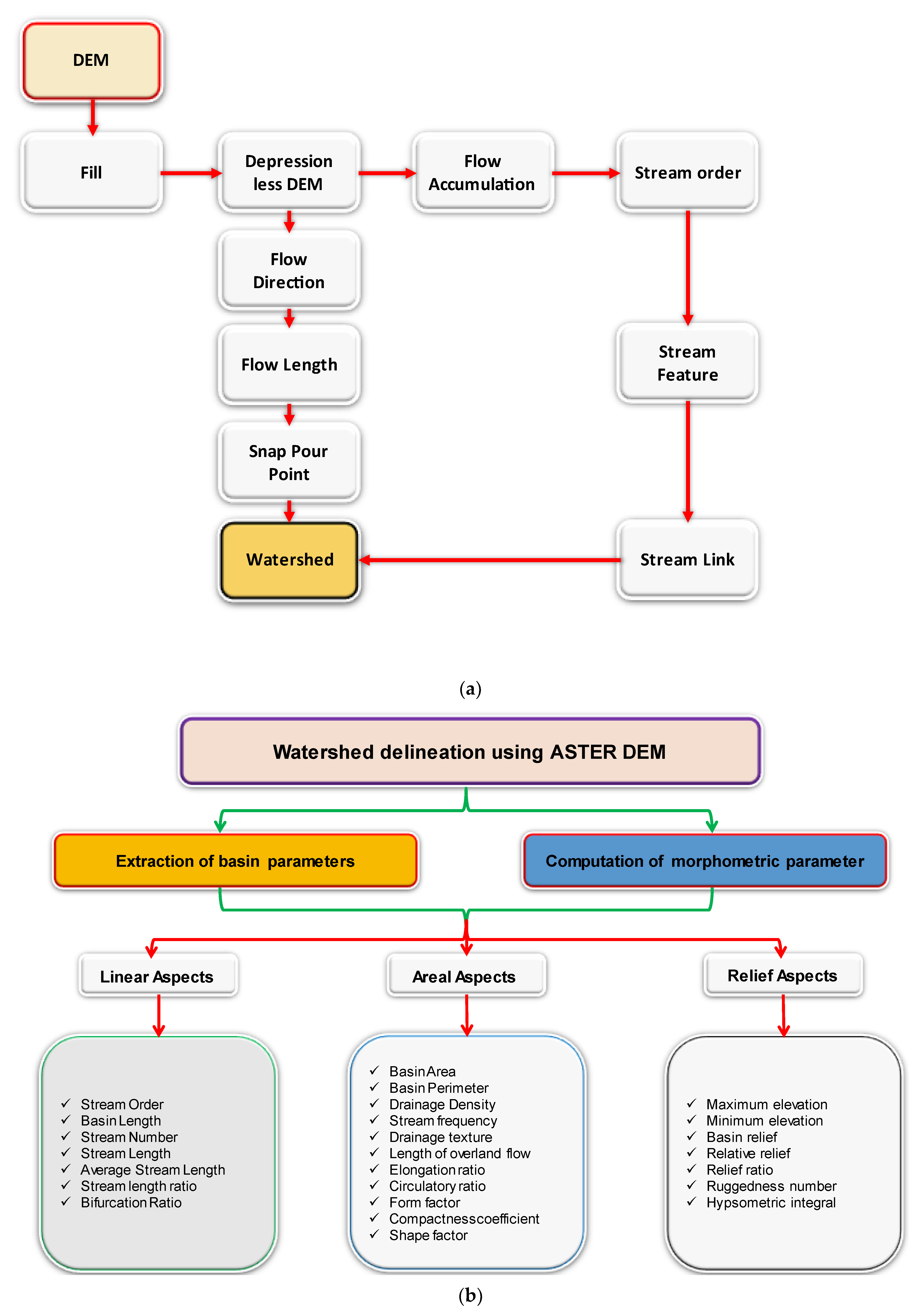
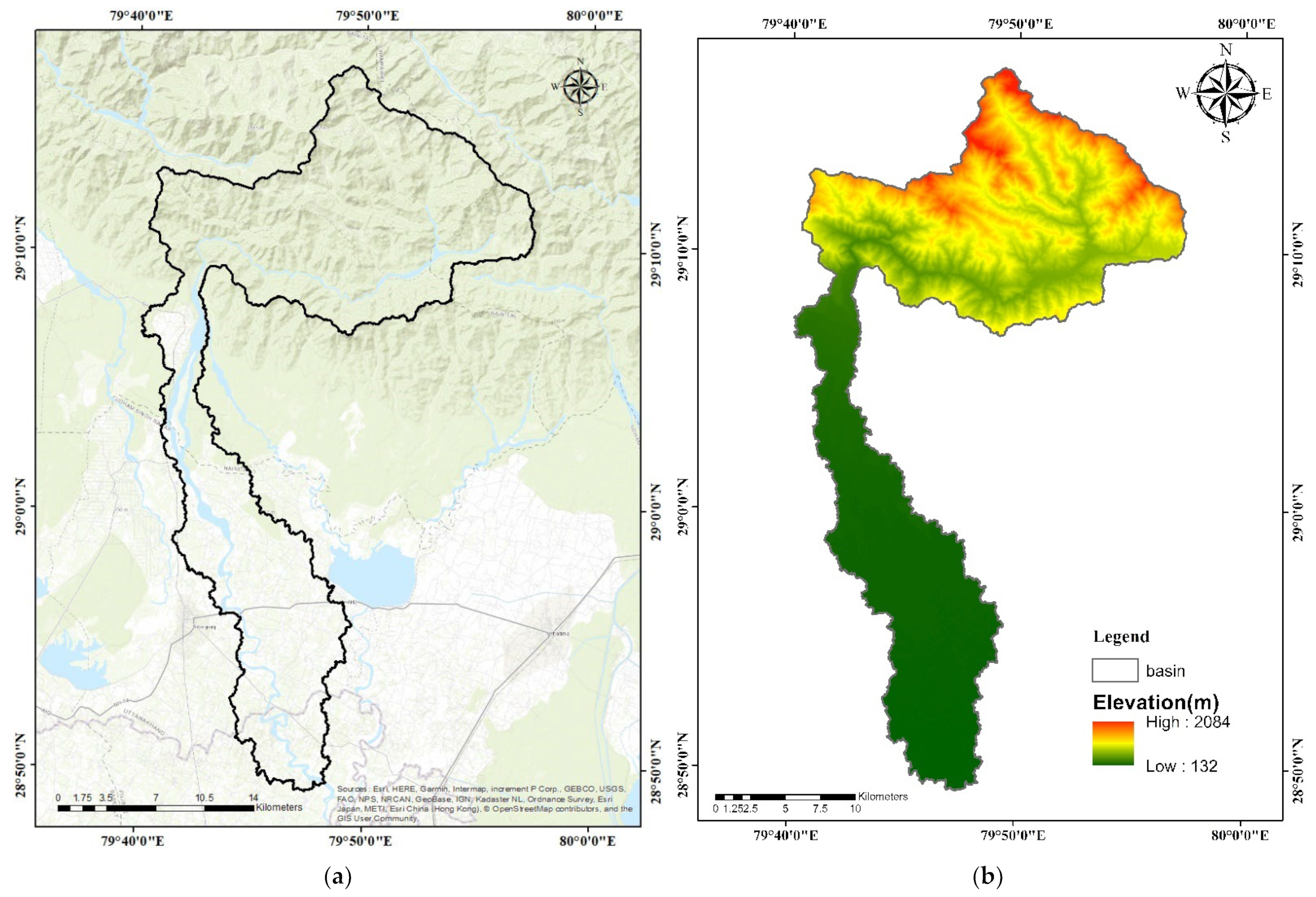
ASTER DEM data retrieved from the ASF website and analyzed with ArcGIS v 10.4.1 software were used to estimate the watershed area. The geographical area of the delineated watershed and perimeter were measured to be 474.094 km² and 276.207 km, respectively. The satellite image of the watershed taken from the USGS Earth Explorer website with a resolution of 30 m × 30 m is shown in Figure 4a. The DEM of the watershed was created using ASTER DEM data retrieved from the ASF website. The elevation of the watershed ranged from 132 m in the valley to 2084 m on the ridges, as shown in Figure 4b. SOI toposheets with a scale of 1:50,000 and satellite data were used to create a base map and drainage network map, among others. The base map was created using SOI toposheets No. 53O11, 53O12, 53O15, 53O16, 53P9, and 53P13 on a scale of 1:50,000. 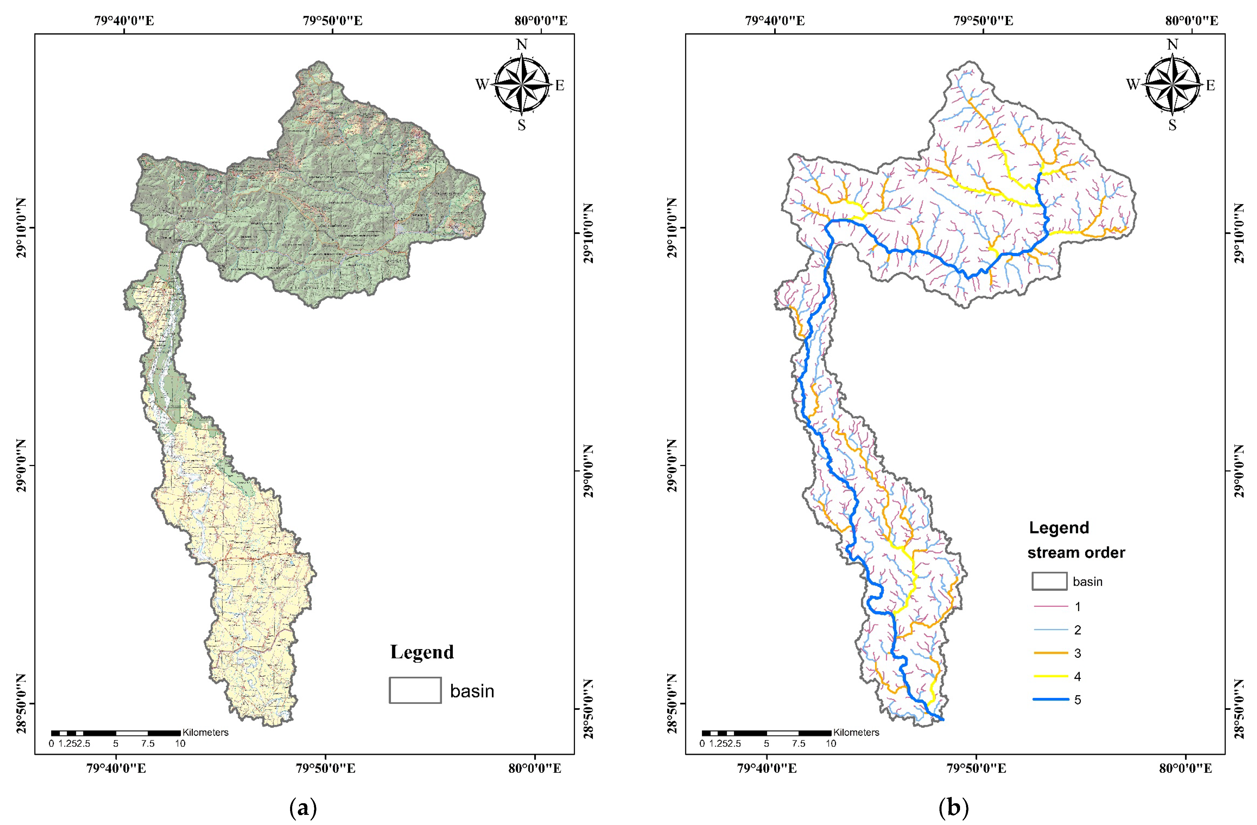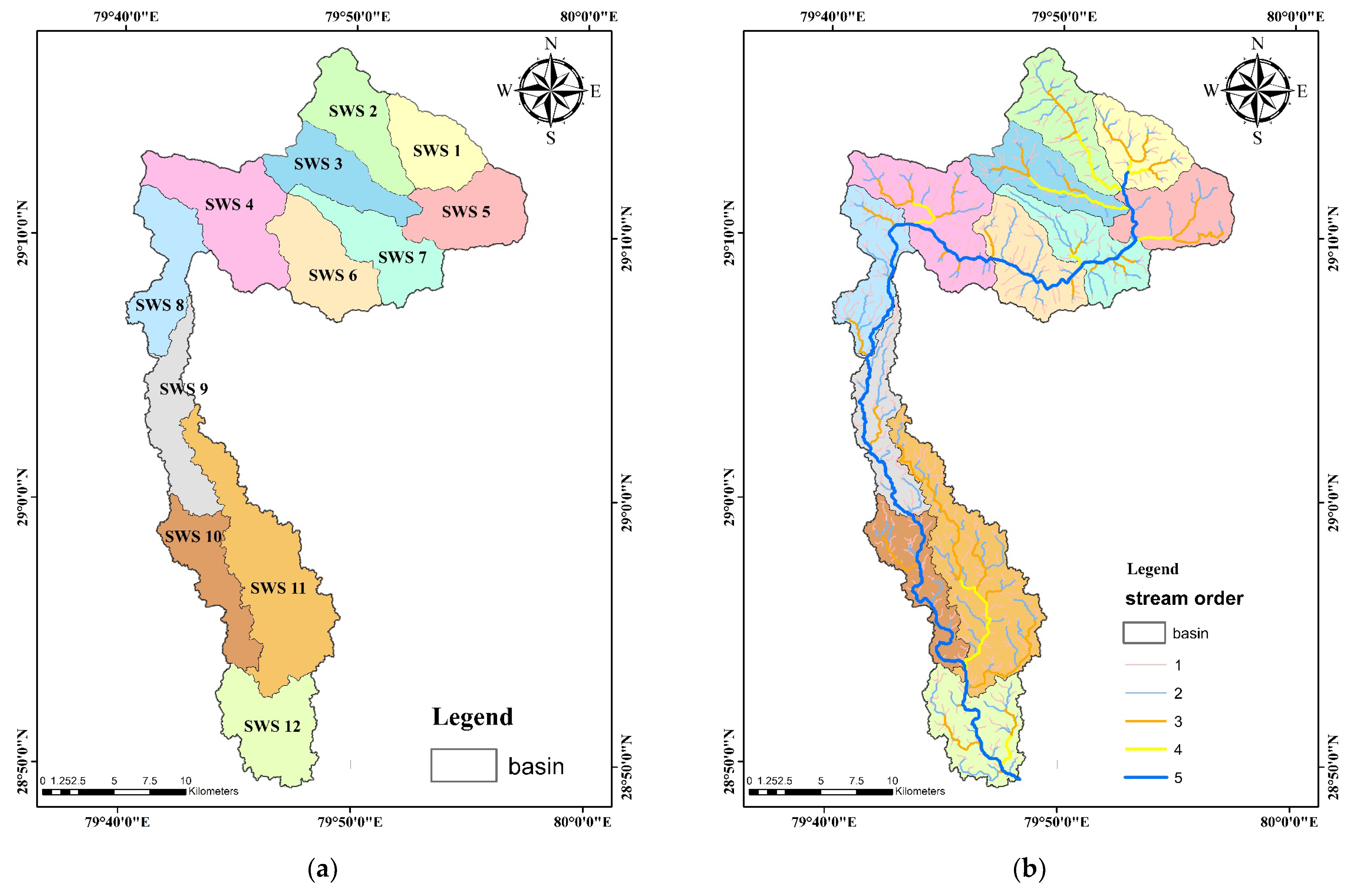The completed map depicts the basic features of the study area, such as forests, agricultural land, and establishments Figure 5a. The drainage network map for the study area was created with the DEM raster file, the flow direction, and the flow accumulation layer from the Hydrology portion of the Arc Toolbox in ArcGIS v 10.4.1 Software “Spatial Analyst Tool” coupled with SWAT 2012. According to the drainage network map, the Nandhour-Kailash River watershed was of the fifth order and had a dendritic drainage network pattern. The Nandhour-Kailash River watershed drainage network map is shown in Figure 5b.

3.2. Morphometric Analysis

The entire watershed area was divided into 12 sub-watersheds (SWS1 to SWS12). It was suitably marked based on drainage patterns and basin area. The area, perimeter, and basin length of the watershed and its sub-watersheds are shown in Table S7. The sub-watershed area was 29.092 km² for SWS1 and 76.062 km² for SWS11. The maximum perimeter was found to be 99.77 km of the SWS11 sub-watershed. Its minimum value was compared with the SWS1 sub-watershed (31.05 km). The delineation of the sub-watersheds and the drainage network of each sub-watershed are depicted in Figure 6a and Figure 6b, respectively.

3.2.1. Linear Aspects

The Nandhour-Kailash River watershed’s linear parameters, such as stream order, stream length, bifurcation ratio, basin length, etc., were calculated. The drainage network in the study area was used to estimate different linear characteristics. Table S8 shows several linear characteristics and their relationships, as proposed by other scientists.

The watershed of the Nandhour-Kailash River was of the fifth order. However, out of 12 sub-watersheds, 10 sub-watersheds (SWS1, SWS4, SWS5, SWS6, SWS7, SWS8, SWS9, SWS10, SWS11, and SWS12) were of the fifth order, and two sub-watersheds (SWS2, SWS3) were of the fourth order. As shown in Table S8, it was found that as stream order increases, the number of streams decreases. In the Nandhour-Kailash River watershed, the first, second, third, fourth, and fifth-order stream numbers were 828, 361, 205, 86, and 1, respectively. First-order streams were highest in sub-watershed SWS11 (N_u = 142) and lowest in sub-watershed SWS1 (N_u = 47). The number of streams for other orders in each sub-watershed is shown in Table S9. The first-order streams were 413.904 km long, 193.019 km long, 107.496 km long, 37.855 km long, and 80.785 km long, respectively. The maximum stream length (L_u = 74.729 km) was found in sub-watershed SWS11, while the smallest stream length (L_u = 22.055 km) was found in sub-watershed SWS1. The stream length in different sub-watersheds is shown in Table S9. The value of L_u’ was 16.556 km, and the values of L_u’ for different orders are presented in Table S8 for the Nandhour-Kailash River watershed and Table S9 for its sub-watersheds. The basin length of the Nandhour-Kailash River watershed was calculated to be 43.43 km, and Table S7 shows the estimated basin length for the 12 sub-watersheds. The normalized stream length ratio for the Nandhour-Kailash River watershed was 0.612 (Table S8). At the same time, normalized values of the stream length ratio for individual sub-watersheds are illustrated in Table S10. It has been found that the likelihood of recharge increases with the stream length ratio. Scatter plots for computation of the normalized stream length ratio in the Nandhour-Kailash River watershed and its sub-watersheds (SWS1 to SWS12) are available in Supplementary Material Figures S1 and S2, respectively. The normalized bifurcation ratio for the Nandhour-Kailash River watershed was 4.424 (Table S8). However, their normalized values observed for individual sub-watersheds are illustrated in Table S10. It was found that the drainage pattern was unaffected by the geologic structures. Scatter plots for the computation of the normalized bifurcation ratio in the Nandhour-Kailash River watershed and different sub-watersheds (SWS1 to SWS12) are shown in Supplementary Material Figures S3 and S4, respectively.

3.2.2. Areal Aspects

The runoff of a drainage basin will be higher as its surface area increases. The watershed area and perimeter of the Nandhour-Kailash River were calculated as 474.094 Km² and 276.207 Km, respectively. Table S7 lists the area and perimeters of each sub-watershed. The drainage density for the Nandhour-Kailash River watershed was calculated to be 1.757 km/km² (Table S11), which indicates a very coarse drainage texture. Table S12 displays the drainage density for each sub-watershed, which corresponds to a very coarse to coarse drainage texture. The Nandhour-Kailash River watershed stream frequency was calculated as 3.123 (Table S11). Table S12 lists the sub-watershed stream frequency. According to Table S11, the study area’s drainage texture, which is 5.489 Km⁻¹, is moderate. Table S12 displays the drainage texture value for sub-watersheds, classified as having a moderate to fine drainage texture. For the Nandhour-Kailash River watershed, the length of overland flow was calculated to be 0.878 (Table S11), representing the high length of overland flow. The value of the length of overland flow for each sub-watershed is shown in Table S12, which represents the medium to high length of overland flow, i.e., long flow paths, low runoff, high infiltration, and gentle slope. The elongation ratio for the Nandhour-Kailash River watershed has been calculated to be 0.565 (Table S11), indicating that the watershed has an elongated shape. The elongation ratios for all sub-watersheds are given in Table S12, indicating that the sub-watersheds have long shapes, i.e., high relief and steep ground slopes. The study area circulation ratio was 0.078 (Table S11). Table S13 displays the circulatory ratio for each sub-watershed. The elongated shape has lower peak flows and longer duration. The form factor for the entire study area was 0.251 (Table S11), indicating a lower flow peak. Table S13 displays the form factor value for each sub-watershed.

The overall compactness coefficient was 3.578 (Table S11), indicating less elongation with increased erosion. Its value for each sub-watershed is shown in Table S13, representing less elongation with increased erosion. The value of the shape factor for the entire study area was 3.97 (Table S11), and Table S13 displays its value for each sub-watershed.

3.2.3. Relief Aspects

The difference in elevation between the reference points located in the basin perimeter before the outlet and the highest point on the basin perimeter following the drainage basin’s discharge is known as the basin relief in the context of a drainage basin. The total basin relief was found to be 1.951 km (Table S14), and for all sub-watersheds, its values are presented in

Table 1. Relief aspects of sub-watersheds of Nandhour-Kailash River watershed.

Sub Watersheds	Perimeter	Max Elevation	Min Elevation	Basin Relief	Relative Relief	Drainage Density	Ruggedness Number	Basin Length	Relief Ratio
SWS1	31.05	1.847	0.627	1.220	3.929	1.511	1.843	8.899	0.137
SWS2	41.45	2.084	0.623	1.461	3.524	1.445	2.112	10.171	0.143
SWS3	42.52	1.930	0.610	1.320	3.104	1.598	2.110	9.258	0.142
SWS4	52.85	1.845	0.367	1.478	2.796	1.592	2.354	12.715	0.116
SWS5	37.57	1.800	0.581	1.219	3.244	1.659	2.022	9.999	0.121
SWS6	38.95	1.724	0.467	1.257	3.227	1.574	1.978	10.408	0.120
SWS7	45.20	1.702	0.537	1.165	2.577	1.628	1.896	9.585	0.121
SWS8	52.17	1.398	0.255	1.143	2.190	1.894	2.165	9.860	0.115
SWS9	65.52	0.277	0.156	0.121	0.184	2.139	0.258	9.504	0.012
SWS10	60.75	0.179	0.141	0.038	0.062	1.999	0.075	9.447	0.004
SWS11	99.77	0.202	0.140	0.062	0.062	2.049	0.127	15.361	0.004
SWS12	52.121	0.159	0.132	0.052	0.051	1.833	0.049	10.725	0.002

. Among the sub-watersheds, the relief of the basins ranged from the lowest (0.038 km) in SW10 to the highest (1.461 km) in SW2. The ratio of basin relief to basin perimeter is called relative relief. The Nandhour-Kailash River watershed had a relative relief value of 0.706 (Table S14). Its value for each sub-watershed is given in Table 1.

Among the sub-watersheds, the relative relief value of the basins ranged from the lowest (0.051) in SW12 to the highest (3.929 km) in SW1. The distance horizontally along the basin’s most extended dimension parallel to the main drainage line divided by the maximum relief is known as the relief ratio. The relief ratio for the Nandhour-Kailash River watershed was 0.044 (Table S14). The value of each sub-watershed is presented in Table 1. Among the sub-watersheds, the relative relief value of the basins ranged from the lowest (0.002) in SW12 to the highest (1.143) in SW2. The relief ratio measures a drainage basin’s overall steepness. It shows how intense the erosion process is on the slope of the basin [74]. The product of drainage density and basin relief yields the ruggedness number. The overall roughness of the watershed was calculated to be 3.428 (Table S14), and all sub-watersheds are given in Table 1. Among the sub-watersheds, the relative relief value of the basins ranged from the lowest (0.049) in SW12 to the highest (2.354) in SW4. 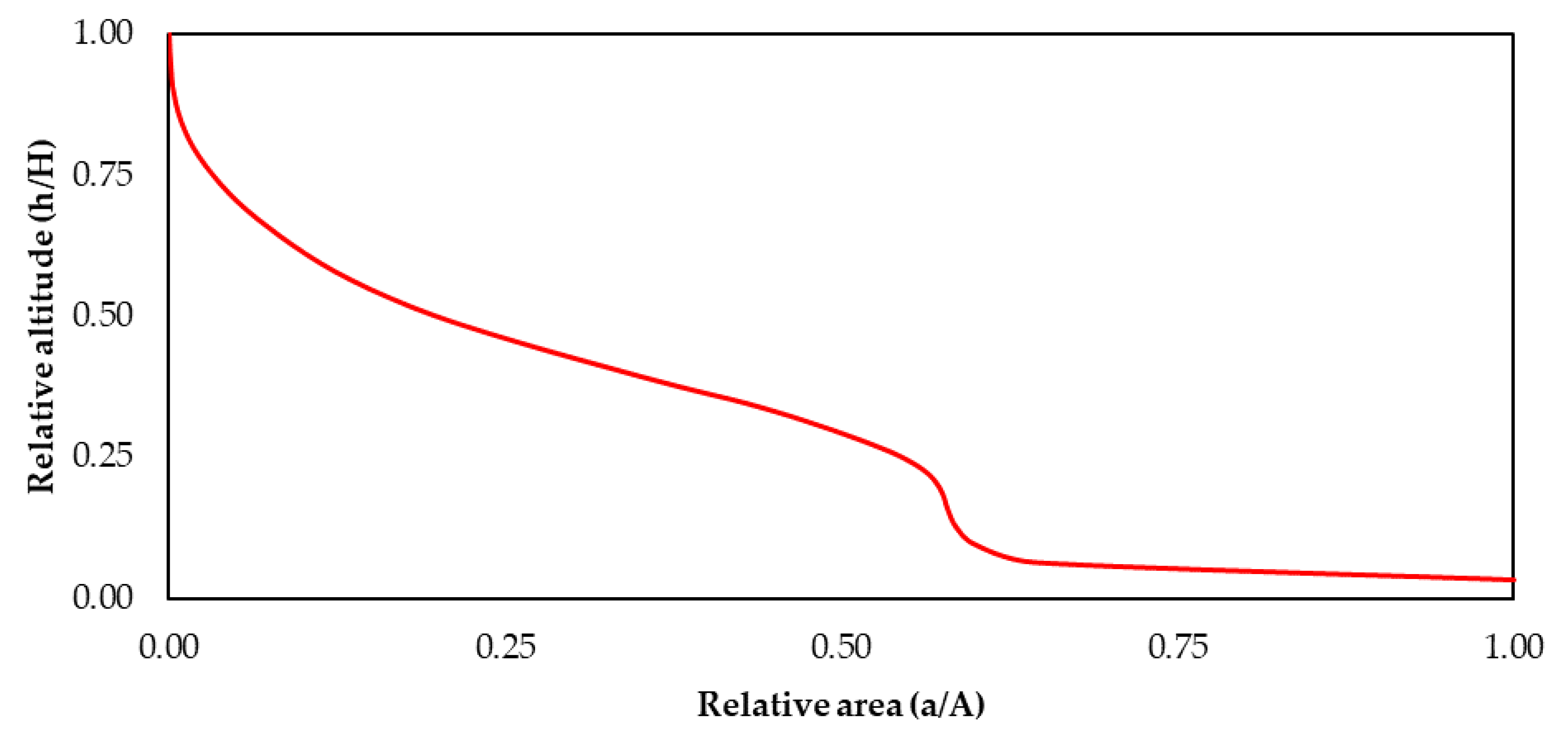The hypsometric integral (HI) is calculated to determine the developmental stage of the study area and to fully understand the strength and level of activity in the watershed’s geologic structure. The estimated HI value was 0.481, as shown in Table S14, indicating that the watershed was in equilibrium or matured. The hypsometric curve for the Nandhour-Kailash River watershed is shown in Figure 7.

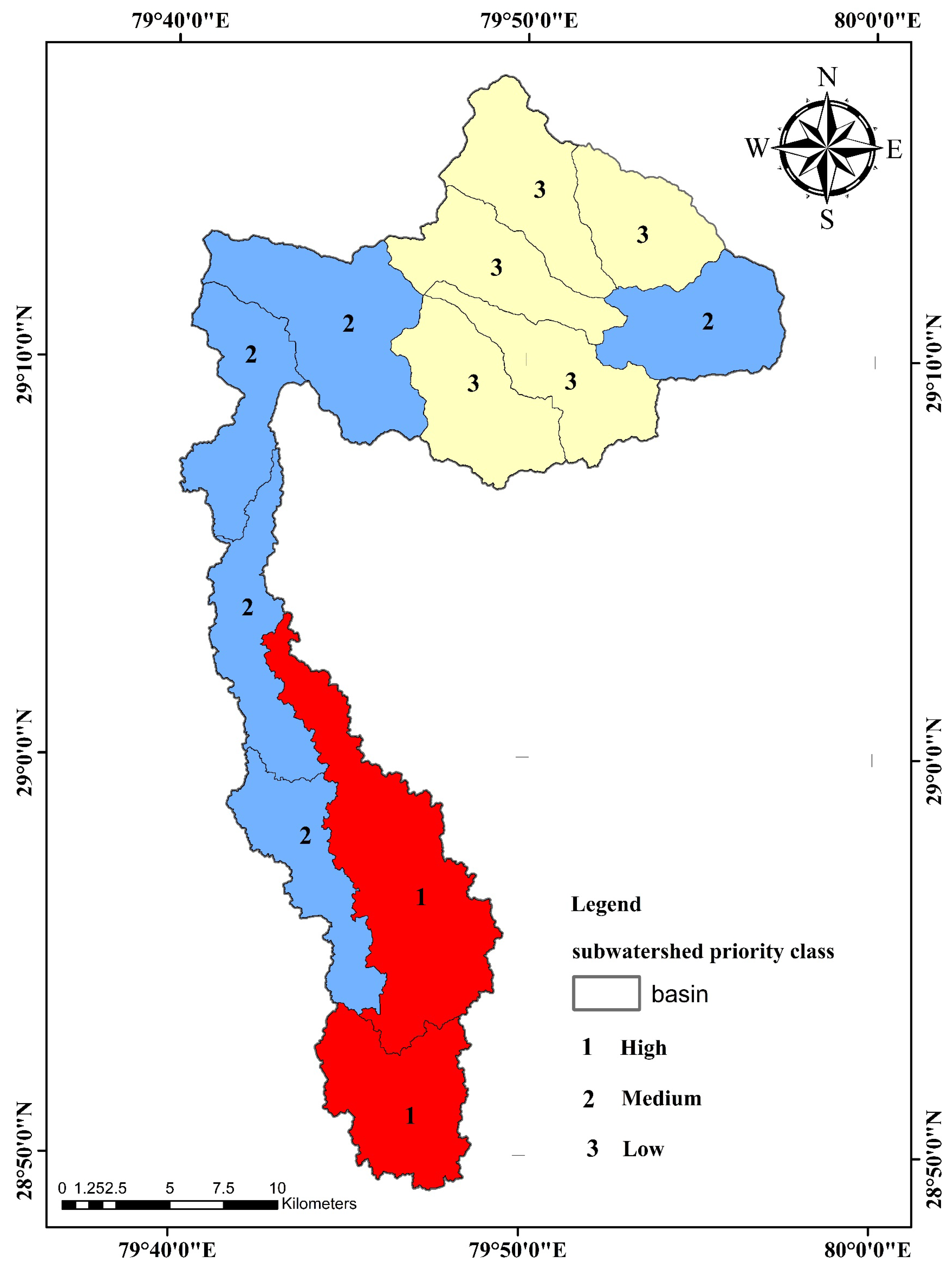
3.3. Sub-Watershed Prioritization Using Morphometric Criteria

As a result of the research, we emphasize the importance of prioritizing the sub-watersheds based on the analysis of morphometric data.

Table 2. Sub-watershed priority rankings based on morphometric criteria.

Sub-Watersheds	Morphometric Criteria											CP	Final Priority
	RL	Rb	Dd	Fs	T	Lg	Re	Rc	Ff	Cc	Sf
SWS1	9	11	11	3	9	2	12	12	12	1	1	7.545	12
SWS2	10	12	12	4	10	1	5	9	5	4	8	7.272	10
SWS3	8	1	8	7	8	5	11	7	11	6	2	6.727	8
SWS4	4	5	9	11	11	4	2	8	2	5	11	6.545	7
SWS5	5	10	6	5	6	7	6	11	6	2	7	6.454	5
SWS6	6	7	10	12	12	3	4	10	4	3	9	7.272	10
SWS7	11	8	7	6	7	6	8	6	8	7	5	7.181	9
SWS8	1	9	4	10	5	9	7	4	7	9	6	6.454	5
SWS9	2	6	1	9	2	12	9	1	9	12	4	6.090	4
SWS10	3	3	3	8	3	10	10	3	10	10	3	6.000	3
SWS11	12	2	2	1	1	11	1	2	1	11	12	5.090	1
SWS12	7	4	5	2	4	8	3	5	3	8	10	5.363	2

and

Table 3. Categorization of sub-watersheds.

Ranking Range (CP Value)	Priority Value	Priority Class	Sub-Watersheds	Area (km2)
<5.908	1	High	SWS 11, SWS 12	116.470
5.908–6.727	2	Medium	SWS 4, 5, 8, 9, 10	190.129
>6.727	3	Low	SWS 1, 2, 3, 6, 7	168.584

show the overall score and the sub-watersheds priority rankings and their classification into various priority classes based on C_p values. The sub-watersheds’ highest and lowest prioritized scores were 7.545 and 5.090, respectively. The Cp’s lower (higher) value indicates a high (low) priority class.

High-priority sub-watersheds show more significant soil erosion and may be a good location for creating and managing soil conservation strategies. The sub-watersheds SWS11 and SWS12 were classified as high-priority sub-watersheds, which covered an area of 116.47 km² (Table 2), and immediate attention for soil and water conservation is required. The sub-watersheds SWS4, SWS5, SWS8, SWS9, and SWS10, with a total area of 190.129 km², were found to be a medium priority and have moderate soil erosion and land degradation. The SWS1, SWS2, SWS3, SWS6, and SWS7 sub-watersheds, with an area of 168.584 km², were found to be low priority and are at low risk of soil erosion and degradation (Table 2). Then, using ArcGIS, a final C_P prioritized map of Pindar’s sub-watersheds was produced with priority rankings (Figure 8).

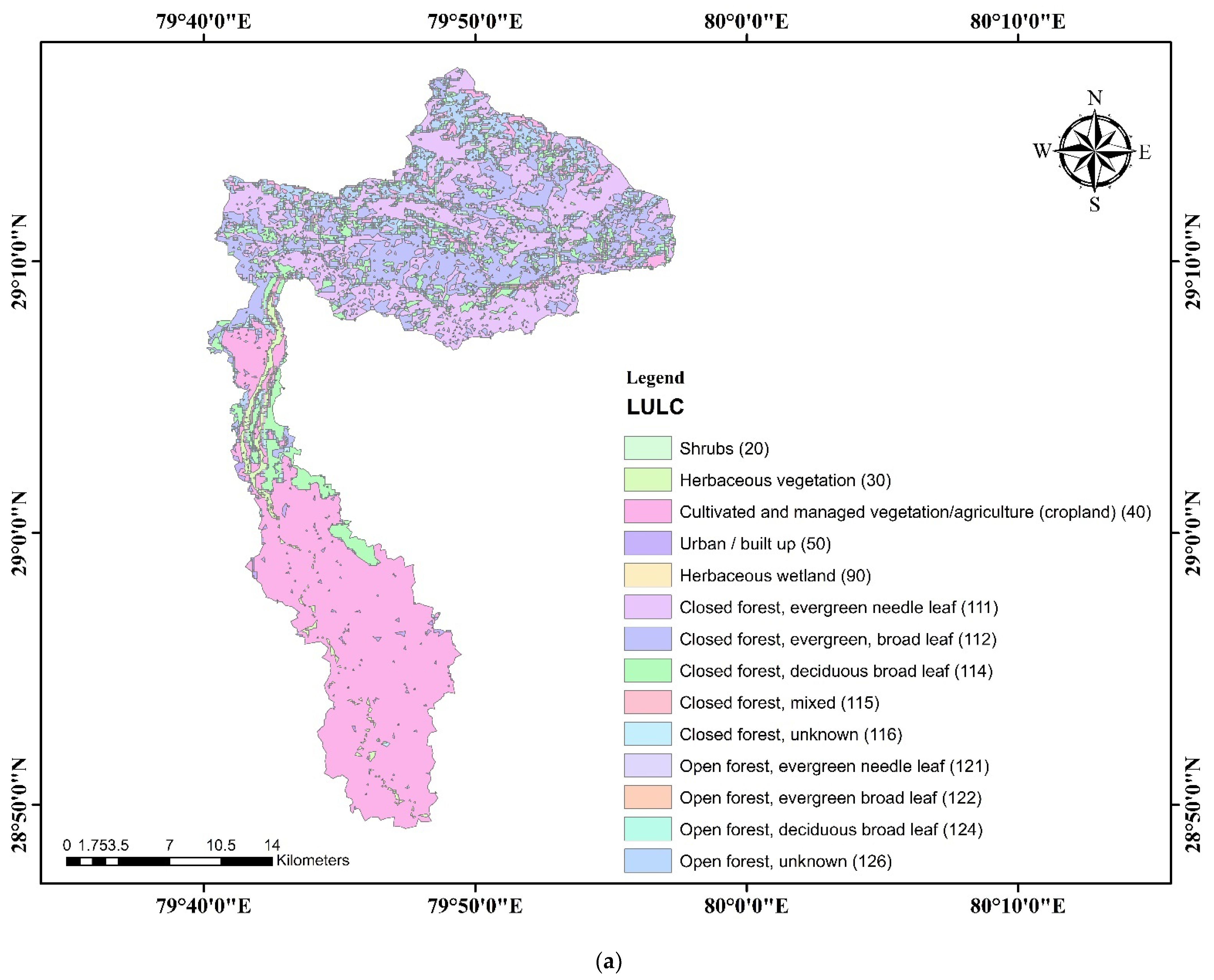
3.4. Land Use and Land Cover (LULC)

Identifying the current LULC pattern and its effects on water resources is fundamental in watershed planning. The LULC map of the Nandhour-Kailash River watershed is shown in Figure 9a. The classification of LULC revealed that the study area was covered with shrubs, herbaceous vegetation, cultivated and managed vegetation/agriculture (cropland), urban/built up, herbaceous wetland, closed forest (evergreen needle leaf, evergreen, broad leaf, broad, deciduous leaf, mixed, unknown), and open forest (evergreen needle leaf, broad evergreen leaf, vast, deciduous leaf, unknown) with corresponding areas of 1.54 km², 7.91 km², 171.62 km², 3.09 km², 0.11 km², 252.77 km², and 36.84 km², while the LULC classification revealed that maximum area (171.62 km²) was covered by cultivated and managed vegetation/agriculture (cropland). Open forests and broad evergreen leaves covered the minimum area (0.43 km²).

Table 4. Land use/land cover classification in the Nandhour-Kailash River watershed.

Map Code	Land Use Class	Area (km2)	Total Area (km2)
20	Shrubs	1.54	1.54
30	Herbaceous vegetation	7.91	7.91
40	Cultivated and managed vegetation/agriculture (cropland)	171.62	171.62
50	Urban/built-up	3.09	3.09
90	Herbaceous wetland	0.11	0.11
111	Closed forest, evergreen needle leaf	120.15	252.77
112	Closed forest, evergreen, broad leaf	76.81
114	Closed forest, broad, deciduous leaf	43.36
115	Closed forest, mixed	0.10
116	Closed forest, unknown	12.35
121	Open forest, evergreen needle leaf	1.19	36.84
122	Open forest, evergreen broad-leaf	0.43
124	Open forest, broad, deciduous leaf	1.98
126	Open forest, unknown	33.24

displays the area that each class of LULC covers.

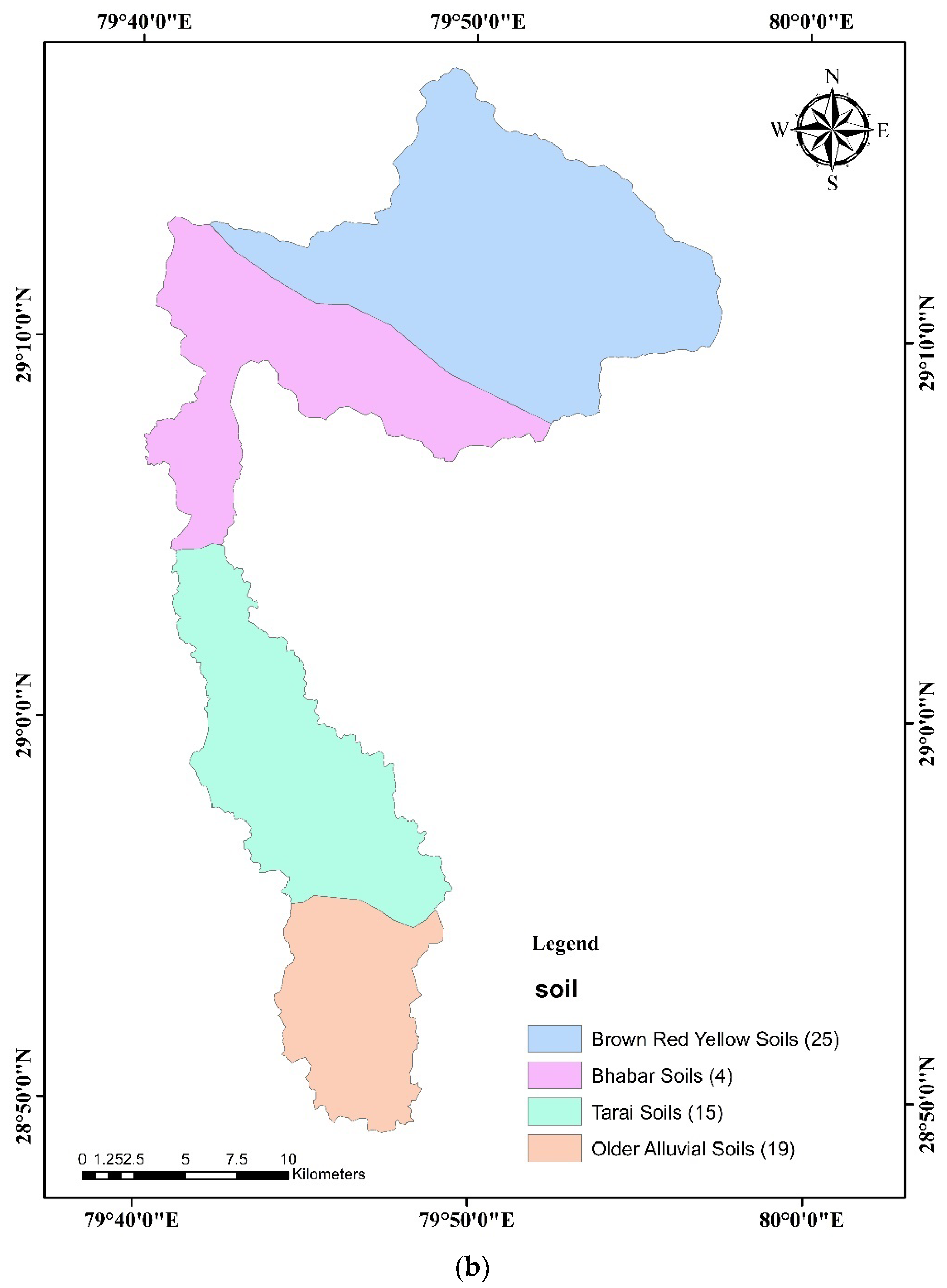
3.5. Soil Classification

Soil is an essential factor that determines potential groundwater zones. A region’s infiltration rate and water-holding capacity are heavily influenced by soil type and permeability [83]. The image was geo-referenced, projected to the exact coordinates as the base map, and saved as a raster file. In addition, a shape file for the soil map of the study area was also created. The study area base map was superimposed on the Northern India raster soil map. The ArcGIS editor tool was used to create the soil map of the study area. According to the analysis of the soil types, the study area was covered in brown and red soil. Yellow soil, Bhabar soil, Tarai soil, and older alluvial soil had areas of 192.52 km², 108.25 km², 109.86 km², and 63.88 km², respectively (Figure 9b), and information about texture, area, and suitability of crops for various soil classes is given in

Table 5. Classification of soil in the Nandhour-Kailash River watershed.

Map Code	Name of Soil	Texture	Area (km2)	Suitability for Crops
3661	Brown red yellow soil	Silty clay loam	192.52	Groundnut, Pulses, Millet, Cotton, Tobacco
3661	Bhabar soil	Clay loamy	108.25	Wheat, Sugarcane, Cotton, Jute, Pulses, Oilseeds, Vegetables
3851	Tarai soil	Sandy loam	109.86	Wheat, Rice, Sugarcane, Jute
3851	Older alluvial soil	Sandy clay	63.88	Sugarcane, Rice, Cotton, Maize, Wheat, Tobacco, Jute, Oilseeds

.

3.6. Terrain Analysis

Using geographic information systems, terrain analysis examines topographic features. These characteristics include slope, aspect, hill shade, elevation, contour lines, flow direction, and upslope and downslope flowlines. It links ecological processes with physical characteristics. The study area’s hillside, contour, slope, and aspect were mapped using the ArcGIS v10.4.1 software. The details of these maps are discussed below.

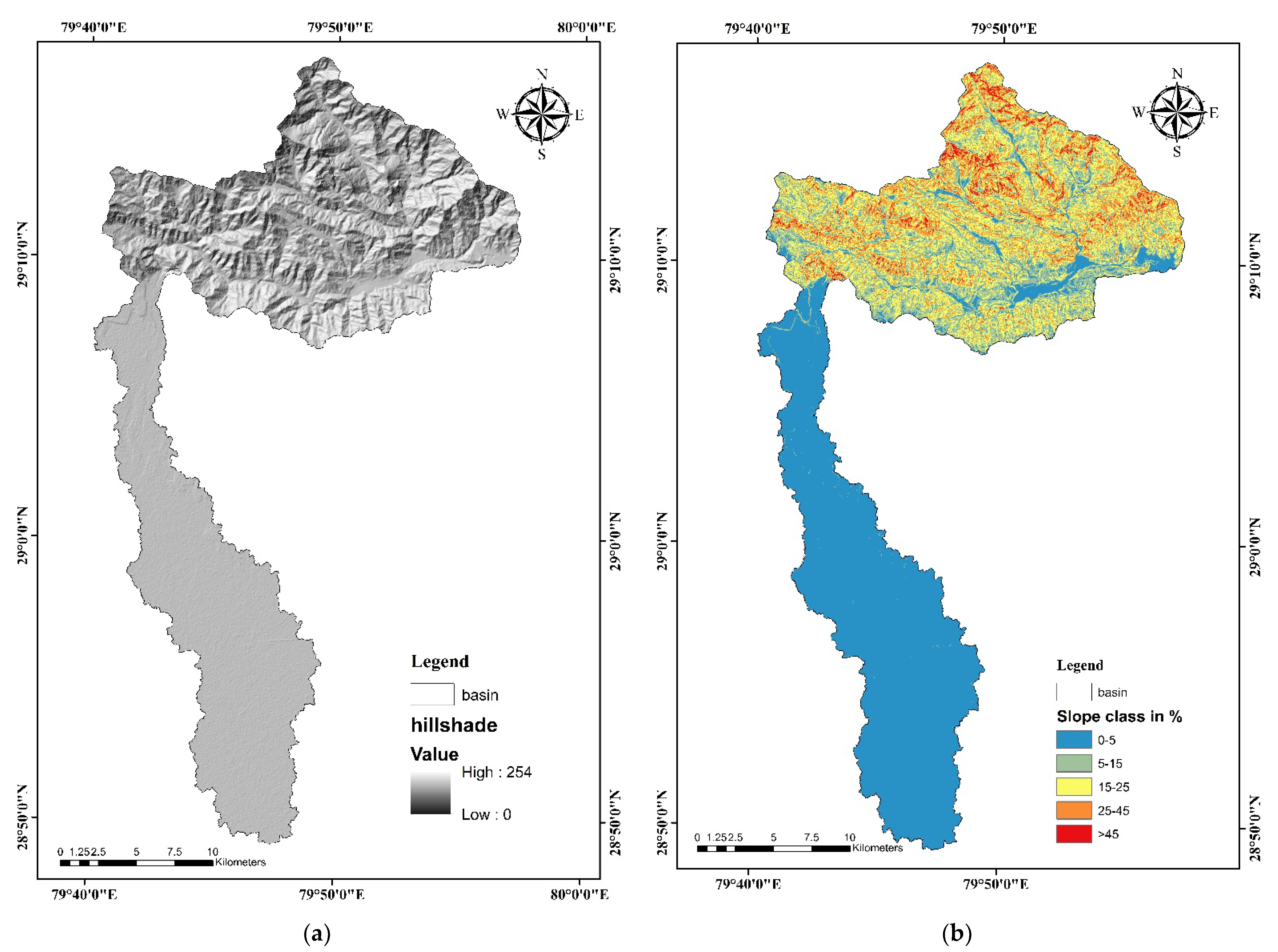
3.6.1. Hillshade Map

A hillshade map is a 3D representation of a surface. It is generally rendered in greyscale. The elevation and all 3D information about the terrain are contained in the DEM raster file. The hillshade map was generated using the Spatial Analyst Tool in ArcGIS v10.4.1 (Raster → Surface → Hillshade). The hillshade map is shown in Figure 10a, and their values were 0–254.

3.6.2. Slope Map

Figure 10b depicts the study area’s slope map. The raster properties and the resulting raster file were used to categorize five slope classes, as shown in

Table 6. Classification of land slope in Nandhour-Kailash River watershed.

S. No.	Slope Class	Land Slope (%)	Area (km2)
1	A (Little or No slope)	0–5	120.94
2	B (Gentle)	5–15	97.09
3	C (Moderate)	15–25	25.81
4	D (Steep)	25–45	86.38

, namely, little or no slope (0–5%), gentle (5–15%), moderate (15–25%), steep (25–45%), and extremely steep (>45%), with an area of 120.94 km², 97.09 km², 25.81 km², 86.38 km², and 143.87 km², respectively. The maximum area of the slope class (0–5%) was 25.51%, while the minimum area (15–25%) was 5.44%. About 45.99% of the Nandhour-Kailash River watershed was found to have a 15% slope.

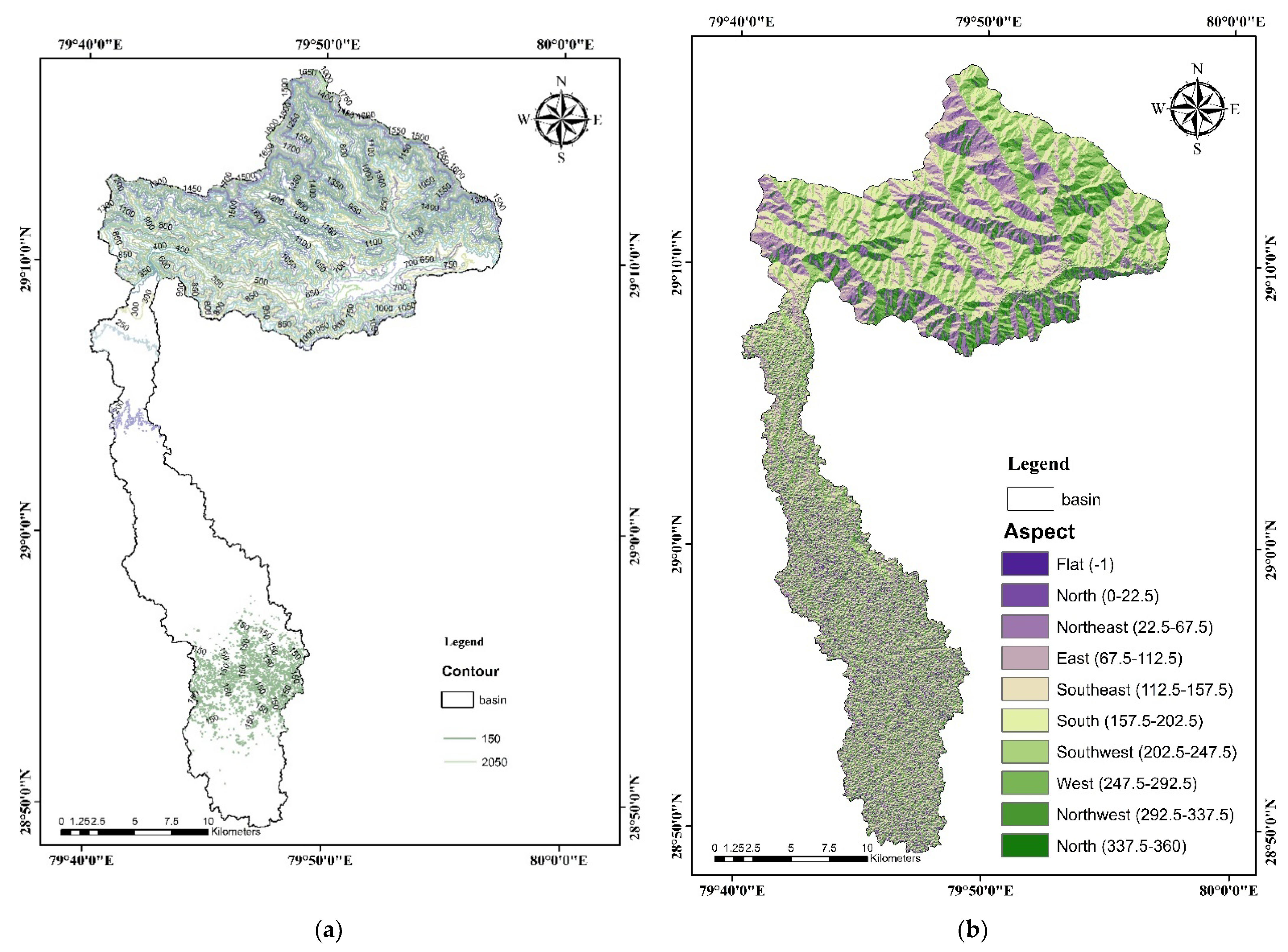
3.6.3. Contour Map

A topographic map shows a contour line to indicate ground elevation or depression. The contour map was created using DEM and ArcGIS v 10.4.1 software to create contours of various elevations, using the Spatial Analyst Tool (Raster → Surface → Contour) at 50 m intervals. The contour elevation ranged between 150 and 2050 m above mean sea level, as shown in Figure 11a.

3.6.4. Aspect Map

The slope’s terrain aspect is determined by the compass direction it faces. The azimuth is indicated by 0 to 360 degrees measured from the north. The north aspect generally has more moisture and is richer in vegetation. In contrast, the south aspect has more sunlight, resulting in drier conditions and sparse vegetation. With the help of the DEM raster and Spatial Analyst Tool in ArcGIS v10.4.1 (Raster → Surface → Aspect → Reclass → Reclassify), the aspect map of the study area was produced. It is shown in Figure 11b, and the geographical extent of various aspect classes is presented in

Table 7. The geographical extent of different aspect classes in the Nandhour-Kailash River watershed.

S. No.	Aspect	Area (km2)	Area (%)
1	Flat (−1°)	16.67	3.52
2	North (0°–22.5°)	29.91	6.31
3	North–East (22.5°–67.5°)	57.17	12.06
4	East (67.5°–112.5°)	52.24	11.02
5	South–East (112.5°–157.5°)	62.36	13.15
6	South (157.5°–202.5°)	64.02	13.50
7	South–West (202.5°–247.5°)	72.45	15.28
8	West (247.5°–292.5°)	53.35	11.25
9	North–West (292.5°–337.5°)	47.75	10.07
10	North (337.5°–360°)	18.17	3.83

. The south–west aspect covered a maximum area of 72.45 km² (15.28%), while the flat aspect had a minimum area of 16.31 km² (3.52%).

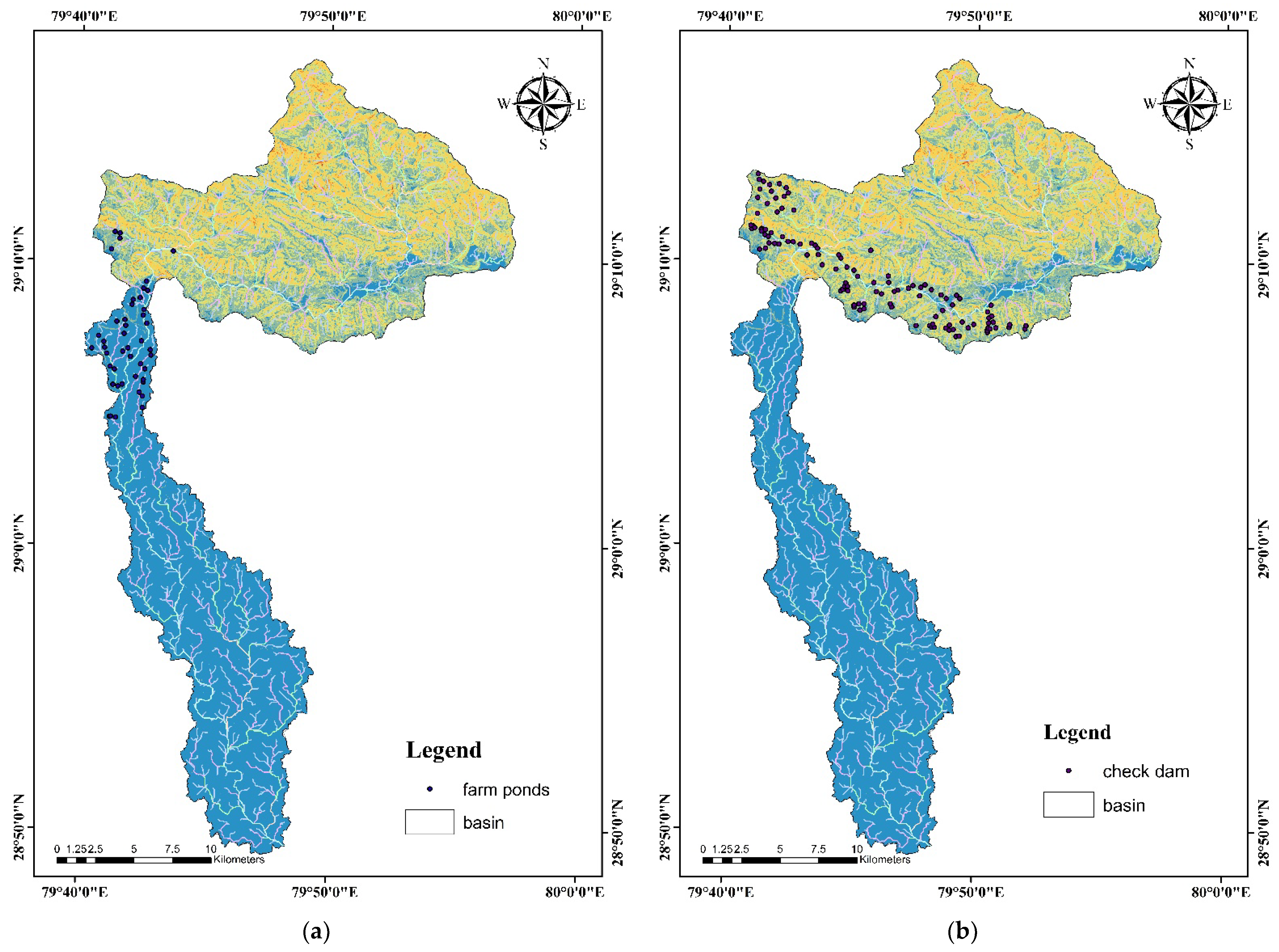
3.7. Identification of Potential Sites for Artificial Groundwater Recharge

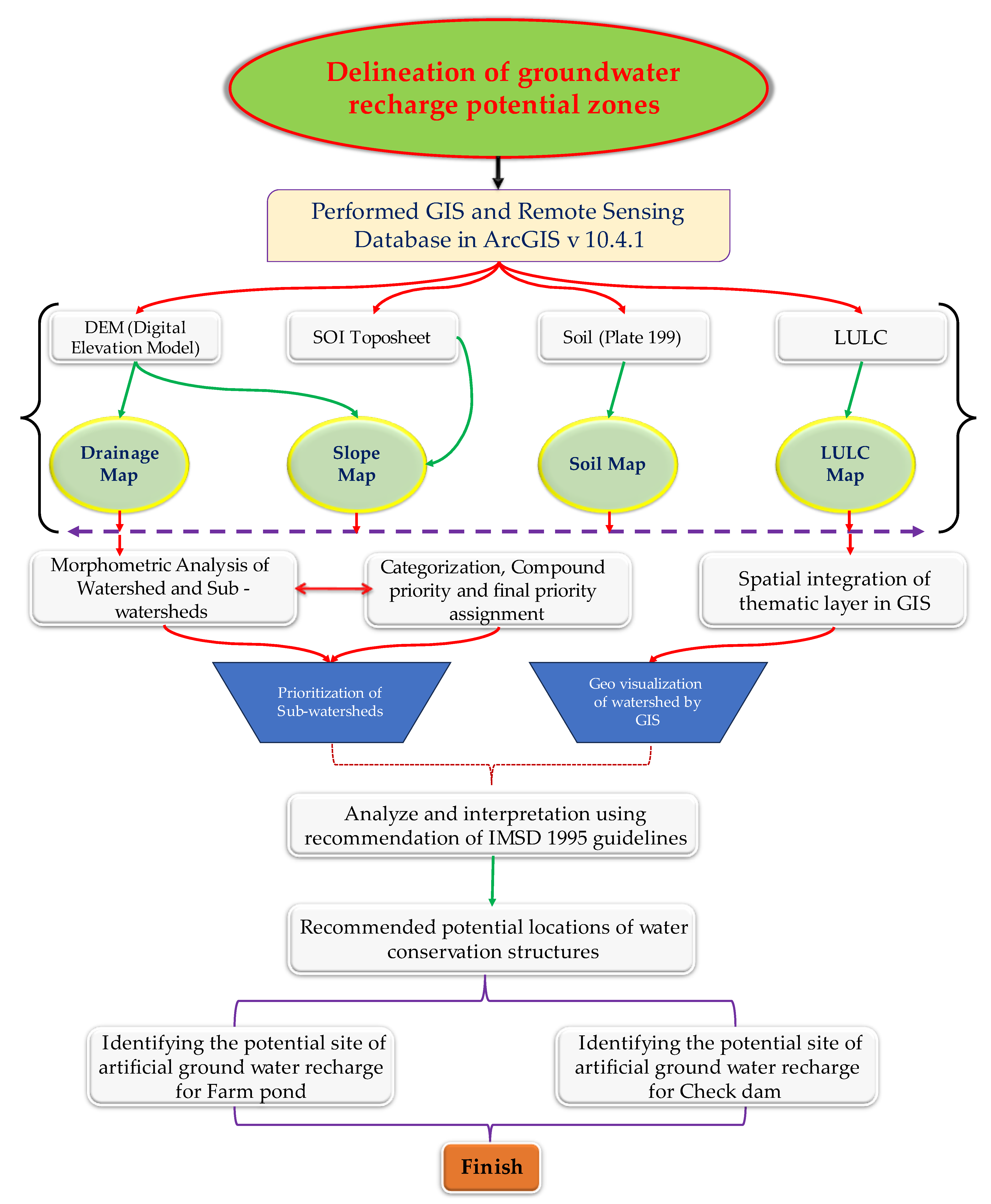
It is recommended that the recharge structures should be constructed in a high infiltration zone. In contrast, water harvesting structures must be in soil with low infiltration zones. Thus, the recharge structures were recommended in the Bhabar zone. The geo-visualization concept was used to pinpoint potential locations for artificial groundwater recharge structures. Thematic maps of soil, slope, drainage, and LULC were superimposed in ArcGIS 10.4.1. The sites were visualized following the priority set for identifying potential zones in the watershed area. The proposed recharge sites were divided into farm ponds and check dams per the Integrated Mission for Sustainable Development (IMSD) guidelines [82]. The reason for the choice of criteria for their location is the location of recharge sites depending on the terrain (slope) only. A simple and practical approach to managing watersheds can be achieved by identifying potential groundwater zones and suitable sites for artificial ground recharge. A typical structure of farm ponds and check dams is shown in Supplementary Figure S5.

Decision rules: The following rules/guidelines of IMSD (1995) were followed while identifying potential sites:

(a)

Farm ponds: This structure could be constructed on a first-order stream with a 0–5% land slope. Suitable farm pond sites were identified (Figure 12a), and 36 potential sites (

Table 8. The area is suitable for check dams and farm ponds in the Nandhour-Kailash River watershed.

Type of Structure	Slope (%)	Area (km2)	Number of Potential Sites
Farm ponds	0–5	120.94	36
Check dams	<15	218.03	105

) for constructing farm ponds, covering an area of 120.94 km², were identified.

(b)

Check dams: Check dams could be built in the first to fourth stream order on land with a <15% slope. Suitable check dam sites were identified (Figure 12b). The area ideal for constructing 105 check dams (Table 8) in the Nandhour-Kailash River watershed was 218.03 km².

Farm ponds are small to medium-sized water bodies typically found on agricultural properties. These man-made or natural depressions are designed to capture and store rainwater, runoff, or groundwater, serving several crucial purposes, such as water storage, irrigation, livestock watering, erosion control, and fish farming. In modern farming, a typical farm pond is a shallow, rectangular, or circular body of water ranging in size from a fraction of an acre to several acres. Farm ponds are essential to sustainable agriculture, promoting water conservation, soil protection, and enhanced crop and livestock management. They are adaptable to various agricultural settings and are a valuable resource for farmers worldwide.

Check dams in India are small to medium-sized structures built across rivers, streams, and seasonal watercourses. These dams slow water flow and capture sediment and debris while allowing excess water to percolate into the ground. Check dams are essential for several reasons: soil and water conservation, groundwater recharge, irrigation, and drinking water supply, among others. Check dams in India are vital in water resource management, especially in regions prone to water scarcity and soil erosion. These structures contribute to sustainable agriculture, provide access to clean drinking water, and mitigate the impact of floods, ultimately improving the lives of local communities.

A combination of environmental, agricultural, and socio-economic factors influences the choice of criteria for implementing farm ponds and check dams. These criteria are selected to address specific regional or local needs and to ensure the effective utilization of these water management structures. The primary reason for establishing criteria for farm ponds and check dams is the land slope, as mentioned in the Integrated Mission for Sustainable Development (IMSD) guidelines [82].

From the geological aspect, the soil map has been analyzed in the current study. The areas with more soil erosion are suggested for soil and water conservation, mainly considering the role of terrain topographic features and land use. Landscape patterns and hydrology-based extractions of stream patterns in the study area are sufficient to solve the purpose of the current study. However, lithology and lineaments can also be considered as part of future modeling for assessing their impact on site selection for ponds, dykes, and check dams. The geological nature of aquifers plays an essential role in selecting particular types of ponds, dykes, and check dams.

4. Discussion

Groundwater is a crucial natural resource to provide water supply to people worldwide. It is a valuable and frequently abundant resource. It has evolved as a significant water supply for various sectors, including irrigation, households, and industries. Groundwater levels have significantly decreased in many areas of India due to indiscriminate use and over-exploitation. According to several regional groundwater studies, Udham Singh Nagar district and adjoining areas of Uttar Pradesh also suffer from a successive decline in the groundwater table [84,85,86]. Many blocks of adjoining areas of Uttar Pradesh have already been declared “over-exploited or dark zone” due to excessive groundwater withdrawal and the water table’s decline. Aquifers in the Tarai area of Uttarakhand and surrounding areas of Uttar Pradesh receive natural groundwater recharge in the Kumaon region’s Bhabar area. To recharge the region’s aquifers, there is an urgent need to identify possible sites in the recharging zones to construct recharging structures. Therefore, this study was conducted in the Nandhour-Kailash River watershed with the goals of morphometric analysis (linear, areal, and relief aspects) of the watershed, prioritization of sub-watersheds based on morphometric parameters, and identification of potential artificial groundwater recharge site in the study area. This was done to improve, develop, and manage the regional groundwater resources and identify suitable sites for groundwater recharge.

The use of remote-sensing techniques and picture interpretations can be very economically advantageous and have the potential to help decipher hydrological surveys. These modern techniques enable pre-investment reconnaissance mapping and terrain analysis of water resources with greater accuracy, flexibility, and speed so that any hydrological survey can be conducted quicker, with reduced cost and greater precision. This study will also benefit future groundwater aquifer investigations that will be performed using geophysical methods to delineate their exact locations. An excellent way of finding potential recharge areas is remote sensing and GIS [19,20,87], using different techniques, which is a perfect way to do so [9,36,88,89,90,91,92]. None of the previous experiments on identifying artificial groundwater recharge potential zones have been conducted in this watershed. It is known that the groundwater table is depleting every year, so it will be beneficial to identify artificial groundwater recharge zones with rainwater. Chowdary et al. [93] and Chauhan et al. [94] used the Integrated Mission for Sustainable Development (IMSD) guideline and slope criteria to find out the potential groundwater recharge zone with suitable water harvesting structures.

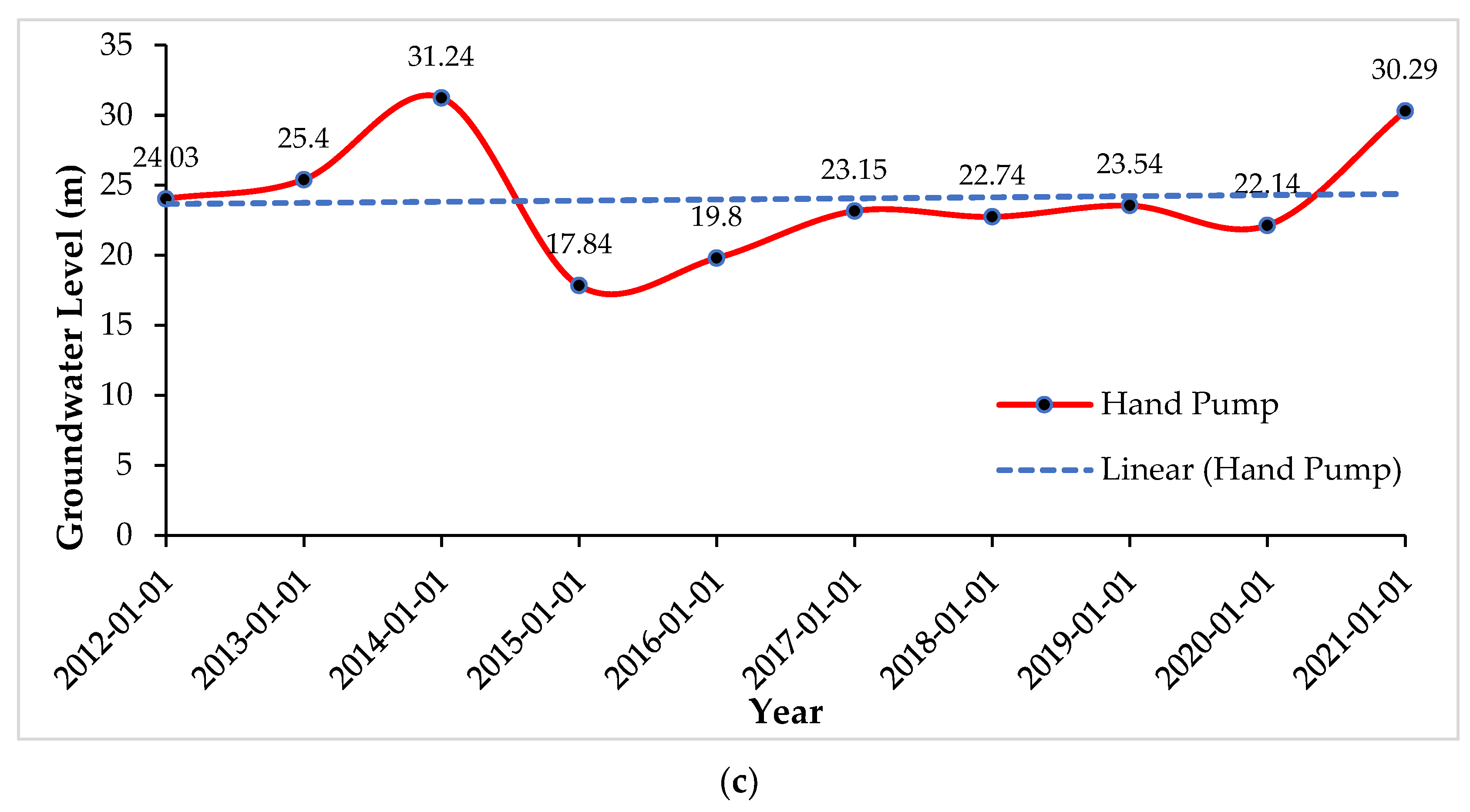
Deoli and Kumar [84] stated that the groundwater level fluctuation in the Terai region of the Kumaon division sharply decreased from 2002 to 2016. The trend is negative for this study period in all months, and we found that the average groundwater table fluctuation was 10.47 cm from 2002–2016. Biswas et al. (2018) found that the groundwater table is declining yearly by 0.228 and 0.267 m/year during pre- and post-monsoon seasons in the Agra Uttar Pradesh region. Dey et al. [85] reported a decreasing trend in water table fluctuation for the Varanasi district in Uttar Pradesh in the recent decade. Many other researchers have reported that groundwater levels in most wells show a declining trend. This increasing trend is a severe concern for groundwater resource assessment and its management for sustainable development [95,96,97]. The potential locations for artificial groundwater recharge were identified using the geo-visualization concept. The locations of recharge sites in the watershed area were identified by overlaying soil maps, drainage maps, slope maps, and land use/land cover maps. Based on the conditions and IMSD (1995) guidelines, the locations for the recharge sites were recommended for two types of water recharging structures, i.e., farm ponds and check dams. Potential sites for artificial groundwater recharge zones with 0–5 and <15% land slope for farm ponds and check dams, respectively, are indicated by the solid black color circle in Figure 12. No studies have been conducted on this watershed to identify a potential groundwater recharge zone, nor was the groundwater recharge evaluated or monitored, making it impossible to discuss validating the identified location using actual experimentation data collected in the past.

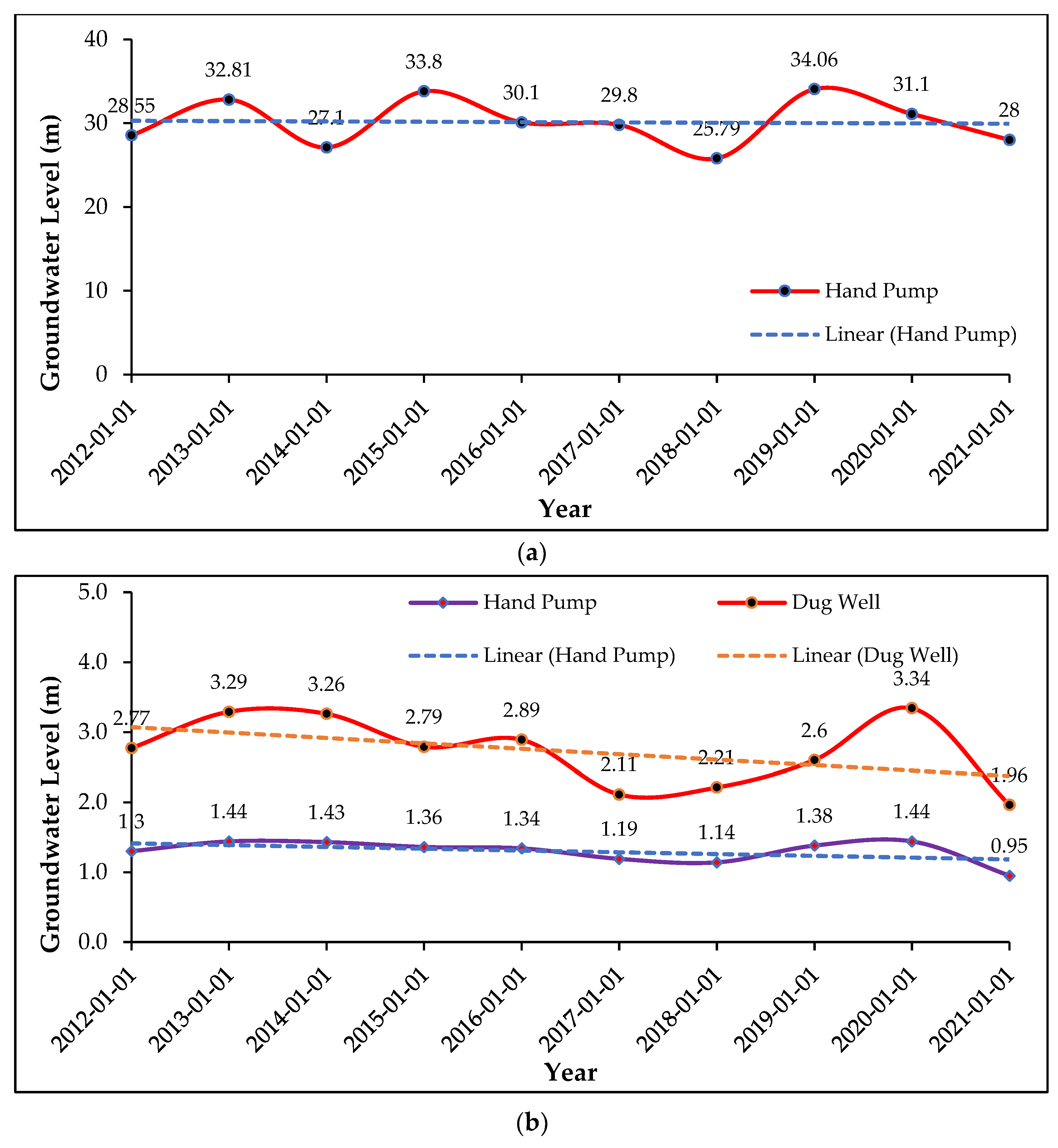
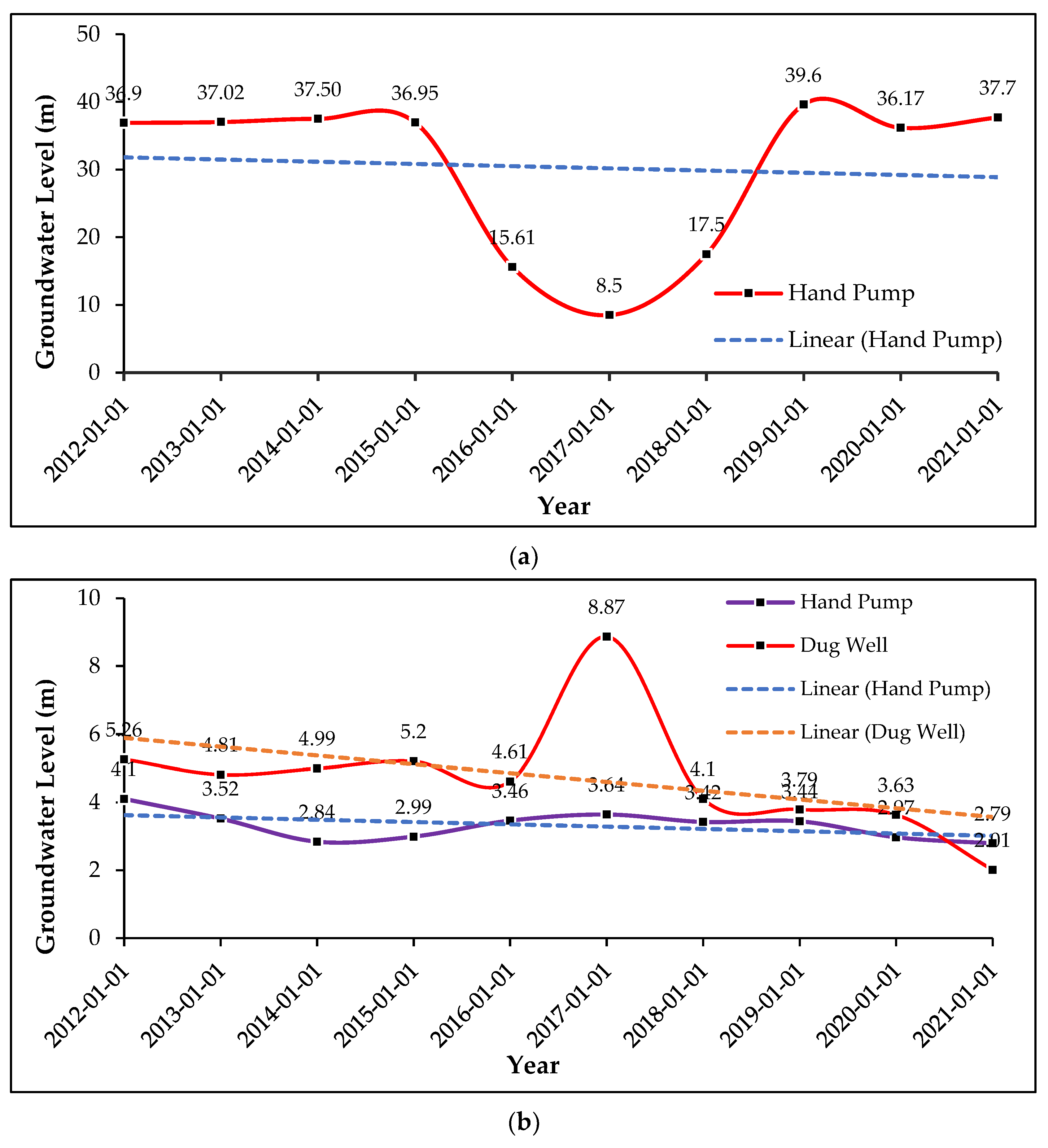
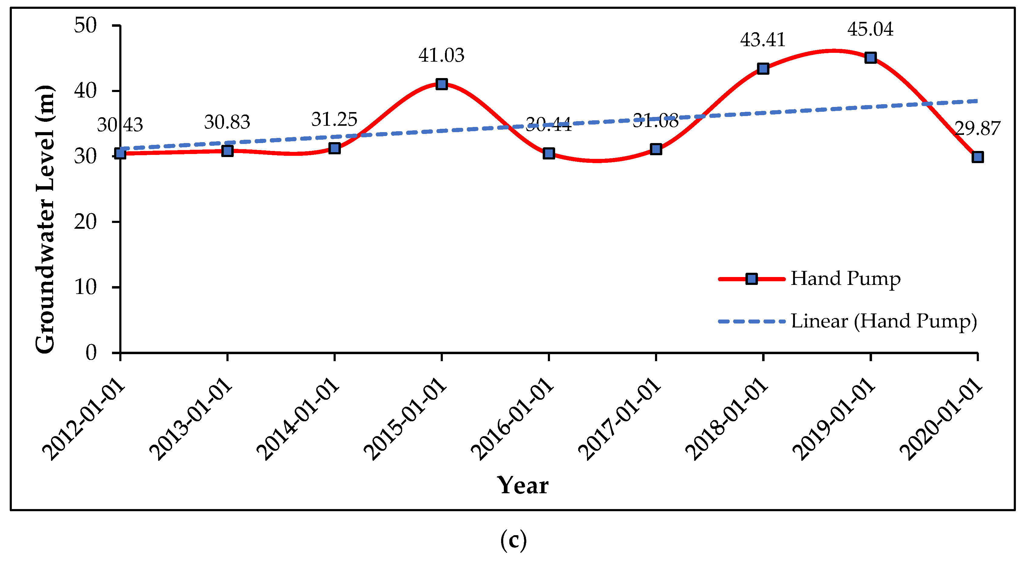
A comprehensive validation process was conducted for the well data within the study area. To accomplish this, we divided the study area into distinct blocks, and within each of these blocks, we employed K-means clustering based on the similarity of groundwater levels. This clustering approach allowed us to group wells with similar groundwater level patterns, providing valuable insight into the spatial distribution of groundwater characteristics within the study area. To further confirm the validity of our results, we employed graphical representations (Figure 13 and Figure 14). By plotting groundwater level data on graphs, we could visually depict the changes in groundwater levels across the study area. These visual representations demonstrated a clear and concerning trend: the groundwater table was declining in different districts or regions within the study area. This finding is significant for groundwater management and suggests that various factors may be at play, such as changes in water usage, climate variations, or geological influences, contributing to the observed decline in groundwater levels. Understanding these trends is crucial for effective groundwater resource management and sustainability efforts within the study area.

The Nature of Groundwater in the Nandhaur-Kailash River watershed is primarily derived from rainfall and surface water sources. Rainwater percolates through the soil and rock layers, replenishing the aquifers below. The area’s geology plays a crucial role in determining the nature of the groundwater, with different aquifers varying in permeability, depth, and water quality. The groundwater depth in the watershed can vary significantly depending on the location, geological conditions, and the seasonal variation in rainfall. The depth of pre- and post-monsoon groundwater levels in the Nandhaur-Kailash River watershed is shown in Figure 13 and Figure 14. The water table may be relatively shallow in areas with sufficient recharge and porous geological formations.

In contrast, regions with less rainfall and impermeable rock layers may have deeper groundwater tables. The groundwater depth can change due to climatic variations and human water extraction activities. Seasonal variations in rainfall significantly impact groundwater levels. During the monsoon season, groundwater recharge is more substantial, leading to higher water tables. Conversely, groundwater levels may drop in drier months due to increased pumping and reduced recharge. Several factors, including geological structures, topography, and human activities, influence groundwater circulation in the Nandhaur-Kailash River watershed. The movement of groundwater is typically slow, governed by the permeability of the subsurface materials. In this region, groundwater may flow toward rivers and streams, which act as natural discharge points. The circulation is also affected by human abstraction for irrigation, drinking water, and industrial use, which can alter the natural flow patterns.

5. Conclusions

This study demonstrates the practical application of remote sensing and GIS methodologies to prioritize sub-watersheds by evaluating morphometric attributes, conducting land use and land cover analysis, classifying soil and slope, and performing terrain analysis across 12 sub-watersheds within the Nandhour-Kailash River watershed. Additionally, the study identifies suitable locations for artificial groundwater recharge. The study of the Nandhour-Kailash River watershed led to the following conclusions:

i.

The dendritic drainage pattern and extremely rough drainage texture were present in the Nandhour-Kailash River watershed. The study area’s bifurcation ratio (R_b) value demonstrated that the geologic structures do not impact the drainage pattern.

ii.

The value of drainage texture (T), length of overland flow (L_g), and elongation ratio (R_e) suggested that the watershed had a moderate drainage texture, a high length of overland flow, and an elongated shape, respectively. The watershed had an elongated shape with lower peak flows of longer duration, a lower peak of flow, and less elongation with increased erosion, according to the values of the circulatory ratio (R_c), form factor (F_f), and compactness coefficient (C_c).

iii.

Two sub-watersheds (SWS11, SWS12) were found under high priority and require immediate attention for soil and water conservation. Five sub-watersheds (SWS4, SWS5, SWS8, SWS9, SWS10) were considered moderate soil erosion and land degradation under medium priority. Another five sub-watersheds (SWS1, SWS2, SWS3, SWS6, SWS7) were under low priority, indicating a low risk of soil erosion and degradation.

iv.

About 45.99% of the Nandhour-Kailash River watershed has less than a 15% slope. The maximum area of the south–west aspect was 15.28%, while the flat aspect occupied a minimum area of 3.52%.

v.

The suitable locations of 36 farm ponds were suggested on the first-order stream in a 120.94 km² area, having a land slope of 0–5%. In contrast, 105 check dams were suggested on the first to fourth-order streams with 218.03 km² area having a land slope of <15% as they were recognized as possible sites for artificial groundwater recharge based on the conditions and guidelines of IMSD (1995).

According to the results of this study, concurrent analysis of massive data sets and decision-making for groundwater studies in watersheds could be facilitated by RS. GIS techniques and tools are more efficient and cost-effective and provide adequate support. The integrated map could be instructive for various tasks, such as sustainable groundwater development and determining priority areas for implementing regional water conservation projects and programs. The Nandhour-Kailash River watershed has successfully applied GIS and RS techniques to assess groundwater potentiality. The mapping of the potential groundwater recharge zones is especially beneficial for the Government departments and NGOs to require suitable and effective take-up for soil and water conservation measures in the area.

This study holds significant global relevance as it can be applied to various regions worldwide, each facing unique water resource management challenges. In arid and semi-arid regions, such as parts of North Africa or the southwestern United States, identifying suitable sites for groundwater recharge is essential for mitigating water scarcity issues. In contrast, in densely populated urban areas, where groundwater depletion and land constraints are pressing concerns, this study can aid in optimizing existing resources. To improve future studies, researchers can enhance the accuracy of site selection by incorporating advanced satellite imagery and machine learning algorithms. Additionally, collaboration between experts from various regions can lead to developing a more comprehensive and adaptable methodology, considering the specific environmental and socio-economic factors influencing groundwater recharge potential. This would enable a more effective and globally applicable approach to artificial groundwater recharge.

References

1. Selvakumar, S.; Chandrasekar, N.; Kumar, G. Hydrogeochemical Characteristics and Groundwater Contamination in the Rapid Urban Development Areas of Coimbatore, India. Water Resour. Ind. 2017, 17, 26–33. [Google Scholar] [CrossRef]
2. Sinha, D.D.; Mohapatra, S.N.; Pani, P. Mapping and Assessment of Groundwater Potential in Bilrai Watershed (Shivpuri District, M.P.)—A Geomatics Approach. J. Indian Soc. Remote Sens. 2012, 40, 649–668. [Google Scholar] [CrossRef]
3. Alrawi, I.; Chen, J.; Othman, A.A. Groundwater Potential Zone Mapping: Integration of Multi-Criteria Decision Analysis (MCDA) and GIS Techniques for the Al-Qalamoun Region in Syria. ISPRS Int. J. Geo-Inf. 2022, 11, 603. [Google Scholar] [CrossRef]
4. Jaiswal, R.K.; Mukherjee, S.; Krishnamurthy, J.; Saxena, R. Role of Remote Sensing and GIS Techniques for Generation of Groundwater Prospect Zones towards Rural Development--an Approach. Int. J. Remote Sens. 2003, 24, 993–1008. [Google Scholar] [CrossRef]
5. Ndhlovu, G.Z.; Woyessa, Y.E. Integrated Assessment of Groundwater Potential Using Geospatial Techniques in Southern Africa: A Case Study in the Zambezi River Basin. Water 2021, 13, 2610. [Google Scholar] [CrossRef]
6. Hamdy, A.; Ragab, R.; Scarascia-Mugnozza, E. Coping with Water Scarcity: Water Saving and Increasing Water Productivity. Irrig. Drain. 2003, 52, 3–20. [Google Scholar] [CrossRef]
7. Rosegrant, M.W.; Cai, X. Global Water Demand and Supply Projections. Water Int. 2002, 27, 170–182. [Google Scholar] [CrossRef]
8. Yeh, H.-F.; Cheng, Y.-S.; Lin, H.-I.; Lee, C.-H. Mapping Groundwater Recharge Potential Zone Using a GIS Approach in Hualian River, Taiwan. Sustain. Environ. Res. 2016, 26, 33–43. [Google Scholar] [CrossRef]
9. Arefin, R. Groundwater Potential Zone Identification at Plio-Pleistocene Elevated Tract, Bangladesh: AHP-GIS and Remote Sensing Approach. Groundw. Sustain. Dev. 2020, 10, 100340. [Google Scholar] [CrossRef]
10. Hammami, S.; Zouhri, L.; Souissi, D.; Souei, A.; Zghibi, A.; Marzougui, A.; Dlala, M. Application of the GIS Based Multi-Criteria Decision Analysis and Analytical Hierarchy Process (AHP) in the Flood Susceptibility Mapping (Tunisia). Arab. J. Geosci. 2019, 12, 653. [Google Scholar] [CrossRef]
11. Panahi, M.R.; Mousavi, S.M.; Rahimzadegan, M. Delineation of Groundwater Potential Zones Using Remote Sensing, GIS, and AHP Technique in Tehran–Karaj Plain, Iran. Environ. Earth Sci. 2017, 76, 792. [Google Scholar] [CrossRef]
12. Singh, L.K.; Jha, M.K.; Chowdary, V.M. Multi-Criteria Analysis and GIS Modeling for Identifying Prospective Water Harvesting and Artificial Recharge Sites for Sustainable Water Supply. J. Clean. Prod. 2017, 142, 1436–1456. [Google Scholar] [CrossRef]
13. Mahmoud, S.H.; Alazba, A.A. The Potential of in Situ Rainwater Harvesting in Arid Regions: Developing a Methodology to Identify Suitable Areas Using GIS-Based Decision Support System. Arab. J. Geosci. 2015, 8, 5167–5179. [Google Scholar] [CrossRef]
14. Dillon, P. Future Management of Aquifer Recharge. Hydrogeol. J. 2005, 13, 313–316. [Google Scholar] [CrossRef]
15. Jackson, T.J. Remote Sensing of Soil Moisture: Implications for Groundwater Recharge. Hydrogeol. J. 2002, 10, 40–51. [Google Scholar] [CrossRef]
16. Ibrahim-Bathis, K.; Ahmed, S.A. Geospatial Technology for Delineating Groundwater Potential Zones in Doddahalla Watershed of Chitradurga District, India. Egypt. J. Remote Sens. Sp. Sci. 2016, 19, 223–234. [Google Scholar] [CrossRef]
17. Nhu, V.-H.; Rahmati, O.; Falah, F.; Shojaei, S.; Al-Ansari, N.; Shahabi, H.; Shirzadi, A.; Górski, K.; Nguyen, H.; Ahmad, B. Mapping of Groundwater Spring Potential in Karst Aquifer System Using Novel Ensemble Bivariate and Multivariate Models. Water 2020, 12, 985. [Google Scholar] [CrossRef]
18. Ardakani, A.H.H.; Shojaei, S.; Siasar, H.; Ekhtesasi, M.R. Heuristic Evaluation of Groundwater in Arid Zones Using Remote Sensing and Geographic Information System. Int. J. Environ. Sci. Technol. 2020, 17, 633–644. [Google Scholar] [CrossRef]
19. Ardakani, A.H.H.; Shojaei, S.; Shahvaran, A.R.; Kalantari, Z.; Cerdà, A.; Tiefenbacher, J. Selecting Potential Locations for Groundwater Recharge by Means of Remote Sensing and GIS and Weighting Based on Boolean Logic and Analytic Hierarchy Process. Environ. Earth Sci. 2022, 81, 8. [Google Scholar] [CrossRef]
20. Bera, A.; Mukhopadhyay, B.P.; Barua, S. Delineation of Groundwater Potential Zones in Karha River Basin, Maharashtra, India, Using AHP and Geospatial Techniques. Arab. J. Geosci. 2020, 13, 693. [Google Scholar] [CrossRef]
21. Singh, A.; Panda, S.N.; Kumar, K.S.; Sharma, C.S. Artificial Groundwater Recharge Zones Mapping Using Remote Sensing and GIS: A Case Study in Indian Punjab. Environ. Manag. 2013, 52, 61–71. [Google Scholar] [CrossRef] [PubMed]
22. Solomon, S.; Quiel, F. Groundwater Study Using Remote Sensing and Geographic Information Systems (GIS) in the Central Highlands of Eritrea. Hydrogeol. J. 2006, 14, 1029–1041. [Google Scholar] [CrossRef]
23. Singh, C.K.; Shashtri, S.; Singh, A.; Mukherjee, S. Quantitative Modeling of Groundwater in Satluj River Basin of Rupnagar District of Punjab Using Remote Sensing and Geographic Information System. Environ. Earth Sci. 2011, 62, 871–881. [Google Scholar] [CrossRef]
24. Mukherjee, P.; Singh, C.K.; Mukherjee, S. Delineation of Groundwater Potential Zones in Arid Region of India—A Remote Sensing and GIS Approach. Water Resour. Manag. 2012, 26, 2643–2672. [Google Scholar] [CrossRef]
25. Zghibi, A.; Mirchi, A.; Msaddek, M.H.; Merzougui, A.; Zouhri, L.; Taupin, J.-D.; Chekirbane, A.; Chenini, I.; Tarhouni, J. Using Analytical Hierarchy Process and Multi-Influencing Factors to Map Groundwater Recharge Zones in a Semi-Arid Mediterranean Coastal Aquifer. Water 2020, 12, 2525. [Google Scholar] [CrossRef]
26. Allafta, H.; Opp, C.; Patra, S. Identification of Groundwater Potential Zones Using Remote Sensing and GIS Techniques: A Case Study of the Shatt Al-Arab Basin. Remote Sens. 2020, 13, 112. [Google Scholar] [CrossRef]
27. Ahmed, A.; Ranasinghe-Arachchilage, C.; Alrajhi, A.; Hewa, G. Comparison of Multicriteria Decision-Making Techniques for Groundwater Recharge Potential Zonation: Case Study of the Willochra Basin, South Australia. Water 2021, 13, 525. [Google Scholar] [CrossRef]
28. Assaf, H.; Saadeh, M. Geostatistical Assessment of Groundwater Nitrate Contamination with Reflection on DRASTIC Vulnerability Assessment: The Case of the Upper Litani Basin, Lebanon. Water Resour. Manag. 2009, 23, 775–796. [Google Scholar] [CrossRef]
29. Hoffmann, J.; Sander, P. Remote Sensing and GIS in Hydrogeology. Hydrogeol. J. 2007, 15, 1–3. [Google Scholar] [CrossRef]
30. Dinesh Kumar, P.K.; Gopinath, G.; Seralathan, P. Application of Remote Sensing and GIS for the Demarcation of Groundwater Potential Zones of a River Basin in Kerala, Southwest Coast of India. Int. J. Remote Sens. 2007, 28, 5583–5601. [Google Scholar] [CrossRef]
31. Srivastava, P.K.; Bhattacharya, A.K. Groundwater Assessment through an Integrated Approach Using Remote Sensing, GIS and Resistivity Techniques: A Case Study from a Hard Rock Terrain. Int. J. Remote Sens. 2006, 27, 4599–4620. [Google Scholar] [CrossRef]
32. Sreedevi, P.D.; Subrahmanyam, K.; Ahmed, S. Integrated Approach for Delineating Potential Zones to Explore for Groundwater in the Pageru River Basin, Cuddapah District, Andhra Pradesh, India. Hydrogeol. J. 2005, 13, 534–543. [Google Scholar] [CrossRef]
33. Nag, S.K. Application of Lineament Density and Hydrogeomorphology to Delineate Groundwater Potential Zones of Baghmundi Block in Purulia District, West Bengal. J. Indian Soc. Remote Sens. 2005, 33, 521–529. [Google Scholar] [CrossRef]
34. Chenini, I.; Mammou, A.B.; El May, M. Groundwater Recharge Zone Mapping Using GIS-Based Multi-Criteria Analysis: A Case Study in Central Tunisia (Maknassy Basin). Water Resour. Manag. 2010, 24, 921–939. [Google Scholar] [CrossRef]
35. Saraf, A.K.; Choudhury, P.R. Integrated Remote Sensing and GIS for Groundwater Exploration and Identification of Artificial Recharge Sites. Int. J. Remote Sens. 1998, 19, 1825–1841. [Google Scholar] [CrossRef]
36. Jasrotia, A.S.; Kumar, R.; Saraf, A.K. Delineation of Groundwater Recharge Sites Using Integrated Remote Sensing and GIS in Jammu District, India. Int. J. Remote Sens. 2007, 28, 5019–5036. [Google Scholar] [CrossRef]
37. Maksud Kamal, A.S.M.; Midorikawa, S. GIS-Based Geomorphological Mapping Using Remote Sensing Data and Supplementary Geoinformation. Int. J. Appl. Earth Obs. Geoinf. 2004, 6, 111–125. [Google Scholar] [CrossRef]
38. Gustavsson, M.; Kolstrup, E.; Seijmonsbergen, A.C. A New Symbol-and-GIS Based Detailed Geomorphological Mapping System: Renewal of a Scientific Discipline for Understanding Landscape Development. Geomorphology 2006, 77, 90–111. [Google Scholar] [CrossRef]
39. Singh, A.K.; Parkash, B.; Choudhury, P.R. Integrated Use of SRM, Landsat ETM+ Data and 3D Perspective Views to Identify the Tectonic Geomorphology of Dehradun Valley, India. Int. J. Remote Sens. 2007, 28, 2403–2414. [Google Scholar] [CrossRef]
40. Chowdhury, A.; Jha, M.K.; Chowdary, V.M.; Mal, B.C. Integrated Remote Sensing and GIS-based Approach for Assessing Groundwater Potential in West Medinipur District, West Bengal, India. Int. J. Remote Sens. 2009, 30, 231–250. [Google Scholar] [CrossRef]
41. Santha Sophiya, M.; Syed, T.H. Assessment of Vulnerability to Seawater Intrusion and Potential Remediation Measures for Coastal Aquifers: A Case Study from Eastern India. Environ. Earth Sci. 2013, 70, 1197–1209. [Google Scholar] [CrossRef]
42. Nagaraju, D.; Nassery, H.R.; Adinehvandi, R. Determine Suitable Sites for Artificial Recharge Using Hierarchical Analysis (AHP), Remote Sensing (RS) and Geographic Information Systems (GIS). Int. J. Earth Sci. Eng. 2012, 5, 1328–1335. [Google Scholar]
43. Agarwal, E.; Agarwal, R.; Garg, R.D.; Garg, P.K. Delineation of Groundwater Potential Zone: An AHP/ANP Approach. J. Earth Syst. Sci. 2013, 122, 887–898. [Google Scholar] [CrossRef]
44. Agarwal, R.; Garg, P.K.; Garg, R.D. Remote Sensing and GIS Based Approach for Identification of Artificial Recharge Sites. Water Resour. Manag. 2013, 27, 2671–2689. [Google Scholar] [CrossRef]
45. Sarkar, P.; Kumar, P.; Vishwakarma, D.K.; Ashok, A.; Elbeltagi, A.; Gupta, S.; Kuriqi, A. Watershed Prioritization Using Morphometric Analysis by MCDM Approaches. Ecol. Inform. 2022, 70, 101763. [Google Scholar] [CrossRef]
46. Kumar, P.; Sarkar, P. A Comparison of the AHP and TOPSIS Multi-Criteria Decision-Making Tools for Prioritizing Sub-Watersheds Using Morphometric Parameters’ Analysis. Model. Earth Syst. Environ. 2022, 8, 3973–3983. [Google Scholar] [CrossRef]
47. Ravi Shankar, M.N.; Mohan, G. A GIS Based Hydrogeomorphic Approach for Identification of Site-Specific Artificial-Recharge Techniques in the Deccan Volcanic Province. J. Earth Syst. Sci. 2005, 114, 505–514. [Google Scholar] [CrossRef]
48. Oh, H.-J.; Kim, Y.-S.; Choi, J.-K.; Park, E.; Lee, S. GIS Mapping of Regional Probabilistic Groundwater Potential in the Area of Pohang City, Korea. J. Hydrol. 2011, 399, 158–172. [Google Scholar] [CrossRef]
49. Manap, M.A.; Nampak, H.; Pradhan, B.; Lee, S.; Sulaiman, W.N.A.; Ramli, M.F. Application of Probabilistic-Based Frequency Ratio Model in Groundwater Potential Mapping Using Remote Sensing Data and GIS. Arab. J. Geosci. 2014, 7, 711–724. [Google Scholar] [CrossRef]
50. Razandi, Y.; Pourghasemi, H.R.; Neisani, N.S.; Rahmati, O. Application of Analytical Hierarchy Process, Frequency Ratio, and Certainty Factor Models for Groundwater Potential Mapping Using GIS. Earth Sci. Inform. 2015, 8, 867–883. [Google Scholar] [CrossRef]
51. Sahoo, S.; Munusamy, S.B.; Dhar, A.; Kar, A.; Ram, P. Appraising the Accuracy of Multi-Class Frequency Ratio and Weights of Evidence Method for Delineation of Regional Groundwater Potential Zones in Canal Command System. Water Resour. Manag. 2017, 31, 4399–4413. [Google Scholar] [CrossRef]
52. Ghorbani Nejad, S.; Falah, F.; Daneshfar, M.; Haghizadeh, A.; Rahmati, O. Delineation of Groundwater Potential Zones Using Remote Sensing and GIS-Based Data-Driven Models. Geocarto Int. 2016, 32, 167–187. [Google Scholar] [CrossRef]
53. Ozdemir, A. Using a Binary Logistic Regression Method and GIS for Evaluating and Mapping the Groundwater Spring Potential in the Sultan Mountains (Aksehir, Turkey). J. Hydrol. 2011, 405, 123–136. [Google Scholar] [CrossRef]
54. Pourtaghi, Z.S.; Pourghasemi, H.R. GIS-Based Groundwater Spring Potential Assessment and Mapping in the Birjand Township, Southern Khorasan Province, Iran. Hydrogeol. J. 2014, 22, 643–662. [Google Scholar] [CrossRef]
55. Fenta, A.A.; Kifle, A.; Gebreyohannes, T.; Hailu, G. Spatial Analysis of Groundwater Potential Using Remote Sensing and GIS-Based Multi-Criteria Evaluation in Raya Valley, Northern Ethiopia. Hydrogeol. J. 2015, 23, 195–206. [Google Scholar] [CrossRef]
56. Naghibi, S.A.; Pourghasemi, H.R.; Pourtaghi, Z.S.; Rezaei, A. Groundwater Qanat Potential Mapping Using Frequency Ratio and Shannon’s Entropy Models in the Moghan Watershed, Iran. Earth Sci. Inform. 2015, 8, 171–186. [Google Scholar] [CrossRef]
57. Rahmati, O.; Pourghasemi, H.R.; Melesse, A.M. Application of GIS-Based Data Driven Random Forest and Maximum Entropy Models for Groundwater Potential Mapping: A Case Study at Mehran Region, Iran. CATENA 2016, 137, 360–372. [Google Scholar] [CrossRef]
58. Naghibi, S.A.; Ahmadi, K.; Daneshi, A. Application of Support Vector Machine, Random Forest, and Genetic Algorithm Optimized Random Forest Models in Groundwater Potential Mapping. Water Resour. Manag. 2017, 31, 2761–2775. [Google Scholar] [CrossRef]
59. Naghibi, S.A.; Pourghasemi, H.R.; Dixon, B. GIS-Based Groundwater Potential Mapping Using Boosted Regression Tree, Classification and Regression Tree, and Random Forest Machine Learning Models in Iran. Environ. Monit. Assess. 2015, 188, 44. [Google Scholar] [CrossRef]
60. Strahler, A.N. Quantitative Analysis of Watershed Geomorphology. Eos Trans. Am. Geophys. Union 1957, 38, 913–920. [Google Scholar]
61. Buchhorn, M.; Smets, B.; Bertels, L.; De Roo, B.; Lesiv, M.; Tsendbazar, N.-E.; Herold, M.; Fritz, S.; Copernicus Global Land Service: Land Cover 100m: Collection 3: Epoch 2019: Globe. Version V3. 0.1. 2020. Available online: https://library.wur.nl/WebQuery/wurpubs/580265 (accessed on 1 May 2022).
62. Aher, P.D.; Adinarayana, J.; Gorantiwar, S.D. Quantification of Morphometric Characterization and Prioritization for Management Planning in Semi-Arid Tropics of India: A Remote Sensing and GIS Approach. J. Hydrol. 2014, 511, 850–860. [Google Scholar] [CrossRef]
63. Bali, R.; Darshan Awasthi, D.; Tiwari, N.K. Neotectonic Control on the Geomorphic Evolution of the Gangotri Glacier Valley, Garhwal Himalaya. Gondwana Res. 2003, 6, 829–838. [Google Scholar] [CrossRef]
64. Horton, R.E. Erosional Development of Streams and Their Drainage Basins; Hydrophysical Approach to Quantitative Morphology. Geol. Soc. Am. Bull. 1945, 56, 275–370. [Google Scholar] [CrossRef]
65. Strahler, A.N. Dynamic Basis of Geomorphology. Geol. Soc. Am. Bull. 1952, 63, 923–938. [Google Scholar] [CrossRef]
66. Strahler, A.N. Quantitative Geomorphology of Drainage Basins and Channel Networks. In Handbook of Applied Hydrology; Chow, V., Ed.; McGraw-Hill: New York, NY, USA, 1964; pp. 439–476. [Google Scholar]
67. Horton, R.E. Drainage-Basin Characteristics. Trans. Am. Geophys. Union 1932, 13, 350–361. [Google Scholar] [CrossRef]
68. Ratnam, K.N.; Srivastava, Y.K.; Rao, V.V.; Amminedu, E.; Murthy, K.S.R. Check Dam Positioning by Prioritization of Micro-Watersheds Using SYI Model and Morphometric Analysis—Remote Sensing and GIS Perspective. J. Indian Soc. Remote Sens. 2005, 33, 25–38. [Google Scholar] [CrossRef]
69. Moglen, G.E.; Eltahir, E.A.B.; Bras, R.L. On the Sensitivity of Drainage Density to Climate Change. Water Resour. Res. 1998, 34, 855–862. [Google Scholar] [CrossRef]
70. Kelson, K.I.; Wells, S.G. Geologic Influences on Fluvial Hydrology and Bedload Transport in Small Mountainous Watersheds, Northern New Mexico, USA. Earth Surf. Process. Landf. 1989, 14, 671–690. [Google Scholar] [CrossRef]
71. Oguchi, T. Drainage Density and Relative Relief in Humid Steep Mountains with Frequent Slope Failure. Earth Surf. Process. Landforms 1997, 22, 107–120. [Google Scholar] [CrossRef]
72. Smith, K.G. Standards for Grading Texture of Erosional Topography. Am. J. Sci. 1950, 248, 655–668. [Google Scholar] [CrossRef]
73. Chandrashekar, H.; Lokesh, K.V.; Sameena, M.; Roopa, J.; Ranganna, G. GIS –Based Morphometric Analysis of Two Reservoir Catchments of Arkavati River, Ramanagaram District, Karnataka. Aquat. Procedia 2015, 4, 1345–1353. [Google Scholar] [CrossRef]
74. Schumm, S.A. Evolution of Drainage Systems and Slopes in Badlands at Perth Amboy, New Jersey. Geol. Soc. Am. Bull. 1956, 67, 597–646. [Google Scholar] [CrossRef]
75. Singh, S.; Singh, M.C. Morphometric Analysis of Kanhar River Basin. Natl. Geogr. J. India 1997, 43, 31–43. [Google Scholar]
76. Miller, V.C. A Quantitative Geomorphic Study of Drainage Basin Characteristics in the Clinch Mountain Area, Virginia and Tennessee; Project NR389-042, Technical Report: 3; Columbia University: New York, NY, USA, 1953. [Google Scholar]
77. Gravelius, H. Grundrifi der Gesamten Gewcisserkunde. Band I: Flufikunde. (Compendium of Hydrology, Volume I. Rivers, in German); Goschen: Berlin, Germany, 1914. [Google Scholar]
78. Melton, M.A. An Analysis of the Relations among Elements of Climate, Surface Properties, and Geomorphology; Columbia University, Technical Report, 11, Project NR 389-042; Office of Navy Research: New York, NY, USA, 1957. [Google Scholar]
79. Hadley, R.F.; Schumm, S.A. Sediment Sources and Drainage Basin Characteristics in Upper Cheyenne River Basin. US Geol. Surv. Water-Supply Pap. 1961, 1531, 198. [Google Scholar]
80. Strahler, A.N. Quantitative Slope, Analysis. Bull. Geol. Geol. Soc. Am. Bull. 1956, 67, 71–596. [Google Scholar] [CrossRef]
81. Biswas, S.; Sudhakar, S.; Desai, V.R. Prioritisation of Subwatersheds Based on Morphometric Analysis of Drainage Basin: A Remote Sensing and Gis Approach. J. Indian Soc. Remote Sens. 1999, 27, 155–166. [Google Scholar] [CrossRef]
82. IMSD. Integrated Mission for Sustainable Development Technical Guidelines; National Remote Sensing Agency, Department of Space, Government of India: Hyderabad, India, 1995. [Google Scholar]
83. Berhanu, K.G.; Hatiye, S.D. Identification of Groundwater Potential Zones Using Proxy Data: Case Study of Megech Watershed, Ethiopia. J. Hydrol. Reg. Stud. 2020, 28, 100676. [Google Scholar] [CrossRef]
84. Deoli, V.; Kumar, D. Analysis of Groundwater Fluctuation Using GRACE Satellite Data. Indian J. Ecol. 2020, 47, 299–302. [Google Scholar]
85. Dey, S.; Bhatt, D.; Haq, S.; Mall, R.K. Potential Impact of Rainfall Variability on Groundwater Resources: A Case Study in Uttar Pradesh, India. Arab. J. Geosci. 2020, 13, 114. [Google Scholar] [CrossRef]
86. Biswas, B.; Jain, S.; Rawat, S. Spatio-Temporal Analysis of Groundwater Levels and Projection of Future Trend of Agra City, Uttar Pradesh, India. Arab. J. Geosci. 2018, 11, 278. [Google Scholar] [CrossRef]
87. Abijith, D.; Saravanan, S.; Singh, L.; Jennifer, J.J.; Saranya, T.; Parthasarathy, K.S.S. GIS-Based Multi-Criteria Analysis for Identification of Potential Groundwater Recharge Zones—A Case Study from Ponnaniyaru Watershed, Tamil Nadu, India. HydroResearch 2020, 3, 1–14. [Google Scholar] [CrossRef]
88. Nagarajan, M.; Singh, S. Assessment of Groundwater Potential Zones Using GIS Technique. J. Indian Soc. Remote Sens. 2009, 37, 69–77. [Google Scholar] [CrossRef]
89. Gnanachandrasamy, G.; Zhou, Y.; Bagyaraj, M.; Venkatramanan, S.; Ramkumar, T.; Wang, S. Remote Sensing and GIS Based Groundwater Potential Zone Mapping in Ariyalur District, Tamil Nadu. J. Geol. Soc. India 2018, 92, 484–490. [Google Scholar] [CrossRef]
90. Kadhem, G.M.; Zubari, W.K. Identifying Optimal Locations for Artificial Groundwater Recharge by Rainfall in the Kingdom of Bahrain. Earth Syst. Environ. 2020, 4, 551–566. [Google Scholar] [CrossRef]
91. Ghosh, P.K.; Bandyopadhyay, S.; Jana, N.C. Mapping of Groundwater Potential Zones in Hard Rock Terrain Using Geoinformatics: A Case of Kumari Watershed in Western Part of West Bengal. Model. Earth Syst. Environ. 2016, 2, 1. [Google Scholar] [CrossRef]
92. Mseli, Z.H.; Mwegoha, W.J.; Gaduputi, S. Identification of Potential Groundwater Recharge Zones at Makutupora Basin, Dodoma Tanzania. Geol. Ecol. Landscapes 2021, 7, 198–211. [Google Scholar] [CrossRef]
93. Patel, N.R.; Yadav, K. Monitoring Spatio-Temporal Pattern of Drought Stress Using Integrated Drought Index over Bundelkhand Region, India. Nat. Hazards 2015, 77, 663–677. [Google Scholar] [CrossRef]
94. Roy, S.; Taloor, A.K.; Bhattacharya, P. A Geospatial Approach for Understanding the Spatio-Temporal Variability and Projection of Future Trend in Groundwater Availability in the Tawi Basin, Jammu, India. Groundw. Sustain. Dev. 2023, 21, 100912. [Google Scholar] [CrossRef]
95. Scanlon, B.R.; Fakhreddine, S.; Rateb, A.; de Graaf, I.; Famiglietti, J.; Gleeson, T.; Grafton, R.Q.; Jobbagy, E.; Kebede, S.; Kolusu, S.R.; et al. Global Water Resources and the Role of Groundwater in a Resilient Water Future. Nat. Rev. Earth Environ. 2023, 4, 87–101. [Google Scholar] [CrossRef]
96. Zhang, L.; Brutsaert, W.; Crosbie, R.; Potter, N. Long-Term Annual Groundwater Storage Trends in Australian Catchments. Adv. Water Resour. 2014, 74, 156–165. [Google Scholar] [CrossRef]
97. Patle, G.T.; Singh, D.K.; Sarangi, A.; Rai, A.; Khanna, M.; Sahoo, R.N. Time Series Analysis of Groundwater Levels and Projection of Future Trend. J. Geol. Soc. India 2015, 85, 232–242. [Google Scholar] [CrossRef]
Figure 1. Location map—Nandhour-Kailash River Watershed.
Water 15 03904 g001
Figure 2. Methodology flowchart.
Water 15 03904 g002
Figure 3. Flow chart of (a) delineation of the watershed and (b) morphometric parameter analysis.
Water 15 03904 g003
Figure 4. Study site location. (a) Satellite imagery. (b) Digital elevation model (DEM) of the Nandhour-Kailash River watershed.
Water 15 03904 g004
Figure 5. Study site location. (a) Base map and (b) drainage network map of the Nandhour-Kailash River watershed.
Water 15 03904 g005
Figure 6. Study site location. (a) Sub-watersheds and (b) drainage network of sub-watersheds of Nandhour-Kailash River watershed.
Water 15 03904 g006
Figure 7. The hypsometric curve for the Nandhour-Kailash River watershed.
Water 15 03904 g007
Figure 8. Sub-watershed priority map for the Nandhour-Kailash River watershed.
Water 15 03904 g008
Figure 9. Study site location. (a) LULC map and (b) soil map of the Nandhour-Kailash River watershed.
Water 15 03904 g009aWater 15 03904 g009b
Figure 10. Study site location. (a) Hill shade and (b) soil slope map of the Nandhour-Kailash River watershed.
Water 15 03904 g010
Figure 11. (a) Contour and (b) aspect map of the Nandhour-Kailash River watershed.
Water 15 03904 g011
Figure 12. Study site location. (a) Farm ponds. (b) Check dams map of the Nandhour-Kailash River watershed.
Water 15 03904 g012
Figure 13. Pre-monsoon groundwater level in (a) Nainital District (Khaat Baans), (b) Udham Singh Nagar District (Sitarganj and Nanak Mata), and (c) Champawat District (Bastia).
Water 15 03904 g013aWater 15 03904 g013b
Figure 14. Post-monsoon groundwater level in (a) Nainital District (Khaat Baans), (b) Udham Singh Nagar District (Sitarganj and Nanak Mata), and (c) Champawat District (Bastia).
Water 15 03904 g014aWater 15 03904 g014b