Article

WRF-Hydro for Streamflow Simulation in the MATOPIBA Region within the Tocantins/Araguaia River Basin—Brazil: Implications for Water Resource Management

by
Daniel Guimarães Silva
1,2,
José Roberto Dantas da Silva Junior
1,
Filipe Milani de Souza
1,
Diogo Nunes da Silva Ramos
1,
Allan Rodrigues Silva
1,
Thalyta Soares dos Santos
1 and
Davidson Martins Moreira
1,*
1
Centro Integrado de Manufatura e Tecnologia, SENAI CIMATEC, Salvador 41650-010, BA, Brazil
2
Instituto Federal do Norte de Minas Gerais (IFNMG), Campus Pirapora, Pirapora 39270-000, MG, Brazil
*
Author to whom correspondence should be addressed.
Water 2023, 15(22), 3902; https://doi.org/10.3390/w15223902
Submission received: 1 October 2023 / Revised: 27 October 2023 / Accepted: 6 November 2023 / Published: 8 November 2023

Abstract

:
The effective management of water resources in regions with a high potential for water resources, such as the Tocantins/Araguaia Basin in Brazil, is crucial in the face of current climate change and urban and agricultural expansion. In this context, this study evaluates the WRF-Hydro hydrological model to simulate the flow of the Manuel Alves Pequeno, Vermelho, and Manuel Alves Grande rivers in the MATOPIBA region (encompassing areas from the states of Maranhão, Tocantins, Piauí, and Bahia), an agricultural frontier and the most key area in terms of grain production in Brazil. The aim is to analyze the hydrological parameters of soil infiltration, surface retention depth, land surface roughness, and Manning’s channel roughness. The simulations are conducted at a spatial resolution of 3 km with a channel network of 100 m, covering a period of heavy rainfall from 13 March to 1 June 2018. For model validation, observational data from three river gauge stations of the National Water and Sanitation Agency are used, with assessments based on the Nash-Sutcliffe efficiency index, standard deviation of observations, root mean square error, percentage bias, and correlation coefficient, resulting in values of 0.69, 0.56, 4.99, and 0.83, respectively. In particular, the adjustment of the infiltration factor and surface roughness parameter has a greater contribution to improving the statistical results than the adjustment of the other two hydrological parameters. Additionally, the quality of discharge simulation at each river gauge station is correlated with the temporal distribution of simulated precipitation compared to observed data in the drainage network. Highlighting WRF-Hydro’s potential as a fine-scale model easily coupled with numerical weather prediction, this study significantly advances regional river dynamics evaluation, crucial for strategic water resource management.

1. Introduction

Ensuring water supply is an escalating concern in the current global context, mainly due to the exacerbation of water scarcity in specific regions. In Brazil, the water crisis, primarily faced in major urban centers, arises from urban expansion driven by population growth, increasingly intermittent precipitation patterns due to climate change, and inefficient water resource management. Within this framework, the rising demand for water poses a significant challenge for both human consumption and activities related to agriculture, livestock, industries, and the energy sector [1].
Brazil is among the countries with the highest availability of freshwater resources globally [2] and ranks as the fourth-largest grain producer globally, surpassed only by China, the United States, and India. It leads in producing and exporting soybeans, accounting for 50% of global trade [3]. A region significantly contributing to this productivity is the new national agricultural frontier known as MATOPIBA, depicted in Figure 1, an acronym representing the initials of the states it encompasses: Maranhão, Tocantins, Piauí, and Bahia. This area has gained national prominence due to its robust potential for grain and fiber production [4]. Within this region, three river basins are present: the São Francisco River basin, the Atlantic basin—North/Northeast section, and the Tocantins/Araguaia basin, which is the focus of this article, specifically the Tocantins sub-basin between the Sono and Araguaia rivers. The Tocantins-Araguaia river basin, the largest river basin entirely within the national territory, spanning the northern and central-western regions of the country, covers an area of approximately 918.822 km2 and occupies 11% of the national territory, including the states of Goiás, Tocantins, Pará, Maranhão, Mato Grosso, and the Federal District [5]. The region has abundant water resources supporting various activities, ranging from irrigation to energy production, mining, and industry, emphasizing processing agricultural products such as soybeans, rice, corn, and beef. Municipalities near the Araguaia River exhibit the highest water demands for irrigation [6]. Even though Brazil has a large water source, the growing water demand, both to satisfy human needs and for agriculture and industry, is influenced by temporal and spatial variability, imposing limits on the availability of water in some areas of the country, which presents a major challenge for water resource planning [7]. The complexity of this scenario underscores the importance of studies aimed at investigating the space-time variability of hydrometeorological variables in watersheds to address and reverse this situation. In this context, hydrological and climatic models are tools that can assist decision-makers in water resource management, promoting water security for present and future generations.
Numerous studies focus on addressing issues in the areas of resource conservation and agricultural productivity, showing interest in the complementary modeling of hydrological and cropping systems [8]. The potential of the LASH (Lavras Simulation of the Hydrology) model was assessed by [9] to simulate hydrological impacts in response to land-use change scenarios, following the most significant trends in agribusiness in an Amazon Basin in Brazil. In contrast, [10] evaluated the effects of agricultural expansion on water availability in a region of western Bahia, located in Brazil and part of the MATOPIBA region, through hydrological modeling by assessing river flows using the coupled INLAND (Integrated Model of Land Surface Processes) and THMB (Terrestrial Hydrology Model with Biogeochemistry).
Hydrometeorological studies, particularly in unexplored regions like MATOPIBA in Brazil, are poised to benefit substantially from sophisticated models like the Weather Research and Forecasting Model (WRF-Hydro). WRF-Hydro, a relatively recent entrant since 2013, has already carved a niche for itself due to its robust, integrated architecture and adaptive capabilities across varied geographic and climatic landscapes, which have been corroborated by extensive validations across different global regions [11].
This research leverages the WRF-Hydro model’s comprehensive approach, seamlessly integrating atmospheric and terrestrial components for a nuanced simulation of water cycles, energy transitions, and hydrometeorological variables. Such a comprehensive perspective is crucial for effectively addressing ambiguities related to the spatial allocation of precipitation intensities and enabling the harmonization of high-definition atmospheric models with high-precision hydrological models [10,12,13,14,15].
A critical aspect of our study involves delving into four pivotal parameters: the infiltration factor (REFKDT), surface retention depth (RETDEPRT), surface roughness (OVROUGHRT), and channel roughness (MannN). Prior research has underscored the significance of these parameters in the nuanced calibration and optimization of the model to capture hydrological responses accurately, especially in scenarios characterized by extreme rainfall and flooding events [16,17,18,19,20]. While previous studies have conducted numerous simulations in various global regions, the utilization of the WRF-Hydro model in the MATOPIBA region of Brazil remains largely unexplored. In the Tocantins-Araguaia River Basin, accurate modeling of natural streamflow provides crucial scientific foundations for improving reservoir management and supporting agricultural planning. Despite the significance of these endeavors, the application of such simulations in this specific region has been notably absent. Consequently, this study seeks to employ the WRF-Hydro model to simulate river streamflow, explore the model’s sensitivity to critical parameters influencing its behavior, and evaluate the model’s performance using calibrated parameters. The findings of this research could serve as valuable reference points for further investigations within the study area and neighboring regions.

2. Materials and Methods

2.1. Study Area and Data

The study area is located in one of Brazil’s major agricultural production hubs, known as MATOPIBA, a region comprising 337 municipalities across the states of Maranhão (MA), Tocantins (TO), Piauí (PI), and Bahia (BA). It spans an area of 731.700 km2 and is intersected by three river basins: the Tocantins/Araguaia basin (occupying 43% of the area), the Atlantic basin—North/Northeast section (with 40%), and the São Francisco River basin (with 17%) [21].
The climate in MATOPIBA is humid tropical with a dry winter, with average monthly temperatures ranging from 25 to 27 °C throughout the year and an annual average precipitation between 800 and 2000 mm, distributed across two well-defined seasons: the dry season from May to September and the wet season from October to April. The dominant vegetation in the region is the Cerrado biome, which covers 91% of the area. Additionally, the region encompasses remnants of the Amazon (7%) and areas of the Caatinga (2%) [22].
This hydrological study is conducted in the Tocantins-Araguaia river basin, specifically in one of its seven sub-basins belonging to MATOPIBA, the Tocantins sub-basin between the Sono and Araguaia rivers. This area significantly influences the regional drainage of the Tocantins-Araguaia and São Francisco river basins [21,23,24]. The Araguaia River is the main tributary of the Tocantins River, and the Sono River is another significant tributary in the region. The confluence points of the Araguaia and Sono rivers with the Tocantins River essentially demarcate the northern and southern boundaries of the sub-basin.
The rivers analyzed by WRF-Hydro are the Manuel Alves Pequeno, Vermelho, and Manuel Alves Grande rivers, for which flow data are measured at the Itacajá, Jacaré, and Goiatins stations, respectively. These rivers are tributaries of the Tocantins River, all of them with drainage networks entirely within the Tocantins sub-basin, between the Sono and Araguaia rivers. Figure 1 shows the location of the MATOPIBA region and the study sub-basin with its drainage network.
The simulated discharge data is assessed through a comparison with the actual daily discharge data recorded daily by the river gauging stations operated by the National Water and Sanitation Agency (ANA), and these data are available on their official website (www.snirh.gov.br (accessed on 16 September 2023)) [25].
Although the primary aim of this study is the analysis of river flow, the presentation of simulated and observed precipitation values is also included. This is because the hydrological module of WRF-Hydro in this work is fully coupled with the WRF atmospheric model, indicating that it simulates river discharge data based on the simulated data from the meteorological module, including precipitation, which directly affects the discharge results. Therefore, this inclusion allows us to check whether any potential disparities between the simulated and observed flows are a result of likely differences between simulated and observed precipitation.
The observed precipitation data are obtained from the daily records provided by the Center for Weather Forecasting and Climate Studies (CPTEC) at the National Institute for Space Research (INPE) through the MERGE product. This product combines observed precipitation from meteorological stations with satellite precipitation estimates. The MERGE product data can be accessed on the CPTEC website (http://ftp.cptec.inpe.br/modelos/tempo/MERGE/GPM/DAILY/ (accessed on 10 July 2022)) [26,27,28]. This technique provides precipitation values at regularly spaced grid points, similar to the WRF, enabling an analysis that does not rely solely on individual data points but considers any part of the grid within the study domain.
The simulated and observed precipitation data to be presented are the arithmetic mean of the values at the WRF and MERGE grid points in the region influencing the channel flow under study—a region spanning from the river’s headwaters to its mouth. Figure 2 displays the MERGE grid points in the drainage network of the Manuel Alves Grande River, that is, in the area where surface runoff influences the river’s discharge, as well as the location of the hydrological stations Itacajá, Jacaré, and Goiatins, with altitudes of 250 m, 200 m, and 185 m, respectively.
The main issue when forcing such hydrological models with atmospheric model data remains the limited accuracy of simulated precipitation. Therefore, the temporal accuracy of precipitation is analyzed by calculating the relative error (ER) between the simulated and observed precipitation, as defined by Equation (1) [17]:
E R = P Q Q × 100
where P is the simulated value, calculated as the average precipitation of all grid points within the drainage network study area of the respective river, and Q is the observed value, also calculated as the arithmetic mean of the precipitation values presented in the MERGE product in the same region as the simulated values.

2.2. Coupled Atmospheric and Hydrological Modeling System

2.2.1. Atmospheric Model (WRF)

The WRF-Hydro was employed in its fully coupled mode, wherein the atmospheric and hydrological models run simultaneously. The atmospheric model is WRF version 3.9.1.1 and was configured with two nested grids, as shown in Figure 1. The outer domain (D01) covers the central part of the MATOPIBA region, has a resolution of 9 km, and consists of 60 grid points in the west-east direction and 66 in the south-north direction. The inner domain (D02), where the hydrological analysis was conducted and encompasses the entire drainage network of the observed rivers, is located in the Tocantins sub-basin between the Sono and Araguaia rivers. It has a spatial resolution of 3 km and comprises 64 grid points in the west-east direction and 67 in the south-north direction. Fifty vertical levels were used, with the model’s top defined at 50 hPa. Figure 1 displays the location and distribution of the domains in the model and a zoomed-in view of D02, including the drainage network.
The meteorological simulation process was carried out using data derived from the United States scientific agency NCEP’s (National Centers for Environmental Prediction) global GDAS-FNL (Global Data Assimilation System—Final Analysis) system, with a horizontal resolution of 0.25° × 0.25°, 32 vertical levels, and a temporal resolution of 6 h [29]. Land use and cover data were provided by MapBiomas, a multi-institutional initiative aimed at generating annual land use and cover data for all of Brazil through an automated classification process applied to satellite data. A historical series from 1985 to 2019 of land use covering 27 categories was developed based on the LANDSAT collection (with a spatial resolution of 30 m) and is available on their official website (https://mapbiomas.org/ (accessed on 15 July 2022)) [30].
The simulations were conducted over a period encompassing occurrences of intense rainfall from 1 December 2017 to 1 June 2018, such that the first 102 days were considered the spin-up period. The physical parameterizations were selected based on precipitation simulation studies using WRF and WRF-Hydro in regions with a climate similar to that of the Tocantins-Araguaia river basin, leading to the set of parameterizations outlined in Table 1 [31,32,33,34,35,36,37,38,39].

2.2.2. Hydrological Model (WRF-Hydro)

The WRF-Hydro version is 5.2.1, fully coupled with WRF in the D02 domain. Geoprocessing tools were used in this domain to resize the grid from 3 km to 100 m, aiming to create input data for WRF-Hydro related to surface water, groundwater, and channel flows. These data were obtained with the assistance of the WRF Hydro GIS Pre-Processing Toolkit v. 5.1, developed by NCAR, for use in the GIS environment [40]. This toolkit utilized the WRF Preprocessing System input files and the Digital Elevation Model (DEM) to generate high-resolution fields on routing grids, including flow direction, subsurface flow, and channel routing processes. These fields were used as input data in the WRF-Hydro model. A summary of the data used in the model, along with their interactions and the observational data used for validation, is displayed in Figure 3.
The primary hydrological settings include activating the surface and subsurface runoff modules for all domains, while the channel routing module is activated only in the study sub-basin (D02). The bucket model [41,42,43] is employed for calculating the base flow of the basin. The Noah Land Surface Model (LSM) is the terrestrial surface model in the coupled WRF/WRF-Hydro simulations. This model is responsible for the hydrological processes of the column (i.e., throughfall, evapotranspiration, soil infiltration, vertical movement of water in the soil, and the accumulation of surface and subsurface runoff) [44]. Accordingly, Noah LSM provides these details as input for the routing modules. Ref. [45] describes a solution for spatially weighted sub-grid disaggregation–aggregation to coordinate the LSM with the terrain routing grids in WRF-Hydro [46].

2.3. Main Parameters Used in Hydrological Models

WRF-Hydro provides various hydrological parameters related to soil characteristics and watershed runoff, thereby controlling the total water volume and the temporal distribution of river discharge. Adjusting such parameters can yield potential improvements in the simulated data, depending on the study region. Some of the most important parameters in this study are denoted as infiltration factor (REFKDT), surface retention depth (RETDEPRT), surface roughness (OVROUGHT), and channel roughness (MannN) [47]. These four empirical parameters are dimensionless, often without an interpretable physical meaning, and are suggested to be adjusted through model calibration [48].
REFKDT is a parameter corresponding to saturated hydraulic conductivity for sandy clay soil and can significantly influence surface infiltration and the partitioning of total runoff into surface and subsurface flow. An increase in REFKDT leads to a reduction in surface runoff [48]. The equation involving REFKDT is defined by Equation (2):
K d t r e f =   K d t × K r e f K s a t
where Kdtref is the parameter REFKDT, Ksat is the saturated hydraulic conductivity, Kref is the saturated hydraulic conductivity for sandy clay soil, and e Kdt is a constant for calculating the maximum soil infiltration rate (Imax) as derived from Equation (3):
I m a x =   P × d t o t   ×   1     e K d t × t P   +   d t o t   ×   1     e K d t × t t
where P is the effective precipitation intensity, dtot is the total soil water depth (m), and t is the time interval.
The surface retention parameter (RETDEPRT), controlled by a surface retention depth scale parameter (RETDEPRTFAC), serves a function similar to that of REFKDT, indicating the amount of water the soil can store. The elevation level on each grid segment is an amalgamation of native infiltration surplus, the quantity of water streaming onto the grid segment from superficial flow, and the discharge from subterranean water flow. The quantity of surface height above the retention depth is accumulated as input to the stream channel and is effectively “discharged” to the channel routing routine. Enhancements in the RETDEPRT scaling coefficient in the channel cells can promote more vigorous local infiltration adjacent to the river channel, leading to more saturated soils that more accurately mimic riparian conditions.
The parameter for overland flow roughness (OVROUGHRT), controlled by the scaling parameter OVROUGHRTFAC, is determined by land use type and affects the downstream velocity of overland flows. It is a parameter used to represent how rough or smooth the land surface is, which affects the speed and efficiency at which water flows over it in response to precipitation. A higher value of OVROUGHRT makes the surface rougher, causing water to flow more slowly over it. Since hydrological models are often calibrated for a specific region or watershed rather than a specific vegetation type, it is recommended to modify the OVROUGHRTFAC scaling factor [13].
The MannN parameter reflects the influence of channel roughness on discharge, defined as Manning’s roughness coefficient. It is based on Manning’s equation, which is one of the most commonly used for calculating flow over free surfaces, as is the case in this WRF-Hydro study conducted in watershed channels. This parameter is used as the resistance formulation and requires the specification of the terrestrial flow roughness parameter [13,17].
In this study, a sensitivity test is conducted with the infiltration factor (REFKDT) while keeping the default values for the other parameters. After identifying the optimal value for the infiltration factor, tests for the surface retention depth scaling parameter (RETDEPRTFAC) begin, using the best REFKDT value obtained in the previous test and default values for the other two parameters. Similarly, tests are performed for the scaling parameter (OVROUGHRTFAC) and then for the MannN parameter [19,20,44,47,49].

2.4. Statistical Evaluation Metrics

The model’s performance in simulating discharge is evaluated based on statistical measures commonly used in other studies with WRF-Hydro. The indices employed include the Nash-Sutcliffe efficiency (NSE), root mean square error observations ratio (RSR), where RMSE is the root mean square error, percent bias (PBIAS), and the correlation coefficient (R) [15,20,50,51,52]. These statistical indices are defined by Equations (4), (5), (6), and (7), respectively, given by:
N S E = 1 i = 1 N O i     M i 2 i = 1 N O i     O ¯ 2
R S R = R M S E S T D E V o b s = i = 1 N O i M i   2 i = 1 N O i O ¯ 2
P B I A S = i = 1 N   M i O i   i = 1 N O i × 100
R = i = 1 N M i M ¯ O i O ¯ i = 1 N M i M ¯ 2 O i O ¯ 2 1 2
where the indices O i e M i refer to the observed and model-simulated quantities for each day, respectively; O ¯ indicates the mean daily observed value over the entire period; S T D E V o b s is the standard deviation of the observed data; and N is the number of days in the simulation.
The NSE is a widely used performance index for assessing the quality of hydrological models. This parameter indicates how well the plot of observed data versus simulated data aligns. It ranges from −∞ to 1. The closer to 1, the better the model’s performance; values between 0 and 1 are generally considered acceptable levels of performance, and if the value is less than 0, the performance is deemed unsatisfactory [52].
The RSR is calculated as the ratio between one of the most commonly used error index statistics, o RMSE, and the standard deviation of the observed data ( S T D E V o b s ). The RMSE measures the differences between predicted and actual values, while the standard deviation measures the variability of observations around their mean. Thus, RSR provides a standardized measure of the model’s performance independent of the predicted variable’s scale. RSR ranges from zero, considered the perfect value, to a large positive value. The lower the RSR, the smaller the RMSE, and the better the model’s simulation performance [52].
The PBIAS index indicates the average tendency of the simulated data to be larger or smaller than their observed counterparts. The ideal value for PBIAS is 0; positive values indicate an average overestimation by the model, while negative values indicate underestimation [15].
The R value assesses the linear relationship between simulations and observations, ranging from −1 to 1. A value of −1 indicates a perfect negative correlation (when one variable increases, the other decreases in the same proportion), 1 indicates a perfect positive correlation (when one variable increases, the other also increases in the same proportion), and 0 shows no correlation [53].

3. Results and Discussions

3.1. Sensitivity Tests of Hydrological Parameters in Itajacá

The calibration procedure for hydrological parameters was based on several studies in the literature [16,17,19,20,
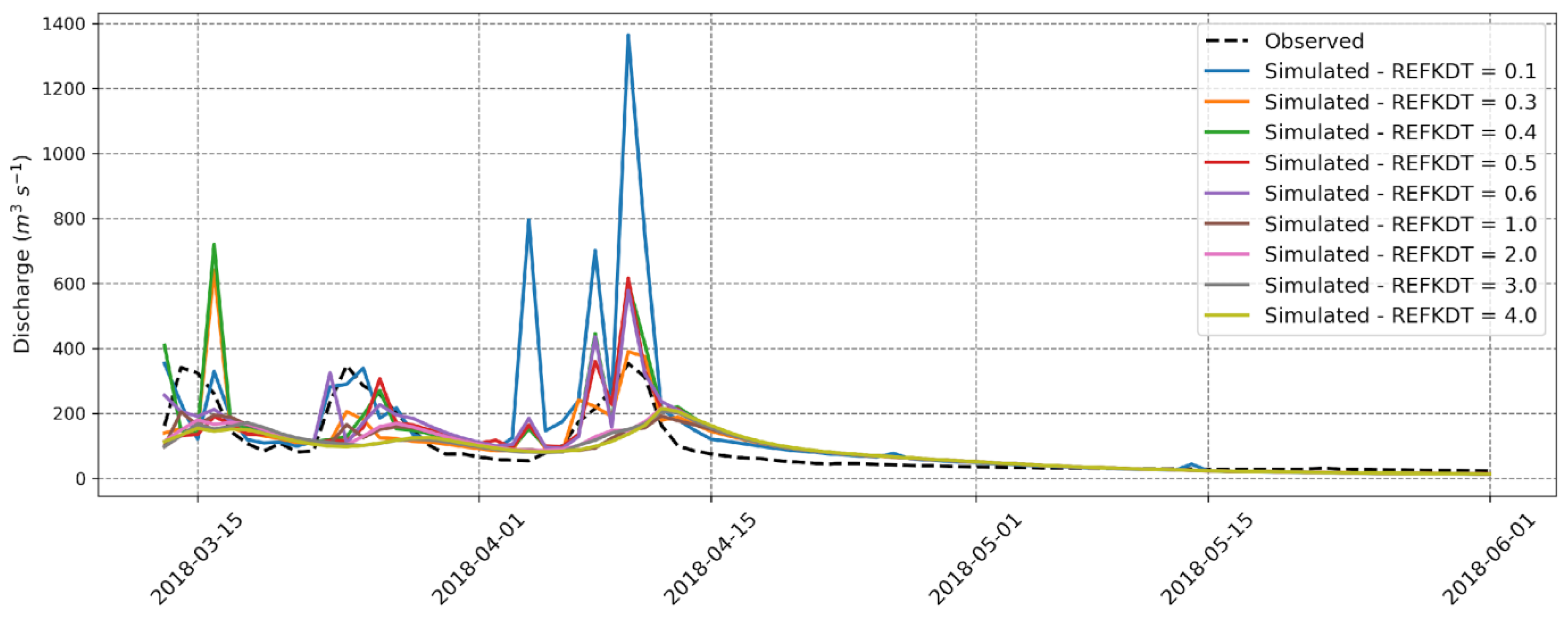
49]. Sensitivity tests were initially conducted for the Manuel Alves Pequeno River using discharge data from the Itacajá station, focusing first on the REFKDT parameter that controls the hydrograph volume. Its default value is 3, with a feasible range from 0.1 to 10 [20]. This parameter can significantly affect the simulated discharge values, depending on climatic conditions and runoff generation mechanisms in different watersheds. Even in a physics-based model like WRF-Hydro, adjusting REFKDT and the other three empirical parameters is inevitable, a result of our inability to model all processes [48]. Based on the reviewed literature in this study, the values chosen for testing were 0.1, 0.3, 0.4, 0.5, 0.6, 1, 2, 3, and 4. Figure 4 illustrates the observed and WRF-Hydro-simulated discharges at the Itacajá station location for the specified REFKDT values from 13 March to 1 June 2018.
A significant impact of the infiltration factor (REFKDT) on model discharge results is observed, highlighting the sensitivity of this parameter, as demonstrated in [19] for the case in the Ouémé River, in [20] for the Upper Tana River Basin, both in West Africa, and by [47] on the Korean Peninsula. [49] conducted a calibration process similar to that of WRF-Hydro simulations. They used various values for REFKDT, REFDK, and OVROUGHRTFAC to identify the most effective parameter values for their basin, located in western Turkey. Their findings highlighted that REFKDT is the parameter with the highest sensitivity when it comes to regulating runoff reactions during rainfall events. They also observed that higher REFKDT values lead to a reduction in discharge. In the WRF-Hydro model, the water entering the channel, affecting the discharge, is primarily derived from the amount of precipitation exceeding the infiltration capacity at each grid cell [17]. As illustrated in studies in the Mediterranean region [16] and in the Daqinghe Basin in northern China [17], it is generally observed that an increase in REFKDT results in a decrease in surface runoff and, consequently, a reduction in simulated discharge. This trend is visible in the graph for the period from 1 April to 15 April 2018, where REFKDT = 0.1 shows a peak discharge close to 1400 m3 s−1, REFKDT = 0.5, around 600 m3 s−1, and for REFKDT values of 2, 3, and 4, the peak is around 200 m3 s−1. Table 2 presents the statistical coefficients NSE, RSR, R, and PBIAS when comparing simulated and observed discharge for each REFKDT value.
This finding aligns with [54], who emphasizes the WRF-Hydro model’s capability to adeptly manage and simulate conditions of peak flows. Incorporating these advanced features of the WRF-Hydro model, our work strategically portrays a detailed and enriched understanding of flood peaks and their dynamic behaviors. Such precise modeling, supported by robust empirical evidence, amplifies the reliability of our hydrological forecasts and analyses, making them especially pertinent in navigating and managing scenarios characterized by extreme hydrological events.
The PBIAS index generally indicates a decrease in average discharge with the increase in REFKDT, representing maximum overestimation (PBIAS = 50.43) for REFKDT = 0.1 and the highest magnitude of underestimation (PBIAS = −12.56) when REFKDT = 4. The REFKDT values of 0.5, 0.6, 1, and 2 yielded similar statistical indices. REFKDT = 0.6 was selected as it exhibited the best correlation (R = 0.78), one of the highest NSE values, and the lowest error (RSR = 0.73). The results of the statistical metrics are also interesting for REFKDT = 0.3, as it showed a lower PBIAS and reasonable values for other metrics. However, we did not use this value because, during the second peak flow, around 22 March 2018, the simulated discharge showed a significant underestimation.
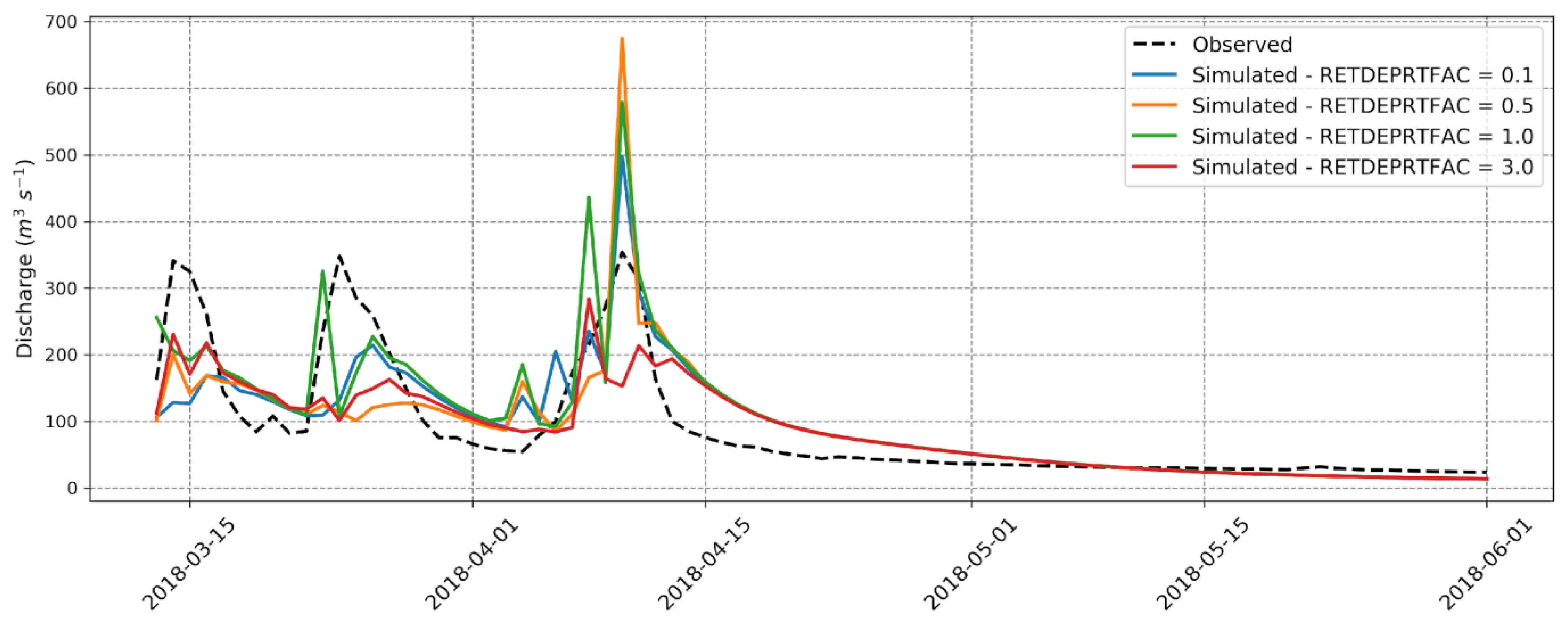
With the selection of REFKDT = 0.6, values of 0.1, 0.5, 1, and 3 were analyzed for the parameter RETDEPRTFAC. Its default value is 1, and it has a function similar to REFKDT, potentially influencing the calculation of surface runoff. This is because RETDEPRTFAC serves as a factor of maximum retention depth; before that, the flow is routed as overland flow [13]. Figure 5 presents the observed discharge values at the hydrological station and the simulated values for the mentioned RETDEPRTFAC parameters.
The values of RETDEPRTFAC 0.1, 0.5, and 1 evaluated in [17] showed virtually no influence on their discharge results. In this study, there is a slight variation in the simulated discharge at these values, specifically at peak points around 10 April 2018, suggesting that the influence of the RETDEPRTFAC parameter on channel discharge is not evident. Table 3 presents the statistical coefficients derived from the data represented in the plot.
In the WRF-Hydro modeling system, it is generally expected that surface runoff, and consequently, discharge should decrease with an increase in RETDEPRTFAC. This trend was not consistently observed except for the highest value, RETDEPRTFAC = 3, which displayed the lowest PBIAS index (−2.60), indicating the only underestimation of the simulated data relative to the observed data.
As observed in [17], or in cases in the Kaidu River Basin in China [55], in the Eastern Black Sea and Mediterranean regions [18], where discharge results showed nearly no response to RETDEPRTFAC, the statistical indices demonstrate lower variability compared to the other parameters, suggesting that RETDEPRTFAC has weaker sensitivity in simulating discharge among the parameters tested in this study. This may be due to significant variations in altitude and terrain in the study area, as suggested in [17], where little accumulation occurs on steep surfaces. Despite its limited influence, the default value, RETDEPRTFAC = 1, yielded the best correlation (R) and an NSE closest to 1. 
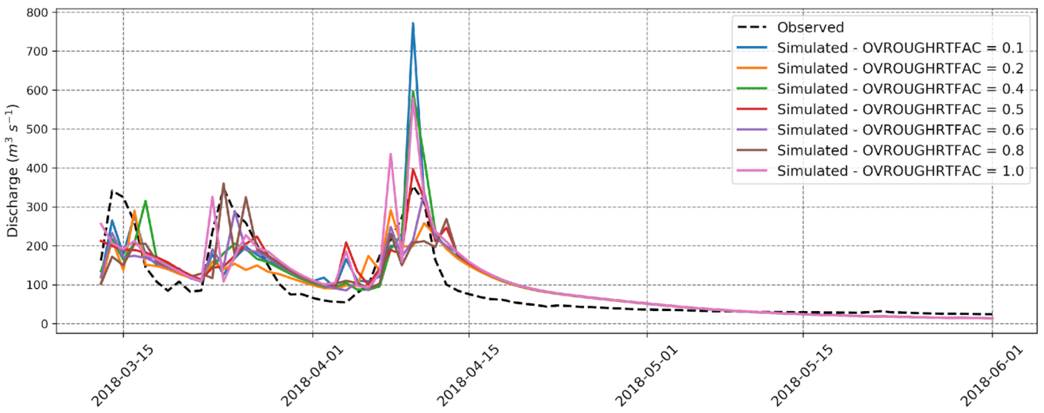
Figure 6 presents the discharge rates observed at the Itacajá station and those simulated by WRF-Hydro with sensitivity tests for OVROUGHRTFAC.
Just as in the study conducted in the Upper Trinity River Basin, located in North-Central Texas, USA [48], infiltration processes were more sensitive to REFKDT and OVROUGHRTFAC. Consequently, significantly altering the discharge data at certain OVROUGHRTFAC values changes the shape of the hydrographs in these cases, showing peak discharges at separate times and values. At the maximum point of the observed simulations, for example, around 10 April 2018, the discharge is greater when OVROUGHRTFAC is 0.1 than when this parameter is 0.5, which in turn is greater when OVROUGHRTFAC = 0.8. Table 4 shows the statistical coefficients for all parameters.
It is observed, as in [17], that this parameter had a quite significant impact on improving the statistical indices when varying OVROUGHRTFAC relative to its default value, except when OVROUGHRTFAC = 0.1. In these cases of improvement, the NSE, which is the statistical index used in all WRF-Hydro flow studies, improved by a scale of 21% to 47%. The other statistical indices also improved considerably, making it, along with REFKDT, the parameter that most influenced the flow simulation in this study.
Lastly, after analyzing the transmission of surface runoff to the river network, the transport of water along the channels was assessed through the sensitivity test of the channel roughness parameter (MannN). This transport can also affect the shape of the hydrograph. The channel geometric properties were set to their default values because there are no available channel cross-section data for the region concerning stream orders. In WRF-Hydro, channel properties such as average channel base width (Bw), initial water depth (HLINK), channel slope (Ch SSlp), and Manning’s coefficient (MannN) are introduced based on each stream order. The default values of the channel parameters are provided in Table 5.
The adjustment of the Manning coefficient is carried out by multiplying each initial MannN value by a scaling factor, thereby preserving the spatial patterns of the parameters during calibration. This scaling factor becomes the calibration parameter, generating MannN values for all the river channels. In this study, the values were established to cover a range between 0.2 and 2, including increments of 0.2 [19]. 
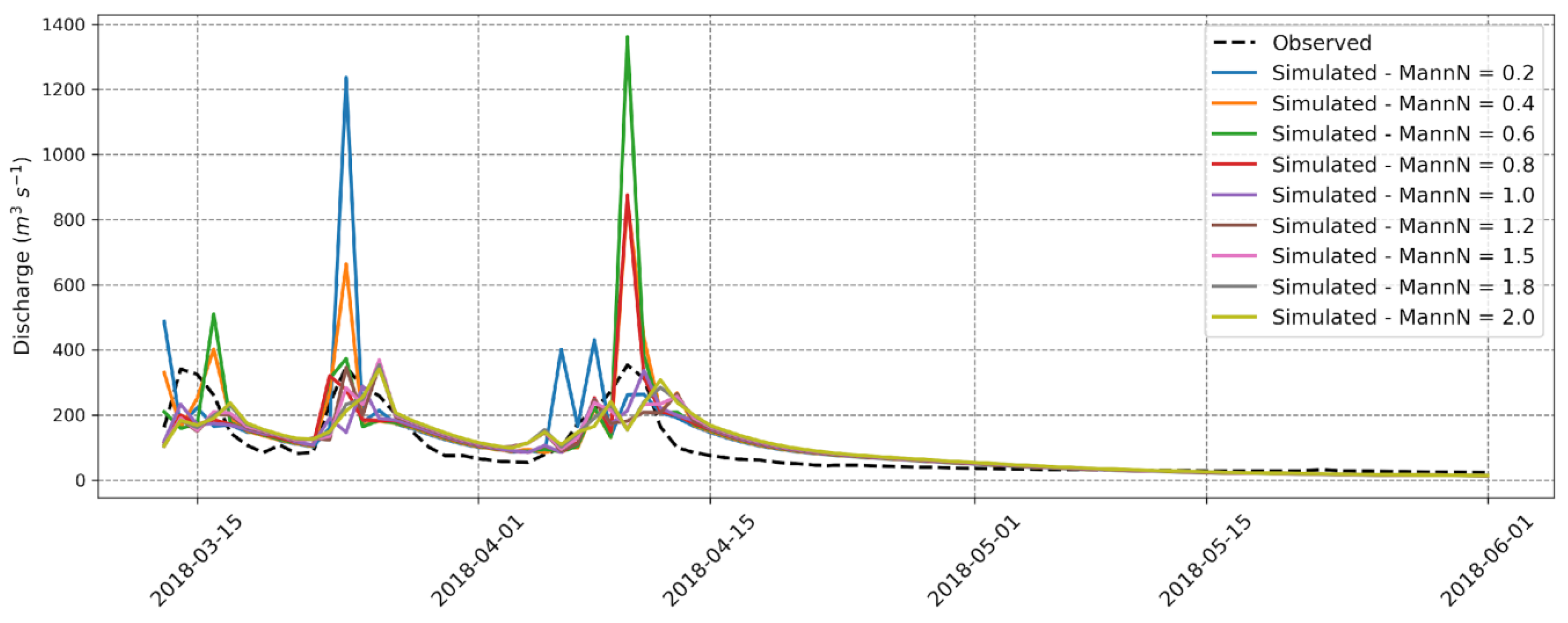
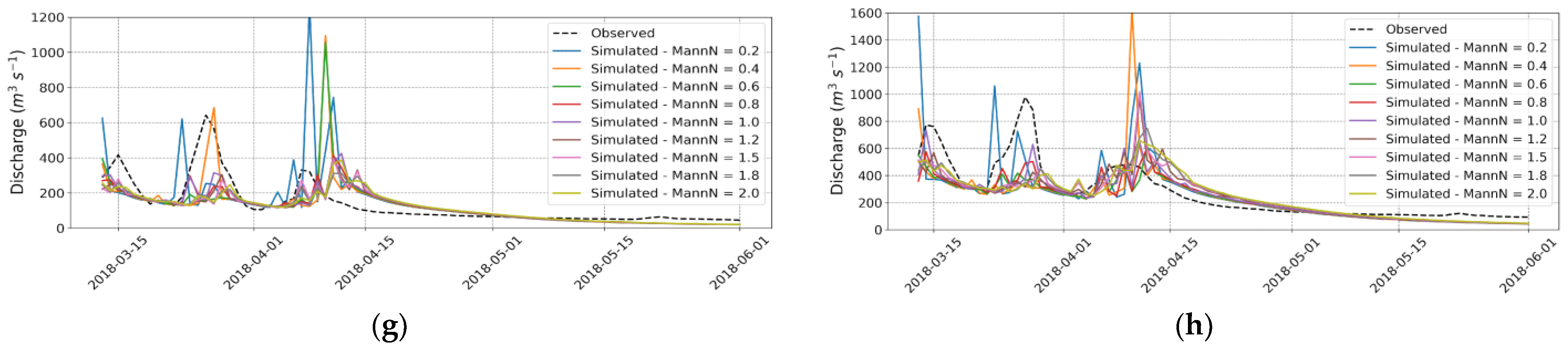
Figure 7 displays the simulated flow rates with their respective MannN parameters and the flow rate measured at the hydrological station.
When the MannN coefficients ranged from 0.2 to 0.8, the simulated flow rate peaks were significantly higher than the values obtained when MannN equals or exceeds 1. Flow rates exceeding 400 m3 s−1 were not observed within this range, indicating a stabilization of the flow rate peaks. Table 6 displays the statistical indices for each observed MannN value.
The more pronounced overestimation displayed graphically when MannN is less than 1 is corroborated by the PBIAS index, which shows higher results in these cases, reaching over 5 times the smallest value obtained when MannN is 1 (PBIAS = 4.99). All other statistical indices were better at the default value of the channel roughness parameter when MannN = 1.
Therefore, the best performance in flow rate simulation with WRF-Hydro in this study was achieved when REFKDT = 0.6, RETDEPRTFAC = 1.0, OVROUGHRTFAC = 0.6, and MannN = 1.0. The statistical indices NSE = 0.69, RSR = 0.56, R = 0.83, and PBIAS = 4.99 indicate superior results. According to [51], the range of NSE > 0.65 and RSR ≤ 0.60 is considered good for the evaluation of hydrological models, and the PBIAS index ≤ ±10% is considered exceptionally good. In their best flow rate simulation with WRF-Hydro in coupled mode, [19] obtained a correlation index R = 0.84, [44] achieved R = 0.83 and NSE = 0.7, and [20] reported NSE = 0.71 and RSR = 0.51.

3.2. Results at the Other Two Hydrological Stations

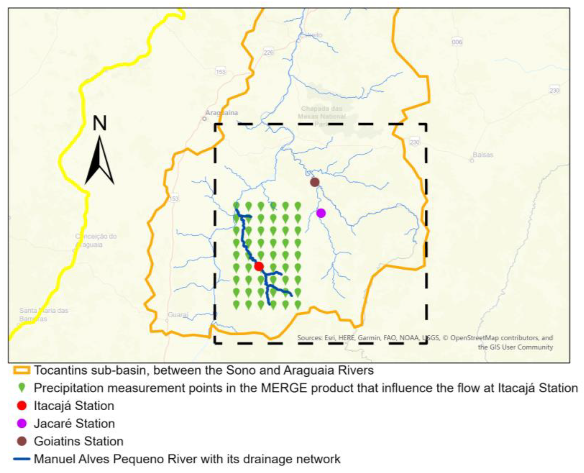
In the Jacaré and Goiatins stations, which measure the flow of the Vermelho and Manuel Alves Grande rivers, the same rain event from the Itacajá station was analyzed, covering the period from 13 March to 1 June 2018. Since it is the same simulation, the standard choice of hydrological model parameter values was maintained. Table 7 shows the statistical parameters for the results of these simulations.
Similarly, in the analysis conducted at the Itacajá station, the same values assigned to REFKDT, RETDEPRTFAC, OVROUGHRTFAC, and MannN converged to the best statistical indices in most cases of the simulations that were analyzed with the Jacaré and Goiatins stations. Furthermore, the improvement in results was more pronounced when changing the parameters REFKDT and OVROUGHRTFAC.
The statistical coefficient PBIAS is often lower as the hydrological model parameters are larger, especially for the REFKDT parameter, indicating a decrease in surface runoff and a consequent reduction in simulated flow. 
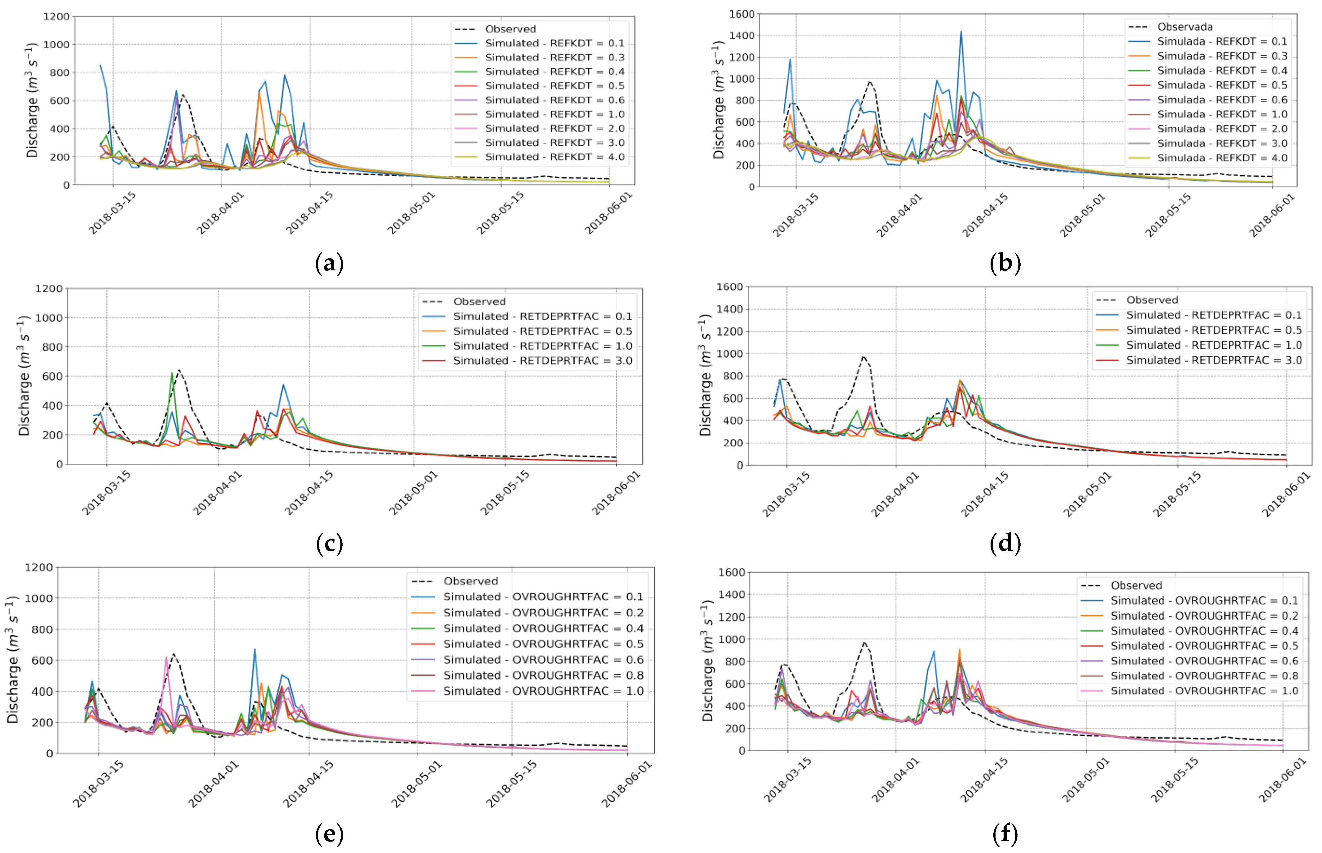
Figure 8 shows the simulations compared with the Jacaré and Goiatins stations.
Indeed, it is noticeable that lower REFKDT values exhibit higher peak points compared to higher values, which show flow results close to each other. It can be observed in the first two peaks of the observed flow. The simulations, in the majority of cases, have their values underestimated. However, at the last peak, the simulated flows are overestimated.
Despite the three stations belonging to the same watershed and the same simulation tests being carried out, it is evident that the statistical indices of the simulations compared to the Jacaré and Goiatins stations are lower than those of the simulation conducted with the Itacajá station. This could be related to an increased disparity in the distribution of rainfall in both spatial and temporal dimensions, which worsens the WRF-Hydro simulations. This could result from errors in the directional data, in this case, the GDAS-FNL data used in the WRF, which indirectly affects the WRF-Hydro’s performance in flow simulation [17].

3.3. Error in Simulated Precipitation

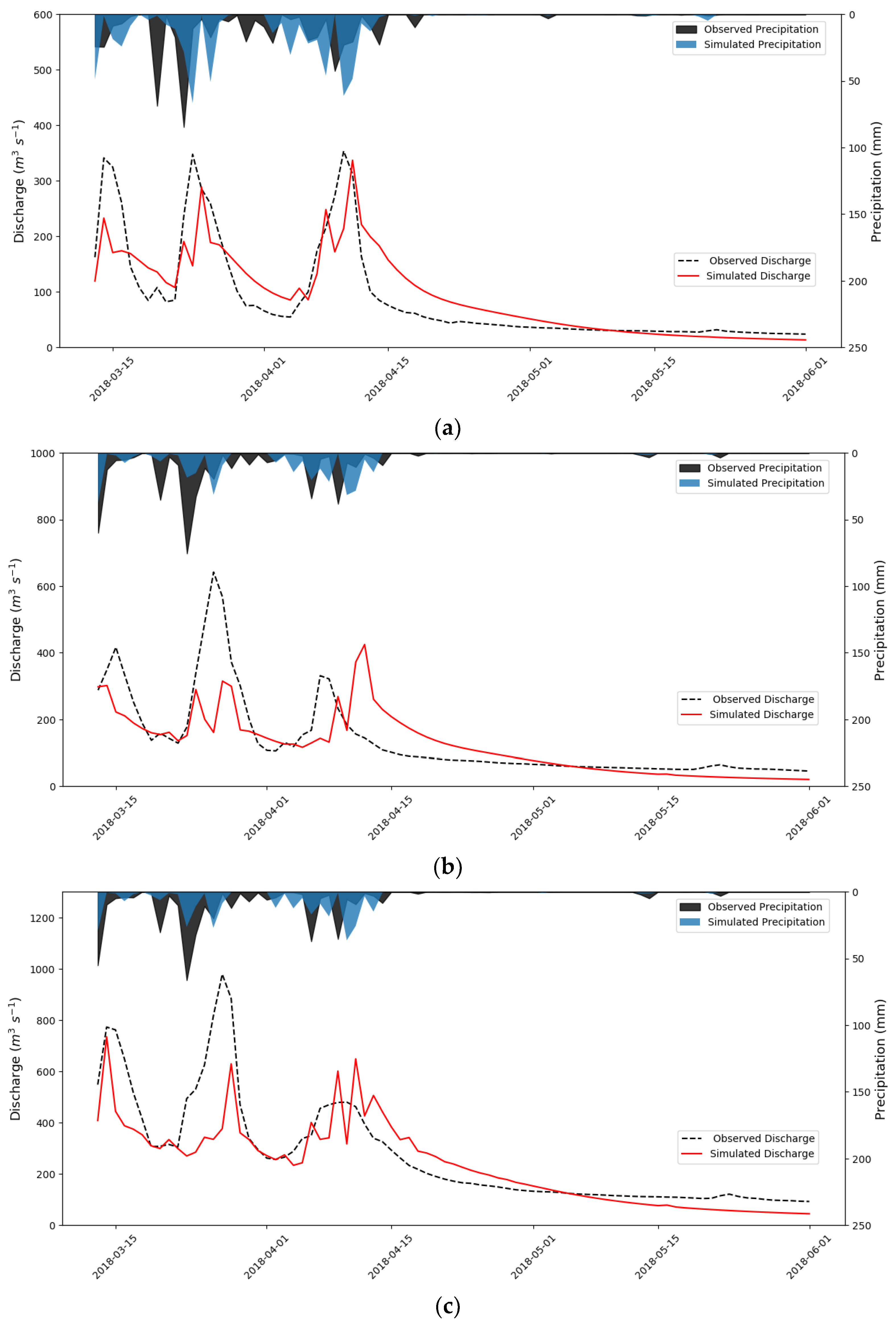
The values of simulated precipitation, when compared to the values of measured precipitation using the MERGE product in the drainage network region of the Rio Manuel Alves Pequeno (where the Itacajá station is located), exhibit a more uniform distribution of rainfall over time than in the drainage network regions of the Rio Manuel Alves Grande and Vermelho (where the Goiatins and Jacaré stations are located, respectively). This directly affects the difference between the peaks of simulated and observed flows and the timing at which they occur.
Figure 9 displays the daily averages of precipitation obtained from the MERGE product within the drainage network area of each river, as well as those simulated by the WRF within the same area. It also shows the observed flows at river gauge stations and simulated flows in the WRF-Hydro model under the best-performing conditions, characterized by REFKDT = 0.6, RETDEPRTFAC = 1.0, OVROUGHRTFAC = 0.6, and MannN = 1.0.
It can be observed that the simulated precipitation in the observed data presented in Figure 9b,c is underestimated, while Figure 9a exhibits a seemingly smaller overestimation. It is also noteworthy that the inherent uncertainty in climate predictions resulting from the WRF simulation, conducted with GDAS-FNL input data, has impacted the results of the WRF-Hydro simulation. Table 8 displays the relative errors of accumulated simulated and observed rainfall events within the drainage networks of the three analyzed rivers.
Indeed, the drainage network area of the Rio Manuel Alves Pequeno demonstrates the best results in precipitation simulation among the other two areas, with the smallest absolute value of ER = 10.66%. Conversely, the WRF model exhibits the poorest performance in simulating rainfall accumulation for the Rio Vermelho, with the highest relative error. This discrepancy could potentially impact the results of flow simulation in WRF-Hydro. Therefore, it is essential to emphasize that the calibration of WRF-Hydro parameters in this study cannot eliminate the errors in rainfall simulation originating from input data, directly influencing flow results. However, even with errors stemming from precipitation and considering the possibility of improving data through further study of WRF-Hydro in Brazilian regions, the strong correlation observed between simulated and observed flows when modifying hydrological parameters can serve as a starting point for using this hydrometeorological model in future research related to water resources management in Brazil.

3.4. Implications for Water Resources Management

Our study contributes valuable insights into the hydrological dynamics of the Manuel Alves Pequeno, Vermelho, and Manuel Alves Grande rivers, providing a foundation for improved water resources management practices in the MATOPIBA region. The accurate representation of hydrological parameters, such as soil infiltration, surface retention depth, and land surface roughness, is critical for making informed decisions regarding water allocation, especially in areas experiencing climate change and rapid urban and agricultural expansions.
Water resource management is a crucial aspect of ensuring sustainable water allocation, addressing the challenges posed by climate change, and expanding urban and agricultural areas. Accurate representation of hydrological parameters by numerical models such as WRF-Hydro is essential for making informed decisions regarding water resources [13]. By accurately simulating streamflow, the research serves as a benchmark for future hydrological modeling efforts in the MATOPIBA region, guiding water resource management strategies to meet the demands of a changing climate and evolving land use patterns. The efficient simulation of streamflow is a prerequisite for any effective water management plan. For example, [56] assessed a water security threat index for the western region of Bahia, an area within the MATOPIBA region and one of Brazil’s primary areas for agricultural exploitation. The authors estimated that 66% of agricultural enterprises effectively manage the water resources in the region. However, their results suggest that threats to water availability in the region will significantly increase by 2040.
Environmental exploitation, stemming from Brazil’s international significance as a food exporter, climate change, land use/land cover (LULC) changes, and desertification processes are key factors exacerbating this issue. LULC and climate change can significantly affect surface runoff, which is a key component of water resource management. Models that investigate the changes in hydrological pathways caused by climate and human activities can provide valuable frameworks for understanding and managing surface runoff [57,58]. Analyzing the impact of climate change on net irrigation water demand can help assess the future water resources in areas equipped for irrigation [59]. Therefore, considering the use of modern hydrometeorological models like WRF-Hydro can assist decision-makers, whether in the public or private sectors, in better managing the available water resources.
Climate change significantly impacts water resources and agriculture, highlighting the crucial need to understand how climate shifts interact with human activities in assessing water availability and food production [60]. In the bigger picture, global climate change poses threats to farming by messing with natural resources, especially rainfall patterns. Extreme downpours linked to climate change boost rainfall erosivity, causing more soil erosion. On the other hand, less rain creates water shortages for farming. Realizing how vital it is to model climate conditions under global change, particularly where rainfall data are on the rise, a study focusing on the MATOPIBA region becomes a big deal.
Ref. [61] projected rainfall erosivity in the Tocantins-Araguaia River basin for the 21st century under IPCC AR5 scenarios (RCP4.5 and RCP8.5). Using downscaling from four CMIP5 global climate models via the Eta regional climate model, the study showed a drop in erosivity for both scenarios due to less rainfall. But, even with this drop, the erosivity values are still significant, shouting out the need for robust soil conservation practices. Plus, the lower rainfall hints at less water for long-cycle crops and more uneven and less intense rainfall. In this complicated mix of climate challenges, our results with WRF-Hydro rainfall and streamflow simulation in the MATOPIBA region stand out, giving vital insights for managing water resources and planning agriculture to mitigate future scarcity.
Coupled hydrologic models, such as WRF-Hydro, are valuable tools for estimating water balance, analyzing groundwater levels and surface water discharges, and extrapolating to different scenarios and large basins [62,63]. In hydrological studies, the availability of data is vital. Data on rainfall, runoff, and other hydrological parameters are essential for accurate modeling and understanding of the dynamics of river basins [64]. These models can provide detailed information for water resource management and help analyze the impacts of meteorological and LULC changes.
Additionally, our research serves as a benchmark for future hydrological modeling efforts in the MATOPIBA region, guiding water resources management strategies to meet the demands of a changing climate and evolving land use patterns. While the manuscript may not explicitly delve into the policy and management aspects, the accurate simulation of streamflow is a prerequisite for any effective water management plan.

4. Summary and Conclusions

This study investigated the simulation of streamflow from 13 March to 1 June 2018, using the WRF-Hydro model in three rivers within the Tocantins/Araguaia sub-basin, between the Sono and Araguaia rivers in the MATOPIBA region. The analysis focused on assessing the influence of hydrological parameters, including the infiltration factor (REFKDT), surface retention depth (RETDEPRT), surface roughness (OVROUGHRT), and channel roughness (MannN). Sensitivity tests of these parameters were conducted concerning discharge data from the Itacajá station, located on the Manuel Alves Pequeno River. The parameter values selected for the Jacaré and Goiatins stations, which measure the flow of the Vermelho and Manuel Alves Grande rivers, respectively, followed the same pattern.
The study found that REFKDT and OVROUGHRTFAC were the parameters that had the most significant impact on the statistical indices obtained from the comparison between observed and simulated discharge. In many cases, the statistical coefficient PBIAS was lower when the model hydrological parameters were larger, particularly in the case of the REFKDT parameter. This suggests a decrease in surface runoff and a consequent reduction in simulated discharge.
The best discharge simulation performance was achieved when REFKDT = 0.6, RETDEPRTFAC = 1.0, OVROUGHRTFAC = 0.6, and MannN = 1.0. The highest statistical indices obtained were NSE = 0.69, RSR = 0.56, R = 0.83, and PBIAS = 4.99 in the simulation compared to observations at the Itacajá station. At the Jacaré station location, the statistical indices for discharge simulation were lower due to the less uniform temporal distribution of rainfall compared to the regions within the drainage network of the other two hydrometric stations.
These results indicate that the fully coupled WRF-Hydro modeling system demonstrates a good tendency in river discharge simulation, highlighting the considerable influence of model hydrological parameters and temporal rainfall distribution at each observation location. Future works involve improving results by analyzing additional model variables and incorporating other resources, such as artificial intelligence. Similar parameterizations will also be applied to different periods of intense rainfall in this region, aiming to effectively assess water resources in MATOPIBA basins and other Brazilian regions.

Author Contributions

Conceptualization, D.G.S. and J.R.D.d.S.J.; methodology, D.N.d.S.R. and A.R.S.; software, D.G.S., J.R.D.d.S.J. and F.M.d.S.; validation, D.G.S., J.R.D.d.S.J. and F.M.d.S.; formal analysis, T.S.d.S.; investigation, D.G.S.; resources, J.R.D.d.S.J.; data curation, D.G.S.; writing—original draft preparation, D.G.S. and J.R.D.d.S.J.; writing—review and editing, D.N.d.S.R., A.R.S. and T.S.d.S.; supervision, D.M.M. All authors have read and agreed to the published version of the manuscript.

Funding

This research received no external funding.

Data Availability Statement

Data available upon request.

Conflicts of Interest

The authors declare no conflict of interest.

References

  1. Farjalla, V.F.; Pires, A.P.F.; Agostinho, A.A.; Amado, A.M.; Bozelli, R.L.; Dias, B.F.S.; Dib, V.; Faria, B.M.; Figueiredo, A.; Gomes, E.A.T.; et al. Turning water abundance into sustainability in Brazil. Front. Environ. 2021, 9, 727051. [Google Scholar] [CrossRef]
  2. ANA—Agência Nacional de Águas e Saneamento Básico. Conjuntura dos Recursos Hídricos no Brasil 2019: Informe Anual; Agência Nacional de Águas: Brasília, Brazil, 2019. Available online: http://www.snirh.gov.br/portal/snirh/centrais-de-conteudos/conjuntura-dos-recursos-hidricos/conjuntura_informe_anual_2019-versao_web-0212-1.pdf (accessed on 16 September 2023).
  3. EMBRAPA. Empresa Brasileira de Pesquisa e Agropecuária. Available online: https://www.embrapa.br/documents/10180/26187851/O+agro+no+Brasil+e+no+mundo/098fc6c1-a4b4-7150-fad7-aaa026c94a40#:~:text=O%20Brasil%20atingiu%20o%20posto,3%20trilh%C3%B5es%20de%20d%C3%B3lares%20americanos (accessed on 15 September 2023).
  4. Silva, P.R.; Vianna, J.N.S. A Região de MATOPIBA (Brasil) e o Nexus Água-Energia-Alimentos. Desenvolv. E Meio Ambiente 2022, 59, 338–353. [Google Scholar] [CrossRef]
  5. ANA—Agência Nacional de Águas. Conjuntura dos Recursos Hídricos No Brasil: Regiões Hidrográficas Brasileiras—Edição Especial; Agência Nacional de Águas: Brasília, Brazil, 2015. Available online: http://www.snirh.gov.br/portal/snirh/centrais-de-conteudos/conjuntura-dos-recursos-hidricos/regioeshidrograficas2014.pdf (accessed on 15 September 2023).
  6. Gomes, D.J.C.; Ferreira, N.S.; Lima, A.M.M. Tendências de variabilidade espaço-temporal pluviométrica nabacia hidrográfica do Rio Araguaia. Enciclopédia Biosf. 2019, 16, 1421–1433. Available online: https://conhecer.org.br/ojs/index.php/biosfera/article/view/292 (accessed on 16 September 2023). [CrossRef]
  7. Morais, J.L.M.; Fadul Élvia Cerqueira, L.S. Limites e desafios na gestão de recursos hídricos por comitês de bacias hidrográficas: Um estudo nos estados do nordeste do Brasil. Rev. Eletrônica Adm. 2018, 24, 238–264. [Google Scholar] [CrossRef]
  8. Siad, S.M.; Iacobellis, V.; Zdruli, P.; Gioia, A.; Stavi, I.; Hoogenboom, G. A review of coupled hydrologic and crop growth models. Agric. Water Manag. 2019, 224, 105746. [Google Scholar] [CrossRef]
  9. Cunha, Z.A.; Mello, C.R.; Beskow, S.; Vargas, M.M.; Guzman, J.A.; Moura, M.M. A Modeling Approach for Analyzing the Hydrological Impacts of the Agribusiness Land-Use Scenarios in an Amazon Basin. Land 2023, 12, 1422. [Google Scholar] [CrossRef]
  10. Fontes, V.C. Efeitos da Expansão Agrícola na Disponibilidade Hídrica Do oeste da Bahia via Modelagem Hidrológica. Ph.D. Thesis, Universidade Federal de Viçosa, Viçosa, Brazil, 2022. [Google Scholar] [CrossRef]
  11. Powers, J.G.; Klemp, J.B.; Skamarock, W.C.; Davis, C.A.; Dudhia, J.; Gill, D.O.; Coen, J.L.; Gochis, D.J.; Ahmadov, R.; Peckham, S.E.; et al. The Weather Research and Forecasting Model: Overview, System Efforts, and Future Directions. Bull. Am. Meteorol. Soc. 2017, 98, 1717–1737. [Google Scholar] [CrossRef]
  12. Naabil, E.; Kouadio, K.; Lamptey, B.; Annor, T.; Chukwudi Achugbu, I. Tono basin climate modeling, the potential advantage of fully coupled WRF/WRF-Hydro modeling System. Model. Earth Syst. Environ. 2023, 9, 1669–1679. [Google Scholar] [CrossRef]
  13. Gochis, D.J.M.; Barlage, R.; Cabell, M.; Casali, A.; Dugger, K.; FitzGerald, M.; McAllister, J.; McCreight, A.; RafieeiNasab, L.; Read, K.; et al. The WRF-Hydro Modeling System Technical Description, (Version 5.1.1). NCAR Technical Note. 107 Pages. 2020. Available online: https://ral.ucar.edu/projects/wrf_hydro/documentation/wrf-hydro-v511-documentation (accessed on 10 July 2023).
  14. Sun, M.; Li, Z.; Yao, C.; Liu, Z.; Wang, J.; Hou, A.; Zhang, K.; Huo, W.; Liu, M. Evaluation of Flood Prediction Capability of the WRF-Hydro Model Based on Multiple Forcing Scenarios. Water 2020, 12, 874. [Google Scholar] [CrossRef]
  15. Cho, K.; Kim, Y. Improving dis prediction in the WRF-Hydro model with LSTM networks. J. Hydrol. 2022, 605, 127297. [Google Scholar] [CrossRef]
  16. Givati, A.; Gochis, D.; Rummler, T.; Kunstmann, H. Comparing One-Way and Two-Way Coupled Hydrometeorological Forecasting Systems for Flood Forecasting in the Mediterranean Region. Hydrology 2016, 3, 19. [Google Scholar] [CrossRef]
  17. Liu, Y.; Liu, J.; Li, C.; Yu, F.; Wang, W.; Qiu, Q. Parameter Sensitivity Analysis of the WRF-Hydro Modeling System for Streamflow Simulation: A Case Study in Semi-Humid and Semi-Arid Catchments of Northern China. Asia Pac. J. Atmos. Sci. 2021, 57, 451–466. [Google Scholar] [CrossRef]
  18. Kilicarslan, B.M.; Yucel, I.; Pilatin, H.; Duzenli, E.; Yilmaz, M.T. Improving WRF-Hydro runoff simulations of heavy floods through the sea surface temperature fields with higher spatio-temporal resolution. Hydrol. Process. 2021, 35, e14338. [Google Scholar] [CrossRef]
  19. Quenum, G.M.L.D.; Arnault, J.; Klutse, N.A.B.; Zhang, Z.; Kunstmann, H.; Oguntunde, P.G. Potential of the coupled WRF/WRF-hydro modeling system for flood forecasting in the Ouémé River (West Africa). Water 2022, 14, 1192. [Google Scholar] [CrossRef]
  20. Kerandi, N.; Arnault, J.; Laux, P.; Wagner, S.; Kitheka, J.; Kunstmann, H. Joint atmospheric-terrestrial water balances for East Africa: A WRF-Hydro case study for the upper Tana River basin. Theor. Appl. Climatol. 2017, 131, 1337–1355. [Google Scholar] [CrossRef]
  21. Magalhães, L.A.; Miranda, E.E. MATOPIBA: Quadro Natural; EMBRAPA: Campinas, Brazil, 2014; Available online: https://ainfo.cnptia.embrapa.br/digital/bitstream/item/139255/1/NT5-Matopiba-Quadro-Natural.pdf (accessed on 17 September 2023).
  22. Reis, L.C.; Silva, C.M.; Bezerra, B.G.; Spyrides, M.H.C. Caracterização da variabilidade da precipitação no MATOPIBA, região produtora de soja. Rev. Bras. De Geogr. Física 2020, 13, 1425–1441. [Google Scholar] [CrossRef]
  23. De Cristo, S.S.V.; Robaina, L.E.S. Caracterização da Rede Hidrográfica na Estação Ecológica Serra Geral do Tocantins, Estados do Tocantins e Bahia. Geogr. Ensino Pesqui. 2014, 18, 103–116. [Google Scholar] [CrossRef]
  24. Mauriz, T.V.M. Análise Do Inventário Hidroelétrico da Bacia do rio do sono—TO, Subsídio Para a Identificação de Variáveis Socioambientais Aplicadas na Construção de um Modelo de Inventário Hidroelétrico Dinâmico. Master’s Thesis, Universidade Católica de Brasília, Brasília, Brazil, 2008. Available online: https://bdtd.ucb.br:8443/jspui/handle/123456789/1748 (accessed on 17 September 2023).
  25. ANA. Agência Nacional de Águas e Saneamento Básico. Available online: www.snirh.gov.br (accessed on 15 September 2023).
  26. Rozante, J.R.; Moreira, D.S.; Gonçalves, L.G.G.; Vila, D.A. Combining TRMM and Surface Observations of Precipitation: Technique and Validation Over South America. Weather Forecast. 2010, 25, 885–894. [Google Scholar] [CrossRef]
  27. Rozante, J.R.; Gutierrez, E.R.; Fernandes, A.D.A.; Vila, D.A. Performance of precipitation products obtained from combinations of satellite and surface observations. Int. J. Remote Sens. 2020, 41, 7585–7604. [Google Scholar] [CrossRef]
  28. INPE. Instituto Nacional de Pesquisas Espaciais. Available online: http://ftp.cptec.inpe.br/modelos/tempo/MERGE/GPM/DAILY/ (accessed on 15 September 2023).
  29. NCEP, National Centers for Environmental Prediction/National Weather Service/NOAA/U.S. Department of Commerce. NCEP GDAS/FNL 0.25 Degree Global Tropospheric Analyses and Forecast Grids. Research Data Archive at the National Center for Atmospheric Research, Computational and Information Systems Laboratory. 2015. Available online: https://rda.ucar.edu/datasets/ds083.3/ (accessed on 1 May 2023).
  30. Pedruzzi, R.; Andreão, W.L.; Baek, B.H.; Hudke, A.P.; Glotfelty, T.W.; Freitas, E.D.D.; Martins, J.; Bowden, J.H.; Pinto, J.A.; Alonso, M.F.; et al. Update of land use/land cover and soil texture for Brazil: Impact on WRF modeling results over São Paulo. Atmos. Environ. 2022, 268, 118760. [Google Scholar] [CrossRef]
  31. Bae, S.Y.; Hong, S.Y.; Lim, K.S.S. Coupling WRF Double-Moment 6-Class Microphysics Schemes to RRTMG Radiation Scheme in Weather Research Forecasting Model. Adv. Meteorol. 2016, 2016, 5070154. [Google Scholar] [CrossRef]
  32. Stergiou, I.; Tagaris, E.; Sotiropoulou, R.E.P. Sensitivity Assessment of WRF Parameterizations over Europe. Proceedings 2017, 1, 119. [Google Scholar] [CrossRef]
  33. Sousa, J.M.D.; Candido, L.A.; Silva, J.T.D.; Andreoli, R.V.; Kayano, M.T.; Manzi, A.O.; Souza, R.A.F.; Souza, E.B.; Vieira, S.O. Avaliação da Habilidade do Modelo WRF em Representar a Precipitação na Amazônia Usando Diferentes Escalas. Rev. Bras. Meteorol. 2019, 34, 255–273. [Google Scholar] [CrossRef]
  34. Wang, X.; Tolksdorf, V.; Otto, M.; Scherer, D. WRF-based Dynamical Downscaling of ERA5 Reanalysis Data for High Mountain Asia: Towards a New Version of the High Asia Refined Analysis. Int. J. Climatol. 2020, 41, 743–762. [Google Scholar] [CrossRef]
  35. Hong, S.Y.; Lim, J.O.J. The WRF single–moment 6–class microphysics scheme (WSM6). Asia Pac. J. Atmos. Sci. 2006, 42, 129–151. Available online: https://api.semanticscholar.org/CorpusID:120362377 (accessed on 16 July 2022).
  36. Grell, G.A. Prognostic evaluation of assumptions used by cumulus parameterizations. Mon. Weather Rev. 1993, 121, 764–787. [Google Scholar] [CrossRef]
  37. Iacono, M.J.; Delamere, J.S.; Mlawer, E.J.; Shephard, M.W.; Clough, S.A.; Collins, W.D. Radiative forcing by long-lived greenhouse gases: Calculations with the AER radiative transfer models. J. Geophys. Res. Atmos. 2008, 113, D13103. [Google Scholar] [CrossRef]
  38. Nakanishi, M.; Niino, H. An improved Mellor–Yamada level-3 model: Its numerical stability and application to a regional prediction of advection fog. Bound.-Layer Meteorol. 2006, 119, 397–407. [Google Scholar] [CrossRef]
  39. Tewari, M.; Chen, F.; Wang, W.; Dudhia, J.; Lemone, M.A.; Mitchell, K.E.; Ek, M.; Gayno, G.; Wegiel, J.W.; Cuenca, R.H. Implementation and verification of the unified NOAH land surface model in the WRF model. In Proceedings of the 20th Conference on Weather Analysis and Forecasting/16th Conference on Numerical Weather Prediction, Seattle, WA, USA, 12–16 January 2004; Available online: http://n2t.net/ark:/85065/d7fb523p (accessed on 12 March 2022).
  40. Sampson, K.; Gochis, D. WRF Hydro GIS Pre-Processing Tools, Version 5.0, Documentation. Boulder, CO: National Center for Atmospheric Research, Research Applications Laboratory. 2018. Available online: https://ral.ucar.edu/sites/default/files/public/WRFHydro_GIS_Preprocessor_v5.pdf (accessed on 10 July 2023).
  41. Manabe, S. Climate and the ocean circulation: I. The atmospheric circulation and the hydrology of the earth’s surface. Mon. Weather. Rev. 1969, 97, 739–774. [Google Scholar] [CrossRef]
  42. Milly, P.C.D. Climate, interseasonal storage of soil water, and the annual water balance. Adv. Water Resour. 1994, 17, 19–24. [Google Scholar] [CrossRef]
  43. Milly, P.C.D. Climate, soil water storage, and the average annual water balance. Water Resour. Res. 1994, 30, 2143–2156. [Google Scholar] [CrossRef]
  44. Naabil, E.; Lamptey, B.L.; Arnault, J.; Olufayo, A.; Kunstmann, H. Water resources management using the WRF-Hydro modeling system: Case-study of the Tono dam in West Africa. J. Hydrol. Reg. Stud. 2017, 12, 196–209. [Google Scholar] [CrossRef]
  45. Gochis, D.J.; Chen, F. Hydrological Enhancements to the Community Noah Land Surface Model. In NCAR Scientific Technical Report; TN-454+STR; University Corporation for Atmospheric Research: Boulder, CO, USA, 2003; 77p. [Google Scholar] [CrossRef]
  46. Wang, W.; Liu, J.; Li, C.; Liu, Y.; Yu, F. Data Assimilation for Rainfall-Runoff Prediction Based on Coupled Atmospheric-Hydrologic Systems with Variable Complexity. Remote Sens. 2021, 13, 595. [Google Scholar] [CrossRef]
  47. Ryu, Y.; Lim, Y.J.; Ji, H.S.; Park, H.H.; Chang, E.C.; Kim, B.J. Applying a coupled hydrometeorological simulation system to flash flood forecasting over the Korean Peninsula. Asia Pac. J. Atmos. Sci. 2017, 53, 421–430. [Google Scholar] [CrossRef]
  48. Zhang, J.; Lin, P.; Gao, S.; Fang, Z. Understanding the re-infiltration process to simulating streamflow in North Central Texas using the WRF-hydro modeling system. J. Hydrol. 2020, 587, 124902. [Google Scholar] [CrossRef]
  49. Yucel, I.; Onen, A.; Yilmaz, K.K.; Gochis, D.J. Calibration and evaluation of a flood forecasting system: Utility of numerical weather prediction model, data assimilation and satellite-based rainfall. J. Hydrol. 2015, 523, 49–66. [Google Scholar] [CrossRef]
  50. Zhang, Y.; Bocquet, M.; Mallet, V.; Seigneur, C.; Baklanov, A. Real-time air quality forecasting, part I: History, techniques, and current status. Atmos. Environ. 2012, 60, 632–655. [Google Scholar] [CrossRef]
  51. Liu, S.; Wang, J.; Wei, J.; Wang, H. Hydrological simulation evaluation with WRF-Hydro in a large and highly complicated watershed: The Xijiang River basin. J. Hydrol. Reg. Stud. 2021, 38, 100943. [Google Scholar] [CrossRef]
  52. Moriasi, D.N.; Arnold, J.G.; Van Liew, M.W.; Bingner, R.L.; Harmel, R.D.; Veith, T.L. Model evaluation guidelines for systematic quantification of accuracy in watershed simulations. Trans. ASABE 2007, 50, 885–900. [Google Scholar] [CrossRef]
  53. Yang, T.; Sun, F.; Gentine, P.; Liu, W.; Wang, H.; Yin, J.; Du, M.; Liu, C. Evaluation and machine learning improvement of global hydrological model-based flood simulations. Environ. Res. Lett. 2019, 14, 114027. [Google Scholar] [CrossRef]
  54. Wang, W.; Liu, J.; Xu, B.; Li, C.; Liu, Y.; Yu, F. A WRF/WRF-Hydro coupling system with an improved structure for rainfall-runoff simulation with mixed runoff generation mechanism. J. Hydrol. 2022, 612, 128049. [Google Scholar] [CrossRef]
  55. Yu, E.; Liu, X.; Li, J.; Tao, H. Calibration and Evaluation of the WRF-Hydro Model in Simulating the Streamflow over the Arid Regions of Northwest China: A Case Study in Kaidu River Basin. Sustainability 2023, 15, 6175. [Google Scholar] [CrossRef]
  56. Teixeira, A.L.D.F.; Bhaduri, A.; Siefert, C.A.C.; Iftekhar, M.S.; Bunn, S.E.; Souza, S.A.; Gonçalves, M.V.C.; Costa, L.C. Water security threats and solutions in the Grande River basin–One of the Brazilian agricultural frontiers. Sci. Total Environ. 2023, 906, 167351. [Google Scholar] [CrossRef] [PubMed]
  57. Yin, J.; He, F.; Xiong, Y.; Qiu, G. Effects of land use/land cover and climate changes on surface runoff in a semi-humid and semi-arid transition zone in northwest china. Hydrol. Earth Syst. Sci. 2017, 21, 183–196. [Google Scholar] [CrossRef]
  58. Gosling, S.; Arnell, N. A global assessment of the impact of climate change on water scarcity. Clim. Chang. 2013, 134, 371–385. [Google Scholar] [CrossRef]
  59. Alcamo, J.; Flörke, M.; Märker, M. Future long-term changes in global water resources driven by socio-economic and climatic changes. Hydrol. Sci. J. 2007, 52, 247–275. [Google Scholar] [CrossRef]
  60. Piao, S.; Ciais, P.; Huang, Y.; Shen, Z.; Peng, S.; Li, J.; Fang, J. The impacts of climate change on water resources and agriculture in China. Nature 2010, 467, 43–51. [Google Scholar] [CrossRef]
  61. Santos, W.P.; Avanzi, J.C.; Viola, M.R.; Chou, S.C.; Acuña-Guzman, S.F.; Pontes, L.M.; Curi, N. Projections of rainfall erosivity in climate change scenarios for the largest watershed within Brazilian territory. Catena 2022, 213, 106225. [Google Scholar] [CrossRef]
  62. Waseem, M.; Kachholz, F.; Klehr, W.; Tränckner, J. Suitability of a coupled hydrologic and hydraulic model to simulate surface water and groundwater hydrology in a typical north-eastern germany lowland catchment. Appl. Sci. 2020, 10, 1281. [Google Scholar] [CrossRef]
  63. Jia, Y.; Wang, H.; Zhou, Z.; Qiu, Y.; Luo, X.; Wang, J.; Du, Q. Development of the wep-l distributed hydrological model and dynamic assessment of water resources in the yellow river basin. J. Hydrol. 2006, 331, 606–629. [Google Scholar] [CrossRef]
  64. Thapa, B.; Danegulu, A.; Suwal, N.; Upadhyay, S.; Manandhar, B.; Prajapati, R. Rainfall-runoff modelling of the west rapti basin, nepal. Tech. J. 2020, 2, 99–107. [Google Scholar] [CrossRef]
Figure 1. MATOPIBA region and Tocantins sub-basin, between the Sono and Araguaia rivers.
Water 15 03902 g001
Figure 2. Grid points of the MERGE Product in the drainage network of the Manuel Alves Pequeno river.
Water 15 03902 g002
Figure 3. Flowchart of data used in the model, along with their interactions and observational data.
Water 15 03902 g003
Figure 4. Observed and simulated discharges at Itacajá station with REFKDT sensitivity tests.
Water 15 03902 g004
Figure 5. Observed discharge at the Itacajá station and simulated discharge by WRF-Hydro with sensitivity tests for RETDEPRTFAC.
Water 15 03902 g005
Figure 6. Discharge rates observed at the Itacajá station and those simulated by WRF-Hydro with sensitivity tests for OVROUGHRTFAC.
Water 15 03902 g006
Figure 7. Observed flow rates at the Itacajá station and those simulated by WRF-Hydro with sensitivity tests for MannN.
Water 15 03902 g007
Figure 8. Observed and WRF-Hydro-simulated flows at the Jacaré and Goiatins stations. (a) Jacaré station—REFKDT, (b) Goiatins station—REFKDT, (c) Jacaré station—RETDEPRTFAC, (d) Goiatins station—RETDEPRTFAC, (e) Jacaré station—OVROUGHRTFAC, (f) Goiatins station—OVROUGHRTFAC, (g) Jacaré station—MannN, (h) Goiatins station—MannN.
Water 15 03902 g008aWater 15 03902 g008b
Figure 9. Simulated and observed hydrographs at the (a) Itacajá, (b) Jacaré, and (c) Goiatins stations, along with their corresponding simulated and observed hyetographs using the MERGE technique within the drainage network of each river.
Water 15 03902 g009
Table 1. Main physical parameterizations used in the WRF model in this study.
ParametersSchemeReference
Microphysics schemeWSM6[35]
Cumulus convectionGrell-3D[36]
Longwave radiation and Shortwave radiationRRTMG[37]
Planetary boundary layerMYNN 2.5[38]
Surface layerMYNN[38]
Land surface schemeNoah LSM[39]
Table 2. Statistical indices of the comparison between observed discharge at the Itacajá station and the simulated discharge with REFKDT sensitivity tests.
REFKDT0.10.30.40.50.61234
NSE−2.300.440.030.450.470.460.470.410.36
RSR1.820.750.990.740.730.700.730.770.80
R0.670.740.740.740.780.730.690.650.61
PBIAS50.436.946.9410.0317.82−7.31−6.68−11.58−12.56
Table 3. Statistical indices comparing observed discharges at Itacajá station with simulated discharges from sensitivity tests of RETDEPRTFAC.
RETDEPRTFAC0.10.513
NSE0.450.380.470.46
RSR0.670.780.730.62
R0.750.690.780.79
PBIAS13.6412.7915.82−2.60
Table 4. Statistical indices comparing observed discharges at the Itacajá station with simulated discharges from sensitivity tests of OVROUGHRTFAC.
OVROUGHRTFAC0.10.20.40.50.60.81
NSE0.440.620.570.630.690.610.47
RSR0.750.610.660.610.560.620.73
R0.770.790.800.800.830.790.78
PBIAS13.2610.3510.0610.384.996.0017.82
Table 5. Default values of channel parameters.
Stream OrderBwHLINKCh SSlpMannN
11.50.023.00.55
23.00.021.00.35
35.00.020.50.15
4100.030.180.10
5200.030.050.07
6400.030.050.05
7600.030.050.04
8700.100.050.03
9800.300.050.02
101000.300.050.01
Table 6. Statistical indices comparing observed flow rates at the Itacajá station and those simulated with sensitivity tests for MannN.
MannN0.20.40.60.811.21.51.82
NSE−0.810.10−0.920.320.690.610.610.580.57
RSR1.350.951.390.820.560.620.620.650.66
R0.650.810.690.770.830.790.790.780.77
PBIAS26.3225.0926.2715.084.998.3610.7911.2910.28
Table 7. Statistical indices comparing observed flows at the Jacaré and Goiatins stations with simulations using sensitivity tests for parameters REFKDT, RETDEPRTFAC, OVROUGHRTFAC, and MannN.
Jacaré StationGoiatins Station
REFKDTNSERSRRPBIASREFKDTNSERSRRPBIAS
0.1−0.611.270.6424.540.10.060.970.758.87
0.30.250.870.61−3.800.30.510.700.74−12.08
0.40.170.910.61−3.800.40.500.700.74−12.13
0.50.330.820.59−13.790.50.460.730.70−12.67
0.60.370.790.63−9.430.60.500.710.75−13.96
1.00.290.840.57−16.581.00.510.700.75−16.08
2.00.170.910.48−22.552.00.380.790.68−21.29
3.00.170.910.48−23.313.00.330.820.65−22.39
4.00.180.910.51−24.804.00.360.800.66−20.67
RETDEPRTFACNSERSRRPBIASRETDEPRTFACNSERSRRPBIAS
0.10.300.830.60−5.780.10.500.710.75−10.18
0.50.190.900.50−14.480.50.430.750.69−17.17
1.00.370.790.63−9.431.00.500.710.75−13.96
3.00.380.780.64−14.863.00.500.710.79−17.44
OVROUGHRTFACNSERSRRPBIASOVROUGHRTFACNSERSRRPBIAS
0.10.160.910.591.930.10.500.710.73−8.46
0.20.270.850.56−16.950.20.500.700.73−10.75
0.40.300.840.58−13.790.40.490.710.73−14.34
0.50.380.790.63−9.850.50.560.660.77−12.79
0.60.390.790.64−9.600.60.610.630.80−13.78
0.80.330.820.60−14.750.80.490.710.71−10.16
1.00.370.790.63−9.431.00.500.710.75−13.96
MannNNSERSRRPBIASMannNNSERSRRPBIAS
0.2−0.911.380.427.100.2−0.061.030.61−4.65
0.4−0.121.060.54−4.860.40.050.980.56−13.87
0.6−0.331.150.38−8.130.60.540.680.78−18.37
0.80.360.800.62−11.920.80.610.620.82−16.39
1.00.390.790.64−9.601.00.610.630.80−13.78
1.20.310.830.58−14.141.20.450.740.70−9.44
1.50.300.840.57−12.961.50.430.750.68−7.90
1.80.320.820.59−12.631.80.440.750.68−7.66
2.00.260.860.54−11.492.00.430.750.67−7.39
Table 8. The average values of accumulated simulated and observed precipitation across all grid points within the respective drainage network of each river, along with the relative errors.
RiverObserved (mm)Simulated (mm)ER
Manuel Alves Pequeno517.55572.7310.66
Vermelho441.45304.56−31.01
Manuel Alves Grande407.55290.26−28.78
Disclaimer/Publisher’s Note: The statements, opinions and data contained in all publications are solely those of the individual author(s) and contributor(s) and not of MDPI and/or the editor(s). MDPI and/or the editor(s) disclaim responsibility for any injury to people or property resulting from any ideas, methods, instructions or products referred to in the content.

