Article

Development and Application of a New Open-Source Integrated Surface–Subsurface Flow Model in Plain Farmland

1
Nanjing Center, China Geological Survey, Nanjing 210016, China
2
Key Laboratory of Watershed Eco-Geological Processes, Ministry of Natural Resources, Nanjing 210016, China
3
Guangdong Bangpu Recycling Technology Company Limited, Foshan 528137, China
*
Authors to whom correspondence should be addressed.
Water 2024, 16(11), 1528; https://doi.org/10.3390/w16111528
Submission received: 12 March 2024 / Revised: 22 May 2024 / Accepted: 24 May 2024 / Published: 26 May 2024
(This article belongs to the Special Issue Novel Applications of Surface Water–Groundwater Modeling)

Abstract

:
Accurately characterizing rainfall runoff processes in plain farmland, especially at the plot scale with significant micro-topographic features, has presented challenges. Integrated surface–subsurface flow models with high-precision surface flow modules are appropriate tools, yet open-source versions are rare. To address this gap, we proposed an open-source integrated surface–subsurface flow model called the FullSWOF-Plain model, in which the one-dimensional subsurface module Hydrus-1D was integrated with a modified two-dimensional surface water flow module (FullSWOF-2D) using the sequential head method. Various experimental scenarios were simulated to validate the model’s performance, including two outflow cases (i.e., 1D and 2D) without infiltration, a classical one-dimensional infiltration case, and two typical rainfall events at the experimental field. The results demonstrate the accuracy of this proposed model, with the Nash–Sutcliffe efficiency (NSE) of the simulated discharge exceeding 0.90 in the experimental field case and the root mean squared error (RMSE) values for soil moisture at five depths consistently below 0.03 cm3/cm3. However, we observed a lag in the simulated response time of soil moisture due to the neglect of preferential flow. The micro-topography significantly influenced ponding time and ponding areas. Lower local terrain normally experienced earlier surface ponding. Scattered surface ponding water first occurred in the ditch and followed in the relatively low areas in the main field. The concentration process of surface runoff exhibited hierarchical characteristics, with the drainage ditch contributing the most discharge initially, followed by the connection of scattered puddles in the main field, draining excess surface water to the ditch through rills. This quantitative study sheds light on the impact of micro-topography on surface runoff in plain farmland areas.

1. Introduction

It is vital to characterize rainfall runoff processes accurately in plain farmland areas, as these affect the local water balance greatly and cause soil erosion and rapid solute transport into rivers [1,2]. Surface runoff in these areas occurs intermittently as overland flow [3]. Micro-topography is the fundamental feature of plain farmland areas, because the slope can be ignored [4,5]. Micro-topographic characteristics have a remarkable effect on surface connectivity [6], infiltration volume [7], depression storage [4,8,9], runoff generation, and concentration processes [5,10,11,12].
However, it is a challenge to accurately characterize rainfall runoff processes in plain farmland areas, especially at the plot scale, with significant micro-topographic features. Fortunately, integrated surface–subsurface flow models with two-dimensional surface flow modules are appropriate and powerful tools in such situations, which can obtain the distribution of surface water depths and velocities as well as the outlet discharge. Since Freeze and Harlan [13] presented a blueprint for a distributed physically-based hydrological model, various physically-based intergrated surface–subsurface flow models have occurred in recent years [14,15,16,17,18,19,20], improving the quantitative characterization of near-surface hydrologic response and runoff generation greatly [21,22].
Two-dimensional surface flow modules can be found in many integrated surface–subsurface flow models, such as the SHE model [23,24], InHM [25], Morita’s model [26,27], MODHMS [28], WASH123 [29], HydroGeoSphere [30], ParFLOW [31], PIHM [32], He’s model [33], FIHM [34], OpenGeoSys [35], FLUSH [36], PAWS [37], DrainFlow [38], De Maet’s model [39], and IMCR2D [40]. However, only PIHM and WASH123 use fully dynamic shallow water equations (SWEs) to characterize surface flow; the other models use diffusive wave (DW) approximation [41] or kinematic wave (KW) approximation [42]. Some previous studies have demonstrated that fully dynamic SWEs can handle varing flow conditions accurately, such as sudden changes in the topography or hydraulic jumps [43,44], while the simplified equations (i.e., DW and KW) cannot. Considering the micro-topographic characteristics in plain farmland areas, fully dynamic SWEs with a higher precision are more suitable, even despite the consequent higher computational cost [44]. As the unsaturated water flow in plain areas with shallow groundwater could be simplified as piston flow [45], the role of lateral subsurface flow can be ignored. Nevertheless, most of these mentioned integrated surface–subsurface flow models use the 2D or 3D Richards’ equation for simulating the infiltration process, which is complex and greatly affects computational efficiency.
Furthermore, another alternative integrated surface–subsurface flow modeling framework is to be noted, with a high accuracy of surface flow as well as high computational efficiency. In this framwork, fully dynamic SWEs are used for surface flow and runoff calculations, coupled with a conceptual infiltration model, such as the Green-Ampt model [46,47,48] or its revised version [49,50], the Horton model [51] and the SCS-CN method [52]. However, such models cannot simulate the variations of layered soil moisture content, as well as the groundwater table.
Therefore, a distributed integrated surface–subsurface flow model, with 2D fully dynamic SWEs in the surface flow module and a 1D Richards’ equation in the subsurface flow module, is still needed for accurately characterizing rainfall runoff processes in plain farmland areas. In recent years, many excellent open-source surface flow, as well as subsurface flow, software packages have been published. For example, FullSWOF-2D is a very famous surface flow program [50,53] that solves fully dynamic SWEs on a structured mesh using the finite volume method [54]. The key module of FullSWOF-2D has been widely used in many models [54,55,56,57], demonstrating excellent portability. Similarly, the open-source Hydrus-1D, basen on the 1D Richards’ equation, is known for its stability and effectiveness in simulating subsurface flow [58,59] and has been widely used [60]. It seems worthwhile and interesting to integrate existing open-source software packages to develop an integrated surface–subsurface flow model for plain farmland.
In this study, we proposed an open-source integrated surface–subsurface flow model, the FullSWOF-Plain model, in which the one-dimensional subsurface module Hydrus-1D was integrated with a modified two-dimensional surface water flow module (FullSWOF-2D). This proposed model could acquire high-accuracy simulated surface water depths, as well as layered soil moisture content, via applying 2D SWEs and the 1D Richards’ equation in the surface and subsurface flow module, respectively, balancing computational accuracy and efficiency. This paper aims to (1) propose an integrated surface–subsurface flow model and (2) evaluate its performance in a plain farmland area. We introduce the situation of the study area and the proposed model structure in Section 2. Section 3 presents the modeling results of various experimental scenarios to validate the model’s performance. We discuss some important points and provide an outlook in Section 4. Conclusions are outlined in the final section.

2. Materials and Methods

2.1. Study Area

We selected a typical plain farmland field (N 31°43′30″, E 119°28′15″, Figure 1b) in Hongqi polder, located in Jintan City in the Taihu Lake Basin (Figure 1a). The annual average rainfall and evaporation are 723–1836 mm and 1041–1562 mm, respectively. Oil-seed rape was planted from autumn to the following spring, and soybeans were planted in summer. The annual average phreatic water table depth was about 0.6 m. The whole area of the field was 1008 m2. We collected 4186 scattered elevation sample points, with an average sampling interval of 0.5 m. The spline interpolation method was applied to obtain a 0.1 m grid-resolution DEM (Figure 1c). The elevations varied from 2.45 m to 3.74 m, with a mean of 3.14 m. The core area was surrounded by banks to obstruct water. A 1.5 m-depth waterproof barrier was inserted into the banks to prevent lateral leakage. The area inside the isolated boundary was about 912 m2, with an average length of 87 m and average width of 10.5 m. Meanwhile, both an inner ditch and outer ditch were excavated surrounding the main field. The inner ditch collected the outflow from the main field, and the outer ditch collected the lateral leakage flow from the rice fields outside. We found that the soil profile in the field exhibited distinct layered characteristics. Specifically, the top 0–13 cm layer was the plow layer (A), the 13–22 cm layer was the plow pan (Ap), the 22–47 cm layer was the percogenic horizon (P), and below 47 cm was the waterloggogenic horizon (W). A 90° V-notch weir was installed at the outlet of the inner ditch to monitor discharge. Local rainfall was monitored using a TE525MM tipping bucket rain gauge, and five soil moisture probes (CS616) were buried at five depths, i.e., 10 cm, 20 cm, 40 cm, 60 cm, and 80 cm. A groundwater observation well was located at the center of the field.
Some physical and hydraulic parameters of the five layers in three soil profiles were measured (Table 1). The soil texture above a 60 cm depth was silty clay loam, while it was silty clay below a 60 cm depth. The dry bulk densities ( ρ b ) below a 20 cm depth were similar, exceeding the values of the surface soil. The average porosity ( n ) decreased with depth. The saturated hydraulic conductivities ( K s ) of the five measured layers were all small, especially that of the 60–80 cm layer.

2.2. FullSWOF-Plain Model Structure

2.2.1. 2D Overland Flow Module

The two-dimensional shallow water equations for FullSWOF-2D are stated as the following equations for each computational cell:
h t + h u x + h v y = r i h u t + h u 2 + g h 2 / 2 x + u v h y + g h S f x S o x = 0 h v t + h v 2 + g h 2 / 2 y + u v h x + g h S f y S o y = 0
where h (m) is the surface water depth, u (m/s) and v (m/s) are the cell depth average velocities in x and y directions, respectively. r (m/s) is the rainfall intensity, i (m/s) is the infiltration rate, g (m/s2) is the gravity acceleration, and t (s) is time. Sox and Soy are functions of space z, given by Sox = −∂xz(x,y) and Soy = −∂yz(x,y), respectively. Sfx and Sfy are the cell friction slopes, obtained from Manning’s formulas S f x = n 2 u u 2 + v 2 / h 4 / 3 , S f y = n 2 v u 2 + v 2 / h 4 / 3 , respectively; n is Manning’s roughness coefficient (s/m1/3). The wall, Neumann, periodic, imposed depth, and imposed flow boundary conditions are all available in this module. A well-balanced scheme is adapted to guarantee the positivity of water depth and the preservation of steady states for specific hydrological features, such as during wet–dry transitions and a tiny water depth [50].
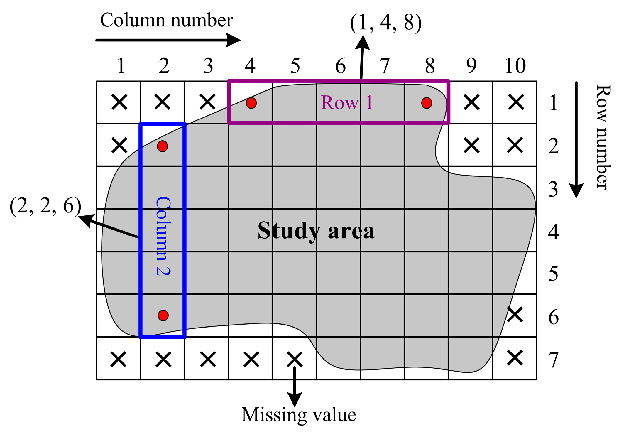
However, the original version of FullSWOF-2D was designed for rectangular areas [61]. We modified the code to make it available for irregular regions. Specifically, a data structure in C++ was set up, which recorded the row number or column number, as well as the serial numbers of the first and last valid cell of this row or column (Figure 2). This data structure marked the boundaries in four directions (i.e., left, right, top, and bottom) in the study area, aiding in the setting of boundary conditions.

2.2.2. 1D Subsurface Flow Module

One-dimensional vertical flow in Hydrus-1D is described by Richards’ equation [62]:
θ t = z K h h z + 1 S
where t is the time (min), θ is the volumetric water content (cm3/cm3), h is the soil water pressure head (cm), z is the spatial coordinate (cm) defined as positive upward, K ( h ) is the unsaturated hydraulic conductivity function (cm/min), and S is a source or sink term (cm/min).
Van Genuchten’s θ h and K h relationships are used to determine soil hydraulic properties in this model [63]:
θ h = θ r + θ s θ r 1 + α h n m          h 0
K h = K s S e 1 / 2 1 1 S e 1 / m m 2
where m = 1 1 / n , S e = θ θ r / θ s θ r , and θ r and θ s denote the residual and saturated volumetric water content (cm3/cm3), respectively; S e (-) is the relative saturation; α (cm−1), n (-), and m (-) are fitting parameters of the soil water characteristic curve.

2.2.3. Integrated Method

The integrated method used between surface water and subsurface water flow is the key part of an intergrated surface–subsurface flow model [64]. To coupld the 2D surface flow interactively with the 1D surbsurface flow, we apply the sequential head method proposed by Morita et al. [26,27,65]. The infiltration between two phases is used as the common internal boundary condition to be solved interactively, in which the potential infiltration capacity I p is calculated firstly. However, this variable, calculated using the original formula, shows a remarkable fluctuation during the receding process because of wet–dry transitions. In order to improve the continuity of the potential infiltration capacity, the infiltration is set as the Darcy flow between two vertically adjacent grids on the surface when there is surface ponding water, while the original formula is used when there is no ponding water. Therefore, the Darcy’s formulas for calculating potential infiltration capacity can be represented as follows:
I p = 0.5 K s + K 0 Y H 0 / Δ z          D = 0 0.5 K 0 + K 1 H 0 H 1 / Δ z       D > 0
where K s is the saturated hydraulic conductivity; K 0 and H 0 are the hydraulic conductivity and hydraulic head of the top node, respectively; K 1 and H 1 are the hydraulic conductivity and hydraulic head of the node below the top one, respectively; Δ z is the thickness of each discrete cell; D is the ponding water depth at a previous time step; and Y is the available water depth from rainfall and depth of flow at the surface, calculated as:
Y = r Δ t + D
where r is rainfall intensity and Δ t is the time increment. The water supply rate R s is calculated as:
R s = Y / Δ t = r + D / Δ t
At each time step, we compare R s with I p to determine the actual infiltration rate i and then set the corresponding boundary condition for the subsurface flow module. Further details can be found in the original work. Moreover, the surface flow module is not updated until the maximum surface ponding water depth on the field is larger than 0.1 mm [66], which can improve computional efficiency.

2.3. Modeling Cases

We first validated the surface flow module. Kirstetter’s artificial rainfall runoff experiment [67] and a classical V-sloping slope overland flow case [41] were selected as one-dimensional and two-dimensional cases, respectively. Secondly, the one-dimensional subsurface flow module was validated with a classical infiltration case in an unsaturated zone, as well as a typical rainfall event without surface runoff at the experimental field. Finally, a rainstorm event at the experimental field was simulated using the FullSWOF-Plain model. We evaluated the model performance using the Nash–Sutcliffe efficiency (NSE) [68] and root mean squared error (RMSE).

3. Results

3.1. Validation of the Surface Flow Module

3.1.1. One-Dimensional Outflow Case

Kirstetter’s artificial rainfall–runoff experiment [67] was selected as a one-dimensional outflow case. The test flume had a length of 4.04 m and width of 11.5 cm. The slope of the flume (So), as well as the artificial rainfall intensity (Irain), could be adjusted manually. The parameters of the three experimental cases are shown in Table 2.
The cell size was set as 0.05 m. The initial surface water depths and velocities were zero. The HLL2 flux and Manning’s formula were applied in this case. The CFL (Courant–Friedrichs–Lewy) factor was 0.4, and the Manning’s coefficient n was 0.025 s/m1/3. The minimum water depth hmin was set as 1 × 10⁻¹² m. A fictive cell was added adjacent to the outflow cell to improve computational stability [69,70]. The whole simulation duration was 1000 s, while the artificial rainfall lasted for the first 600 s. The results of this proposed model were consistent with those in Kirstetter’s work [67] (Figure 3).

3.1.2. Two-Dimensional Outflow Case

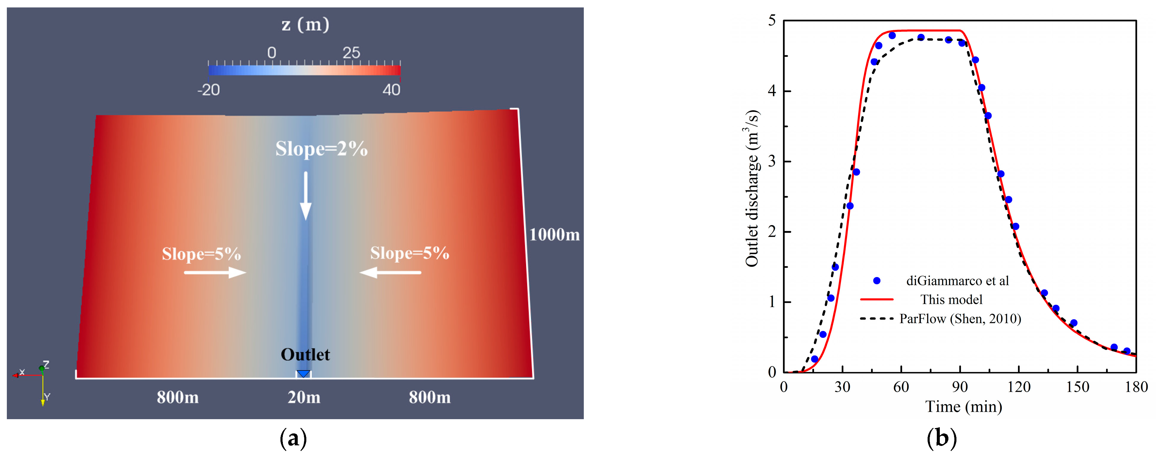
A classical tilted V-catchment overland flow case was chosen as the two-dimensional outflow case that was first proposed by Giammarco et al. [41] and then widely used in many articles [25,31,33,71,72,73]. A 20 m-wide low-lying channel was sandwiched between two symmetrical 1000 m × 800 m slopes. The slopes of two symmetrical slopes and the channel were 5% and 2%, respectively. We set the elevation of the top grid of the channel as 0 m, and the elevation of the whole area is shown in Figure 4a. The Manning’s coefficient n was 0.015 s/m1/3 for the valley side and 0.15 s/m1/3 for the channel. A constant spatial discretization of 20 m (Δx = Δy) was used. The critical depth condition was applied at the outlet. The rainfall intensity above the whole area was 10.8 mm/h, lasting for 90 min, with a total simulation time of 180 min. The CFL factor was 0.4. The simulated two-dimensional variables were output in the VTK (Visualization Tool Kit) data file format and then imported into ParaView software-4.3 (a visualization program for large 3-dimensional data sets) to export graphs.
We took Giammarco’s work [41] as a reference solution and compared the simulated hydrographs in the V-catchment of the three models (Figure 4b). The discharge predicted by our proposed model agreed well generally with those of Giammarco et al. [41] and ParFlow [37], especially during the receding limb. The outlet flux of our model was underestimated during the first 30 min, while the peak flow fitted better than that of ParFlow.

3.2. Validation of the Subsurface Flow Module

3.2.1. A Classical One-Dimensional Infiltration Case

A classical one-dimensional infiltration case was selected [74], which concerned vertical flow in the unsaturated zone. The length and width of the experimental soil column were both 50 cm, and the height was 200 cm. The bottom and top faces corresponded to the groundwater table and the soil surface, respectively (Figure 5a). The soil in this column was homogeneous, the saturated hydraulic conductivity K s was 10 cm/day, and the porosity n was 0.45. The constitutive relations of the soil were:
h h a 100 h a = 1 S w 1 S w r k r w = S w S w r 1 S w r
where k r w is relative hydraulic conductivity coefficient, S w r is residual water saturation, and h a is air entry value. As S w r was 0.333 and h a was 0, S w = 1 + 0.667 h / 100 and k r w = S w 0.333 / 0.667 .
The soil column was discretized into 40 cells, and the vertical cell size Δ z was 5 cm. The initial pressure head was 0 cm at the bottom, −90 cm at the soil surface, and −97 cm elsewhere. The rainfall intensity at the soil surface was 50 mm/day, lasting for 10 days. The time step was set as 0.1 day. The simulated profiles of pressure heads at different moments during infiltration were plotted in Figure 5b. Infiltration caused a gradual increase in pressure head values, starting from the top of the soil column. Generally, the numerical results obtained from this proposed model fitted reasonably well with UNSAT2 and Huyakorn’s model [74].

3.2.2. One-Dimensional Infiltration Case at the Experimental Field

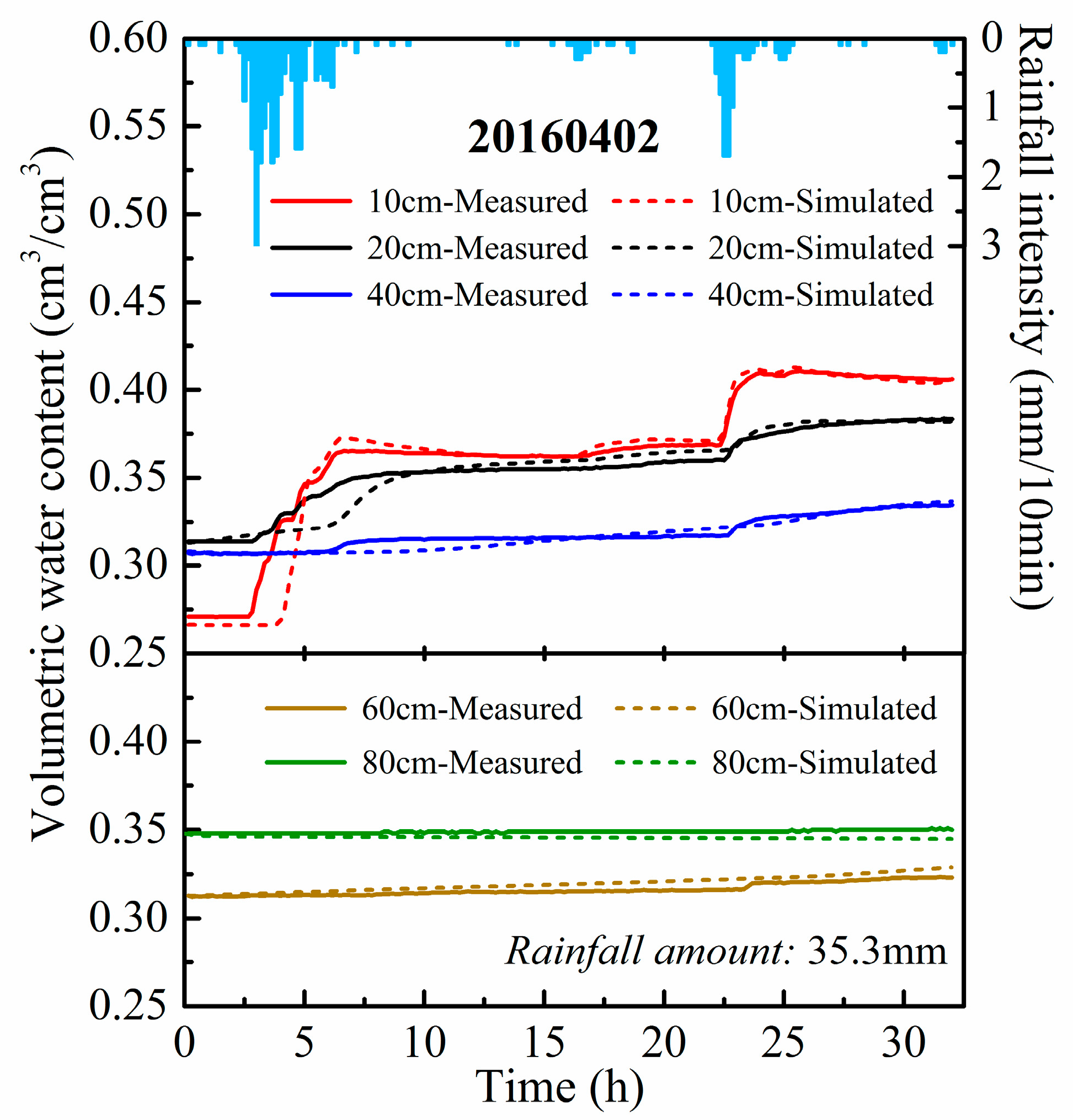
The soil moisture observation profile (10 cm, 20 cm, 40 cm, 60 cm, and 80 cm) in the experimental field could be conceptualized as a vertical soil column. We selected a typical light rainfall event (20160402) without surface runoff as the one-dimensional infiltration case. The total rainfall was 35.3 mm, and the initial groundwater depth was 1.13 m. The height of this soil column was set as 150 cm in the model, according to the initial groundwater depth. The vertical grid resolution was 1 cm. According to the characteristics of the genetic horizon and the buried depths of the five soil moisture probes, we divided the generalized soil profile into five layers, i.e., 0–13 cm, 13–22 cm, 22–47 cm, 47–75 cm, and 75–150 cm. Based on the measured parameters of the five layers (Table 1) and the hydraulic parameters in the van Genuchten model of a similar soil type [75,76], the calibrated parameters of the five layers are shown as Table 3. We ignored evaporation during the rainfall period.
The simulated soil moisture content at depths of 10 cm, 20 cm, 40 cm, 60 cm, and 80 cm were output (Figure 6). The simulated results fitted very well with the measured values. The RMSE values of soil moisture at all five depths were less than 0.03 cm3/cm3. However, the simulated response time of soil moisture above 40 cm depth lagged behind, which might be caused by abundant macropore pathways in the topsoil. During rainfall, a portion of the rainfall infiltrated rapidly into the subsoil through macropore-type preferential pathways. However, such a process was not considered in this subsurface module. We calculated the increment of soil moisture in each layer. Interestingly, more than 80 percents of the infiltration water was stored in the upper 40 cm soil layer, and almost one half was stored in the upper 10 cm soil layer. It was reasonable to only consider vertical infiltration in the unsaturated zone at the experimental field.

3.3. Validation of FullSWOF-Plain Model at Experimental Field

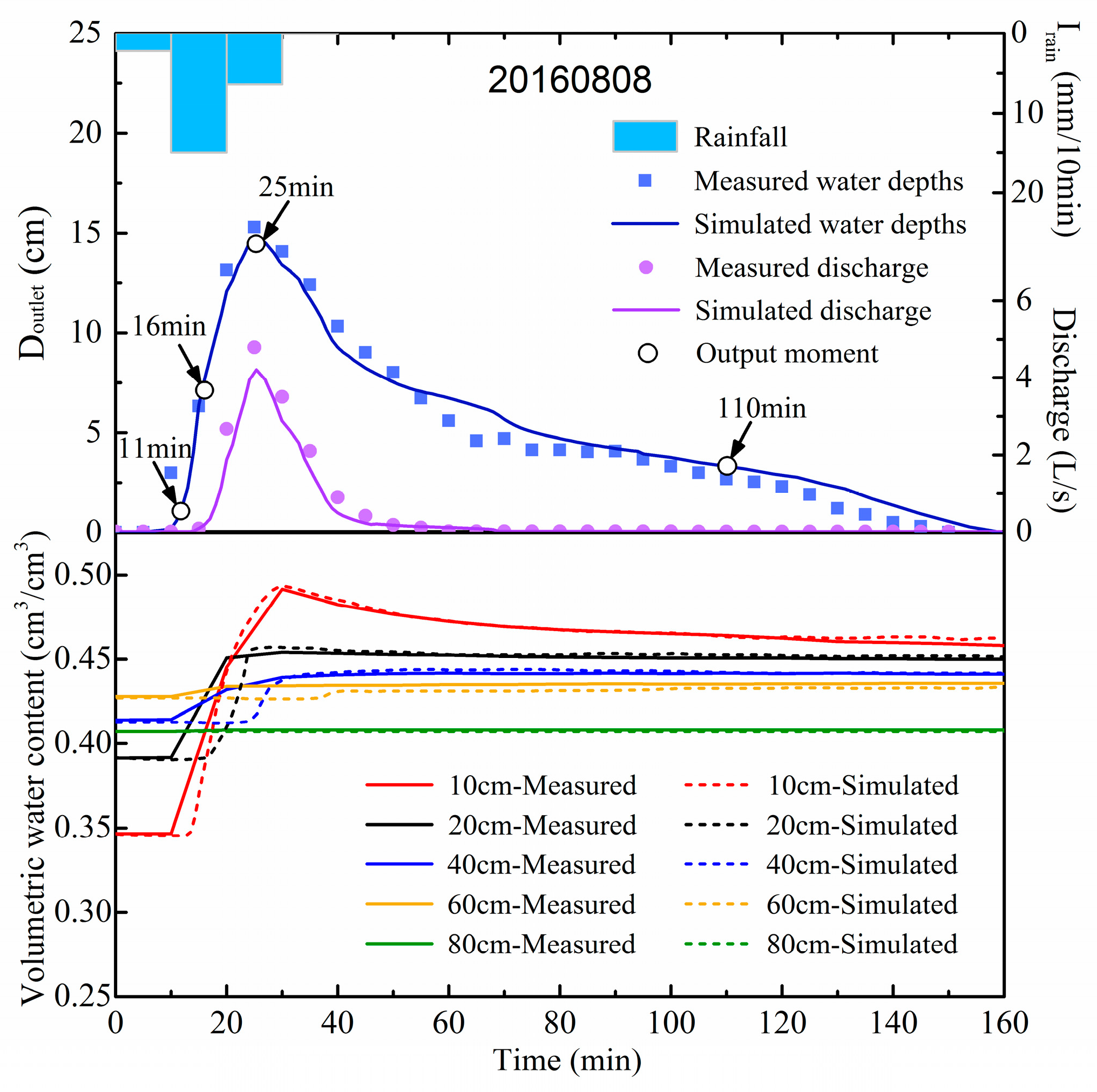
We simulated the rainfall runoff processes of the 20160808 rainfall event, which was known as a typical short-duration rainstorm. The rainfall was 23.7 mm, while the duration of the rainfall was around 30 min. The observed surface runoff was about 4.77 mm. Although fine-resolution DEMs can capture small-scale terrain structural features, they also cause an excessive computational burden. To balance simulation accuracy and efficiency, we chose a 0.3 m-resolution DEM, in which the number of effective discrete surface cells was 10,159 and the elevations varied from 2.73 m to 3.49 m. Hofer et al. [77] selected a similar spatial resolution (0.25 m) in the Chicken Creek basin (440 × 130 m). The elevation of the bottom boundary in the subsurface module was set as 2.29 m. The vertical grid resolution was 1 cm, with 889,052 effective discrete subsurface cells. The surface roughness coefficient was set as 0.02 s/m1/3 according to the range of bare land (0.018–0.06 s/m1/3) [78]. The time step of the subsurface flow module was 0.1 min, and a variable time step was applied in the surface flow module. The CFL factor was set as 0.8. The soil hydraulic parameters of the five layers in Table 3 were also applied in this case. Variables of h, u, v, and q were output every minute. The discharge was calculated from the water depth, using a water depth–discharge relation.
The simulated hydrograph and the soil moisture content at the five depths are shown in Figure 7. As the simulation period was too short to make the groundwater respond, we did not output the simulated groundwater depth. The discharge at the outlet reached a peak value at the 25th minute and then receded gradually. The simulated hydrograph agreed reasonably well with the measured hydrograph, while the simulated peak value was slightly lower than the measured one. The NSE and RMSE of the simulated water depth were 0.958 and 0.876 cm, respectively. The NSE and RMSE of the simulated discharge were 0.953 and 0.211 L/s, respectively. The simulated soil moisture content at the five depths fitted very well with the measured values. However, the simulated response time of soil moisture above an 80 cm depth clearly lagged, as expected. The deeper the soil depth was, the smaller the increment in soil moisture was. FullSWOF-Plain model was proven to be accurate and effective for simulating rainfall –runoff processes in the experimental field.
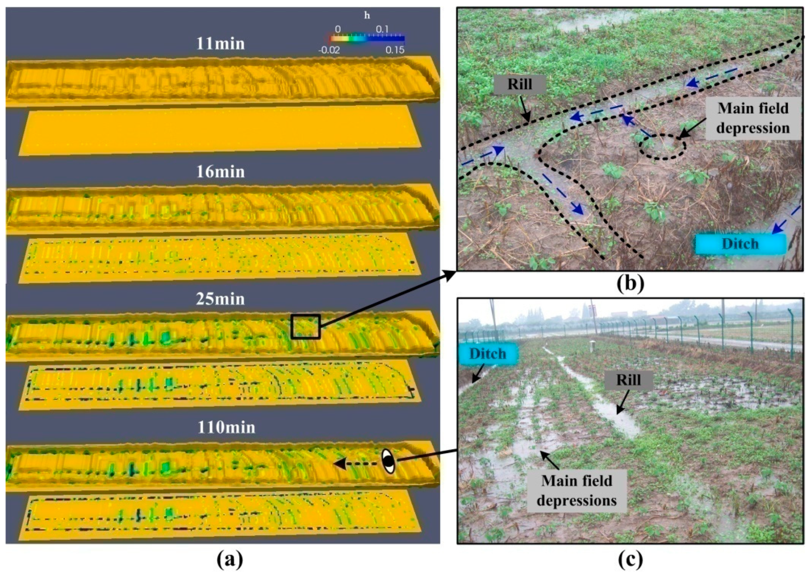
Furthermore, simulated ponding water depths at four typical moments, i.e., the 11th, 16th, 25th and 110th minutes, were output to figure out the characteristics of the runoff generation processes (Figure 8a). At the 11th minute, surface ponding water could only be seen in some scattered depressions in the ditch, with a tiny discharge at the outlet. Five minutes later (i.e., the 16th minute), the ponding water in the ditch increased rapidly. Meanwhile, ponding water could also clearly be found in many depressions in the main field. Subsequently, the discharge reached a peak value at the 25th minute. The surface ponding water depths at this moment were much deeper than those of the 16th minute. Remarkably, some adjacent scattered depressions in the main field connected, forming patches of puddles. These puddles also connected with the rills nearby, which connected with the surrounding ditch. Therefore, the excess surface water in the puddles drained into the ditch through the rills (Figure 8b). After the rainfall, the discharge receded gradually. At the 110th minute, the ponding water close to the outlet receded fastest, due to drainage. The ponding water of the puddles in the main field receded gradually due to infiltration, which made the connections of some puddles break (Figure 8c).

4. Discussion

This proposed model can accurately simulate rainfall runoff processes at a typical plot-scale plain farmland area with significant micro-topographic features. The visualization of temporal surface water distribution is crucial for understanding the mechanism of runoff generation. It can be seen from the whole rainfall runoff processes in rainfall event 20160808 that the micro-topography at multiple scales affected the ponding time and ponding areas greatly. Specifically, scattered surface ponding water first occurred in the ditch, which was the lowest part in the field, corresponding to the smallest soil water deficit. Then, surface ponding water could be seen in relatively low areas in the main field, which was higher than the ditch. Generally, lower local terrain experienced earlier surface ponding.
The concentration process of surface runoff presented hierarchical characteristics [10,79]. Obviously, the drainage ditch outflowed first, contributing the majority of the discharge during the early stage, which could be called the partial outflow period. As some adjacent scattered puddles in the main field connected, the excess surface water in the puddles drained into the ditch through some rills. Therefore, the initial partial outflow period turned into a whole-area outflow period. The main field contributed a large part of the outflow in the whole-area outflow period [80]. Overall, the micro-topography indeed affected the early outflow stage, while it impacted very little on surface runoff once the whole region outflowed [81].
Nevertheless, this proposed model could only be applied for rainfall event simulation recently, ignoring lateral subsurface flow and evaporation. We expect to introduce water balance theory to obtain a stable regional groundwater table after a single rainfall event, to make up for the role of lateral subsurface flow. Moreover, the evaporation condition will also be added into the model, so that this proposed model can be suitable for long-term simulation. Although Hydrus-1D proved reasonable for simulating the infiltration process in the experimental field, the response time of the simulated soil moisture clearly lagged because of the model neglecting the role of preferential flow. Therefore, it is necessary to incorporate the preferential flow process into the subsurface module in the future [36].
Even though our proposed model has been compared with ParFLOW in a two-dimensional outflow case and with UNSAT2 in a one-dimensional infiltration case, some more validation work needs to be conducted in the future, such as comparing its performance with well-known integrated surface–subsurface flow models (e.g., PIHM [32] and WASH123 [29]) in the experimental field. Furthermore, this model needs fine-resolution meshes even when it is applied in plot-scale areas, which definitely constrains the computational efficiency. It is necessary to introduce a GPUs (graphics processing units)-accelerated modeling framework into the model [82] in future studies, which will make it possible to achieve long-term simulation under fine-resolution meshes.

5. Conclusions

A new open-source integrated surface–subsurface flow model, FullSWOF-Plain model, was proposed, in which the one-dimensional subsurface module Hydrus-1D was integrated with a modified two-dimensional surface water flow module FullSWOF-2D via the sequential head method. Various experimental scenarios were simulated to validate the performance of this model, including two outflow cases (i.e., 1D and 2D) without infilration, a classical one-dimensional infiltration case, and two typical rainfall events in the experimental field. This proposed model could acquire high-accuracy simulated surface water depths, as well as layered soil moisture content, via applying 2D SWEs and the 1D Richards’ equation in the surface and subsurface flow modules, respectively. The key points are as follows:
(1)
The simulated results of this proposed model were accurate. The NSE of the simulated discharge exceeded 0.90 in the experimental field case, and the RMSE values for soil moisture at the five depths were consistently below 0.03 cm3/cm3. However, the simulated response time of soil moisture lagged due to the neglect of preferential flow.
(2)
Micro-topography at multiple scales greatly affected the ponding time and ponding areas. Lower local terrain normally experienced earlier surface ponding. Scattered surface ponding water initially occurred in the ditch and subsequently in the relatively low areas in the main field.
(3)
The concentration process of surface runoff exhibited hierarchical characteristics. The drainage ditch outflowed first, contributing the majority of the discharge during the early stage. As some adjacent scattered puddles in the main field connected, the excess surface water in these puddles drained into the ditch through rills.

Author Contributions

Data curation, H.Y. (Hai Yang); Methodology, H.Y. (Hai Yang); Project administration, Q.Z. and Y.J.; Supervision, Q.Z. and Y.J.; Validation, H.Y. (Hai Yang); Writing—original draft, H.Y. (Hai Yang) and L.H.; Writing—review and editing, Q.Z., L.H., H.Y. (Hui Yang) and Q.Q. All authors have read and agreed to the published version of the manuscript.

Funding

This research was funded by the China Geological Survey Program (DD20221728) and the National Key Research and Development Program of China (No. 2022YFC3705001).

Data Availability Statement

Data are available on request from the authors.

Acknowledgments

We thank Congcong Jiao and Chengcheng Zhang for assistance in optimizing the model structure.

Conflicts of Interest

Author Hui Yang was employed by the company Guangdong Bangpu Recycling Technology Company Limited. The remaining authors declare that the research was conducted in the absence of any commercial or financial relationships that could be construed as a potential conflict of interest.

References

  1. Yan, R.; Li, L.; Gao, J. Framework for quantifying rural NPS pollution of a humid lowland catchment in Taihu Basin, Eastern China. Sci. Total Environ. 2019, 688, 983–993. [Google Scholar] [CrossRef] [PubMed]
  2. Appels, W.M.; Bogaart, P.W.; van der Zee, S.E.A.T.M. Feedbacks Between Shallow Groundwater Dynamics and Surface Topography on Runoff Generation in Flat Fields. Water Resour. Res. 2017, 53, 10336–10353. [Google Scholar] [CrossRef]
  3. Van der Ploeg, M.J.; Appels, W.M.; Cirkel, D.G.; Oosterwoud, M.R.; Witte, J.-P.M.; van der Zee, S.E.A.T.M. Microtopography as a Driving Mechanism for Ecohydrological Processes in Shallow Groundwater Systems. Vadose Zone J. 2012, 11, 811–822. [Google Scholar] [CrossRef]
  4. Planchon, O.; Esteves, M.; Silvera, N.; Lapetite, J.-M. Microrelief induced by tillage: Measurement and modelling of Surface Storage Capacity. Catena 2001, 46, 141–157. [Google Scholar] [CrossRef]
  5. Frei, S.; Fleckenstein, J.H. Representing effects of micro-topography on runoff generation and sub-surface flow patterns by using superficial rill/depression storage height variations. Environ. Model. Softw. 2014, 52, 5–18. [Google Scholar] [CrossRef]
  6. Habtezion, N.; Nasab, M.T.; Chu, X. How Does DEM Resolution Affect Microtopographic Characteristics, Hydrologic Connectivity, and Modeling of Hydrologic Processes? Hydrol. Process. 2016, 30, 4870–4892. [Google Scholar] [CrossRef]
  7. Appels, W.M.; Bogaart, P.W.; van der Zee, S.E.A.T.M. Influence of spatial variations of microtopography and infiltration on surface runoff and field scale hydrological connectivity. Adv. Water Resour. 2011, 34, 303–313. [Google Scholar] [CrossRef]
  8. Carvajal, F.; Aguilar, M.A.; Agüera, F.; Aguilar, F.J.; Giráldez, J.V. Maximum Depression Storage and Surface Drainage Network in Uneven Agricultural Landforms. Biosyst. Eng. 2006, 95, 281–293. [Google Scholar] [CrossRef]
  9. Hansen, B. Estimation of surface runoff and water-covered area during filling of surface microrelief depressions. Hydrol. Process. 2000, 14, 1235–1243. [Google Scholar] [CrossRef]
  10. Chu, X.; Yang, J.; Chi, Y.; Zhang, J. Dynamic puddle delineation and modeling of puddle-to-puddle filling-spilling-merging-splitting overland flow processes. Water Resour. Res. 2013, 49, 3825–3829. [Google Scholar] [CrossRef]
  11. Appels, W.M.; Bogaart, P.W.; van der Zee, S.E.A.T.M. Surface runoff in flat terrain: How field topography and runoff generating processes control hydrological connectivity. J. Hydrol. 2016, 534, 493–504. [Google Scholar] [CrossRef]
  12. Frei, S.; Lischeid, G.; Fleckenstein, J.H. Effects of micro-topography on surface–subsurface exchange and runoff generation in a virtual riparian wetland—A modeling study. Adv. Water Resour. 2010, 33, 1388–1401. [Google Scholar] [CrossRef]
  13. Freeze, R.A.; Harlan, R.L. Blueprint for a physically-based, digitally-simulated hydrologic response model. J. Hydrol. 1969, 9, 237–258. [Google Scholar] [CrossRef]
  14. Ebel, B.A.; Loague, K. Physics-based hydrologic-response simulation: Seeing through the fog of equifinality. Hydrol. Process. 2006, 20, 2887–2900. [Google Scholar] [CrossRef]
  15. Paniconi, C.; Putti, M. Physically based modeling in catchment hydrology at 50: Survey and outlook. Water Resour. Res. 2015, 51, 7090–7129. [Google Scholar] [CrossRef]
  16. Loague, K.; VanderKwaak, J.E. Physics-based hydrologic response simulation: Platinum bridge, 1958 Edsel, or useful tool. Hydrol. Process. 2004, 18, 2949–2956. [Google Scholar] [CrossRef]
  17. Kampf, S.K.; Burges, S.J. A framework for classifying and comparing distributed hillslope and catchment hydrologic models. Water Resour. Res. 2007, 43, W05423. [Google Scholar] [CrossRef]
  18. Furman, A. Modeling coupled surface-subsurface flow processes: A review. Vadose Zone J. 2008, 7, 741–756. [Google Scholar] [CrossRef]
  19. Sebben, M.L.; Werner, A.D.; Liggett, J.E.; Partington, D.; Simmons, C.T. On the testing of fully integrated surface–subsurface hydrological models. Hydrol. Process. 2013, 27, 1276–1285. [Google Scholar] [CrossRef]
  20. Refsgaard, J.C.; Stisen, S.; Koch, J. Hydrological process knowledge in catchment modelling—Lessons and perspectives from 60 years development. Hydrol. Process. 2022, 36, e14463. [Google Scholar] [CrossRef]
  21. Ebel, B.A.; Loague, K.; Vanderkwaak, J.E.; Dietrich, W.E.; Montgomery, D.R.; Torres, R.; Anderson, S.P. Near-surface hydrologic response for a steep, unchanneled catchment near Coos Bay, Oregon: 2. Physics-based simulations. Am. J. Sci. 2007, 307, 709–748. [Google Scholar] [CrossRef]
  22. Mirus, B.B.; Loague, K.; VanderKwaak, J.E.; Kampf, S.K.; Burges, S.J. A hypothetical reality of Tarrawarra-like hydrologic response. Hydrol. Process. 2009, 23, 1093–1103. [Google Scholar] [CrossRef]
  23. Abbott, M.B.; Bathurst, J.C.; Cunge, J.A.; O’Connell, P.E.; Rasmussen, J. An introduction to the European Hydrological System—Systeme Hydrologique Europeen, “SHE”, 1: History and philosophy of a physically-based, distributed modelling system. J. Hydrol. 1986, 87, 45–59. [Google Scholar] [CrossRef]
  24. Abbott, M.B.; Bathurst, J.C.; Cunge, J.A.; O’Connell, P.E.; Rasmussen, J. An introduction to the European Hydrological System—Systeme Hydrologique Europeen, “SHE”, 2: Structure of a physically-based, distributed modelling system. J. Hydrol. 1986, 87, 61–77. [Google Scholar] [CrossRef]
  25. VanderKwaak, J.E. Numerical Simulation of Flow and Chemical Transport in Integrated Surface-Subsurface Hydrologic Systems; University of Waterloo: Waterloo, ON, Canada, 1999. [Google Scholar]
  26. Morita, M.; Chie Yen, B. Numerical methods for conjunctive two-dimensional surface and three-dimensional sub-surface flows. Int. J. Numer. Methods Fluids 2000, 32, 921–957. [Google Scholar] [CrossRef]
  27. Morita, M.; Yen, B.C. Modeling of conjunctive two-dimensional surface-three-dimensional subsurface flows. J. Hydraul. Eng. 2002, 128, 184–200. [Google Scholar] [CrossRef]
  28. Panday, S.; Huyakorn, P.S. A fully coupled physically-based spatially-distributed model for evaluating surface/subsurface flow. Adv. Water Resour. 2004, 27, 361–382. [Google Scholar] [CrossRef]
  29. Yeh, G.T.; Huang, G.B.; Zhang, F.; Lin, H.C.; Edris, E.; Richards, D. A Numerical Model of Flow, Heat transfer, and Salinity, Sediment, and Water Quality Transport in Watershed Systems of 1-D Stream-River Network, 2-D Overland Regime, and 3D Subsurface Media (WASH123D: Version 2.0); U.S. Army Corps of Eng: Vicksburg, MI, USA, 2004. [Google Scholar]
  30. Therrien, R.; McLaren, R.G.; Sudicky, E.A.; Panday, S.M. HydroGeoSphere-A Three-Dimensional Numerical Model Describing Fully-Integrated Subsurface and Surface Flow and Solute Transport; Groundwater Simulations Group: Waterloo, ON, Canada, 2010. [Google Scholar]
  31. Kollet, S.J.; Maxwell, R.M. Integrated surface–groundwater flow modeling: A free-surface overland flow boundary condition in a parallel groundwater flow model. Adv. Water Resour. 2006, 29, 945–958. [Google Scholar] [CrossRef]
  32. Qu, Y.; Duffy, C.J. A semidiscrete finite volume formulation for multiprocess watershed simulation. Water Resour. Res. 2007, 43, W08419. [Google Scholar] [CrossRef]
  33. He, Z.; Wu, W.; Wang, S.S. Coupled Finite-Volume Model for 2D Surface and 3D Subsurface Flows. J. Hydrol. Eng. 2008, 13, 835–845. [Google Scholar] [CrossRef]
  34. Kumar, M.; Duffy, C.J.; Salvage, K.M. A Second-Order Accurate, Finite Volume–Based, Integrated Hydrologic Modeling (FIHM) Framework for Simulation of Surface and Subsurface Flow. Vadose Zone J. 2009, 8, 873–890. [Google Scholar] [CrossRef]
  35. Kolditz, O.; Bauer, S.; Bilke, L.; Böttcher, N.; Delfs, J.O.; Fischer, T.; Görke, U.J.; Kalbacher, T.; Kosakowski, G.; McDermott, C.I.; et al. OpenGeoSys: An open-source initiative for numerical simulation of thermo-hydro-mechanical/chemical (THM/C) processes in porous media. Environ. Earth Sci. 2012, 67, 589–599. [Google Scholar] [CrossRef]
  36. Warsta, L.; Taskinen, A.; Koivusalo, H.; Paasonen-Kivekäs, M.; Karvonen, T. Modelling soil erosion in a clayey, subsurface-drained agricultural field with a three-dimensional FLUSH model. J. Hydrol. 2013, 498, 132–143. [Google Scholar] [CrossRef]
  37. Shen, C.; Phanikumar, M.S. A process-based, distributed hydrologic model based on a large-scale method for surface–subsurface coupling. Adv. Water Resour. 2010, 33, 1524–1541. [Google Scholar] [CrossRef]
  38. Shokri, A.; Bardsley, W.E. Development, testing and application of DrainFlow: A fully distributed integrated surface-subsurface flow model for drainage study. Adv. Water Resour. 2016, 92, 299–315. [Google Scholar] [CrossRef]
  39. De Maet, T.; Cornaton, F.; Hanert, E. A scalable coupled surface–subsurface flow model. Comput. Fluids 2015, 116, 74–87. [Google Scholar] [CrossRef]
  40. Tian, D.f.; Zheng, H.; Liu, D.f. A 2D integrated FEM model for surface water–groundwater flow of slopes under rainfall condition. Landslides 2017, 14, 577–593. [Google Scholar] [CrossRef]
  41. Giammarco, P.D.; Todini, E.; Lamberti, P. A conservative finite elements approach to overland flow: The control volume finite element formulation. J. Hydrol. 1996, 175, 267–291. [Google Scholar] [CrossRef]
  42. Lighthill, M.J.; Whitham, G.B. On Kinematic Waves. I. Flood Movement in Long Rivers. Proc. R. Soc. Lond. A Math. Phys. Eng. Sci. 1955, 229, 281–316. [Google Scholar]
  43. Costabile, P.; Costanzo, C.; Macchione, F. Comparative analysis of overland flow models using finite volume schemes. J. Hydroinformatics 2012, 14, 122–135. [Google Scholar] [CrossRef]
  44. Yeh, G.-T.; Shih, D.-S.; Cheng, J.-R.C. An integrated media, integrated processes watershed model. Comput. Fluids 2011, 45, 2–13. [Google Scholar] [CrossRef]
  45. Zhou, Q.Y.; Shimada, J.; Sato, A. Temporal variations of the three-dimensional rainfall infiltration process in heterogeneous soil. Water Resour. Res. 2002, 38, 1-1–1-15. [Google Scholar] [CrossRef]
  46. Singh, J.; Altinakar, M.S.; Ding, Y. Numerical Modeling of Rainfall-Generated Overland Flow Using Nonlinear Shallow-Water Equations. J. Hydrol. Eng. 2015, 20, 04014089. [Google Scholar] [CrossRef]
  47. Simons, F.; Busse, T.; Hou, J.; Özgen, I.; Hinkelmann, R. A model for overland flow and associated processes within the Hydroinformatics Modelling System. J. Hydroinformatics 2014, 16, 375–391. [Google Scholar] [CrossRef]
  48. Fiedler, F.R.; Ramirez, J.A. A numerical method for simulating discontinuous shallow flow over an infiltrating surface. Int. J. Numer. Methods Fluids 2000, 32, 219–239. [Google Scholar] [CrossRef]
  49. Esteves, M.; Faucher, X.; Galle, S.; Vauclin, M. Overland flow and infiltration modelling for small plots during unsteady rain: Numerical results versus observed values. J. Hydrol. 2000, 228, 265–282. [Google Scholar] [CrossRef]
  50. Delestre, O.; Darboux, F.; James, F.; Lucas, C.; Laguerre, C.; Cordier, S. FullSWOF: A free software package for the simulation of shallow water flows. arXiv 2014, arXiv:1401.4125. [Google Scholar]
  51. Fernández-Pato, J.; Caviedes-Voullième, D.; García-Navarro, P. Rainfall/runoff simulation with 2D full shallow water equations: Sensitivity analysis and calibration of infiltration parameters. J. Hydrol. 2016, 536, 496–513. [Google Scholar] [CrossRef]
  52. Caviedes-Voullième, D.; García-Navarro, P.; Murillo, J. Influence of mesh structure on 2D full shallow water equations and SCS Curve Number simulation of rainfall/runoff events. J. Hydrol. 2012, 448-449, 39–59. [Google Scholar] [CrossRef]
  53. Delestre, O. Rain Water Overland Flow on Agricultural Fields Simulation; Université d’Orléans: Orléans, France, 2010. [Google Scholar]
  54. Unterweger, K.; Wittmann, R.; Neumann, P.; Weinzierl, T.; Bungartz, H.-J. Integration of FULLSWOF2D and PeanoClaw: Adaptivity and Local Time-Stepping for Complex Overland Flows. In Recent Trends in Computational Engineering—CE2014: Optimization, Uncertainty, Parallel Algorithms, Coupled and Complex Problems; Mehl, M., Bischoff, M., Schäfer, M., Eds.; Springer International Publishing: Cham, Switzerland, 2015; pp. 181–195. [Google Scholar]
  55. Nurritasari, F.A.; Sudibyakto, S.; Jetten, V.G. OpenLISEM Flash Flood Modelling Application in Logung Sub-Catchment, Central Java. Indones. J. Geogr. 2015, 47, 132–141. [Google Scholar] [CrossRef]
  56. Li, X.; Wang, C.; Chen, G.; Wang, Q.; Hu, Z.; Wu, J.; Wang, S.; Fang, X. Evaluating Efficiency Improvement of Deep-Cut Curb Inlets for Road-Bioretention Stripes. Water 2020, 12, 3368. [Google Scholar] [CrossRef]
  57. Hao, X.; Li, Y.; Liu, S. Comparison of dynamic flow interaction methods between pipe system and overland in urban flood analysis. Sci. Rep. 2021, 11, 12079. [Google Scholar] [CrossRef] [PubMed]
  58. Genuchten, B.V. HYDRUS-1D code for simulating the one-dimensional movement of water, heat, and multiple solutes in variably saturated media. In Proceedings of the International Ground Water Modeling Center, Colorado School of Mines, Golden, CO, USA, 4–8 October 1998. [Google Scholar]
  59. Simunek, J.; Van Genuchten, M.T.; Sejna, M. The HYDRUS-1D Software Package for Simulating the One-Dimensional Movement of Water, Heat, and Multiple Solutes in Variably-Saturated Media; U.S. Salinity Laboratory Agricultural Research Service, U.S. Department of Agriculture: Riverside, CA, USA, 2005; Volume 3, pp. 1–240. [Google Scholar]
  60. Šimůnek, J.; van Genuchten, M.T.; Šejna, M. Recent Developments and Applications of the HYDRUS Computer Software Packages. Vadose Zone J. 2016, 15, vzj2016.04.0033. [Google Scholar] [CrossRef]
  61. Tatard, L.; Planchon, O.; Wainwright, J.; Nord, G.; Favis-Mortlock, D.; Silvera, N.; Ribolzi, O.; Esteves, M.; Huang, C.H. Measurement and modelling of high-resolution flow-velocity data under simulated rainfall on a low-slope sandy soil. J. Hydrol. 2008, 348, 1–12. [Google Scholar] [CrossRef]
  62. Richards, L.A. Capillary conduction of liquids through porous mediums. J. Appl. Phys. 1931, 1, 318–333. [Google Scholar] [CrossRef]
  63. van Genuchten, M.T. A Closed-form Equation for Predicting the Hydraulic Conductivity of Unsaturated Soils. Soil Sci. Soc. Am. J. 1980, 44, 892–898. [Google Scholar] [CrossRef]
  64. Huang, G.; Yeh, G.-T. Comparative Study of Coupling Approaches for Surface Water and Subsurface Interactions. J. Hydrol. Eng. 2009, 14, 453–462. [Google Scholar] [CrossRef]
  65. Morita, M.; Yen, B.C. Study on interaction between surface and subsurface flows using conjunctive flow model. In Ground Water Updates; Sato, K., Iwasa, Y., Eds.; Springer: Berlin/Heidelberg, Germany, 2000; pp. 265–270. [Google Scholar]
  66. Brown, D.L. An Analysis of Transient Flow in Upland Watersheds: Interactions between Structure and Process; University of California: Berkeley, CA, USA, 1995. [Google Scholar]
  67. Kirstetter, G.; Hu, J.; Delestre, O.; Darboux, F.; Lagrée, P.Y.; Popinet, S.; Fullana, J.M.; Josserand, C. Modeling rain-driven overland flow: Empirical versus analytical friction terms in the shallow water approximation. J. Hydrol. 2016, 536, 1–9. [Google Scholar] [CrossRef]
  68. Nash, J.E.; Sutcliffe, J.V. RiverRiver flow forecasting through conceptual models part I—A discussion of principles. J. Hydrol. 1970, 10, 282–290. [Google Scholar] [CrossRef]
  69. Bradford, S.F.; Katopodes, N.D. Hydrodynamics of Turbid Underflows.I: Formulation and Numerical Analysis. J. Hydraul. Eng. 1999, 125, 1006–1015. [Google Scholar] [CrossRef]
  70. Sanders, B.F. High-resolution and non-oscillatory solution of the St. Venant equations in non-rectangular and non-prismatic channels. J. Hydraul. Res. 2001, 39, 321–330. [Google Scholar] [CrossRef]
  71. Shen, C. A Process-Based Distributed Hydrologic Model and Its Application to a Michigan Watershed; Michigan State University: East Lansing, MI, USA, 2009. [Google Scholar]
  72. Weill, S.; Mouche, E.; Patin, J. A generalized Richards equation for surface/subsurface flow modelling. J. Hydrol. 2009, 366, 9–20. [Google Scholar] [CrossRef]
  73. Tian, D.; Liu, D. A new integrated surface and subsurface flows model and its verification. Appl. Math. Model. 2011, 35, 3574–3586. [Google Scholar] [CrossRef]
  74. Huyakorn, P.S.; Springer, E.P.; Guvanasen, V.; Wadsworth, T.D. A three-dimensional finite-element model for simulating water flow in variably saturated porous media. Water Resour. Res. 1986, 22, 1790–1808. [Google Scholar] [CrossRef]
  75. Tan, X.; Shao, D.; Gu, W.; Liu, H. Field analysis of water and nitrogen fate in lowland paddy fields under different water managements using HYDRUS-1D. Agr. Water Manag. 2015, 150, 67–80. [Google Scholar] [CrossRef]
  76. Carsel, R.F.; Parrish, R.S. Developing joint probability distributions of soil water retention characteristics. Water Resour. Res. 1988, 24, 755–769. [Google Scholar] [CrossRef]
  77. Hofer, M.; Lehmann, P.; Biemelt, D.; Stähli, M.; Krafczyk, M. Modelling subsurface drainage pathways in an artificial catchment. Phys. Chem. Earth Parts A/B/C 2011, 36, 101–112. [Google Scholar] [CrossRef]
  78. Chow, V.T. Open-Channel Hydraulics; MaGraw-Hill: Tokyo, Japan, 1959; p. 680. [Google Scholar]
  79. Yang, J.; Chu, X. Quantification of the spatio-temporal variations in hydrologic connectivity of small-scale topographic surfaces under various rainfall conditions. J. Hydrol. 2013, 505, 65–77. [Google Scholar] [CrossRef]
  80. Yang, H.; Jiang, Y.; Zhou, Q.; Yang, H.; Ma, Q.; Zhang, C.; Wang, C. Effects of Microtopography on Runoff Generation in Plain Farmland: New Insights from an Event-Based Rainfall–Runoff Model. Water 2022, 14, 2686. [Google Scholar] [CrossRef]
  81. Chen, L.; Sela, S.; Svoray, T.; Assouline, S. The role of soil-surface sealing, microtopography, and vegetation patches in rainfall-runoff processes in semiarid areas. Water Resour. Res. 2013, 49, 5585–5599. [Google Scholar] [CrossRef]
  82. Buttinger-Kreuzhuber, A.; Konev, A.; Horváth, Z.; Cornel, D.; Schwerdorf, I.; Blöschl, G.; Waser, J. An integrated GPU-accelerated modeling framework for high-resolution simulations of rural and urban flash floods. Env. Model. Softw. 2022, 156, 105480. [Google Scholar] [CrossRef]
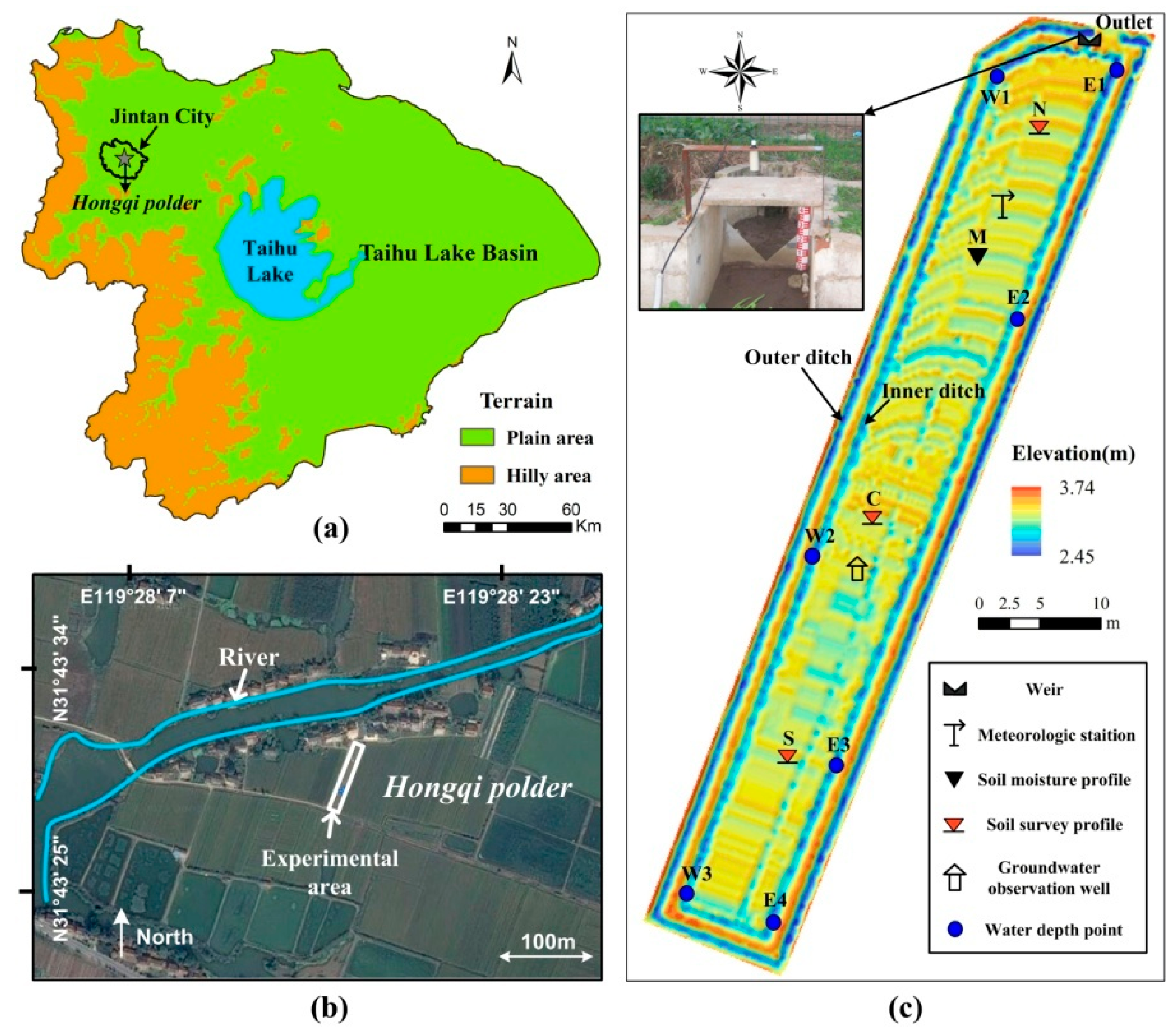
Figure 1. Overview of study area: (a) location of Hongqi polder; (b) location of study area; (c) topography and observation instrument of study area.
Water 16 01528 g001
Figure 2. A schematic of marking boundary information with a data structure in an irregular study area.
Water 16 01528 g002
Figure 3. (ac) Observed and simulated hydrographs of three experimental cases.
Water 16 01528 g003
Figure 4. Two–dimensional outflow case: (a) terrain of tilled V-catchment; (b) simulation results of three models, including Giammarco et al. [41], ParFlow [37] and this model.
Water 16 01528 g004
Figure 5. One–dimensional infiltration case: (a) initial and boundary conditions of soil column; (b) computed pressure head profiles during infiltration of Huyakorn’s model [74] (dotted lines), this proposed model (solid lines), and UNSAT2 (points).
Water 16 01528 g005
Figure 6. Simulated results of layered soil moisture content in rainfall event 20160402 at experimental field.
Water 16 01528 g006
Figure 7. Simulated results of experimental field in rainstorm event 20160808.
Water 16 01528 g007
Figure 8. Simulated results of rainstorm event 20160808: (a) simulated ponding water depths on field at four typical moments; (b) image of concentration process on field; (c) image of field at 110th minute.
Water 16 01528 g008
Table 1. The measured physical and hydraulic parameters of the five soil layers.
Depth (cm)Clay
(-)
Silt
(-)
ρ b
(g/cm3)
n
(-)
K s
(cm/min)
0–100.31 (0.27–0.34)0.57 (0.53–0.62)1.20 (1.10–1.28)0.55 (0.52–0.58)0.07 (0.02–0.25)
10–200.29 (0.26–0.34)0.61 (0.58–0.64)1.23 (1.05–1.50)0.50 (0.43–0.60)0.08 (0.01–0.22)
20–400.29 (0.26–0.32)0.63 (0.61–0.67)1.47 (1.41–1.50)0.45 (0.43–0.47)0.07 (0.02–0.13)
40–600.33 (0.30–0.35)0.61 (0.58–0.64)1.46 (1.35–1.53)0.45 (0.42–0.49)0.11 (0.04–0.18)
60–800.41 (0.38–0.43)0.54 (0.53–0.58)1.46 (1.41–1.50)0.45 (0.42–0.47)0.03 (0.01–0.05)
Table 2. Main parameters of three experimental cases.
Case NumberRainfall Intensity Irain (mm/h)Slope So (%)
1502
2252
3255
Table 3. Calibrated soil hydraulic parameters in van Genuchten model of five layers in subsurface module.
Depth (cm) θ s (cm3/cm3) θ r (cm3/cm3) α (cm−1) n (-) K s
0–13 0.4950.0900.0101.250.05
13–22 0.4550.1000.0081.150.03
22–47 0.4450.0900.0101.200.03
47–75 0.4350.0700.0111.200.03
75–150 0.4050.0700.0111.150.02
Disclaimer/Publisher’s Note: The statements, opinions and data contained in all publications are solely those of the individual author(s) and contributor(s) and not of MDPI and/or the editor(s). MDPI and/or the editor(s) disclaim responsibility for any injury to people or property resulting from any ideas, methods, instructions or products referred to in the content.