Article

Hydraulic Transient Impact on Surrounding Rock Mass of Unlined Pressure Tunnels

by
Sanyam Ghimire
1,*,
Krishna Kanta Panthi
1 and
Kaspar Vereide
2
1
Department of Geoscience and Petroleum, Norwegian University of Science and Technology (NTNU), Petroleumsteknisk Senter, F 410, Valgrinda, S.P. Andersens Vei 15a, 7031 Trondheim, Norway
2
Department of Civil and Environmental Engineering, Norwegian University of Science and Technology (NTNU), Vassbygget, 322, Valgrinda, S.P. Andersens Veg 5, 7031 Trondheim, Norway
*
Author to whom correspondence should be addressed.
Water 2023, 15(22), 3894; https://doi.org/10.3390/w15223894
Submission received: 7 October 2023 / Revised: 31 October 2023 / Accepted: 6 November 2023 / Published: 8 November 2023
(This article belongs to the Section Hydraulics and Hydrodynamics)

Abstract

:
The frequent pressure pulsations due to hydraulic transients in hydropower plants induce cyclic loading on the rock mass that may contribute to increased instances of block falls and increased risk of tunnel collapse over the power plant lifetime. This study focuses on understanding the effect of frequent start and stop sequences of hydropower in unlined pressure tunnels. For this purpose, data from a pore water pressure monitoring system is utilized, which was installed at the downstream end of the headrace tunnel at the 50 MW Roskrepp hydropower plant in southern Norway. The objective of this study is to analyze the recorded data and quantify the impact of the hydraulic transient on the surrounding rock mass in the unlined pressure tunnel. The monitoring of pressure data over several years clearly shows that frequent load changes could cause a considerable effect on the rock mass and constituent joint system. A delayed response of the pressure in boreholes in the rock mass compared with inside the tunnel is seen in all start and stop sequences and is considered to be the main reason for instability caused by transients. The response of pore pressure in boreholes is greatly influenced by the characteristics of joints. The results show that the start sequence and shorter shutdown duration exert a greater impact on rock mass as compared to the stop sequence and longer shutdown duration. Therefore, it is recommended to increase the shutdown duration so that the impact can be minimized to increase the tunnel lifetime. This study recommends implementing a more conservative design approach in tunnels with weak rock masses in projects that involve frequent load changes.

1. Introduction

Hydropower has been a source of electricity since the late 19th century. Over the years, hydropower projects have been developed in diverse geological and topographical settings with various layouts. In Norway, most of the hydropower projects utilize unlined pressure tunnels as the primary waterway system, spanning a total length of over 4300 km and operating at high heads, with the highest at 1047 m [1]. The growing need for electricity has driven the industry to start projects with unlined pressure tunnels in places with difficult geological conditions worldwide [2]. The tunnels are designed to withstand the pressure exerted by the water on the surrounding rock mass of the tunnel. Rock support is only provided where it is deemed necessary, i.e., in areas where the rock mass is too weak to withstand the internal water pressure. In addition, penstock lining is applied to a relatively short section of the pressure tunnel near the powerhouse area.
In the past, most of the hydropower plants in Norway operated primarily as base load energy supply systems where high-pressure unlined tunnels and shafts were designed primarily considering the maximum static water head as the main parameter. Deregulation of the energy market in 1991 [3] brought changes to their operational patterns, with hydropower plants adapting to market signals with the supply for the demand of electrical energy. This led to an increase in the start and stop sequences of regulated hydropower plants in Norway, known as “hydropeaking”, due to rapid adjustments to the discharge in turbines to meet varying market demands. With the growing penetration of renewable and unregulated energy sources, such as solar and wind, the operational regime of hydropower plants shifted from base load to peaking in the energy market. To maintain a balance between electricity production and consumption, flexibility in power production and storage systems became crucial. Regulated hydropower offers both short and long-term flexibility, where Norwegian hydropower reservoirs play a vital role [4,5,6] in providing reliable, flexible and balanced energy supply in the Nordic region. The pursuit of making hydropower more flexible has resulted in an increase in operational variability (start and stop) of the power plants. In recent years, there has been an increasing trend of start–stop sequences in the Norwegian hydropower plants. It is projected that the average number of start–stop sequences may increase by 30–45% between 2025 and 2040 in Norwegian hydropower plants [7]. Consequently, there will likely be a higher frequency and intensity of load changes, leading to more frequent and stronger transients in the future.
The inspections carried out in the pressure tunnels and shafts in recent years clearly indicate that the varying cyclic load has resulted in intensified block falls. In this context, unlined pressure tunnels and shafts will experience even more block falls resulting from cyclic load induced by increased dynamic operation of hydropower plants [8,9]. This is because new joints are formed or existing joints are extended due to exceeded fatigue strength of rock mass, which results in the creation of an intact rock bridge leading to a wedge failure in the periphery of the tunnel. Therefore, a better understanding of transients and their impact on surrounding rock mass is deemed necessary.
According to the state-of-the-art design criteria for unlined tunnels, minor rock falls are considered acceptable as long as they do not have a notable impact on frictional loss or result in tunnel blockage. The Norwegian pressure tunnel and shaft design methods have undergone various upgrades such as criteria for overburden and length along with topography correction and more than one valley consideration [1,10]. Design of unlined pressure tunnels and shafts also includes confinement criteria assisted by in situ rock stress measurement with validation using 3D numerical modeling. However, these methods do not consider the mass oscillation and water hammer effect in the tunnels. Considering the fact that the water hammer lasts for only a few minutes, Benson 1989 [11] recommended a factor of safety (FoS) of hydraulic jacking in normal operations of 1.3 and 1.1 during mass oscillation, whereas the FoS of the water hammer was ignored. Neupane 2021 [12] stated that the water hammer may have a higher influence than mass oscillation in some cases and cannot be ignored. Their study focused primarily on stop sequences and did not extensively analyze the start sequences. Despite recent efforts, there is still a lack of knowledge on how the pressure transients travel into the rock mass and affect the long-term stability of pressure tunnels and shafts.
To investigate the effects of frequent start–stop sequences, a real-time pore water pressure monitoring system was installed in the rock mass of the waterway system at Roskrepp hydropower plant in 2018 which continues to record the measurements into 2023 and beyond. Hence, the main aim of this study is to analyze the recorded data and quantify the impact of hydraulic transients on the surrounding rock mass of the unlined pressure tunnel.

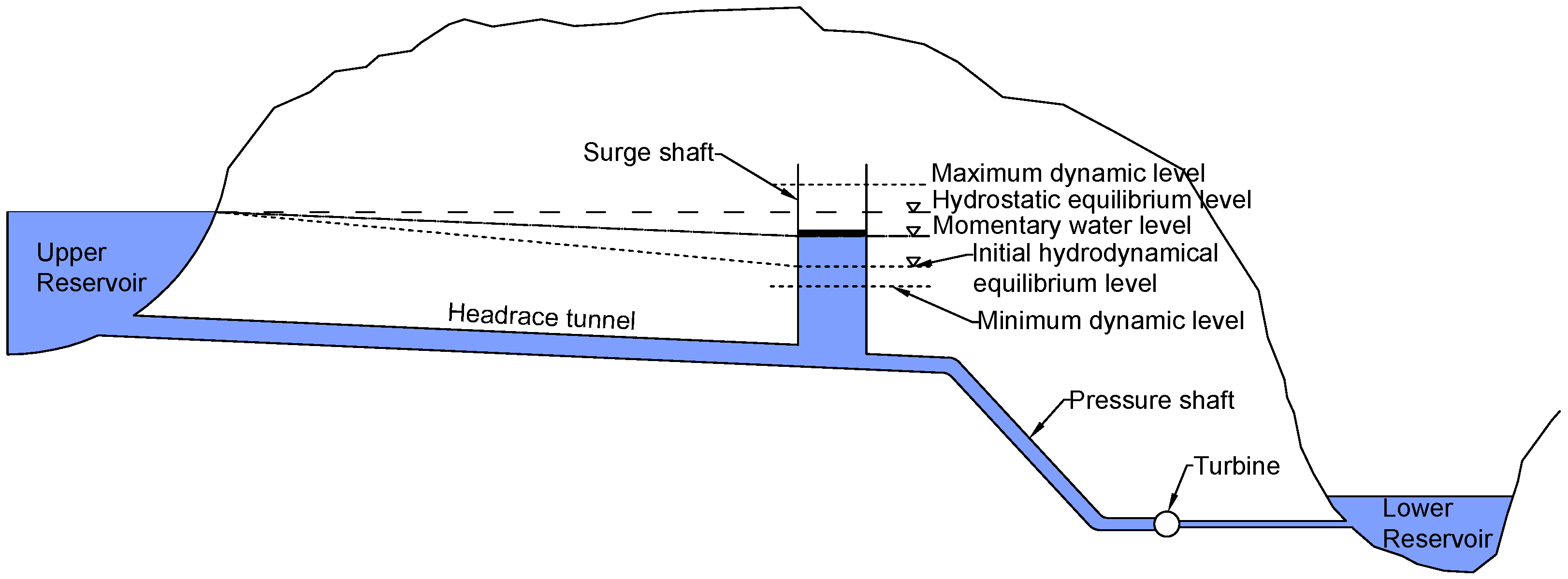
2. Hydraulic Transients in Hydropower Plants

During load changes, starts and stops in hydropower plants, there are fluctuations in water flow and pressure referred to as hydraulic transients [13]. For minimizing the detrimental effect of hydraulic transients, a surge tank/shaft may be provided in between the reservoir and the turbine. When measuring pressure in the tunnel between the surge tank and the turbine during a start, stop or load change, two superimposed pressure phenomena are observed—a water hammer with high frequency and mass oscillation with short frequency in synchronicity with the surge tank’s water level change [14]. The hydraulic transients originate at the turbine and travel through the penstock and unlined pressure tunnel. The hydraulic transients eventually diminish or decay due to steady and unsteady friction [15,16]. Figure 1 shows a simplified schematic of a waterway system with a surge tank.
The hydraulic transients can be separated into (1) the water hammer and (2) the mass oscillations. The time period of the mass oscillation in a frictionless pressure tunnel is expressed by Equation (1).
T = 2 π L A s g A t ,
where T is the time period of mass oscillation, L is the length of frictionless pressure tunnel, A t is the cross-sectional area of tunnel, A s is the cross-sectional area of surge tank, and g is the acceleration due to gravity. It is clear from Equation (1) that the time period of mass oscillation depends only upon the geometric characteristics of the pendulating system in the case of a frictionless pressure tunnel.
The time period of the water hammer is calculated as the length between the turbine and the surge tank divided by the water hammer’s celerity. A simplified approximate expression for the celerity of water hammer in rock tunnels was suggested by Parmakian 1963 [17] and is given by Equation (2).
c = 1 ρ 1 K + 1 G ,
where c is the pressure wave velocity, ρ is the density of water, K is the bulk modulus of elasticity of water, and G is the modulus of rigidity or shear modulus of rock. Field measurements in hydropower plants and unlined rock tunnels show that the water hammer’s celerity is often in the range of 1200–1400 m/s. As can be seen from Equations (1) and (2), the oscillation period of the water hammer is much faster than for mass oscillations. The relative amplitude of the mass oscillations compared with the water hammer is dependent on site-specific conditions. In some power plants, the water hammer is more severe, and in others the mass oscillations are most severe.

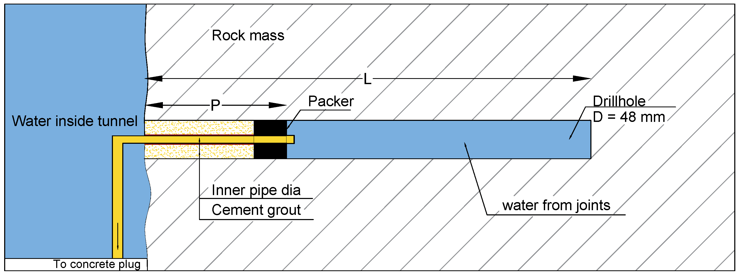
3. Fluid Flow in the Rock Mass

The flow of fluid in the rock mass primarily occurs through a network of fractures and joints since intact rock is close to impermeable. The void space geometry in the fractures and joints plays a significant role in the flow of fluid in the rock mass. Fluid flow through fractures and joints is mainly governed by properties such as aperture, roughness, contact area, mattedness, spatial correlation, tortuosity, channeling and stiffness [18]. According to Louis 1969 [19], the flow of water through the system of smooth joints with laminar flow follows a cubical law defined in Equation (3).
q = a 3 12 μ Δ p l ,
where q is the flow rate per width of joint, a is the aperture, Δ p is the pressure difference, l is the length of joint, and μ is the kinematic viscosity of fluid.
Fluid flow through joints is, in general, non-laminar and unevenly disturbed in the joints due to the roughness and infilling conditions of the joints [20]. The connectivity between joint systems in the rock mass, joint persistence, joint spacing and the infilling condition governs the permeability and extent of flow. A continuous and long persisting joint gives more flow in the tunnel. In general, the volumetric flow rate is lower in horizontal joints than the vertical ones [21]. When the compression strength of the joint wall is sufficiently high, even small shear movements can result in dilatancy, causing larger voids that allow water to flow more easily [22].

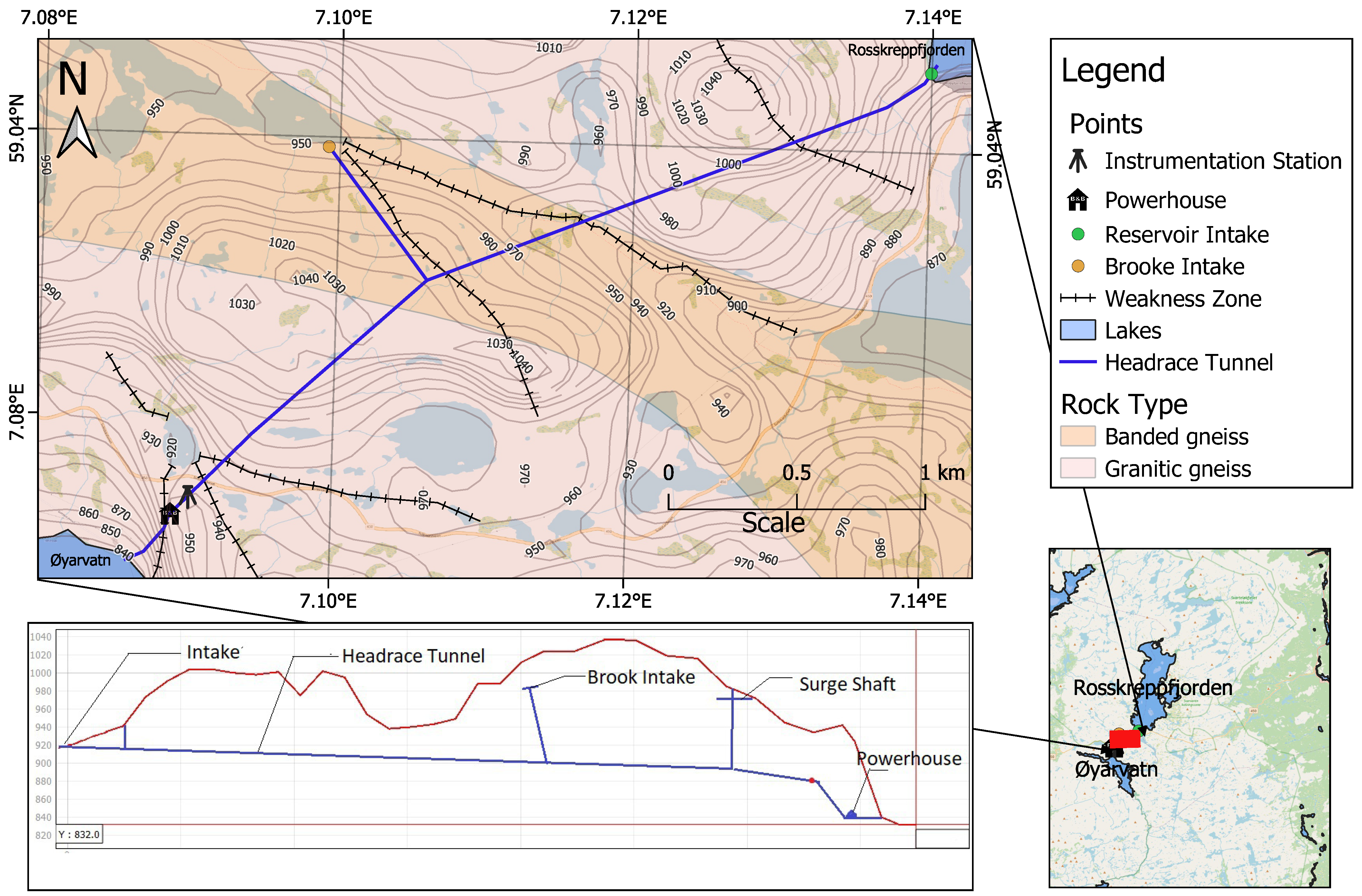
4. Case Study at Roskrepp Power Plant

Roskrepp hydropower plant, which came into operation in 1979, is located in Sirdal municipality in the southern part of Norway and is owned and operated by Sira-Kvina Kraftselskap. The power plant has a design discharge of 70 m3/s and an operating head that varies between 52 and 109 m owing to a large regulation height in the upper reservoir, Roskreppfjorden. The water from the main intake is conveyed via a 3500 m long, 7.5 m wide and 6.5 m high inverted D-shaped unlined headrace tunnel. The plant has an additional water inflow from a brook intake directly into the headrace tunnel. The power plant has an underground powerhouse and a vertical Francis unit with a rated power of 50 MW that produces an average annual energy of 105 GWh. The discharge from the turbines at the underground powerhouse is then released to Øyarvatn reservoir through a tailrace tunnel, which is again used by four cascading hydropower projects downstream before it flows into the sea at Åna-Sira. The general project layout of the project is shown in Figure 2.
The rock mass at the project area consists of course-grained banded gneiss and weakly schistose granitic gneiss. The engineering geological surface mapping shows that the general orientation of the foliation joints is in the range N 135°–150° E/40°–60° NE (Jf). In addition, two major cross-joint sets with strike/dip N 080°–100° E/70°–80° N (J1) and N 000°–020° E/ 40°–50° SE (J2) are present in the rock mass [23].
The instrumentation location is positioned downstream of the surge shaft and upstream of the turbine, where significant pressure changes occur during transients. For the measurement of pore pressure inside the rock mass, five boreholes with a diameter of 48 mm are drilled inside the rock mass near the intersection from the headrace tunnel to the access tunnel (Figure 3). The boreholes are sealed with packers and steel pipes are connected from inside of the packers, going through the water tunnel, and exiting through the concrete plug. At the dry side of the concrete plug, pressure transducers are connected to the steel pipes, effectively measuring the water pressure on the inside of the packers in the boreholes. GE Unik 5000 absolute pressure transducers are used with 0.2% of full-scale accuracy. One of the steel pipes is only connected to the water inside the headrace tunnel, and pressure transducer is installed for measuring the water pressure inside the main tunnel.
Inside each borehole, a stainless steel pipe with a 10 mm internal diameter is fixed using rubber packers as shown in Figure 3. The empty length of the borehole inside the rubber packer is used to investigate water pressure in the rock mass which is recorded in the pressure transducers located outside of the concrete plug and is connected through the stainless steel pipes. The tightened packer secures the steel pipe firmly within the boreholes, creating a hydraulic barrier between the pore pressure in the rock mass and the water pressure in the tunnel. In addition, the hole is cement-grouted between the packer and tunnel wall to make sure that there is no hydraulic connection between the tunnel water and the borehole beyond the packer (Figure 3). The packer is positioned at various distances from the tunnel wall inside the boreholes of varying lengths to study the borehole pressure responses with respect to distance from the tunnel wall. The information on packer length and effective length for hydraulic connection is given in Table 1.
Figure 4 shows the joint condition and borehole orientation at the instrumentation location (left) and the stereographic projection of the jointing condition at the instrumentation area (right). Table 2 provides information about the joint characteristic at the instrumentation location.

5. Analysis

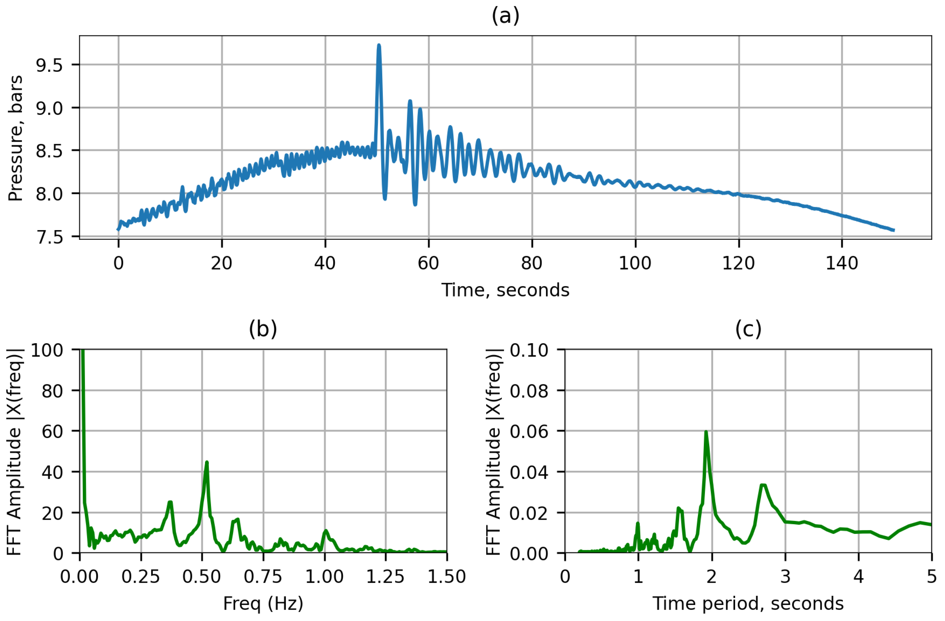
5.1. Finding Pressure Peaks in the Data

The pressure transducers measure water pressure in the tunnel and inside the rock through five boreholes. The data are recorded at a frequency of 10 Hz. This sampling frequency is high enough to record the high-frequency water hammer waves. Later in the analysis, it becomes evident that this sampling frequency effectively captures the water hammer waves. Alternatively, the Nyquist criterion can also be used for data acquisition, which says that the sampling frequency should be at least twice the frequency of the wave being sampled to properly reconstruct the original signal [24]. In total, for all the pressure transducers, there are 60 data points per second and millions of data points over the span of 5 years from 2018 to 2023. Handling such a large dataset can be difficult and time-consuming, involving tasks like accessing, retrieving, saving, analyzing, and interpreting the data. The raw dataset for water pressure of the tunnel and boreholes of May 2021 is shown in Figure 5a as an example.
To make this process more manageable, it was necessary to extract the useful data series from this extensive dataset. The useful data series refers to the sections where start and stop sequences are present or where pressure transients occur. An example of such extraction is shown in Figure 5b. These pressure peaks are not consistent and vary depending on factors like valve closure time, initial pressure, and load changes [25].
To efficiently analyze the data, it is essential to detect these pressure peaks and filter them in. Nevertheless, this task presents challenges due to the presence of noise in the pressure signal. To overcome this, a peak finding algorithm called “scipy.signal.find_peaks” was implemented in Python environment.
The direct use of the find_peaks function with raw data did not detect the peaks correctly due to the presence of noise. To address this, a continuous wavelet transformation (CWT)-based peak detection algorithm was used first but this approach took longer computational time. Hence, the Butterworth filter that offers smoother signals with a faster computational time, which according to Pröll 2023 [26] simplifies peak detection was used. The noise was filtered out using a low pass fourth-order Butterworth filter with a cutoff frequency of 0.005 Hz (time period of 200 s), which resulted in data with a smooth signal.
The smooth signal was then used to find the peaks using the find_peaks function. The function has multiple arguments, out of which prominence and width were used in the analysis. “Prominence” represents the minimum height of a peak relative to the lowest point in the waveform, while “width” indicates the minimum distance between two peaks. A hit and trial approach along with assistance from data visualization helped to determine the appropriate values and ensured effective peak detection. Finally, a prominence of 0.7 bar and a width of 200 s were found optimal to detect the upsurge peak of mass oscillation.
When there is a start sequence, the water is intermittently supplied by surge tanks, consequently resulting in a downsurge peak of the mass oscillations in the surge tank. The maximum drop in tunnel water pressure was identified by inversing the data in the find_peaks function.
To process the raw signal, a fourth-order Butterworth filter with a cutoff frequency of 0.0055 Hz was applied followed by the implementation of the find_peaks function. By setting a prominence value of 0.8 Hz and a width of 160 s, it was possible to identify nearly all the downsurge peaks throughout the entire study period. After the peaks were known, the waveform of tunnel water and borehole pressures around the peaks were extracted for further analysis.

5.2. Natural Frequency of Oscillation

At the instrumentation location, two waves viz. mass oscillation and water hammer can be observed. These oscillating waves cannot be measured separately because one wave superimposes with the other as they occur simultaneously. So, it is necessary to differentiate these waves to interpret and analyze them separately.
Fast Fourier Transformation (FFT) is an algorithm that converts a signal from the time domain to the frequency domain which can be used to find the natural or pure frequency of vibration [27]. A fully developed waveform of tunnel water pressure in a stop sequence was selected to find out the frequency of mass oscillation (Figure 6a). When the signal is transformed from the time domain to the frequency domain, it shows the constituent frequencies that make up the signal. In Figure 6b, it is evident that there are two major constituent frequencies of 0.004 Hz and 0.01 Hz. These frequencies correspond to the time period of 3.75 min and 1.54 min (Figure 6c).
As it can be seen in Figure 6c, the wave with a higher time period, i.e., 3.75 min as the oscillation between the reservoir and the surge shaft and a second oscillation with a period 1.54 min, is the wave oscillating between the reservoir and the brook intake. Note that the time period depends on the distance between the free water surfaces in the waterway system. If the distance between the free water surfaces is greater, the moving waves will have a longer time period and vice versa.
The same analysis using FFT on all the start and stop sequences throughout the study was performed. The results consistently showed a natural frequency of oscillation corresponding to a time period of 3.75 min throughout the study period. For this analysis, the tunnel water pressure data are considered because the borehole data do not provide information about the frequency of actual pressure surge waves occurring in the tunnel. This consistency in natural frequency shows that the time period of mass oscillation remains unchanged regardless of the discharge amount, reservoir level and start or stop sequences. According to Mosonyi 1991 [28], it is solely the function of geometric characteristics of the pendulating system and frictional resistance of the headrace tunnel.
It was found that FFT was able to decompose waves into their constituent frequencies that make up the signal of mass oscillation. However, it could not reveal the frequency of the water hammer when the pressure wave in Figure 6a was analyzed. At first, a simple theoretical approach was used to find out the frequency of the water hammer. For this, a theoretical water hammer frequency was calculated using Equation (2) which depends upon the modulus of rigidity (shear modulus) of the rock mass. The average shear modulus of 25 GPa was estimated using the elasticity modulus obtained from the laboratory test of intact rock samples [29]. With a distance of 87 m between the free water surface (surge shaft) and turbine, the wave velocity obtained from Equation (2) is 1391 m/s. This results in a theoretical water hammer frequency (f = c/2L) of 8 Hz. Frequencies higher than this are deemed to be generated by other structures, such as the vibration of the penstock.
One major limitation of FFT is that it captures total or overall information about frequency. That means that FFT analyzes the frequency that exists over the entire pressure signal. If we consider the full wave that includes mass oscillation, the effect of the water hammer is barely noticeable because there are other superimposed waves that make the water hammer wave difficult to detect. The water hammer dies out after 1–2 cycles of oscillating waves; hence, it is highly localized in time. Therefore, it was necessary to separate and isolate the oscillating wave associated with the water hammer for FFT analysis to effectively detect the water hammer. Figure 7a shows the extracted water hammer waves considered for FFT analysis.
It is evident from the time-domain graph in Figure 7c that the highest amplitude is obtained at a time period of 2 s. This time period corresponds to the water hammer in the system. Other pressure oscillations with small and large frequencies are also observed because of pipe vibration and different parts of the water hammer reflected by various physical structures and transitions between sensor location and turbine. However, the waves generated by reflection from structures would only be recorded if the measurements were taken close to the turbine. So, the major source of these high-frequency signals in the measurements is predominantly due to pipe vibration. This argument is supported by the fact that when the main inlet valve (MIV) is completely closed, signals with frequencies higher than 1 Hz decrease significantly. Closing the MIV stops the water flow toward the turbines, resulting in minimal vibrations in the pipes. It is evident that there are no significant waves of natural frequencies having a time period of less than 1 s (Figure 7c). The small amplitude rise at 1 s in Figure 7c indicates that the frequency corresponding to 1 s, i.e., 1 Hz, can be used to filter unnecessary noise for calculating total impact. This cutoff frequency of 1 Hz is lower than the frequency obtained from the theoretical approach using analytical formula.

5.3. Shutdown Procedure and Duration

In hydropower plants, there are two shutdown methods: emergency shutdown, which is sudden and can cause pressure fluctuations, and normal shutdown, a gradual process to reduce stress on electromechanical component [7]. Both shutdown methods involve two stages: first, partially closing the vanes to reduce flow, and second, fully closing the MIV, creating high pressure peaks (Figure 8a).
Determining the shutdown duration presents a challenge as the closure maneuver of the valve cannot be solely obtained from the pressure transient curve. For precise shutdown timing, it is essential to account for valve properties, including discharge coefficient, area, and closing procedure, which were unavailable. Although there may exist certain uncertainties that hinder the precision of obtaining the shutdown time, a relative measure of the shutdown speed is established in the analysis. This measure is derived from the time elapsed between the initiation of the shutdown event and the occurrence of the highest amplitude of mass oscillation after noise reduction, as depicted in Figure 8a. This relative measure is referred to as the “shutdown duration”. This approach was also used by Neupane et al. 2021 [7].
Figure 8b illustrates the shutdown duration trends from the start of the instrumentation until January 2023. Notably, there was a significant reduction in shutdown duration, dropping from approximately 120 s to around 60 s in late 2019. This change has provided a unique opportunity to explore the relationship between shutdown duration and its impact on the surrounding rock mass during transients. Here, shutdown durations of less than 75 s are classified as fast shutdowns, while durations exceeding 100 s are classified as slow shutdowns.

5.4. Quantifying the Hydraulic Impact

When plotting a transient event in the waterway system, it becomes evident that there is a delay in the pore pressure response within the rock mass compared to the tunnel. The delay in pore water pressure in the rock mass occurs due to a lag in the development of pore water pressure within the joints in the rock mass, since the flow of water is influenced by factors such as joint location, roughness, opening, length and connectivity between the joint system and available dynamic water pressure in the tunnel itself.
The presence of higher pore water pressure in the rock mass compared to the tunnel water pressure poses an impact on the surrounding rock mass adjacent to the tunnel wall. This is primarily due to the stress exerted by the surrounding rock mass towards the tunnel, which is predominantly destabilizing in nature against the resistance capacity of rock joints. Figure 9 illustrates the two situations for an arbitrary rock joint wall, and shows that when the pore pressure on the joint is higher than tunnel water pressure, it forces the block to move towards the tunnel. On the other hand, when tunnel water pressure is higher than pore water pressure in the rock mass, the same rock block is pushed inward to the rock mass. Such repeated cycles cause further loosening of the rock block. This unfavorable condition will be very common in hydropower plants with unlined tunnel systems and frequent changes in the operation regime.
In order to assess the impact of transients on the surrounding rock mass of a tunnel and establish an objective measure, a quantification method is necessary. Given that a situation where pore water pressure in the joint walls exceeds tunnel water pressure, it becomes essential to express this condition in numerical terms. This additional stress condition, referred to as “hydraulic impact” (HI), was first defined by Neupane et al. 2021 [7] and is measured in MPa·s. HI can be compared to dynamic viscosity or the force exerted on the joint surfaces per unit area integrated over time. The mathematical expression used for obtaining HI is expressed in Equation (4).
H I = t 1 t 2 ( B H P T W P ) d t , T W P < B H P 0 T W P B H P
where B H P is pore water pressure in the rock mass (borehole pressure), T W P is tunnel water pressure, and t 1 and t 2 are time intervals.
A typical shutdown event of May 2021, plotted in Figure 10, shows that boreholes 2 and 4 experience the hydraulic impact due to pressure lag between the tunnel and rock mass. At some instances after the valve closure, the pressure in the borehole is larger than the tunnel water pressure, which is unfavorable for tunnel walls. This unfavorable situation persists until three complete mass oscillations for borehole 2 and two complete mass oscillations for borehole 4 (Figure 10).
In contrast, BH1 and BH5 exhibit no phase lag between tunnel pressure and pore water pressure in the borehole, suggesting a lower risk to stability compared to the other three boreholes. This is due to the smaller pressure difference between the tunnel and boreholes. The pressure in BH3 is unaffected by the transient and the pressure is way below the tunnel water pressure. So, BH3 does not induce any HI on the tunnel walls.
This paper introduces a new quantification term called “maximum pressure difference” (MPD) for quantifying the impact of transients in the rock mass surrounding the unlined tunnel. It refers to the largest difference in pressure between tunnel water and rock joints during a transient event when the borehole pressure exceeds the tunnel water pressure. It is the force exerted per unit area on the joint surface and is measured in MPa or bars. It does not take account of the time of action of stress but only accounts for the magnitude of stress induced due to hydraulic transients. The rationale is that the maximum force will determine if the cyclic load is in an elastic or plastic regime, i.e., resulting in permanent deformation or not. So, for one transient event, there is one value of MPD expressed by Equation (5). The schematic representation of HI and MPD is shown in Figure 10.
M P D = m a x { B H P T W P } , T W P < B H P 0 T W P B H P

5.5. Method of Calculating HI and MPD

The raw data contain a significant amount of noise at higher frequencies. The first step involved removing these noises to ensure a noise-free signal. Subsequently, the waves generated by the water hammer and mass oscillation were separated. The design guidelines of the unlined pressure tunnel provide the FoS for mass oscillation and water hammer separately [11]. So, it was worthwhile to separate them to assess the impact of each component individually. The natural frequency of vibration is already calculated using FFT as described in Section 5.2. With this knowledge, a Butterworth low-pass filter is used to filter out waves with frequencies lower than the cutoff frequency. Figure 7 shows that the water hammer frequency with the largest amplitude in the frequency domain is 0.5 Hz, which corresponds to 2 s. Another peak is observed at 1 s. As explained in Section 5.2, the frequency corresponding to 1 s is adopted as the cutoff frequency for noise filtration. After applying Equations (4) and (5), the noise-filtered signal enabled the calculation of the total HI and MPD.
To determine the HI and MPD specifically due to mass oscillation, it is necessary to remove the water hammer waves from the signal as well. The frequency domain analysis revealed that the maximum amplitude of mass oscillation waves is 0.004 Hz, corresponding to 3.75 min, as depicted in Figure 7. Additionally, smaller amplitudes up to 0.015 Hz are also present. Hence, a cutoff frequency of 0.0167 Hz, corresponding to a time period of 1 min, was selected to filter out the water hammer waves from the overall signal. The subsequent calculation involved determining the area and magnitude between pressure pulses after applying this filter, which provided the HI and MPD values for mass oscillation, respectively. Finally, by subtracting the HI and MPD values obtained for mass oscillation from the total HI and MPD, the corresponding values for the water hammer were calculated. The cutoff frequencies for obtaining impacts due to various components of the waveform are shown in Figure 11. Figure 12 shows the overall formulated methodology for data analysis.

6. Results

The results are derived by observing pore pressure response over the years, specifically in the context of HI and MPD generation, analyzed through joint characteristics mentioned in Table 2. It subsequently elaborates on the induction of HI and MPD during start and stop sequences, and further analyzes the impact of shutdown duration on HI and MPD.

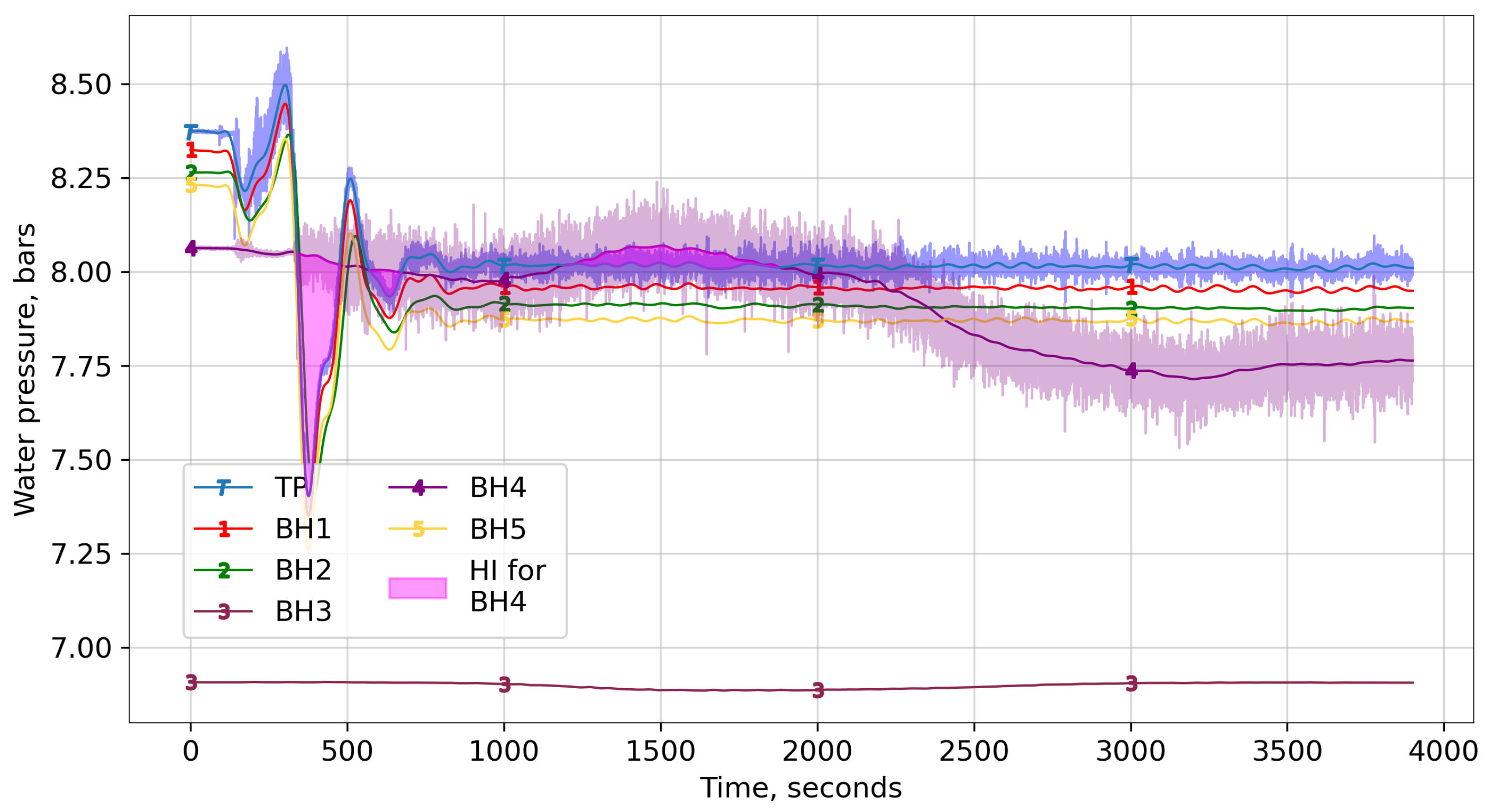
6.1. Pore Pressure Response

In this section, an overview of pore water pressure characteristics in relation to tunnel water pressure is discussed. The expected response to transients and pore water pressure behavior on the boreholes throughout the study period is evaluated. In addition, explanations are made of how the behavior of the boreholes can be related to HI and MPD.
Borehole 1 (BH1): BH1 intersects through approximately five foliation joints (Jf). BH1 also passes through Jfconductive, a conductive joint with a larger aperture giving continuous flow. Jfconductive intersects with BH1 at approximately 1.5 m from the tunnel wall (Figure 4).
Initially, BH1 exhibited responsiveness, particularly during shutdowns, as shown in Figure 13. However, from August 2018 until mid-November 2018, it stopped being responsive. After that period, it resumed being responsive. During shutdowns, BH1 has more water hammer pulses compared to other boreholes, resulting in the highest MPD, as depicted in Figure 14. However, the phase lag is minimal on this hole, almost similar to tunnel pressure.
Borehole 2 (BH2): BH2 intersects with cross-joint J1, which runs subparallel to foliation joint Jf (Figure 4). There is no hydraulic connection between BH2 and cross-joint J2, which is partially open in character. Cross joint J1, on the other hand, is a tight joint filled with impermeable clay (Table 1). Therefore, it was anticipated that BH2 may not exhibit significant response to the transients.
After over a year of instrumentation, BH2 gradually started becoming moderately responsive in December 2018 (Figure 13). Following the dewatering of the tunnel in May 2019 and its subsequent filling in September 2019, the behavior of BH2 changed, and it transformed into a moderately responsive joint. Over time, its responsiveness increased. By the end of August 2020, BH2 became more responsive compared to BH4, particularly during the start sequence. Figure 15 shows a typical response of BH2 during the stop sequence with its HI along with other boreholes.
During the inspection carried out one year after setting up the instrumentation station, it was discovered that the pipe connected to BH2 was broken. Efforts were made to fix the pipe and minimize its vibration by grouting. However, the pipe could not be fully repaired as it continued to induce HI even after maintenance. The broken pipe acted as a dummy or artificial joint since it was not fully connected to the tunnel water pressure, yet it still caused HI. Despite the breakage of the pipe connecting BH2, it can potentially be utilized to investigate the effects of variables like shutdown duration and static head on HI and MPD. Including BH2 in the analysis would not reveal the actual condition of the borehole, but rather help to describe the general behavior of a moderately responsive joint.
Borehole 3 (BH3): BH3 intersects with approximately four to five foliation joints (Jf), which are tight joints filled with clay. There is no hydraulic connection between BH3 and Jfconductive. Moreover, BH3 runs subparallel to J1. Therefore, it is expected that BH3 would not exhibit any response to the transients. BH3 has been a non-responsive joint since the beginning of the instrumentation program. It shows little to no response to the transients and does not induce any HI or MPD. However, the pressure of BH3 became higher than tunnel water in some instances following the start sequence in September and October 2019. The reservoir operation level started decreasing but the BH3, being a non-responsive joint, did not respond quickly to the reservoir and tunnel water level. Following the start sequence, the tunnel water level decreased steeply below the pressure of BH3, which induced HI and MPD in such a situation. The HI and MPD resulting from this situation can be observed in the start sequence depicted in Figure 13 and Figure 14, respectively.
Borehole 4 (BH4): BH4 intersects with approximately four to five J1s, which are tight joints filled with clay. BH4 also crosses with J2, which is a partly open joint with a washed-out infilling. The intersection point between J2 and BH4 is located approximately 8 m from the tunnel wall.
BH4 has shown moderately responsive behavior. The extent of responsiveness started decreasing in late December 2020 and again became normal in late January 2021. It induces more HI in the start sequence than in the stop sequence. Figure 15 shows the HI caused by BH4 in the start sequence enclosed by a large area between BH4 and tunnel water pressure. On some occasions, it causes HI even after 20 min of the start event (Figure 16). In February 2022, the characteristics of BH4 changed, making it unable to induce HI significantly, especially in the stop sequence, as indicated by the flat lines in the cumulative plots in Figure 13 and Figure 14 (right).
Borehole 5 (BH5): BH5 is on the left side of the tunnel wall and passes only through Jf which is a tight joint (Figure 4 and Table 2). So, it is expected to be a non-responsive borehole. However, the effective length of this borehole is 8 m, so it could be more responsive than BH3, which has an effective length of 5m.
BH5 started becoming a highly responsive borehole from March 2020 and onward, but did not induce HI or MPD because it follows the tunnel water pressure without phase lag. Lately, the characteristics of BH5 can be classified as a highly responsive joint that follows tunnel water pressure without generating HI or MPD.

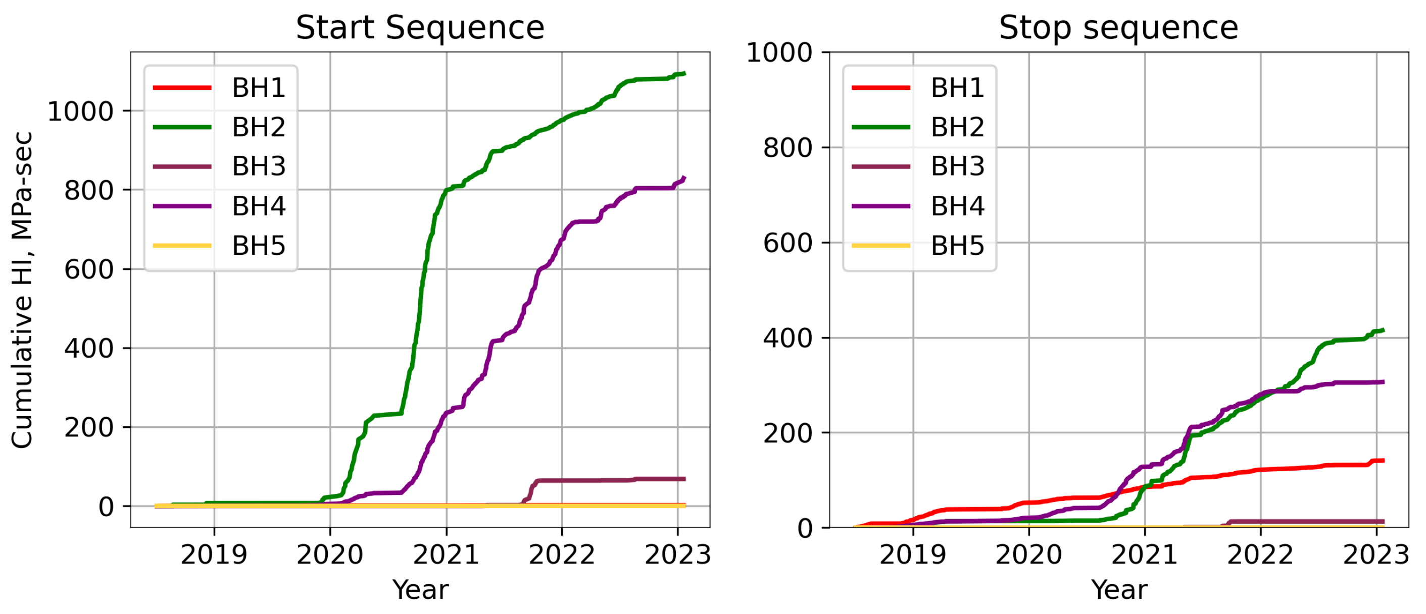
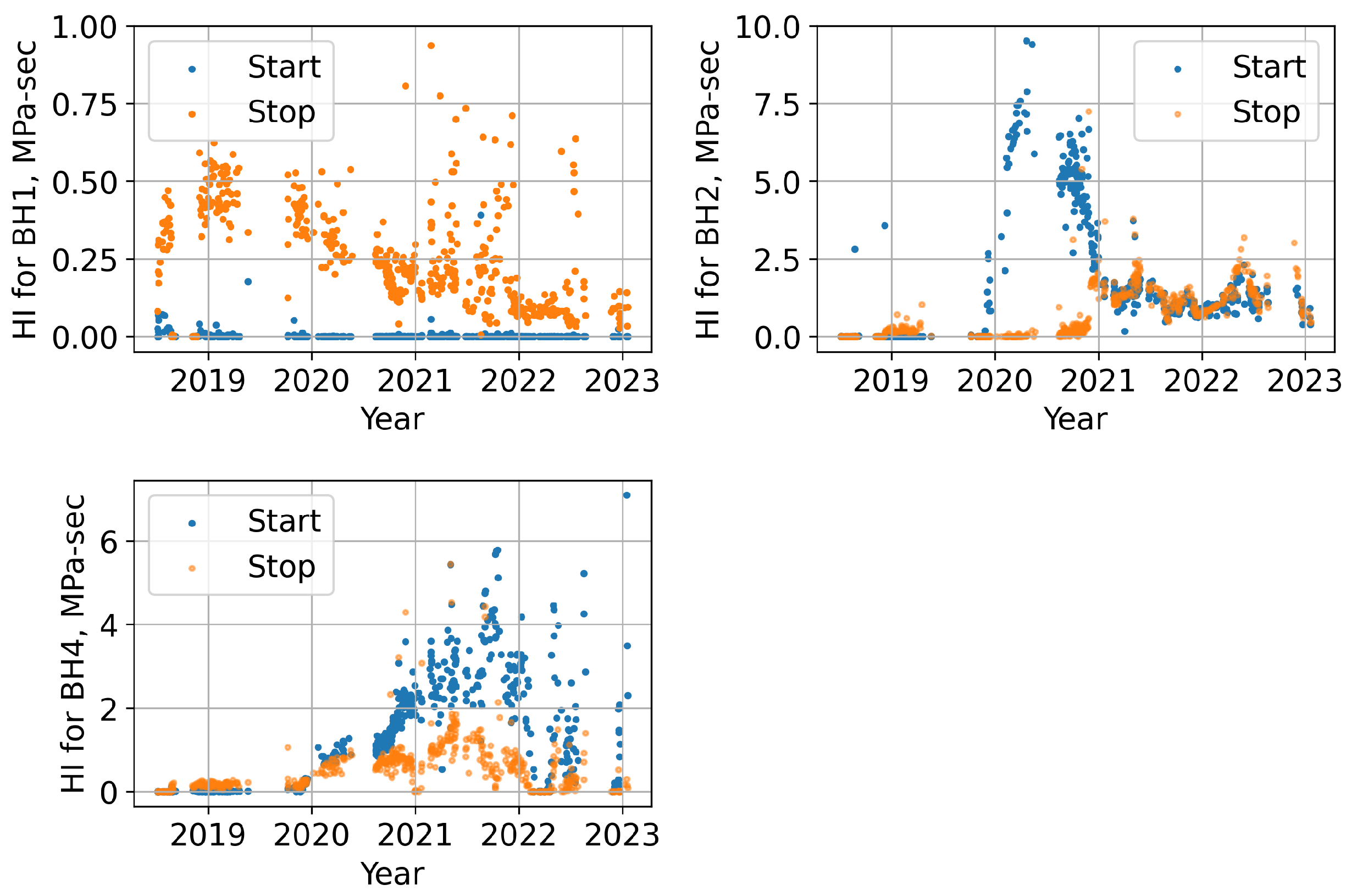
6.2. Start and Stop Sequence

A previous study predominantly focused on analyzing the stop sequence while giving less attention to the start sequence [12]. This omission was due to the presence of a considerable amount of noise in the measurement data of the start sequence and constraints in the available time, which made it challenging to cover.
Upon analyzing the HI and MPD for the boreholes, it was observed that the start sequence imposes higher stress on rock joints compared to the stop sequence. More importantly, throughout the study period comprising 1008 start and stop sequences, the HI values were on average 2.97 times higher for BH2 and 3.05 times higher for BH4 in start sequences than in stop sequences. These findings suggest that the start sequence generates approximately three times more HI than the stop sequence, which is significant in terms of HI in unlined pressure tunnels due to transients. The cumulative values of HI and MPD in Figure 13 and Figure 14 show that BH2 and BH4 exhibit greater HI during start sequences compared to stop sequences. On the other hand, BH1 exhibits higher MPD during stop sequences because the impact induced by the water hammer is relatively greater than that by mass oscillation.
The start and stop sequences are two different events that occur one after the other. During the stop sequence, water cannot enter the penstock and instead moves towards the surge shaft, causing an increase in water level and pressure in the tunnel. The borehole pressure follows the tunnel water pressure but with a slight delay and a reduced peak. As the water level drops in the surge shaft after reaching its maximum, the borehole pressure still follows the tunnel water pressure but with a lag, and the pressure in the borehole becomes higher than the tunnel water pressure, resulting in HI as indicated in Figure 15.
On the other hand, during the start sequence, water is intermittently supplied to the turbine from the surge shaft, leading to a sudden decrease in water level and tunnel water pressure. So, naturally, the first series of oscillations is a downsurge. The boreholes also follow the tunnel water pressure but with a delay (time lag), and their pressure becomes higher than the tunnel water pressure. This situation also imposes a destabilizing force acting inward in the joint wall with a direction towards the tunnel. In certain situations of stop sequences, the pressure in the borehole remains higher than the tunnel pressure even after the water level in the tunnel stabilizes (Figure 16), where one can see that BH4 induces HI even 20 min after the start of turbines. The HI for all start and stop events over the study period is shown in illustrations. BH4 induces HI even 20 min after the start of the turbines. Therefore, the HI induced during the start sequence is observed higher as compared to the stop sequence. The HI for all start and stop events over the study period is shown in Figure 17.

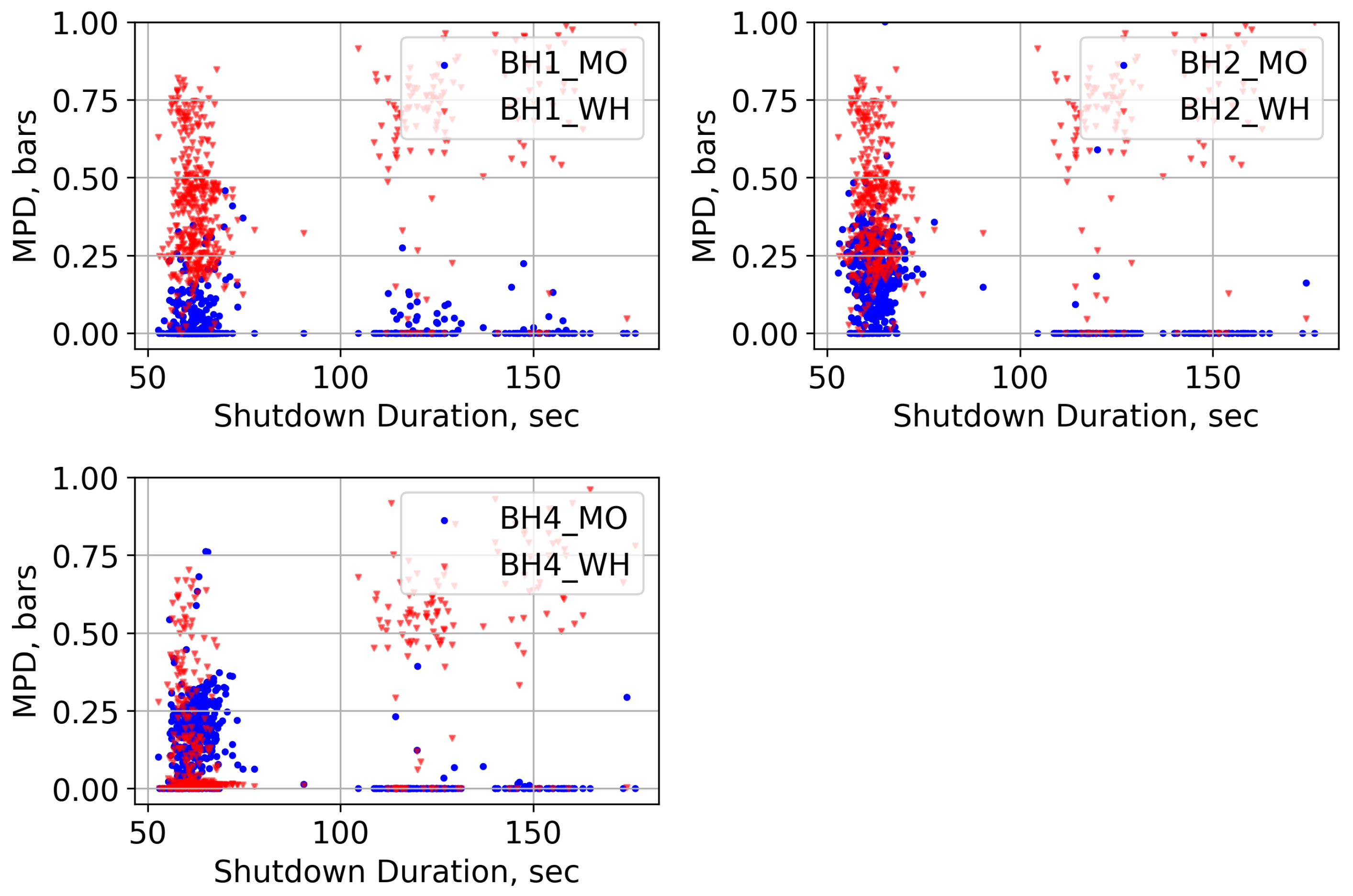
6.3. Effect of Shutdown Duration

The shutdown duration can have an influential effect on the transients in the waterway system of hydropower plants [30]. The shutdown duration can also have an effect on the rock mass surrounding the tunnel [7]. Hence, it is necessary to understand the effect of shutdown duration on transients and the impact on the rock mass surrounding the tunnel.
The minimum and maximum shutdown duration in Roskrepp hydropower plant are 53 s and 177 s, respectively, with an average shutdown duration of 80 s. Figure 18 shows two shutdown events in January 2019 and March 2020. As seen in Figure 18, the faster shutdown duration of March 2020 has exhibited higher HI than in January 2019. It is noted here that the tunnel water pressure for both the 2019 and 2020 events is filtered with a cutoff frequency of 0.01167 Hz.
In the January 2019 transient, a gradual de-loading and shutdown process is observed, while the 2020 transient exhibits a faster shutdown prior to MIV closure. Despite having a similar range for MIV closure, the 2020 transient generates larger water hammer pulses, indicating a more rapid shutdown. Furthermore, the amplitude of mass oscillation is greater in the 2020 transient compared to the 2019 transient, with a peak being reached quickly. The faster shutdown results in a steeper curve for mass oscillation, leading to a larger time lag between the tunnel water pressure and the pore water pressure in the rock mass. It is highlighted here that the shutdown durations for January 2019 and March 2020 are 58 s and 155 s, respectively, while the MIV closure time is 145 s for both transients. The combination of a larger time lag and a greater amplitude during the shorter shutdown duration results in a larger HI.
Figure 19 shows the HI of 504 shutdown events in relation to shutdown duration recorded over the study period. As Figure 19 indicates, the HI for BH1 is primarily due to water hammer for both longer and shorter shutdown duration. The effect due to mass oscillation is almost negligible for BH1. The HI for BH1 is primarily due to the water hammer for both longer and shorter shutdown durations. The effect due to mass oscillation is almost negligible for BH1. Further, when the shutdown period is shorter, there is more phase lag between tunnel water and pore water pressure in BH2 and BH4 creating a situation where pore water pressure in the borehole is greater than water pressure in the tunnel for a longer duration. As HI is the pressure difference multiplied by time, HI becomes larger for mass oscillation due to a larger area of pressure difference. In the case of a longer shutdown period, the pressure amplitudes and steepness of surges are lower compared to shorter (faster) shutdown periods. This provides time for the pore water pressure in the boreholes to adjust with the tunnel water pressure as evident from the typical transient event of January 2019 (Figure 18).
In both shorter and longer shutdown periods, the water hammer component is still present in the waves that have higher frequencies. In both BH2 and BH4, this induces HI even during longer shutdowns but is not as strong as mass oscillation. In moderately responsive joints, HI is primarily caused by the water hammer for longer shutdown durations.
If we consider MPD with respect to shutdown duration to quantify the impact of transient, the scenario is different as compared to HI. It is seen that the effect of the water hammer is larger than mass oscillation in all boreholes irrespective of the shutdown duration as shown in Figure 20. MPD only measures the water pressure difference between boreholes and tunnels. MPD has two clusters for longer and shorter shutdown durations. The MPD ranges from 0.2 to 0.8 bars for shorter shutdowns and 0.6 to 1 bar for longer shutdowns.
Results from the relation of HI and MPD with shutdown durations suggest that the impact of transients due to the water hammer increases with a longer shutdown duration because a longer shutdown duration allows more pulsating waves before MIV closure. After MIV closure, the water hammer waves also create some time lag, which induces more pressure difference.
Figure 19 and Figure 20 show two clusters of shutdown durations around 60 s and 120 s. The average HI in these two shutdown durations shows that when the shutdown duration is decreased by half the HI may be as high as five times as given by BH2 (5.02 times) and BH4 (4.65 times).

7. Discussion

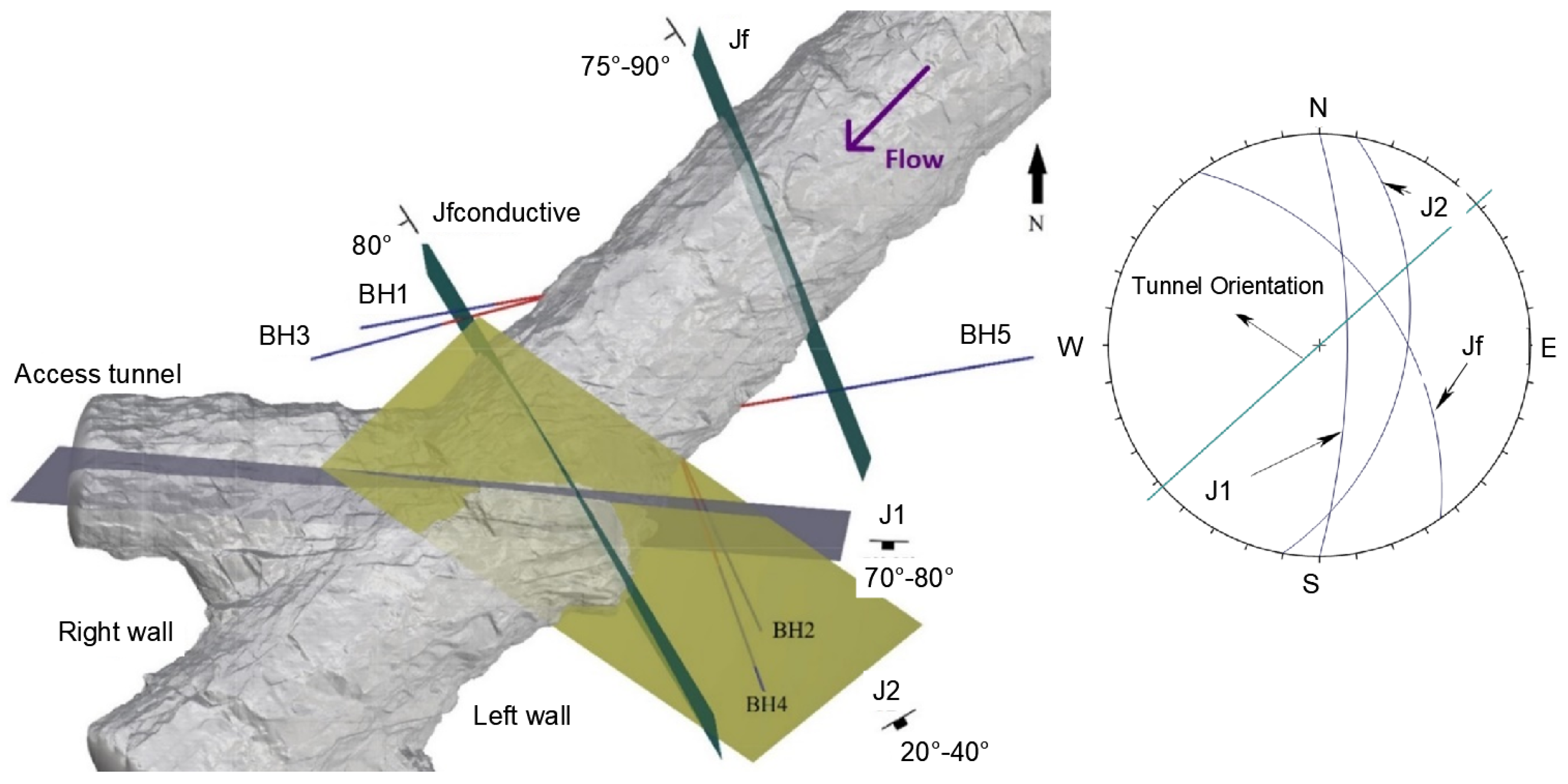
7.1. Joint Characteristics

Based on the water pressure data from boreholes, it was observed that BH1 and BH4 initially showed a responsive behavior with respect to tunnel water pressure during transients, while BH2, BH3, and BH5 showed nonresponsive behavior. The nonresponsive boreholes intersected joints Jf and J1, which have a narrow aperture with clay filling and a spacing of 1 m. On the other hand, BH1 intersected the conductive joint Jfconductive, while BH4 intersected J2. Jfconductive and J2 were found to have partially open joints with a washed-out filling (Table 2). It can be inferred that the responsive nature of the boreholes is influenced by Jfconductive and J2. The joints can be categorized based on their responsiveness, with conductive joints referring to those with large apertures (such as J2 and Jfconductive) that have a direct hydraulic connection to tunnel water pressure, and nonconductive joints referring to those with tight joints (J1 and Jf).
BH1 and BH4 show a response to the transients with a bit different behavior; however, they pass through joints having similar characteristics but at different lengths from the tunnel’s contour wall. BH1 intersects Jfconductive at 1.5 m and BH4 intersects J2 at 8 m from the tunnel wall. Therefore, it can be deduced that the difference in pore pressure response of boreholes intersecting similar joints is mainly due to the distance that a transient should travel inside the rock mass.
Additionally, it is important to note that the boreholes passing through these conductive joints induce HI and MPD. This suggests that the effect of mass oscillation and the water hammer can reach deep into the rock mass through the network of joints. This also highlights that the pore water pressure response of the rock mass is primarily controlled by the character of the joint system.

7.2. Behavior of Monitored Boreholes

The pore water response of boreholes behaves differently throughout the study period. BH1, BH3, and BH4 remained relatively stable throughout the study period, while BH2 and BH5 exhibited changes. Initially, both boreholes did not show response to transients, but over time, they became moderately responsive and highly responsive, respectively. Based on their response behavior or the boreholes after 2021, the responses can be classified into four different types, i.e., highly responsive, responsive, moderately responsive, and non-responsive. Schematic representation of the response of different types of boreholes during transients is shown in Figure 21 and information about the borehole type is listed in Table 3.
Highly responsive boreholes follow tunnel water pressure during transients and hence are unlikely to induce HI and MPD. Regarding responsive boreholes, BH1 induces HI and MPD during the water hammer with a time lag. BH1 lags tunnel water pressure especially during water hammer waves and less for mass oscillation. So, it induces HI especially due to the water hammer. As seen in Figure 17, BH1 does not include HI in the start sequence while it does in the stop sequence, suggesting that the water hammer component is weak in the start sequence. Moderately responsive boreholes (BH2 and BH4) include HI and MPD during both water hammer and mass oscillation, which indicates that these two boreholes have time lag both in mass oscillation and water hammer. Non-responsive boreholes show little to no response during transients and do not induce any HI and MPD.

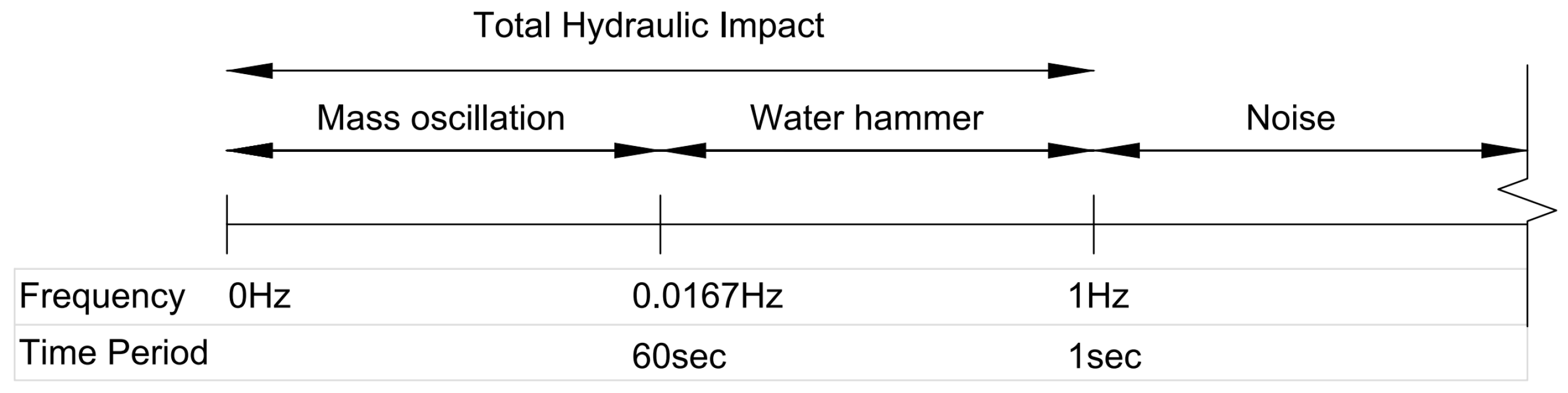
7.3. Natural, Cutoff and Sampling Frequency

In the analysis carried out by [7], three distinct frequencies of mass oscillations with 3.4, 1.6, and 1.1 min were observed, which represent oscillations between the reservoir and the surge shaft, between the reservoir and the brook intake, and between the brook intake and the surge shaft, respectively. However, this analysis has further identified a natural frequency of 3.7 and 1.54 min. But FFT analysis was unable to capture the natural frequency of mass oscillation between the brook intake and the surge shaft. The limited impact of the relatively small-sized brook intake on the mass oscillation may explain why the transducers could not record this specific wave frequency, which may be linked to time periods between the two studies and the order of filter used in the analysis.
Calculating the cutoff frequency for the water hammer based on theoretical approaches considering wave velocity and the length of the free water surface and turbine can lead to larger discrepancies. Therefore, a theoretical cutoff frequency of 8 Hz was obtained instead of a cutoff frequency of 3 Hz used by [7]. It is emphasized here that the FFT analysis provides detailed information on the natural frequency of pressure waves, and it is a practical approach to determine the cutoff frequency and separate signals based on frequency. Analyzing the waveform of the water hammer using FFT, we revealed that a cutoff frequency of 1Hz can effectively filter out noise and capture the total HI.
The sampling frequency for data acquisition from pressure transducers was fixed at 10 Hz. It was decided based on the time required by the wave to reflect from the instrumentation location to the turbine and back to the instrumentation location. The current high sampling frequency from the pressure transducer generates a large amount of data, making data handling and processing challenging. If long-term data storage is required, the sampling frequency can be reduced theoretically to 2 Hz (0.5 s). This frequency is obtained by doubling the maximum frequency of the water hammer, i.e., 1 Hz. However, due to the presence of noise, it is recommended to keep it at 5 Hz. This ensures quality of the data and at the same time increases the storage duration of pressure data.

7.4. Design Practice

The existing principles for the design of an unlined pressure tunnel protect only against hydraulic jacking, while the possibility of a block falls due to operational factors, which has not been addressed by the existing design criteria. There could be instances of unnoticed intact rock bridges during tunnel construction that may weaken over time due to cyclic loading and cumulative HI and MPD. This can exceed the fatigue strength of the intact rock bridge, leading to its rupture and subsequent block falls in tunnel. A similar study conducted by Preisig et al. 2016 [31] focused on the hydromechanical fatigue of intact rock bridges in deep-seated landslides. The primary cause of this fatigue was identified as the changes in pore water pressure caused by transients. Neupane et al. 2021 [9] also demonstrated the formation and failure of intact rock bridges on surrounding rock mass leading to rock blockage failure. These lessons are important in tunnels excavated through schistose rock formations such as phyllite and schist, especially in areas where there is a risk of future block falls due to damage to the intact rock bridges and the presence of partially open and conductive joints.
This signifies that the long-term stability of pressure tunnels against instabilities caused by pressure transients must be considered in the design, taking into consideration of the start/stop sequence and shutdown duration. The start sequence induces more HI and MPD, while the shutdown duration is a key parameter that affects HI and MPD.

7.5. Operational Requirements

Hydropeaking refers to the rapid changes in hydropower production that occur in response to fluctuations in electricity generation and demand of the electricity market. Hydropeaking is hence related to the start and stop sequence in hydropower operations. To safeguard the environment, certain restrictions are imposed on the change in amplitude of discharge, rate of change in water level, and frequency of discharge and water level changes during hydropeaking [32]. In some hydropower, there are also regulations for hydropeaking due to electromechanical constraints [9]. Coordinating factors with the start and stop sequence and shutdown duration may help minimize the hydraulic impact on tunnels, safeguard electromechanical equipment and protect the environment at the same time, all through a cohesive effort. This approach creates a win–win situation for all factors considered.

8. Conclusions and Recommendations

The analysis carried out on the hydraulic and pore water pressure data record monitored at Roskrepp hydropower plant over the period 2018 to 2023 provided a unique understanding of the effect of frequent start and stop sequences of unlined pressure tunnels of hydropower plants. The following conclusions are drawn from the framework developed to analyze data and quantify the impact caused by transients on the surrounding rock mass of unlined pressure tunnels.
  • The impact of the start sequences on the rock mass due to transient-induced cyclic loading is greater than the impact of the stop sequences. The analysis suggests that start sequences produce three times as much HI as the stop sequences in the operation of a hydropower plant under hydropeaking.
  • The analysis of pore pressure data reveals that the shutdown duration has a direct influence on HI. When the shutdown duration is reduced by half, the HI increases by five times.
  • The response of pore pressure in the rock joints is greatly influenced by the properties of joints like joint wall opening (aperture), roughness, infilling condition, joint spacing and persistence.
  • HI and MPD can be used as complementary values to quantify the impact of hydraulic transient in unlined pressure tunnels.
  • A water hammer can travel into a rock mass and cause a difference in the pressure inside the rock mass. So, it cannot be neglected in the design of unlined pressure tunnels since it will have long-term operational impacts.
Hence, it is recommended that hydropower owners start instrumentation programs to further enhance the knowledge of the link between HI and MPD with start–stop sequences and to understand transient induced instabilities in unlined pressure tunnels. It is noted here that when the difference in pressure between the tunnel and the joint walls changes, acting stresses also vary, which causes displacement leading to the increase in aperture, permeability and fluid flow. This causes the decrease in strength and stiffness of the rock joints. Hence, it is advisable to concurrently track borehole deformations alongside pressure measurements. The deformation data monitored would be helpful in examining the relationship of stress, displacement, dilation, and conductivity in joints. This approach could potentially serve as validation for the numerical model [33] relating to the hydro-mechanical coupling of joints. Such a study will help to find out the relationship between the behavior of rock mass and tunnel water pressure during transients, which will make it possible to predict the variations in HI and MPD.

Author Contributions

Conceptualization, S.G., K.K.P. and K.V.; analysis, S.G.; data investigation, S.G., resources, K.V. and K.K.P.; writing—original draft preparation, S.G.; writing—review and editing, K.K.P. and K.V.; visualization, S.G.; software, S.G.; supervision, K.K.P. All authors have read and agreed to the published version of the manuscript.

Funding

The work is funded through the HydroCen research centre. The funding from Sira-Kvina is included through HydroCen.

Data Availability Statement

Data cannot be shared due to confidentiality.

Acknowledgments

This research is the continuation of the research program “Norwegian Research Centre for Hydropower Technology (HydroCen)”. The authors would like to express their gratitude to Sira-Kvina kraftselskap for the cooperation and financial contribution in the instrumentation of headrace tunnel at Roskrepp Hydropower Plant. The authors also acknowledge the research carried out by Bibek Neupane who was involved in planning and installation of monitoring instrument.

Conflicts of Interest

The authors declare no conflict of interest.

References

  1. Panthi, K.K.; Basnet, C.B. State-of-the-art design guidelines in the use of unlined pressure tunnels/shafts for hydropower scheme. In Proceedings of the ISRM International Symposium—10th Asian Rock Mechanics Symposium, ARMS 2018, Singapore, 29 October–3 November 2018. [Google Scholar]
  2. Rancourt, A.J. Guidelines for Preliminary Design of Unlined Pressure Tunnels. Ph.D. Thesis, McGill University, Montreal, QC, Canada, 2010. [Google Scholar]
  3. Bye, T.; Hope, E. Deregulation of Electricity Markets: The Norwegian Experience. Econ. Political Wkly. 2005, 40, 5269–5278. [Google Scholar]
  4. Eurelectric. Hydro in Europe: Powering Renewables; Technical Report; Eurelectric: Brussels, Belgium, 2011. [Google Scholar]
  5. Skar, C.; Jaehnert, S.; Tomasgard, A.; Midthun, K.; Fodstad, M. Norway’s role as a flexibility provider in a renewable Europe. In A Position Paper Prepared by FME CenSES; CenSES Centre for Sustainable Energy Studies: Trondheim, Norway, 2018; Volume 80. [Google Scholar]
  6. Egging, R.; Tomasgard, A. Norway’s role in the European energy transition. Energy Strategy Rev. 2018, 20, 99–101. [Google Scholar] [CrossRef]
  7. Neupane, B.; Vereide, K.; Panthi, K.K. Operation of Norwegian hydropower plants and its effect on block fall events in unlined pressure tunnels and shafts. Water 2021, 13, 1567. [Google Scholar] [CrossRef]
  8. Bråtveit, K.; Bruland, A.; Brevik, O. Rock falls in selected Norwegian hydropower tunnels subjected to hydropeaking. Tunn. Undergr. Space Technol. 2016, 52, 202–207. [Google Scholar] [CrossRef]
  9. Neupane, B.; Panthi, K.K.; Vereide, K. Cyclic fatigue in unlined hydro tunnels caused by pressure transients. Int. J. Hydropower Dams 2021, 28, 46–54. [Google Scholar]
  10. Palmström, A.; Broch, E. The design of unlined hydropower tunnels and shafts: 100 years of Norwegian experience. Int. J. Hydropower Dams 2017, 24, 72–79. [Google Scholar]
  11. Benson, R.P. Design of unlined and lined pressure tunnels. Tunn. Undergr. Space Technol. Inc. Trenchless 1989, 4, 155–170. [Google Scholar] [CrossRef]
  12. Neupane, B. Long-Term Impact on Unlined Tunnels of Hydropower Plants Due to Frequent Start/Stop Sequences. Ph.D. Thesis, Norwegian University of Science and Technology, Trondheim, Norway, 2021. [Google Scholar]
  13. Chaudhry, H. Applied Hydraulic Transients Third Edition; Springer: Columbia, SC, USA, 2014. [Google Scholar]
  14. Jaeger, C. Present Trends in Surge Tank Design. Proc.-Mech. Eng. 1953, 168, 91–124. [Google Scholar] [CrossRef]
  15. Khilqa, S.S.E. Damping in Transient Pressurized Flows Damping in Transient Pressurized Flows. Ph.D. Thesis, University of South Carolina, Columbia, CS, USA, 2019. [Google Scholar]
  16. Vítkovský, J.P.; Bergant, A.; Simpson, A.R.; Lambert, M.F. Systematic Evaluation of One-Dimensional Unsteady Friction Models in Simple Pipelines. J. Hydraul. Eng. 2006, 132, 696–708. [Google Scholar] [CrossRef]
  17. Parmakian, J. Waterhammer Analysis; Dover Publications, Inc.: New York, NY, USA, 1963. [Google Scholar]
  18. Hakami, E. Aperture Distribution of Rock Fractures. Ph.D. Thesis, Royal Institute of Technology, Stockholm, Sweden, 1995. [Google Scholar]
  19. Louis, C. Study of Groundwater Flow in Jointed Rock and Its Influence on the Stability of Rock Masses; Imperial College of Science and Technology: London, UK, 1969; pp. 1–90. [Google Scholar]
  20. Panthi, K.K.; Basnet, C.B. Fluid Flow and Leakage Assessment Through an Unlined/Shotcrete Lined Pressure Tunnel: A Case from Nepal Himalaya. Rock Mech. Rock Eng. 2021, 54, 1687–1705. [Google Scholar] [CrossRef]
  21. Gudmundsson, A.; Berg, S.S.; Lyslo, K.B.; Skurtveit, E. Fracture networks and fluid transport in active fault zones. J. Struct. Geol. 2001, 23, 343–353. [Google Scholar] [CrossRef]
  22. Holmøy, K.H. Significance of Geological Parameters for Predicting Water Leakage in Hard Rock Tunnels. Ph.D. Thesis, Norwegian University of Science and Technology, Trondheim, Norway, 2008. [Google Scholar]
  23. Neupane, B.; Panthi, K.K.; Vereide, K. Effect of Power Plant Operation on Pore Pressure in Jointed Rock Mass of an Unlined Hydropower Tunnel: An Experimental Study. Rock Mech. Rock Eng. 2020, 53, 3073–3092. [Google Scholar] [CrossRef]
  24. Lévesque, L. Nyquist sampling theorem: Understanding the illusion of a spinning wheel captured with a video camera. Phys. Educ. 2014, 49, 697–705. [Google Scholar] [CrossRef]
  25. Guo, W.; Wang, B.; Yang, J.; Xue, Y. Optimal control of water level oscillations in surge tank of hydropower station with long headrace tunnel under combined operating conditions. Appl. Math. Model. 2017, 47, 260–275. [Google Scholar] [CrossRef]
  26. Pröll, Samuel. Finding Peaks in Noisy Signals (With Python and JavaScript). Available online: https://www.samproell.io/posts/signal/peak-finding-python-js/ (accessed on 20 March 2023).
  27. Lyons, R. Understanding Digital Signal Processing; Prentice Hall: Hoboken, NJ, USA, 2011. [Google Scholar]
  28. Mosonyi, E. High-Head Power Plants; Akadémiai Kiadó: Budapest, Hungary, 1991; Volume Two/A. [Google Scholar]
  29. Neupane, B.; Panthi, K.K. Evaluation on the Effect of Pressure Transients on Rock Joints in Unlined Hydropower Tunnels Using Numerical Simulation. Rock Mech. Rock Eng. 2021, 54, 2975–2994. [Google Scholar] [CrossRef]
  30. Bhattarai, K.P.; Zhou, J.; Palikhe, S.; Pandey, K.P.; Suwal, N. Numerical Modeling and Hydraulic Optimization of a Surge Tank Using Particle Swarm Optimization. Water 2019, 11, 715. [Google Scholar] [CrossRef]
  31. Preisig, G.; Eberhardt, E.; Smithyman, M.; Preh, A.; Bonzanigo, L. Hydromechanical rock mass fatigue in deep-seated landslides accompanying seasonal variations in pore pressures. Rock Mech. Rock Eng. 2016, 49, 2333–2351. [Google Scholar] [CrossRef]
  32. Bakken, T.H.; Harby, A.; Forseth, T.; Ugedal, O.; Sauterleute, J.F.; Halleraker, J.H.; Alfredsen, K. Classification of hydropeaking impacts on Atlantic salmon populations in regulated rivers. River Res. Appl. 2021, 39, 313–325. [Google Scholar] [CrossRef]
  33. Ki-Bok, M.; Rutqvist, J.; Tsang, C.F.; Jing, L. Stress-dependent permeability of fractured rock masses: A numerical study. Int. J. Rock Mech. Min. Sci. 2004, 41, 1191–1210. [Google Scholar] [CrossRef]
Figure 1. Schematic of a waterway system with surge tank and pressure levels during steady state and hydraulic transients.
Water 15 03894 g001
Figure 2. Map of Roskrepp hydropower plant and geological setting.
Water 15 03894 g002
Figure 3. Details of borehole with location of packer and connection of the steel pipes.
Water 15 03894 g003
Figure 4. Three-dimensional laser scanned isometric view showing the location of the borehole with respect to joints at instrumentation location (left). The blue portion represents the segment of the borehole between the packer and the end of the borehole where the pore water pressure is registered. The red segment is grouted with cement to hinder possible leakage. J2 is a random joint occurring at the instrumentation location. Modified from Neupane et al. 2020 [23]. Stereographic projection of joint sets at the instrumentation area (right).
Water 15 03894 g004
Figure 5. (a) Unprocessed dataset for May 2021. Note the prolonged linear sections, resulting from the absence of pressure fluctuations between peaks, necessitating increased data storage. (b) The refined May 2021 dataset, containing exclusively transient data. The time in the x-axis is the time period of extracted data and is not to be confused with the number of seconds in a month.
Water 15 03894 g005
Figure 6. Results of FFT analysis applied in mass oscillation. (a) The surge wave considered for analysis; here, only the one-half cycle of the oscillating wave is taken. (b) The results of FFT in frequency domain. (c) The same result in time domain.
Water 15 03894 g006
Figure 7. Results of FFT analysis applied only in water hammer surge wave. (a) The surge wave considered for analysis, here only the one-half cycle of the oscillating wave is taken. (b) The results of FFT in the frequency domain. (c) The same results in time domain.
Water 15 03894 g007
Figure 8. (a) Shutdown duration and the initial pressure head (water head) in a stop transient event. Faint blue shows the raw data with noise and the blue line shows filtered data with a cutoff frequency of 0.0167 Hz. (b) Shutdown duration over the years.
Water 15 03894 g008
Figure 9. Schematic illustration of favorable and unfavorable situations for block falls during hydraulic transients.
Water 15 03894 g009
Figure 10. Response of pore pressure of all the boreholes and tunnel water pressure. The top figure shows a typical stop sequence, and the bottom figure shows the water hammer waves within the mass oscillation waves. This figure can also be read as a schematic representation of quantification parameters for the impact of transients in rock. MPD is shown for BH4.
Water 15 03894 g010
Figure 11. Cutoff frequencies used for quantifying the hydraulic impact.
Water 15 03894 g011
Figure 12. Formulated methodology flowchart for data extraction from raw pressure data from the tunnel and boreholes to calculate the impact of the transient in an unlined pressure tunnel.
Water 15 03894 g012
Figure 13. Cumulative HI for boreholes and tunnel pressure. The cumulation of hydraulic impact shows start sequence is severe in all boreholes.
Water 15 03894 g013
Figure 14. Cumulative MPD for boreholes and tunnel pressure. The cumulation of pressure difference shows the start sequence is severe in all boreholes except for BH1. BH1 exhibits water hammer delays mainly during the stop sequence, indicating a weak water hammer component in the start sequence.
Water 15 03894 g014
Figure 15. Water pressure data of tunnel and boreholes in a typical stop sequence (normal shutdown) and the HI caused by it. The noise is filtered using a Butterworth filter with a cutoff frequency of 0.0167 Hz (60 s) for tunnel water pressure and boreholes. Typical filtering is shown only for tunnel and borehole 4. Other borehole data are filtered in the same way.
Water 15 03894 g015
Figure 16. Water pressure data of tunnel and boreholes in a typical start sequence and the HI caused by it. The noise is filtered using a Butterworth filter with a cutoff frequency of 0.0167 Hz (60 s) for tunnel water pressure and boreholes. Typical filtering is shown only for tunnel water pressure and borehole 4. Other boreholes are filtered in the same way. Pore-water pressure causes HI even after 20 min of hydropower start.
Water 15 03894 g016
Figure 17. HI of boreholes in the start and stop sequences for BH1, BH2 and BH4.
Water 15 03894 g017
Figure 18. Two typical stops, in January 2019 and in March 2020.
Water 15 03894 g018
Figure 19. HI by mass oscillation and water hammer of stop sequences over the years for borehole 1, 2 and 4.
Water 15 03894 g019
Figure 20. MPD by mass oscillation and water hammer of stop sequences over the years for boreholes 1, 2 and 4.
Water 15 03894 g020
Figure 21. Schematic representation of 4 types of boreholes based on responsiveness with respect to tunnel water pressure during transient (shutdown event).
Water 15 03894 g021
Table 1. Characteristics of the boreholes.
BoreholeBH1BH2BH3BH4BH5
Trend/plunge255°/10°155°/10°260°/10°160°/10°80°/10°
LocationRight wallLeft wallRight wallLeft wallLeft wall
Borehole length (L), m779911
Depth of packer from tunnel wall (P), m22442
Effective length55559
Table 2. Joint characteristic at instrumentation location in the tunnel.
Joint SetJfJfconductiveJ1J2
StrikeN 140°–160° EN 150° EN 80°–100° EN 60°–75° E
Dip75°–90° SW80° SW70°–85° SW20°–40° SE
Persistence (m)3–10More than 10 m3–10 m3–10 m
Joint wall weatheringFresh (W1)Slightly weathered (W2)Fresh (W1)Slightly weathered (W2)
Joint roughnessRough planar JRC 4–6Rough undulating JRC 14–18Rough planar JRC 4–6Smooth undulating JRC 10–14
Joint aperture (mm)Tight (0.1–0.25 mm)Partly open (0.25–1 mm)Tight (0.1–0.25 mm)Partly open (0.25–1 mm)
Joint infilling conditionClayWashed outClayWashed out
SeepageDamp but no dripping or following water presentContinuous flowWet with occasional drops of waterContinuous flow
Typical spacing (m)1–2 mMore than 10 m1–2 mMore than 10 m
Table 3. Classification of boreholes based on induced HI and MPD during transients.
Borehole TypeBoreholeRemarks
Highly responsiveBH5 (after March 2020)No HI and MPD due to MO and WH
ResponsiveBH1HI and MPD only due to WH but less HI due to MO
Moderately responsiveBH2 (after September 2019) and BH4HI and MPD due to both WH and MO
Non responsiveBH2 (before September 2019), BH3, BH5 (before March 2020)No HI due to both WH and MO
Disclaimer/Publisher’s Note: The statements, opinions and data contained in all publications are solely those of the individual author(s) and contributor(s) and not of MDPI and/or the editor(s). MDPI and/or the editor(s) disclaim responsibility for any injury to people or property resulting from any ideas, methods, instructions or products referred to in the content.

